An Efficient Approach to Remove Thick Cloud in VNIR Bands of Multi-Temporal Remote Sensing Images


1
MOA Key Laboratory of Agricultural Remote Sensing, Institute of Agricultural Resources and Regional Planning, Chinese Academy of Agricultural Sciences, Beijing 100081, China
2
National Satellite Meteorological Center, Beijing 100081, China
3
East China Sea Fishery Research Institute, Chinese Academy of Fishery Sciences, Shanghai 200090, China
*
Authors to whom correspondence should be addressed.
Remote Sens. 2019, 11(11), 1284; https://doi.org/10.3390/rs11111284
Submission received: 23 March 2019
/
Revised: 6 May 2019
/
Accepted: 27 May 2019
/
Published: 29 May 2019
(This article belongs to the Special Issue Scale Issues in Remote Sensing: Analysis, Processing and Modeling)
Abstract
:Cloud-free remote sensing images are required for many applications, such as land cover classification, land surface temperature retrieval and agricultural-drought monitoring. Cloud cover in remote sensing images can be pervasive, dynamic and often unavoidable. Current techniques of cloud removal for the VNIR (visible and near-infrared) bands still encounters the problem of pixel values estimated for the cloudy area incomparable and inconsistent with the cloud-free region in the target image. In this paper, we proposed an efficient approach to remove thick clouds and their shadows in VNIR bands using multi-temporal images with good maintenance of DN (digital number) value consistency. We constructed the spectral similarity between the target image and reference one for DN value estimation of the cloudy pixels. The information reconstruction was done with 10 neighboring cloud-free pair-pixels with the highest similarity over a small window centering the cloudy pixel between target and reference images. Four Landsat5 TM images around Nanjing city of Jiangsu Province in Eastern China were used to validate the approach over four representative surface patterns (mountain, plain, water and city) for diverse sizes of cloud cover. Comparison with the conventional approaches indicates high accuracy of the approach in cloud removal for the VNIR bands. The approach was applied to the Landsat8 OLI (Operational Land Imager) image on 29 April 2016 in Nanjing area using two reference images. Very good consistency was achieved in the resulted images, which confirms that the proposed approach could be served as an alternative for cloud removal in the VNIR bands using multi-temporal images.
1. Introduction
With development of earth observation, satellite remote sensing data have been extensively used for numerous studies [1,2], such as land surface temperature retrieval [3,4,5,6], agro-drought monitoring [7], soil moisture estimation [8], evapotranspiration modelling [9] and radiation flux estimation [10]. Since the first Landsat sensor TM (Thematic Mapper) was launched in 1982, Landsat data are referred to as one of the most widely and frequently used imagery sources in land cover study for their availability, relatively high spatial resolution and wide spectral range [11,12].
In the application of satellite imagery, cloud-free images are strongly required in many studies, including land cover classification, time series analyses and estimation of Normalized Difference Vegetation Index (NDVI) values [11,12,13]. Since the satellite imagery was acquired by the sensors of the platform in space, atmospheric effects are generally inevitable [14]. This is especially true in the tropical and mid-latitude regions [15]. Clouds and their shadows are significant noise sources for the use of the space-borne optical imagery, which can cause various problems in data analyses and applications, such as data fusion, land cover classification and land surface change monitoring. Before cloud removal, the pixels affected by clouds and shadows are needed to be known. Identification of clouds and shadows in optical images is hence a prerequisite for cloud removal. Recently, many cloud detection algorithms have been developed for Landsat imagery [12,13,16,17,18,19,20]. Zhu et al. [12] proposed Fmask (Function of mask) algorithm for automatically screening clouds and their shadows. Zhu et al. [20] improved the Fmask algorithm for Landsats 4–7 and developed a new version suitable for Landsat8 that takes advantage of the new cirrus band.
Cloud removal is an information reconstruction process [21]. Many studies have been done to remove cloud effects in remote sensing images [14,22]. While cloud effects are strongly related to the thickness of clouds, several approaches have been developed to remove the cloud effects to the satellite images. When the cloud cover is not thick, the radiance from the ground surface can partly transmitted through the clouds to the sensor for imaging. Hence, the image pixels with thin clouds contains both cloud information and ground information, while under thick cloud cover, the ground surface cannot be seen by the sensor and no information of ground can be directly extracted from the VNIR and MWIR (mid wavelength infrared) bands [23]. Therefore, cloud removal in this case implies that complementary information must be considered in order to recover the ground information covered by clouds [15]. Four different strategies of complementation have been developed for ground information recovery according to the complementary information used: self-complementation, multispectral complementation, multi-temporal complementation, and auxiliary sensor complementation [21,24].
The strategy of self-complementation estimates the values of cloudy pixels using all the cloud-free pixels of entire image [24,25,26]. The approach for the estimation is generally spatial interpolation algorithm, which is a simple yet mature technique [26,27]. The size of the cloudy patch has significant effects on the accuracy of the estimation. Thus, it is claimed that this approach is suitable for small cloud gap and could result in a considerable bias for the large-scale clouds or heterogeneous landscapes [24]. Multispectral-complementation approach restores the cloudy image by simulating the relationship between contaminated bands and auxiliary cloud-free bands [22,24]. However, it tends to be more suitable for removal of thin clouds and less incapable for the thick clouds [24]. Auxiliary sensor complementation reconstructs the value of contaminated pixels by fusing multi-sensor images [28,29]. For example, Eckardt et al. [28] used multi-frequency SAR data to remove the optically thick clouds from multispectral satellite images. However, images obtained from different sensors commonly differ in spatial, spectral and temporal resolution. Much more preprocessing work could be required during the application of the methodology. The multi-temporal complementation approach estimates the DN values of the cloudy pixels by replacement using the DN values of sky pixels captured in previous images located in the same geographic location from the same sensor with both spatial and spectral coherence considered [21,30,31,32]. For example, Lin et al. [32] reconstructed contaminated patches by cloning multi-temporal cloud-free patches using the Poisson algorithm and a global optimization process, an iterative process achieved through large computation cost. Surya and Simon [23] performed image brightness correction to achieve consistency by linearly transform the mean and standard deviation of the intensity values in reference images to the target image.
Considering the different atmospheric effects, illumination conditions and sensor view angles, DN values of same-located pixels in multi-temporal images from the same sensors differ greatly. Therefore, DN values in the multi-temporal composite images are incomparable for their inconsistent acquisition dates. However, when it comes to some quantitative remote sensing applications, such as land surface temperature estimation, the specific date of the image is always required. Most multi-temporal based approaches have no refined re-estimation of the pixel values, either directly replacing the contaminated pixels with cloud-free pixels without any correction or conducting correction in a patch or whole image scale that might ignore the local abrupt changes or differences among bands.
The objective of this study is to develop an efficient approach for cloud removal to maintain the spectral comparability and consistency. The basic idea is to reconstruct the cloud cover pixels of the target image with the DN values estimated from the cloud-free pixels of the multi-temporal reference images for each VNIR band, using a technique to confirm the reconstructed pixels comparable with those cloud-free pixels of the image. We intend to demonstrate the applicability of the approach through comparison with two available methods for cloud and cloud shadow removal using Landsat8 OLI images.
2. Methodology
2.1. Theoretical Basis and Approaches for Cloud Removal
Clouds in the sky are generally subjected to the atmospheric dynamics, which implies that cloud cover moves with the temperature and pressure difference in the atmosphere [30]. With a regular revisit imaging, remote sensing systems can acquire cloud-free images for the same place. This feature makes it possible to reconstruct the ground information for the cloudy pixels using the previous images. This is the basic idea of cloud removal for the VNIR bands in remote sensing imagery [22,24,33,34], while cloud shadows appear along with the clouds and the illumination condition. During the cloud removal, their shadows can be removed together.
For cloud removal, a cloud-contaminated image under study was defined as the target image, in which the missing ground information as a result of cloud contamination is to be reconstructed. Such reconstruction cannot be done unless other images are used as assistance. Thus, the images used as assistance for the reconstruction were defined as the reference images that have the same or approximate landscapes with the target one. Based on the periodicity of the designed orbit of the satellite, periodical satellite image acquisition is available with a certain revisit period, which accords with the satellite orbit period. Generally, it can be logically assumed that the ground surface under its natural conditions or without human disturbances has no obvious changes over a short period, such as several days, within the observation interval of remote sensors. This assumption provides the possibility of using the information of the reference images obtained in previous imaging dates to reconstruct the missing information as a result of cloud contamination in the target image. Therefore, taking all of the conditions into account, the multi-temporal methods can be adopted for cloud removal of remote sensing images with thick cloud cover.
The target image after multi-temporal reconstruction of ground information over cloud cover areas should maintain the basic features of the spectral comparability between the contaminated areas and those cloud-free regions. Conventional approaches used to remove cloudy pixels are generally to replace the ground information over the contaminated area by directly using previous reference images. Such a reconstruction of ground information usually encounters the problem of comparability and consistency in the DN values between the contaminated and cloud-free pixels. To solve this problem, we developed a new approach of reconstructing the ground information of contaminated pixels in the study, which is to consider the spectral similarity between the target image and the reference ones during the reconstruction. Since the images were acquired under different atmospheric conditions, which have strong effects on the spectral reflectance received by the remote sensor over the space satellite platform, we can reasonably assume that the DN values in different images are not the same for the same place even though the imaging dates are very close. If the imaging dates are with long intervals, this spectral difference maybe be much more obvious. However, such a spectral difference should maintain a feature of spectral similarity because the ground surface is the same during the imaging interval. With this assumption, the proposed new approach of cloud removal that we proposed is to replace the DN values of cloud pixels in the target image with the DN values of the same cloud-free pixels in the reference images with consideration of spectral similarity between the imaging interval of the target and the reference images. Then we have the following equation:
where DNq,k means the reconstructed DN value for the cloudy pixel q in band k of the target image TI, DNp,k is the DN value of the cloud-free pixel p in the same location with the pixel q in the band k of the reference image RI, and SD is the spectral difference between the cloudy pixel q in the target image and the cloud-free pixel p in the reference image during the imaging interval. Therefore, the importance of the approach is how to estimate the SD for the approach, which will be given in Section 2.4.
DNq,k = DNp,k + SD
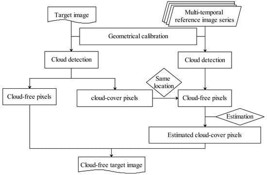
To generate a cloud-free image with clouds removed using the proposed approach, we need to perform geometric registration between the target image and the reference images and identify whether the pixel is cloud-free or cloudy. The procedure contains three parts (Figure 1): geometric calibration for registration of the reference images to the target one so that their pixels are kept the spatial consistency, cloud detection to identify the cloud cover pixels in both target and reference images, and estimation of the DN values for the cloud cover pixels of the target image using the multi-temporal reference images as assistance.
2.2. Geometric Correction
Since cloud removal is done in the target image with the assistance of reference ones, the prerequisite is to register the target and reference images into the same geographical positioning, which can be done through so-called geometric correction. In this study we used Landsat8 OLI images as an example to demonstrate the cloud removal, and we adopted a precise geometric correction with very high accuracy of geometric matching to be within one pixel of the same pixels in the target and the reference images. To ensure this accuracy, geometric calibration has been carefully performed on the OLI images used in the study using ERDAS IMAGINE from ERDAS Inc. in USA.
2.3. Cloud Detection
Foga et al. [35] compared the performances of many available cloud detection algorithms in the literature and assessed the accuracy of multiple cloud masking algorithms. The Fmask (Function of mask) algorithm has relatively better accuracy than the other algorithms from their validation tests across different parts of the world [12,35]. Qiu et al. [13] built the MFmask (Mountainous Fmask) algorithm upon the basis of the Fmask algorithm [12,20], which aims to detect clouds and cloud shadows in mountainous areas, where the Fmask algorithm does not perform well. Additionally, the MFmask algorithm can also work well for relatively flat terrain.
In the study we used the MFmask algorithm to achieve automated cloud and cloud shadow detection for Landsat8 OLI images. To improve the performance of the proposed linear regression modeling (LRM) algorithm and decrease the influence of the undetected contaminated pixels close to the edge, we performed a five-pixel buffer to the cloud and cloud shadow detection results with the cloudy pixels set to 0 and the cloud-free ones assigned as 1.
2.4. DN Value Estimation for the Cloud Cover Pixels
As seen in Equation (1), if the DN value of cloud covered pixel q (denoted as DNq,k for band k) in the target image is directly replaced by the DN value of the corresponding cloud-free pixel p in the reference image, it would lead to the spectral and radiometric in-comparability and inconsistency between the replaced pixel and the original one. To ensure this spectral and radiometric comparability and consistency, the SD in Equation (1) for the cloudy pixel should be estimated using the spectral similarity between the target and reference images. This can be done by considering the spectral difference between several cloud-free pixels spatially neighboring the cloud cover pixels between the target image and the reference one and then establishing the spectral similarity between target image and the reference one to estimate the DN value for the cloudy pixel. Figure 3 illustrates this procedure used in the study. Therefore, when we go over the pixels in the target image and find one with cloud covered, we turn to the reference image 1 (having the closest imaging date to the target image) to check its cloud detection result to confirm that it is clear or cloudy. If it is cloudy, then continue to the next reference image, i.e., reference image 2 (having the second closest image interval to the target one) and so on, until we find a cloud-free pixel in the reference image for the same geographic location of the cloud cover pixel in the target image. With this searching process, we can determine the reference images used to reconstruct the correspoding cloudy pixels in the target image. The next step is to establish the spectral similarity between the target and reference images.
When the corresponding cloud-free pixel p in the reference image is found, then search 10 cloud-free pixels around the pixel p (defined as surrounding pixels) in both the target and reference images using a sub-window searching technique. To quantitatively define the spectral comparability and consistency in cloud removing procedure, we computed the spectral difference between these surrounding pixels from the pixel p in the reference image for the band k, as follows:
where SDi,k is the spectral difference of the surrounding cloud-free pixel i from the pixel p in the reference image for the band k, DNi,k and DNp,k are the DN values of the pixel i and the pixel p for the band k, respectively.
SDi,k = |DNi,k − DNp,k|
From these surrounding pixels, we find out 10 ones having the least spectral differences from the pixel p, i.e., having the smallest SDi given from the above formula, defined as seed pixels:
where RIk denotes as data series of the seed pixels for band k, RI1,k, RI2,k, RI3,k, RI4,k, … and RI10,k are the spectral reflectance (DN values) of the seed pixels 1, 2, 3, 4, … and 10 for band k, respectively. Similarly, the corresponding pixels of these seed pixels in the target image are defined as the correlated pixels, as follows:
where TIk denotes data series of the seed pixels for band k, TI1,k, TI2,k, TI3,k, TI4,k, … and TI10,k are respectively the spectral reflectance (DN values) of the seed pixels 1, 2, 3, 4, … and 10 for band k in the target image. Using these two data series i.e., TIk and RIk, with TIk as dependent variable and RIk as independent variable, we can establish their linear regression equation, as follows:
where YTI,k is the dependent variable corresponding to the DN value for band k in the target image, XRI,k is the independent variable corresponding to the DN value for band k in the reference image, a and b are the regression coefficients of the equation. Using this equation, we can estimate the DN value for the cloudy pixel q in the target image from the corresponding cloud-free pixel p in the reference image for band k, as follows:
where DNq,k is the estimated DN value for the cloud cover pixel q for band k in the target image and DNp,k is the real DN value of the corresponding cloud-free pixel p for band k in the reference image. Since the above approach estimates the DN values for cloudy pixels through linear regression modeling (LRM), we term it as the LRM approach for cloud removal in the VNIR bands.
RIk = (RI1,k, RI2,k, RI3,k, RI4,k, RI5,k, RI6,k, RI7,k, RI8,k, RI9,k, RI10,k)
TIk = (TI1,k, TI2,k, TI3,k, TI4,k, TI5,k, TI6,k, TI7,k, TI8,k, TI9,k, TI10,k)
YTI,k = a + b XRI,k
DNq,k = a + b DNp,k
2.5. Validation of the Approach
To validate the proposed LRM approach, we used the Landsat5 TM images around Nanjing, Jiangsu Province (Figure 2) in Southeast China as experiments to perform the cloud removal procedures. Yangtze River, the biggest river in China, runs through the images from the south to the north. It can be said that the region covered by the image represents an economically developed area with dense population in East China. There are four major cities in the region: Nanjing, Ma’anshan, Wuhu and Chaohu. A large lake named Shijiu Lake is located at the lower right part of the image. Several low mountains are also observed in the image: Xihua Mountain, Zijin Mountain, Rufang Mountain and Jiangjun Mountain. Surface patterns in the region are complicated, representative and heterogeneous, including city, water, plain and mountain, which are required to validate the approach for cloud removal. Four Landsat5 TM images (p120r38) acquired, respectively, on DOY (Day-Of-Year) 140 (19 May), 124 (3 May), 108 (17 April) and 60 (29 February) in 2000 were used. We defined the image acquired on DOY 140 as the target image and the other three are the reference images.
For the validation of the approach, we need to compare the results of cloud removal, i.e., comparing the estimated DN values of the cloudy pixels by the approach with their true DN values to determine the accuracy of cloud removal by the approach. The contaminated images cannot be directly used for the validation because the true DN values of the contaminated pixels are unknown. To meet this requirement of validation, cloud-free images were used with a patch assumed to be cloud-contaminated in the target image. Using the assumed cloud area, we can know the true DN values of the assumed cloudy pixels and conduct the above cloud removal process to estimate the DN values for the assumed cloudy pixels. Comparing the estimated DN values for the assumed cloudy pixels with their true or original DN values over the target image, we can evaluate the accuracy of the proposed approach using the root mean square error (RMSE), and the value is defined as follows:
where Yi are the original DN values of the cloudy pixels and Yi’ is the estimated DN values of the corresponding cloudy pixels, N denotes the number of pixels used in validation. RMSE represents the absolute accuracy of the estimated DN values from their true ones in general for the cloudy pixels. We also used the relative estimation accuracy W, which is defined as follows:
where W is the relative estimation accuracy, M is the mean of the DN values of the patch for the experiment of validation. We can expect that the accuracy of the estimation is higher if the value of W is relatively higher.
Since the ground surface of the Earth is diverse, complicated and heterogeneous, the validation of the proposed approach is to be done with consideration of surface pattern, size of the contaminated patch and the imaging date of the reference images. For the surface pattern, we mainly considered four representative patterns in the region for the validation, such as plain, water, mountain and city areas. For the size of contaminated patch, we consider six patches assumed to be contaminated with 5 × 5, 10 × 10, 20 × 20, 50 × 50, 75 × 75 and 100 × 100 pixels, respectively, corresponding to small, middle and large cloudy areas. Considering the irregular condition, we performed the reconstruction procedure in low mountain area with an assumed irregular cloudy patch. For imaging date, we used three reference images acquired on DOY 124 (3 May), 108 (17 April) and 60 (29 February) in 2000, representing different intervals to the imaging date of the target image acquired on DOY 140 (19 May) in 2000.
To demonstrate the applicability of the proposed approach, we compared it with the available two conventional methods for cloud removal: directional replacement (DR) method and mean and standard deviation (MSD) transformation method presented by Surya and Simon [23]. Considering brightness difference between the target and reference images, Surya and Simon [23] performed brightness correction in their estimation of cloudy pixels’ values for the target image using the following equation:
where DNq,k is the estimated DN value for the cloud cover pixel q for band k in the target image, and DNp,k is the DN value of the corresponding cloud-free pixel p for band k in the reference image. MIT and MIR are denoted as the mean values of the target and reference image, respectively. DIT and DIR refer to the standard deviation values of the target and reference images.
The DR method represents the conventional reconstruction of missing information of the ground surface as a result of cloud cover from multi-temporal images. Due to spectral change during the interval of two images, the DR method usually leads to the sharp spectral difference between the original pixels and the reconstructed ones in the result image. In order to overcome this sharp difference, several approaches have been developed and the linear transformation combining the mean and standard deviation of the target and reference images to estimate the DN values for the contaminated pixels of the target image represents the best method for cloud removal in VNIR bands. As demonstrated in their study [23], this method can successfully reduce the spectral heterogeneity after reconstruction of missing information in the contaminated pixels due to its consideration of the spectral change between the target and reference images for the reconstruction.
2.6. Image Processing Procedure of the Approach
The satellite images for cloud removal can be defined as T(t), in which t refers to the acquired date of the images. For the convenience, we assigned the target image for cloud removal as T(0), and the reference images as T(−1), T(−2), … and T(j), in which T(−1) and T(−2) represent the reference image respectively having the closest and the 2nd closest acquired date to that of the target image T(0), and so on. Since we want to estimate the DN values for the cloudy pixel in all the VNIR bands of the target image, we denote the parameter k as the band number of the images. Thus, we have T(0,i,k), T(−1,i,k), T(−2,i,k) … and T(j,i,k), respectively, representing the ith pixel of the band k in target image T(0) and reference image T(−1), T(−2), and so on. The above approach for cloud removal to estimate DN values of the cloud cover pixels can be summarized as the following steps (Figure 3):
- (1)
- Perform geometric correction of the images T(0), T(−1), T(−2), … and T(j) to make sure that their corresponding pixels are spatially in the same geometric position, respectively.
- (2)
- Perform cloud detection to all the images T(0), T(−1), T(−2), … and T(j) to result in their corresponding cloud-mask images C(0), C(−1), C(−2), … and C(j) in which all the pixels are classified as cloud-free pixels with the values set to 1 and cloud-cover pixels set to 0.
- (3)
- Find a cloudy pixel in the target image. This can be done as the procedures: read the ith pixel of the cloud-mask image C(0,i) to determine if the ith pixel in the target image T(0) is cloud-free or cloud-cover. If C(0,i) = 1, the pixel is clear. Then we proceed to read the next pixel (i + 1) of the cloud-mask image C(0,i + 1) and determine if it is clear or cloudy. We continue this procedure until we find a cloud cover pixel C(0,i).
- (4)
- Find the corresponding cloud-free pixel of C(0,i) in the reference images. This can be done as follows: For j = −1, read C(−1,i) to determine if it is clear or not. If C(−1,i) = 0, it is cloudy and we go to next reference image (j = j − 1) to see if the corresponding pixel C(j,i) is cloudy or not until we obtain a cloud-free pixel C(j,i) that equals to 1.
- (5)
- Find 10 neighboring cloud-free pixels centering the cloud cover pixel C(0,i) in the target image T(0) and its corresponding cloud-free pixel C(j,i) in the reference image T(j). This can be done as follows: set 2 searching windows with sufficient sizes such as 5 × 5, 7 × 7, 9 × 9, …, 301 × 301, … pixels centering respectively C(0,i) and C(j,i) and the maximum window is set to m. Computing the spectral difference SDi,k between the pixel C(j,i) and its 10 neighboring pixels in the band k using the Equation (2) to determine their spectral similarity in the band k and set a threshold value n such as 5, 10, 15, 20, 30, 40, 50 … 100, etc. Enlarge the size of the window until we can get 10 corresponding cloud-free pixels that the SDi,k is less than n in two windows, if still not at the maximum window then gradually enlarge threshold value from 5, 10, 15, …, 50, …, 100, … and continue to search ranging from the minimum window size until you find the 10 available pixels.
- (6)
- Establish the dataset TIk of the target image and the RIk of the reference image for the band k. Using the 10 pixels from the step (5), we go to the reference image T(j) to obtain their pixel values to establish dataset RIk. Using the corresponding location of these 10 pixels in the target image, we can also easily get the dataset TIk.
- (7)
- Establish spectral regression between the two datasets TIk and RIk. We can obtain Equation (5) through the least square method of regression analysis with the pixel values in TIk as the dependent variable and those in RIk as the independent variable.
- (8)
- Estimate the DN value of the cloud cover pixel in the target image. We can get DNq,k in Equation (6) using the DN value corresponding to the cloud-free pixel C(i,j) = 1 in reference image T(j) and Equation (6) for band k.
- (9)
- Estimate the DN values of the cloud cover pixel in the target image for other bands. Continue the above steps (5)–(8) until all the bands have been completed.
- (10)
- Repeat the above steps (3)–(9) until all the cloudy pixels in the target image have been removed with their DN values estimated for all the bands.
3. Result and Analysis
3.1. Accuracy of Cloud Removal over Various Ground Surface Patterns
Mountain, plain, water and city represent the four representative patterns of land surface found in the real world. Table 1 shows the accuracy of cloud removal over these surface patterns for a small patch (10 × 10 pixels) assumed to be cloud covered in the TM image (p120r38) acquired on DOY 140 (19 May) in 2000 as the target image in Nanjing of East China. As shown in Table 1, the LRM approach is generally better with the lowest RMSEs among the three methods used to validate the accuracy of cloud removal in the TM image, implying its highest accuracy for cloud removal among the three methods. Table 1 indicates that, for water-covered area near Nanjing, the LRM approach has RMSE of 1.25 for cloud removal in band 1, while it is 7.61 and 2.28 for the DR and MSD method when the image acquired on DOY 124 (3 May) in 2000 was used as reference image. The lowest RMSEs of our LRM approach were also seen for band 2 and 4, respectively (Table 1). For band 3, we have even lower RMSE 0.91 than that for band 1. The RMSE of the LRM approach is 0.68 for band 4 in the near infrared band, which is also the lowest among the three methods.
Comparison of our LRM approach with the other two methods was also done for the plain and city surface patterns, which have more complicated surface structure, hence, they were usually categorized as the heterogeneous surface patterns with great spectral difference in the spatial dimension. As seen in Table 1, even though the LRM approach still has the lowest RMSEs among the three methods for the two heterogeneous surfaces for all bands of the TM images, the relatively higher RMSEs were observed for the two surface patterns than those for mountain and water surfaces. For example, for band 2 we have RMSE of 0.99 for the LRM approach applying to the mountain area, while it was 1.25 for the plain surface and 1.12 for the city surface (Table 1).
RMSE represents the average error of estimation. If we divide it by the mean value of the patch, we would get the relative accuracy of the estimation. When all the values are accurately estimated, the RMSE would be the minimum so that the parameter W would be maximum of 1. Table 1 shows that our LRM approach generally has W values of 98% for the water pattern, which is slightly higher than the MSD method, implying that our proposed LRM approach can improve the estimation accuracy of DN values for the cloudy pixels. For the mountain area, the W value is high, up to 98%, while it is only about 94–98% for the MSD method (Table 1). For LRM, the highest RMSE 3.07 is in the plain area (band 4) and lowest W (0.96) is located in the plain area (band 3 and band 4), we can still find that LRM is more accurate. In Table 1, relatively better performance of our proposed LRM approach can be found for all the four surface patterns, which confirms its applicability as an alternative for cloud removal in the VNIR regions of spectrum for remote sensing image process. The scatter plots of the three methods for four bands over the mountain surface pattern are shown in Figure 4.
3.2. Impact of Reference Images on Accuracy of Cloud Removal
Due to the seasonal change, we can expect that the spectral change and underlying surface change may be obvious as imaging interval increases, which consequently has important impact on the accuracy of cloud removal. In order to reveal this impact, we compare the RMSEs of our LRM approach with the other two conventional methods using three images acquired on DOY 124 (3 May), 108 (17 April) and 60 (29 February) in 2000, respectively, for cloud removal over two representative surface patterns (city and water). Table 2 shows the results of this comparison over a small patch (20 × 20 pixels) assumed to be cloud covered. The image acquired on DOY 124 has the smallest imaging interval from the target image (acquired on DOY 140) among the three reference images. We can see that the RMSEs of DOY 124 are the smallest in comparison with the other two reference images of DOY 108 and 60 among the three methods in the city area (Table 2). The DR method has a RMSE of 8.14 for band 1 for the city surface when the image of DOY 124 was used as the reference, while this RMSE would reach up to 33.34 for the same band and the same city surface when the image of DOY 60 was used as the reference image. With respect to the LRM approach, the image of DOY 124 only has an RMSE of 2.31 for band 1, which is smaller than the RMSE of the MSD method. We can also see that the RMSE of our LRM approach in band 3 increases from 1.62 for the DOY 124 image to 2.95 for the DOY 60 image. The RMSEs become greater as the imaging interval of the reference image increases from that of the target images in the city area.
While there is no similar impact observed over the water surface that the RMSEs are increased with the acquisition intervals (Table 2). This is mainly attributed to the impact of spectral difference and underlying surface change between the target image and the reference one in the water area is less than those in the city area. As can be seen in Table 2, this sharp change of spectral difference consequently shapes remarkable impact of the accuracy of the cloud removal. Despite this increase in RMSE with the imaging interval between the reference and the target images, it can still be observed that our approach has the lowest RMSEs for all the three bands among the three methods. Moreover, the RMSEs of the MSD method are also very small and its W values are also very high, indicating that this method is also very good in cloud removal to generate cloud-free image.
For intuitively comparing the impact of the imaging interval between the target and reference image on cloud removal through the three methods, cloud removal validation test was performed in a 100 × 100 pixel patch within Nanjing City. The performance of the reconstructed results by the three methods is consistent with the quality index statistics. As the DR method results show in Figure 5d–f, when the imaging interval between the target image and the reference one increases, the DN value difference between them is enlarged and the DR result using the reference image captured on DOY 60 shows the worst radiometric consistency. The same impact is observed in the cloud removal results of the MSD and LRM methods. However, comparing the reconstructed results (Figure 5f,i,l) of the three methods using the reference image captured on DOY 60 (29 February) in 2000, the LRM result (Figure 5l) shows more consistency and fewer effects by the sharp change of spectral difference between the target image captured on DOY 140 (19 May) and the reference image captured on DOY 60. The same condition can be seen from the reconstructed results using the reference image captured on DOY 124 (3 May) and 108 (17 April) in Figure 6. Thus, the acquisition time of the reference images would not seriously affect the reconstruction performance of the proposed LRM method compared with the other two methods.
3.3. Effect of Cloud Cover Sizes on Accuracy of Cloud Removal
Clouds and cloud shadows in the sky always have different sizes and shapes. The above validation was done to the medium size of cloudy patch with 10 × 10 and 20 × 20 pixels. In order to reveal the impact of cloud cover magnitude on the accuracy of our LRM approach in cloud removal, we assumed six sizes with 5 × 5, 10 × 10, 20 × 20, 50 × 50, 75 × 75 and 100 × 100 pixels of cloudy patches to compare the LRM approach with the two other methods in the mountainous area using the reference image acquired on DOY 124.
The reconstruction accuracy of different sizes of cloud-cover patches in the mountainous area as shown in Table 3. The proposed LRM approach generally has the lowest RMSEs but the highest W values among the three methods for the different sizes of patches assumed to be cloudy. Thus, the LRM method in the validation test of TM image shows the highest accuracy among the three methods on cloud removal. For the minimum 5 × 5 pixels of the cloud cover patch, the LRM approach has the lowest RMSE of 0.80 for cloud removal in band 2 of the TM image, while it is high, up to 4.04, and 1.30 for the DR and MSD methods when the image captured on DOY 124 was used as the reference image. The lowest RMSE of the LRM approach was also seen for band 4, the RMSE of the LRM approach is 2.23 for band 4 the near infrared regions of the spectrum (Table 3). And comparison of the LRM approach with the other two methods was also done for the assumed cloudy patch (100 × 100 pixels) in the mountain area.
As seen in Table 3, the LRM approach still has the lowest RMSEs among the three methods for the other five larger size patches for all the bands of the TM images, the relatively higher RMSEs were observed for the other two methods. Additionally, there is no apparent tendency for the reconstructed results that the RMSEs increase with patch enlarging, implying that the patch size enlargement would not always increase the RMSEs or cause relatively lower accuracy.
Figure 6 shows the reconstructed images with a patch assumed to be cloudy containing 100 × 100 pixels by the three methods using the reference image acquired on DOY 124. In accordance with the quality index characteristic, the LRM reconstructed image (Figure 6d) has lowest RMSEs in all the four bands (respectively, 1.57, 0.91, 1.13 and 3.16 for bands 1, 2, 3 and 4). It shows better radiometric consistency with the surrounding cloud-free pixels than the results by the DR method (Figure 6b) and MSD method (Figure 6c). Clouds usually appear in irregular shapes instead of rectangles or squares. Thus, we also need to examine the effect of cloud shape on the accuracy of the pixels’ DN value estimation for cloud removal using the proposed approach. We designed an irregular cloud patch and compared our approach with the other two methods. As we can see from Figure 6, the reconstructed result (Figure 6h) by our proposed LRM shows a better radiometric consistency than the DR result (Figure 6f) and MSD result (Figure 6g), which also has a more similar structure with the target image in Figure 6e. Therefore, the LRM algorithm is also applicable for the irregular size of cloud removal.
3.4. Application to Southeast China Region
We applied the procedures of the proposed LRM approach to Southeast China using Landsat8 OLI imagery. As shown in Figure 7, the image acquired on 29 April 2016 in the Nanjing area was viewed as the target image, and two images acquired on 28 March and 12 March 2016 were used as reference ones. Considering the influences of the cloud shapes and different land surface patterns, we selected five subset areas containing 1000 × 1000 pixels to test the proposed LRM method for bands 4, 3, 2 (RGB) and band 5 (NIR). The five subset areas cover representative land cover patterns, such as plain, city, water and mountain. The relatively large-scale clouds and scattered clouds with obvious cloud shadows were all processed in the application of the LRM method using OLI images.
As seen from Figure 8a,b, the cloud and cloud shadow detection results in the lower left show that the shapes of the extracted clouds and shadows are relatively complete and natural compared with the original image and the cloud shadow edge can be relatively fully extracted. In Figure 8, the reconstructed area that is covered by the clouds and cloud shadows contains water, mountain and city. The reconstructed result in lower right shows a relatively coherent visual effect on brightness in the cloud removal result, implying its comparability and radiometric consistency with the target image.
Considering the relatively larger-scale clouds and cloud shadows that often appear, site C and D in Figure 7a were chosen as application tests. As shown in Figure 9a (site C), a series of stripped clouds and their shadows cover over the Yangtaze River area containing various land surface patterns, while in Figure 9b (site D) clouds, along with their shadows, are distributed between the Nanyi River in the south and Gucheng River in the North of Xuanzhou City. The reconstructed pixels by the LRM method for cloud and cloud shadow removal in the lower right panel show good consistency with the neighboring original pixels. Thus, the proposed LRM method can also be used in the relatively large-scale thick cloud removal.
We also compared the LRM reconstructed result of RGB bands (bands 4, 3 and 2) and the NIR band (band 5) in Figure 10 for the site E in Figure 7a. The cloud removal image in Figure 10a (bands 4, 3 and 2, composited) and Figure 10b (bands 5, 4 and 3 composited) both show good radiometric consistency, indicating high accuracy in DN value estimation by the LRM method for all four bands including NIR band 5.
4. Discussion
The simulated experiments indicate that the proposed LRM reconstruction algorithm is reliable for all the underlying surfaces tested. All the reconstructed areas are highly consistent with the original areas. The actual experiments also illustrate the consistency between the reconstructed DN values and the surrounding cloud-free DN values. Therefore, the proposed LRM method can reconstruct cloud-contaminated pixels accurately under different land cover types.
The new LRM method also shows some advantages compared with the existing approaches. The cloud removal results from the proposed LRM method have less edge effects, which implies feasibility for the case of heterogeneous underlying surfaces and various sizes of cloud and cloud shadows. In addition, usage of auxiliary images with relatively long interval, such as several days, has no significant influence to the cloud removal result, which reduces the limitation of temporally close auxiliary reference images unavailability, especially in the tropical areas. Compared to the other two methods, the proposed method was evaluated under a range of land cover types, showing lowest RMSEs and lowest W values at different sites. This suggests that the proposed LRM method is quite effective and stable in most cases.
Additionally, it should be addressed that the proposed method is limited for the images with very large-scale thick clouds covered and without enough information of neighboring cloud-free pixels. The future line of research is to improve the proposed method by developing the nonlinear method [36] and dealing with the large-scale cloud reconstruction.
5. Conclusions
An efficient approach is proposed in this study to remove thick clouds along with their shadows. The basic idea is to reconstruct the cloud cover pixels of the target image with the DN values estimated with the LRM method using several close cloud-free pixels centered the cloudy pixels of both target and multi-temporal reference images for each VNIR band. A series of procedures have been developed for the cloud removal including geometric correction, cloud detection and estimation of the DN values. With this technique, the reconstructed pixels are comparable with those cloud-free ones of the image.
To demonstrate the advantage of the approach, we compared it with two available methods for cloud removal: the DR and MSD methods. Four TM images around Nanjing city of Jiangsu Province in Eastern China were used to validate the approach over four representative surface patterns (mountain, plain, water and city) for seven various sizes of cloud covered. The LRM method has better reconstruction accuracy (lowest RMSEs) and comparable visual quality for the VNIR bands of the images. We also performed the LRM approach to Southeast China using Landsat8 OLI image for bands 4, 3, 2 (RGB) and band 5 (NIR) with the two previous images as reference ones. Five subset areas of a size of 1000 × 1000 pixels were used to test the LRM method over different sizes of cloud cover and various representative underlying surface patterns. Very good radiometric consistency is observed in the cloud removal results.
The proposed LRM method for cloud removal keeps the original DN values of cloud-free pixels in the target image and only the DN values of the cloudy pixels are reconstructed with a pixel by pixel and band to band process using reference images. The results show good spectral comparability and radiometric consistency with the target image. We confirm that the proposed approach could serve as an alternative for cloud removal along with their shadows in the VNIR bands using multi-temporal remote sensing images, which is useful for many remote sensing and GIS applications that require more cloud-free images, such as land cover, change detection, time series analyses and NDVI value estimation.
Author Contributions
Data curation, W.D.; Funding acquisition, Z.Q.; Methodology, W.D., Z.Q., J.F. and F.W.; Software, W.D., J.F., F.W. and B.A.; Supervision, Z.Q., J.F. and M.G. Validation, W.D.; Writing—original draft, W.D.; Writing—review & editing, W.D., Z.Q., J.F., M.G. and B.A.
Funding
This study was supported by the General Project of National Natural Science Foundation of China (Grant No. 41471300, 41771406) and the Collaborative Innovation Project of CAAS Innovation Program (Grant No. CAAS-XTCX2016007-4).
Acknowledgments
We sincerely thanks Aruhan Bao, Huanran Yue, Ye Li, Chenguang Wang and Qianyu Liao from Chinese Academy of Agricultural Sciences for their assistance in image preprocessing and statistics for the study.
Conflicts of Interest
The authors declare no conflict of interest. The funders had no role in the design of the study; in the collection, analyses, or interpretation of data; in the writing of the manuscript, or in the decision to publish the results.
References
- Duan, S.B.; Li, Z.L.; Tang, B.H.; Wu, H.; Tang, R.L. Generation of a time-consistent land surface temperature product from MODIS data. Remote Sens. Environ. 2014, 140, 339–349. [Google Scholar] [CrossRef]
- Liang, L.; Zhao, S.H.; Qin, Z.H.; He, K.X.; Chong, C.; Luo, Y.X.; Zhou, X.D. Drought change trend using MODIS TVDI and its relationship with climate factors in china from 2001 to 2010. J. Integr. Agric. 2014, 13, 1501–1508. [Google Scholar] [CrossRef]
- Li, Z.L.; Becker, F. Feasibility of land surface temperature and emissivity determination from AVHRR data. Remote Sens. Environ. 1993, 43, 67–85. [Google Scholar] [CrossRef]
- Duan, S.B.; Li, Z.L.; Leng, P. A framework for the retrieval of all-weather land surface temperature at a high spatial resolution from polar-orbiting thermal infrared and passive microwave data. Remote Sens. Environ. 2017, 195, 107–117. [Google Scholar] [CrossRef]
- Rozenstein, O.; Qin, Z.; Derimian, Y.; Karnieli, A. Derivation of land surface temperature for landsat-8 tirs using a split window algorithm. Sensors 2014, 14, 5768–5780. [Google Scholar] [CrossRef]
- Ren, H.; Ye, X.; Liu, R.; Dong, J.; Qin, Q. Improving land surface temperature and emissivity retrieval from the Chinese gaofen-5 satellite using a hybrid algorithm. IEEE Trans. Geosci. Remote Sens. 2017, 56, 1080–1090. [Google Scholar] [CrossRef]
- Gao, M.F.; Qin, Z.H.; Zhang, H.O.; Lu, L.P.; Zhou, X.; Yang, X.C. Remote sensing of agro-droughts in Guangdong province of China using MODIS satellite data. Sensors 2008, 8, 4687–4708. [Google Scholar] [CrossRef] [PubMed]
- Leng, P.; Song, X.N.; Duan, S.B.; Li, Z.L. A practical algorithm for estimating surface soil moisture using combined optical and thermal infrared data. Int. J. Appl. Earth. Obs. 2016, 52, 338–348. [Google Scholar] [CrossRef]
- Tang, R.L.; Li, Z.L.; Tang, B.H. An application of the Ts-VI triangle method with enhanced edges determination for evapotranspiration estimation from MODIS data in arid and semi-arid regions: Implementation and validation. Remote Sens. Environ. 2010, 114, 540–551. [Google Scholar] [CrossRef]
- Tang, B.H.; Li, Z.L.; Zhang, R.H. A direct method for estimating net surface shortwave radiation from MODIS data. Remote Sens. Environ. 2006, 103, 115–126. [Google Scholar] [CrossRef]
- Goodwin, N.R.; Collett, L.J.; Denham, R.J.; Flood, N.; Tindall, D. Cloud and cloud shadow screening across Queensland, Australia: An automated method for Landsat TM/ETM+ time series. Remote Sens. Environ. 2013, 134, 50–65. [Google Scholar] [CrossRef]
- Zhu, Z.; Woodcock, C.E. Object-based cloud and cloud shadow detection in Landsat imagery. Remote Sens. Environ. 2012, 118, 83–94. [Google Scholar] [CrossRef]
- Qiu, S.; He, B.; Zhu, Z.; Liao, Z.; Quan, X. Improving Fmask cloud and cloud shadow detection in mountainous area for Landsats 4-8 images. Remote Sens. Environ. 2017, 199, 107–119. [Google Scholar] [CrossRef]
- Xu, M.; Jia, X.P.; Pickering, M.; Plaza, A.J. Cloud removal based on sparse representation via multitemporal dictionary learning. IEEE Trans. Geosci. Remote Sens. 2016, 54, 2998–3006. [Google Scholar] [CrossRef]
- Chang, N.B.; Bai, K.; Chen, C.F. Smart information reconstruction via time-space-spectrum continuum for cloud removal in satellite images. IEEE J. STARS 2015, 8, 1898–1912. [Google Scholar] [CrossRef]
- Hagolle, O.; Huc, M.; Pascual, D.V.; Dedieu, G. A multi-temporal method for cloud detection, applied to FORMOSAT-2, VENμS, LANDSAT and SENTINEL-2 images. Remote Sens. Environ. 2010, 114, 1747–1755. [Google Scholar] [CrossRef]
- Jin, S.; Homer, C.; Yang, L.; Xian, G.; Fry, J.; Danielson, P.; Townsend, P.A. Automated cloud and shadow detection and filling using two-date Landsat imagery in the USA. Int. J. Remote Sens. 2013, 34, 1540–1560. [Google Scholar] [CrossRef]
- Roy, D.P.; Ju, J.; Kline, K.; Scaramuzza, P.L.; Kovalskyy, V.; Hansen, M.; Loveland, T.R.; Vermote, E.; Zhang, C.S. Web-enabled Landsat data (weld): Landsat ETM+ composited mosaics of the conterminous United States. Remote Sens. Environ. 2010, 114, 35–49. [Google Scholar] [CrossRef]
- Wilson, M.J.; Oreopoulos, L. Enhancing a simple MODIS cloud mask algorithm for the Landsat data continuity mission. IEEE Trans. Geosci. Remote Sens. 2013, 51, 723–731. [Google Scholar] [CrossRef]
- Zhu, Z.; Wang, S.; Woodcock, C.E. Improvement and expansion of the fmask algorithm: Cloud, cloud shadow, and snow detection for Landsats 4-7, 8, and sentinel 2 images. Remote Sens. Environ. 2015, 159, 269–277. [Google Scholar] [CrossRef]
- Shen, H.F.; Li, X.H.; Cheng, Q.; Zeng, C.; Yang, G.; Li, H.F.; Zhang, L.P. Missing information reconstruction of remote sensing data: A technical review. IEEE Geosci. Remote Sens. Mag. 2015, 3, 61–85. [Google Scholar] [CrossRef]
- Shen, H.F.; Li, H.F.; Qian, Y.; Zhang, L.P.; Yuan, Q.Q. An effective thin cloud removal procedure for visible remote sensing images. ISPRS J. Photogramm. 2014, 96, 224–235. [Google Scholar] [CrossRef]
- Surya, S.R.; Simon, P. Automatic cloud removal from multitemporal satellite images. J. Indian Soc. Remote 2014, 43, 57–68. [Google Scholar] [CrossRef]
- Chen, B.; Huang, B.; Chen, L.F.; Xu, B. Spatially and temporally weighted regression: A novel method to produce continuous cloud-free Landsat imagery. IEEE Trans. Geosci. Remote Sens. 2016, 55, 27–37. [Google Scholar] [CrossRef]
- Maalouf, A.; Carre, P.; Augereau, B.; Maloigne, C.F. A bandelet-based inpainting technique for clouds removal from remotely sensed images. IEEE Trans. Geosci. Remote Sens. 2009, 47, 2363–2371. [Google Scholar] [CrossRef]
- Zhu, X.; Gao, F.; Liu, D.; Chen, J. A modified neighborhood similar pixel interpolator approach for removing thick clouds in Landsat images. IEEE Geosci. Sens. Lett. 2012, 9, 521–525. [Google Scholar] [CrossRef]
- Melgani, F. Contextual reconstruction of cloud-contaminated multitemporal multispectral images. IEEE Trans. Geosci. Remote Sens. 2006, 44, 442–455. [Google Scholar] [CrossRef]
- Eckardt, R.; Berger, C.; Thiel, C.; Schmullius, C. Removal of optically thick clouds from multi-spectral satellite images using multi-frequency SAR data. Remote Sens. 2013, 5, 2973–3006. [Google Scholar] [CrossRef]
- Huang, B.; Li, Y.; Han, X.Y.; Cui, Y.Z.; Li, W.B.; Li, R.R. Cloud removal from optical satellite imagery with SAR imagery using sparse representation. IEEE Geosci. Remote Sens. Lett. 2017, 12, 1046–1050. [Google Scholar] [CrossRef]
- Xu, M.; Pickering, M.; Plaza, A.J.; Jia, X.P. Thin cloud removal based on signal transmission principles and spectral mixture analysis. IEEE Trans. Geosci. Remote Sens. 2016, 54, 1659–1669. [Google Scholar] [CrossRef]
- Li, X.H.; Shen, H.F.; Zhang, L.P.; Zhang, H.Y.; Yuan, Q.Q.; Yang, G. Recovering quantitative remote sensing products contaminated by thick clouds and shadows using multitemporal dictionary learning. IEEE Trans. Geosci. Remote Sens. 2014, 52, 7086–7098. [Google Scholar]
- Lin, C.H.; Tsai, P.H.; Lai, K.H.; Chen, J.Y. Cloud removal from multitemporal satellite images using information cloning. IEEE Trans. Geosci. Remote Sens. 2013, 51, 232–241. [Google Scholar] [CrossRef]
- Valero, S.; Pelletier, C.; Bertolino, M. Patch-based reconstruction of high resolution satellite image time series with missing values using spatial, spectral and temporal similarities. In Proceedings of the 2016 IEEE International Geoscience and Remote Sensing Symposium (IGARSS), Beijing, China, 10–15 July 2016; pp. 2308–2311. [Google Scholar]
- Cheng, Q.; Shen, H.F.; Zhang, L.P.; Yuan, Q.Q.; Zeng, C. Cloud removal for remotely sensed images by similar pixel replacement guided with a spatio-temporal MRF model. ISPRS J. Photogramm. 2014, 92, 54–68. [Google Scholar] [CrossRef]
- Foga, S.; Scaramuzza, P.L.; Guo, S.; Zhu, Z.; Jr, R.D.D.; Beckmann, T.; Schmidt, G.L.; Dwyer, J.L.; Hughes, M.J.; Laue, B. Cloud detection algorithm comparison and validation for operational Landsat data products. Remote Sens. Environ. 2017, 194, 379–390. [Google Scholar] [CrossRef] [Green Version]
- Safont, G.; Salazar, A.; Vergara, L.; Rodríguez, A. Nonlinear estimators from ICA mixture models. Signal Process. 2019, 155, 281–286. [Google Scholar] [CrossRef]
Figure 1.
Framework illustrating the approach for cloud removal using multi-temporal reference images.
Figure 1.
Framework illustrating the approach for cloud removal using multi-temporal reference images.

Figure 2.
Landsat5 TM images used for validation of the approach, with (a) showing the geographical location of the image in East China, (b) TM image of Nanjing region in the Low Reach Basin of the Yangtze River, the largest river in China. The ground surfaces of mountain (c), plain (d) water (e) and city (f) area used for the experiments to validate the approach.

Figure 3.
Schematic diagram of the cloud removal approach.

Figure 4.
The scatter plots of the 3 methods for the 4 bands over the mountain surface patterns with (a–c) for band 1; (d–f) for band 2; (g–i) for band 3; (j–l) for band 4.
Figure 4.
The scatter plots of the 3 methods for the 4 bands over the mountain surface patterns with (a–c) for band 1; (d–f) for band 2; (g–i) for band 3; (j–l) for band 4.

Figure 5.
Reconstruction of the target TM image (p120r38) captured on DOY 140 using the three approaches with the reference image captured on DOY 124 for the 100 × 100 pixel patch (inside black line) in urban area (bands 1, 4 and 3 composited as RGB). (a–c) represent the reference images captured on DOY 124, 108 and 60 in the city area, respectively. (d–f) show the reconstructed images by the DR method using the reference image captured on DOY 124, 108 and 60, respectively. (g–i) are the reconstructed results by MSD method using the reference images captured on DOY 124, 108 and 60. (j–l) represent the reconstructed images by the LRM method using the reference images captured on DOY 124, 108 and 60. Cloud cover masks were made with cloudy pixels (inside the black line) set to 0 and cloud-free pixels (outside the black line) set to 1.

Figure 6.
Reconstruction of the target TM image captured on DOY 140 using the three approaches with the reference image captured on DOY 124 in the mountain area (bands 1, 4 and 3 composited). (a) The target image captured on DOY 140 in the mountain area with 100 × 100 pixels (inside the black line). (b–d) The reconstructed images by DR, MSD and LRM methods using the reference image captured on DOY 124 for 100 × 100 pixel (inside the black line) cloudy patch. (e) The irregular size cloudy patch (inside the black line) of the target image captured on DOY 140 over the mountain area. (f–h) The reconstructed images by DR, MSD and LRM methods using the reference image captured on DOY 124 for the irregular size cloud. Cloud masks with cloudy pixels (inside black line) set to 0 and cloud-free pixels (outside the black line) assigned as 1.

Figure 7.
Applying the LRM approach to the OLI image located in Southeast China near Nanjing City. (a) The target image captured on 29 April 2016 with five subset test areas (bands 4, 3 and 2 composited) containing different land cover patterns. (b,c) The reference images acquired on 28 March and 12 March 2016 were used to reconstruct the cloudy areas.

Figure 8.
LRM results of small scattered patch from Landsat8 OLI image (p120r38_20160429) located in Southeast China near Nanjing City (1000 × 1000 pixel subset). (a,b) are two tests about removal of scattered clouds along with apparent cloud shadows shown in Figure 7a for site A and B (bands 5, 4 and 3 composited). Upper left shows a subset of Landsat8 OLI image with cloud and cloud shadow covered. Upper right represents the corresponding subset of the reference OLI image (p120r38_20160328). Lower right is the corresponding reconstructed result by the proposed LRM algorithm. Lower left refers to the corresponding MFmask results, including clouds (white), cloud shadows (red) and clear sky (black).

Figure 9.
LRM results of a small scattered patch of clouds from Landsat8 OLI image(p120r38_20160429) located in Southeast China near Nanjing City (1000 × 1000 pixel subset). The (a,b) are two tests with a relatively larger-scale clouds and cloud shadows shown in Figure 7a of site C and D (composited bands 5, 4 and 3). Upper left shows a subset of Landsat8 OLI image with cloud and cloud shadow cover. Upper right represents the corresponding subset of the reference OLI image (p120r38_20160328). Lower right is the corresponding reconstructed results by the proposed LRM algorithm. Lower left represents the corresponding MFmask results, containing clouds (white), cloud shadows (red) and clear sky (black).

Figure 10.
LRM results from Landsat8 OLI image (p120r38_20160429) for site E in Figure 7a located in Southeast China near Nanjing City (1000 × 1000 pixel subset), (a) (bands 4, 3 and 2 composited) and (b) (bands 5, 4 and 3 composited). Upper left shows a subset of Landsat8 OLI images with cloud and cloud shadow cover. Upper right shows the corresponding subset of the reference OLI image (p120r38_20160328). Lower right shows the corresponding reconstructed results by the proposed LRM algorithm. (a) (bands 4, 3 and 2 composited), Lower left represents the MFmask results containing clouds (white), cloud shadows (red) and clear sky (black). (b) (bands 5, 4 and 3 composited), lower left shows the corresponding subset of the reference OLI image (p120r38_20160312).


Table 1.
Accuracy of cloud removal for a small patch (10 × 10 pixels) assumed cloud cover over representative surface patterns in the TM image of Nanjing.
Table 1.
Accuracy of cloud removal for a small patch (10 × 10 pixels) assumed cloud cover over representative surface patterns in the TM image of Nanjing.
| Surface Patterns | Methods | RMSE | W | ||||||
|---|---|---|---|---|---|---|---|---|---|
| Band1 | Band2 | Band3 | Band4 | Band1 | Band2 | Band3 | Band4 | ||
| Water | DR | 7.61 | 4.70 | 3.77 | 6.47 | 0.93 | 0.91 | 0.93 | 0.81 |
| MSD | 2.28 | 1.09 | 1.58 | 3.46 | 0.98 | 0.98 | 0.97 | 0.90 | |
| LRM | 1.25 | 0.86 | 0.91 | 0.68 | 0.99 | 0.98 | 0.98 | 0.98 | |
| Plain | DR | 7.54 | 4.97 | 8.36 | 7.41 | 0.93 | 0.90 | 0.86 | 0.91 |
| MSD | 2.01 | 1.34 | 2.49 | 3.24 | 0.98 | 0.97 | 0.96 | 0.96 | |
| LRM | 1.87 | 1.25 | 2.38 | 3.07 | 0.98 | 0.98 | 0.96 | 0.96 | |
| Mountain | DR | 8.98 | 4.33 | 6.58 | 5.73 | 0.90 | 0.89 | 0.83 | 0.94 |
| MSD | 1.90 | 1.31 | 2.50 | 5.53 | 0.98 | 0.97 | 0.94 | 0.94 | |
| LRM | 1.69 | 0.99 | 0.98 | 1.92 | 0.98 | 0.98 | 0.97 | 0.98 | |
| City | DR | 7.60 | 5.44 | 7.03 | 6.64 | 0.93 | 0.90 | 0.88 | 0.89 |
| MSD | 1.97 | 1.22 | 1.80 | 1.89 | 0.98 | 0.98 | 0.97 | 0.97 | |
| LRM | 1.92 | 1.12 | 1.74 | 1.73 | 0.98 | 0.98 | 0.97 | 0.97 | |
Note: In the table DR represents the direct replacement method, MSD is the mean and standard deviation method and LRM is the proposed method. RMSE is denoted in Equation (7); W is defined in Equation (8), which represents the relative accuracy of the corresponding method used for cloud removal in the experiment.
Table 2.
Accuracy of cloud removal over a small patch (20 × 20 pixels) assumed to be cloudy using three different reference images in the TM image of Nanjing.
Table 2.
Accuracy of cloud removal over a small patch (20 × 20 pixels) assumed to be cloudy using three different reference images in the TM image of Nanjing.
| Surface Patterns | DOY | Methods | RMSE | W | ||||||
|---|---|---|---|---|---|---|---|---|---|---|
| Band1 | Band2 | Band3 | Band4 | Band1 | Band2 | Band3 | Band4 | |||
| City | DOY124 | DR | 8.14 | 5.56 | 7.22 | 7.02 | 0.93 | 0.90 | 0.88 | 0.89 |
| MSD | 2.37 | 1.32 | 1.86 | 1.82 | 0.98 | 0.98 | 0.97 | 0.97 | ||
| LRM | 2.31 | 1.29 | 1.62 | 1.78 | 0.98 | 0.98 | 0.97 | 0.97 | ||
| DOY108 | DR | 19.50 | 11.01 | 13.61 | 13.58 | 0.83 | 0.79 | 0.78 | 0.78 | |
| MSD | 2.90 | 1.84 | 2.38 | 2.90 | 0.97 | 0.97 | 0.96 | 0.95 | ||
| LRM | 2.02 | 1.36 | 1.75 | 2.42 | 0.98 | 0.97 | 0.97 | 0.96 | ||
| DOY60 | DR | 33.34 | 19.19 | 24.25 | 29.75 | 0.71 | 0.64 | 0.60 | 0.52 | |
| MSD | 5.20 | 3.00 | 5.82 | 5.48 | 0.95 | 0.94 | 0.90 | 0.91 | ||
| LRM | 2.97 | 1.90 | 2.95 | 3.84 | 0.97 | 0.96 | 0.95 | 0.94 | ||
| Water | DOY124 | DR | 7.39 | 4.43 | 3.75 | 6.74 | 0.94 | 0.92 | 0.94 | 0.89 |
| MSD | 2.24 | 1.28 | 1.67 | 3.07 | 0.98 | 0.98 | 0.97 | 0.95 | ||
| LRM | 1.41 | 1.02 | 0.93 | 0.87 | 0.99 | 0.98 | 0.98 | 0.99 | ||
| DOY108 | DR | 17.19 | 8.39 | 8.92 | 10.98 | 0.85 | 0.84 | 0.85 | 0.82 | |
| MSD | 2.52 | 1.86 | 1.86 | 6.96 | 0.98 | 0.97 | 0.97 | 0.89 | ||
| LRM | 1.57 | 0.95 | 0.97 | 0.95 | 0.99 | 0.97 | 0.98 | 0.92 | ||
| DOY60 | DR | 24.14 | 14.59 | 16.61 | 11.74 | 0.79 | 0.73 | 0.73 | 0.81 | |
| MSD | 3.53 | 2.43 | 2.79 | 8.57 | 0.97 | 0.95 | 0.95 | 0.86 | ||
| LRM | 1.42 | 1.02 | 1.01 | 0.96 | 0.99 | 0.98 | 0.98 | 0.97 | ||
Table 3.
Accuracy of cloud removal over six sizes of patches assumed to be cloudy using the reference image captured on DOY 124 for the TM image in the mountainous area of Nanjing.
Table 3.
Accuracy of cloud removal over six sizes of patches assumed to be cloudy using the reference image captured on DOY 124 for the TM image in the mountainous area of Nanjing.
| Quality Index | Band | 5PIX-DOY124 | 10PIX-DOY124 | 20PIX-DOY124 | ||||||
|---|---|---|---|---|---|---|---|---|---|---|
| DR | MSD | LRM | DR | MSD | LRM | DR | MSD | LRM | ||
| RMSE | Band1 | 8.56 | 1.55 | 1.48 | 8.98 | 1.90 | 1.69 | 9.55 | 1.87 | 1.67 |
| Band2 | 4.04 | 1.30 | 0.80 | 4.33 | 1.31 | 0.99 | 4.90 | 1.25 | 1.01 | |
| Band3 | 6.40 | 1.96 | 1.00 | 6.58 | 2.50 | 0.98 | 7.29 | 2.13 | 1.22 | |
| Band4 | 4.61 | 5.23 | 2.23 | 5.73 | 5.53 | 1.92 | 6.87 | 5.79 | 3.26 | |
| W | Band1 | 0.91 | 0.98 | 0.98 | 0.90 | 0.98 | 0.98 | 0.90 | 0.98 | 0.98 |
| Band2 | 0.90 | 0.97 | 0.98 | 0.89 | 0.97 | 0.98 | 0.88 | 0.97 | 0.97 | |
| Band3 | 0.84 | 0.95 | 0.97 | 0.83 | 0.94 | 0.97 | 0.81 | 0.95 | 0.97 | |
| Band4 | 0.95 | 0.95 | 0.98 | 0.94 | 0.94 | 0.98 | 0.93 | 0.94 | 0.96 | |
| Quality Index | Band | 50PIX-DOY124 | 75PIX-DOY124 | 100PIX-DOY124 | ||||||
| DR | MSD | LRM | DR | MSD | LRM | DR | MSD | LRM | ||
| RMSE | Band1 | 9.33 | 1.81 | 1.69 | 9.28 | 1.85 | 1.59 | 9.20 | 2.00 | 1.57 |
| Band2 | 4.76 | 1.31 | 0.98 | 4.87 | 1.32 | 0.93 | 4.89 | 1.42 | 0.91 | |
| Band3 | 7.25 | 2.01 | 1.42 | 7.28 | 2.10 | 1.20 | 7.32 | 2.41 | 1.13 | |
| Band4 | 6.24 | 6.01 | 3.02 | 6.02 | 6.65 | 3.17 | 6.19 | 6.92 | 3.16 | |
| W | Band1 | 0.90 | 0.98 | 0.98 | 0.90 | 0.98 | 0.98 | 0.90 | 0.98 | 0.98 |
| Band2 | 0.88 | 0.97 | 0.98 | 0.88 | 0.97 | 0.98 | 0.88 | 0.97 | 0.98 | |
| Band3 | 0.81 | 0.95 | 0.96 | 0.81 | 0.95 | 0.97 | 0.82 | 0.94 | 0.97 | |
| Band4 | 0.94 | 0.94 | 0.97 | 0.94 | 0.93 | 0.97 | 0.94 | 0.93 | 0.97 | |
© 2019 by the authors. Licensee MDPI, Basel, Switzerland. This article is an open access article distributed under the terms and conditions of the Creative Commons Attribution (CC BY) license (http://creativecommons.org/licenses/by/4.0/).
Share and Cite
MDPI and ACS Style
Du, W.; Qin, Z.; Fan, J.; Gao, M.; Wang, F.; Abbasi, B. An Efficient Approach to Remove Thick Cloud in VNIR Bands of Multi-Temporal Remote Sensing Images. Remote Sens. 2019, 11, 1284. https://doi.org/10.3390/rs11111284
AMA Style
Du W, Qin Z, Fan J, Gao M, Wang F, Abbasi B. An Efficient Approach to Remove Thick Cloud in VNIR Bands of Multi-Temporal Remote Sensing Images. Remote Sensing. 2019; 11(11):1284. https://doi.org/10.3390/rs11111284
Chicago/Turabian StyleDu, Wenhui, Zhihao Qin, Jinlong Fan, Maofang Gao, Fei Wang, and Bilawal Abbasi. 2019. "An Efficient Approach to Remove Thick Cloud in VNIR Bands of Multi-Temporal Remote Sensing Images" Remote Sensing 11, no. 11: 1284. https://doi.org/10.3390/rs11111284
Note that from the first issue of 2016, this journal uses article numbers instead of page numbers. See further details here.