Improved Modeling of Gross Primary Productivity of Alpine Grasslands on the Tibetan Plateau Using the Biome-BGC Model


1
Key Laboratory of Digital Earth Science, Institute of Remote Sensing and Digital Earth, Chinese Academy of Sciences, Beijing 100094, China
2
College of Resources and Environment, University of Chinese Academy of Sciences, Beijing 100049, China
3
Key Laboratory of Land Surface Pattern and Simulation, Institute of Geographical Sciences and Natural Resources Research, Chinese Academy of Sciences, Beijing 100101, China
*
Author to whom correspondence should be addressed.
Remote Sens. 2019, 11(11), 1287; https://doi.org/10.3390/rs11111287
Submission received: 15 April 2019
/
Revised: 27 May 2019
/
Accepted: 28 May 2019
/
Published: 30 May 2019
(This article belongs to the Special Issue Terrestrial Carbon Cycle)
Abstract
:The ability of process-based biogeochemical models in estimating the gross primary productivity (GPP) of alpine vegetation is largely hampered by the poor representation of phenology and insufficient calibration of model parameters. The development of remote sensing technology and the eddy covariance (EC) technique has made it possible to overcome this dilemma. In this study, we have incorporated remotely sensed phenology into the Biome-BGC model and calibrated its parameters to improve the modeling of GPP of alpine grasslands on the Tibetan Plateau (TP). Specifically, we first used the remotely sensed phenology to modify the original meteorological-based phenology module in the Biome-BGC to better prescribe the phenological states within the model. Then, based on the GPP derived from EC measurements, we combined the global sensitivity analysis method and the simulated annealing optimization algorithm to effectively calibrate the ecophysiological parameters of the Biome-BGC model. Finally, we simulated the GPP of alpine grasslands on the TP from 1982 to 2015 based on the Biome-BGC model after a phenology module modification and parameter calibration. The results indicate that the improved Biome-BGC model effectively overcomes the limitations of the original Biome-BGC model and is able to reproduce the seasonal dynamics and magnitude of GPP in alpine grasslands. Meanwhile, the simulated results also reveal that the GPP of alpine grasslands on the TP has increased significantly from 1982 to 2015 and shows a large spatial heterogeneity, with a mean of 289.8 gC/m2/yr or 305.8 TgC/yr. Our study demonstrates that the incorporation of remotely sensed phenology into the Biome-BGC model and the use of EC measurements to calibrate model parameters can effectively overcome the limitations of its application in alpine grassland ecosystems, which is important for detecting trends in vegetation productivity. This approach could also be upscaled to regional and global scales.
1. Introduction
Gross Primary Productivity (GPP), defined as the total amount of carbon fixed by vegetation through photosynthesis, is one of the most important components of the terrestrial carbon cycle [1,2]. Meanwhile, it is also the largest carbon flux between the terrestrial biosphere and the atmosphere, and drives a variety of ecosystem services such as food, fiber, and wood production [3]. The Tibetan Plateau (TP), with an average elevation exceeding 4000 m, is one of the most sensitive regions to global climate change [4]. Moreover, due to the positive feedbacks associated with the melting of snow and ice, the warming rate on the TP is expected to be much higher than other regions over China [5,6]. Such a unique geographical environment makes the circulation of carbon on the TP different from other regions. Therefore, accurate estimation of GPP on the TP and continuous monitoring of its spatial and temporal dynamics are needed to enhance our understanding of terrestrial ecosystems and global carbon cycling.
As of now, many models have been developed to estimate GPP at the regional scale, which can be divided into statistical models [7], light use efficiency models [8,9], and process-based models [10,11,12]. Based on these models, numerous studies have quantified GPP of alpine grasslands on the TP [13,14,15,16]. However, it should be mentioned that there are large differences between the GPP values estimated by different studies, which greatly impeded our understanding of the feedback mechanisms between the terrestrial ecosystems and the atmosphere. For example, Zhuang et al. [13] estimated annual GPP of alpine grasslands on the TP as 712 gC/m2/yr by the Terrestrial Ecosystem Model (TEM), which is 2.28 times the estimate of He et al. [14], in which annual GPP of alpine grasslands was quantified at 312.3 gC/m2/yr by the Vegetation Photosynthesis Model (VPM). The large model uncertainty may be attributed to the inadequate calibration of model parameters, especially for complex process-based models. Therefore, it is necessary to develop an effective parameter calibration method capable of adapting the model to particular applications.
The Biome-BGC model is a typical process-based biogeochemical model that can be used to simulate the carbon, nitrogen, and water fluxes within terrestrial ecosystems [11]. Initially, the application of the Biome-BGC model was mainly focused on forest ecosystems [17,18,19]. Recently, some studies have applied this model to grassland ecosystems [20,21]. However, in addition to the aforementioned difficulties of parameter calibration in the process-based model, the phenology module of the Biome-BGC also has limitations, especially when applied to alpine regions. Specifically, this phenology module assumes that leaf onset occurs when both the summed soil temperature and the summed precipitation are greater than the critical values, and leaf senescence occurs when the date has passed July 1st and the average minimum temperature for the next 3 days is less than the annual average minimum temperature [22]. Nevertheless, for alpine regions like the TP, frozen soil, glaciers, and snow are usually widely distributed, and their seasonal thawing can provide water for the germination and growth of alpine vegetation, which in turn will affect phenological shifts [23]. Unfortunately, the original phenology module in the Biome-BGC has not taken into account the effects of frozen soil and snow, which caused a significant delay in the simulated leaf onset date and further led to a severe underestimation of GPP [21]. Therefore, it is necessary to modify the phenology module of the Biome-BGC to make it applicable to alpine regions.
In recent years, the development of remote sensing technology has made it possible to extract phenological parameters on the regional scale. Due to its advantages such as wide coverage, spatial continuity, and long time series, many studies have used remote sensing-derived vegetation index to extract phenological metrics on the TP [24,25,26]. However, to the best of our knowledge, no research has been conducted on combining remotely sensed phenology with the Biome-BGC model to improve its simulation performance in alpine regions, although many studies have shown that combining higher precision phenological data with process-based models can improve the performance of carbon flux simulation [27,28,29].
To this end, we first used the remotely sensed phenology to prescribe the phenological states within the Biome-BGC model. Then, we used the global sensitivity analysis method to identify those ecophysiological parameters that have a significant impact on the GPP simulation. Subsequently, we performed a calibration upon these specific parameters using the simulated annealing optimization algorithm in conjunction with the eddy covariance (EC)-derived GPP data. Finally, we used the Biome-BGC model after a phenology module modification and parameter calibration to simulate the GPP of alpine grasslands on the TP from 1982 to 2015. Our objectives were threefold: (1) to investigate whether the integration of remotely sensed phenology and the Biome-BGC model can improve the performance of carbon flux simulation of alpine grasslands on the TP; (2) to develop a practical parameter calibration method for complex process-based models; (3) to analyze the spatial and temporal variation of GPP of alpine grasslands on the TP from 1982 to 2015.
2. Study Area and Dataset
2.1. Study Area
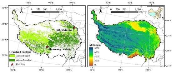
The TP, located in the southwest of China, is the largest and highest plateau in the world. It covers an area of approximately km2 and has an average elevation of more than 4000 m [30]. At the same time, it is also known as “the Third Pole of the Earth” and “the Roof of the World”. Due to its high altitude and complex geographic environment, the TP has formed a unique climate condition characterized by low air temperature, long sunshine duration, and strong solar radiation [31]. Such a special climate environment also promotes the formation of a typical alpine vegetation ecosystem. The dominant vegetation type on the TP is alpine grassland, with an area of about km2, including alpine steppe and alpine meadow (Figure 1) [32]. At the same time, the TP is rich in frozen soil, snow, and glacial resources, and their melting water makes the TP the source of several major rivers such as the Yellow River and the Yangtze River. On the other hand, the TP is also extremely sensitive to global climate change. It has been reported that the mean annual temperature on the TP has increased by 0.3 °C per decade over the past 50 years, much higher than other regions of China [5]. Such a sharp warming trend has had a great impact on the alpine vegetation ecosystem, such as advanced spring phenology and enhanced plant carbon fixation [6,23,25].
2.2. Dataset
2.2.1. Meteorological Forcing and Land Surface Initial Conditions for the Biome-BGC Model
In order to estimate the GPP of alpine grasslands at the regional scale, the Biome-BGC model needs spatially explicit forcing data and a vegetation distribution map. The forcing data used to run the Biome-BGC model includes daily meteorological data, land surface initialization data, and ecophysiological parameters. Among them, ecophysiological parameters need to be carefully calibrated to adapt the model to particular applications. For alpine meadows and alpine steppes, both of them are classified as C3 grass in the Biome-BGC model and contains a total of 28 ecophysiological parameters (Table 1). In this study, we used the EC-derived GPP to calibrate these ecophysiological parameters and evaluate the simulation performance of the Biome-BGC model. A detailed description of these data is as follows. In addition, all of the following spatially explicit data was resampled to resolution.
(1) Daily meteorological data used to drive the Biome-BGC model mainly includes precipitation, temperature, shortwave radiation, day length, and vapor pressure deficit (VPD). They were calculated from the China Meteorological Forcing Dataset (http://westdc.westgis.ac.cn) using the MT-CLIM tool. Among them, the China Meteorological Forcing Dataset has a 0.1° spatial resolution and a daily temporal resolution, spanning the period from 1982 to 2015, and the MT-CLIM tool is a program released with the Biome-BGC that can be used to estimate missing daily meteorological data that is not available from in situ measurements [33]. In this study, we used the MT-CLIM tool to estimate the day length and VPD that were not included in the China Meteorological Forcing Dataset.
(2) Land surface initialization data mainly contains soil texture (percentage of sand, clay, and silt), soil depth, elevation, shortwave albedo, atmospheric CO2 concentration, and atmospheric nitrogen deposition. Among them, soil texture and soil depth were obtained from Soil Map Based Harmonized World Soil Database (v1.2) provided by Cold and Arid Regions Sciences Data Center with a spatial resolution of 30 arc-second. Elevation data was acquired from STRM 90m Digital Elevation Database provided by CGIAR Consortium for Spatial Information (available at http://www.cgiar-csi.org). Shortwave albedo data with a spatial resolution of was obtained from the National Earth System Science Data Sharing Infrastructure, National Science & Technology Infrastructure of China (available at http://www.geodata.cn). Atmospheric CO2 concentration data was obtained from the National Oceanic and Atmospheric Administration (NOAA) (available at ftp://ftp.cmdl.noaa.gov/ccg/co2/trends/). Atmospheric nitrogen deposition data at a resolution was supplied by the Chinese Academy of Agricultural Sciences.
(3) The EC flux data at two flux sites was obtained from the Chinese Flux Observation and Research Network (ChinaFLUX), which was used to calibrate the ecophysiological parameters corresponding to alpine meadows and alpine steppes, respectively. A detailed description of these two flux sites are given in Table 2, and information on the EC measurement system can be found in [34]. The initial measured fluxes (Net Ecosystem Exchange, NEE) were first processed by the ChinaFLUX CO2 data processing system [35]. Then, the linear interpolation model and the Michaelis–Menten equation were used to fill small gaps (less than 2 h) and large gaps in the time series, respectively [36]. Subsequently, daytime ecosystem respiration was calculated using the Lloyd and Taylor method combined with nighttime observations [37]. Finally, GPP was estimated as the difference between daytime NEE and ecosystem respiration.
(4) The distribution map of alpine grassland was derived from the digitized 1:1 million vegetation map of the TP compiled by Institute of Geographic Sciences and Natural Resources Research, Chinese Academy of Sciences (Figure 1).
2.2.2. GIMMS NDVI Dataset and Preprocessing
Normalized difference vegetation index (NDVI), defined as the difference between the near-infrared and red reflections divided by the sum of the two, is a dimensionless index that can be used to estimate the density of green on an area of land [40]. The Global Inventory Modeling and Mapping Studies (GIMMS) NDVI3g.v1 dataset, with a spatial resolution of and a temporal resolution of 15-day intervals, has been the most widely used remote sensing product for monitoring vegetation phenology over large areas [41]. It was generated from the Advanced Very High Resolution Radiometer (AVHRR) sensors onboard on several NOAA satellites. At the same time, it was also the latest version of the GIMMS NDVI dataset, spanning the period from January 1982 to December 2015. This dataset has improved data quality at high latitudes, especially in regions where the growing season is shorter than 2 months [42].
Before using the GIMMS NDVI dataset, some preprocessing procedures were needed to reduce the effects of clouds and the atmosphere. Specifically, the maximum value composition (MVC) was first applied to the NDVI dataset to eliminate noises caused by cloud and snow contamination [43]. Then, the Savitzky–Golay filter was used to remove outliers and smooth the NDVI time series [44]. Finally, regions with a multiyear average NDVI less than 0.1 were excluded from the analysis to further minimize the impacts of barren land and non-vegetation [24].
3. Methodology
The methodology of this study is composed of four key steps. Firstly, the original phenology module of the Biome-BGC was modified by remotely sensed phenology, which was achieved by using the phenological indicators derived from remote sensing to prescribe the phenological states within the Biome-BGC model. Secondly, based on the Biome-BGC model after a phenology module modification, the Morris qualitative sensitivity analysis method was used to screen out those parameters that have negligible effects on the GPP simulation, and then the Sobol’ quantitative sensitivity analysis method was used to evaluate the influence of each of the remaining parameters on the simulated GPP and further determine the parameters to be calibrated. Moreover, considering the differences in the physiological characteristics of alpine meadows and alpine steppes, we performed a sensitivity analysis on them separately. Thirdly, we used the simulated annealing optimization algorithm combined with EC-derived GPP data to calibrate those influential parameters selected in the previous step, and set those non-influential parameters to the default values. This calibration process was also performed on alpine meadows and alpine steppes, respectively. In addition, since only two years of EC-derived GPP data was obtained for both alpine meadows and alpine steppes, we used the first year of GPP data to calibrate the influential parameters while using the second year of GPP data to validate the performance of the Biome-BGC model. Finally, we extrapolated the Biome-BGC model after a phenology module modification and parameter calibration to the entire alpine grasslands on the TP to simulate its GPP from 1982 to 2015. Figure 2 shows the organizational flow chart of the methodology of this study, and details will be given in the subsequent sections.
3.1. The Biome-BGC Model
Biome-BGC is a process-based biogeochemical model used to simulate the carbon, nitrogen, and water cycles within the terrestrial ecosystems from a single plot to regional and global scales [11]. It uses a daily time-step and was developed from the Forest-BGC model [45]. Previous studies have successfully applied this model to a variety of biomes such as forests and grasslands [17,18,20,46]. There are several critical processes in the Biome-BGC model, including photosynthesis, respiration, evapotranspiration, decomposition, the allocation of photosynthetic assimilates, and mortality [11]. To model the photosynthesis process, the Biome-BGC model converts leaf C into an equivalent leaf area by multiplying the user-defined specific leaf area (SLA) parameters. SLA is a measure of the thickness of a leaf and is defined as the leaf area per unit mass. The Biome-BGC model further partitions leaf C and leaf area into sunlit and shaded fractions using a two-leaf photosynthesis model [47,48] and calculates each photosynthetic process separately. The carbon flux simulated by the Biome-BGC model mainly includes GPP, Net Primary Productivity (NPP), Net Ecosystem Productivity (NEP), and NEE. Among them, GPP is the total carbon fixed by photosynthesis, NPP is the difference between GPP and autotrophic respiration, NEP is the difference between NPP and heterotrophic respiration, and NEE is the difference between NEP and the carbon loss caused by fire. In this study, we used the newly released Biome-BGC v4.2 to simulate the GPP of alpine grasslands on the TP (available at http://www.ntsg.umt.edu/project/biome-bgc.php).
3.2. Phenology Module Modification
Vegetation phenology determines the start (SOS) and end (EOS) of the growing season. Accurate representation of phenology is critical for terrestrial biosphere models to simulate the temporal dynamics of biological processes on the land surface [49]. The phenology module used in the Biome-BGC was developed based on the empirical relationship between phenology and meteorological conditions. It defines SOS as the date when both the summed precipitation and the summed soil temperature are greater than the critical values, and defines EOS as the date after July 1st where the average minimum temperature for the next 3 days is less than the annual average minimum temperature [22]. However, this module was found to have significantly delayed the SOS of vegetation in alpine regions, resulting in a severe underestimation of GPP [21]. To this end, we proposed to incorporate remotely sensed phenology into the Biome-BGC model to better prescribe the phenological states within the model. Specifically, we first extracted the SOS and EOS of alpine grasslands on the TP from 1982 to 2015 based on the GIMMS NDVI dataset, and then we used the SOS and EOS extracted from the NDVI dataset to prescribe the phenological states of vegetation within the Biome-BGC model. Through this modification, the Biome-BGC can effectively overcome the limitations of its original phenology module.
In order to extract phenological parameters from NDVI time series data, several methods have been proposed, such as the NDVI thresholds method [22,50], fitting logistic functions [51], largest NDVI increase method [52], and delayed moving average method [53]. Among them, the dynamic threshold method [50] has been proven to be one of the simplest and most effective methods for the extraction of phenological parameters [54,55]. Therefore, we also used this method to extract the SOS and EOS from the NDVI dataset. The ratio of NDVI is defined as
where represents the output ratio, ranging from 0 to 1, represents the daily NDVI, represents the annual maximum NDVI, and represents the annual minimum NDVI in the upward or downward direction, which corresponds to the calculation of SOS or EOS, respectively.
Based on the , the SOS and EOS are defined as the dates when the reaches the dynamic threshold of 0.2 in the upward and downward directions, respectively [55]. Accordingly, the length of growing season (LOS) can be defined as the difference between EOS and SOS.
3.3. Model Parameterization
Despite improvements in the phenology module of the Biome-BGC, additional model parameter calibration is still required to achieve accurate simulation of the GPP. However, the Biome-BGC model typically includes a large number of parameters, and these parameters are generally interdependent, making the calibration process very difficult. Therefore, prior to calibrating the model parameters, it is necessary to identify those parameters that have a significant impact on the simulated variables for further calibration. Global sensitivity analysis can quantify the contribution of uncertainty in model inputs to uncertainty in model outputs and allow for the evaluation of interactions between model inputs [56]. In this study, we also used the global sensitivity analysis to identify those ecophysiological parameters that have a significant impact on the GPP simulation. Then, we used the simulated annealing optimization algorithm in conjunction with EC-derived GPP data to calibrate those selected influential parameters to achieve model calibration.
In the Biome-BGC model, both alpine meadows and alpine steppes are classified as the type of C3 grass, which includes a total of 28 tunable ecophysiological parameters (Table 1). However, it should be noted that there are still some differences in the physiological characteristics between alpine meadows and alpine steppes. Therefore, in order to more accurately quantify the GPP of alpine grasslands on the TP, we performed a parameter sensitivity analysis and calibration on them separately. On the other hand, since only two years of EC-derived GPP data was obtained for each flux station, we used the first year of daily measured GPP to calibrate the influential parameters while using the second year of GPP data to validate its performance.
3.3.1. Sensitivity Analysis
Global sensitivity analysis typically requires a large amount of computational resources and is quite time-consuming. To overcome this limitation, we used a combination of qualitative sensitivity analysis and quantitative sensitivity analysis to identify those parameters that have a significant impact on the GPP simulation. Specifically, we first collected the probability distribution function (PDF) of the ecophysiological parameters of C3 grass from relevant literature, as shown in Table 1. Subsequently, we used the Morris qualitative analysis method [57] to screen out those ecophysiological parameters that have negligible effects on the GPP simulation and set them to the default values. Finally, we used the Sobol’ quantitative analysis method [58] to evaluate the influence of each of the remaining parameters on the GPP simulation and further determine which parameters to be calibrated. A detailed description of these steps is as follows.
• Distribution of ecophysiological parameters
In addition to the two phenological parameters for prescribing the phenological states within the model, the Biome-BGC includes a total of 28 tunable ecophysiological parameters for C3 grass. In addition, there is no evidence of periodic fires in alpine grasslands of the TP in the past few decades, so we set the fire mortality parameter to zero and did not calibrate it. Finally, a total of 27 parameters are left for the next sensitivity analysis, and their PDFs were collected from relevant literature, as shown in Table 1.
• Qualitative sensitivity analysis based on the Morris method
The Morris method is a typical One-at-a-Time sensitivity analysis method [57]. Due to its low computational cost, it is often used as the first step in global sensitivity analysis to remove parameters that have negligible effects on the simulated results. Two sensitivity indices, mean () and standard deviation (), are calculated by the Morris method to qualitatively evaluate the relative importance of each parameter. To perform the analysis, the Morris method needs to be executed times, where represents the number of trajectories and represents the number of input parameters. In this study, was set to 10 [56] and the value of was 27. In addition, we used the average of the annual GPP between 1982 and 2015 as the output variable of the Morris method and set a low threshold value of to distinguish between influential and non-influential parameters. That is, parameters with were considered to have negligible effects on the GPP simulation and were excluded from the next quantitative analysis. Further information on the Morris method can be found in the Supplementary Materials.
• Quantitative sensitivity analysis based on the Sobol’ method
The Sobol’ method is a widely used quantitative global sensitivity analysis method, which can decompose the variance of the model output into the contribution of each input parameter and their interactions [58]. Given that represents the total variance of the model output, it can be decomposed into the following components:
where represents the variance explained by the th input parameter, represents the variance explained by the interactions between the th and th input parameters, and represents the number of input parameters. Based on Equation (2), the first order sensitivity index can be defined as , and the higher order sensitivity indices can be defined as , ,, . Accordingly, the total order sensitivity index of the th parameter can be defined as the sum of its first order sensitivity index and all higher order sensitivity index involving it. In addition, a large difference between the first order sensitivity index and the total order sensitivity index indicates that the parameter mainly affects the model output through interactions.
The Sobol’ method uses the Monte Carlo [59] sampling scheme to generate random parameter samples. To calculate sensitivity metrics, it requires a parameter set with a sample size of , where represents the number of base samples and represents the number of input parameters. In this study, was set to 512. In addition, we used the total order sensitivity index to quantitatively evaluate the effect of each ecophysiological parameter on the GPP simulation and set its threshold to 0.05. That is, parameters with a total order sensitivity index greater than 0.05 were considered as influential parameters and required further calibration.
3.3.2. Parameter Calibration
The simulated annealing algorithm is a heuristic optimization algorithm based on Monte Carlo’s iterative solution [60]. It is able to find the optimal parameter values in the parameter space that enable the model to generate the best agreement between the simulation and the observation. In this study, we used this algorithm to calibrate the influential ecophysiological parameters selected by the Sobol’ method. Specifically, we first designed a cost function for the simulated annealing algorithm based on the difference between the observed GPP and the simulated GPP, with the following form:
where represents the sum of absolute errors, represents the daily GPP simulated by the Biome-BGC model, represents the daily GPP observed by the EC technique, and represents the number of observed values. Subsequently, we imported the PDFs of those influential ecophysiological parameters into the simulated annealing algorithm to generate new parameter values, and further calculated its corresponding cost function value. Then, we judged the cost function value according to the Metropolis criterion to decide whether to accept the new parameter values. Finally, the above two steps were repeated until the termination condition was reached. Through these iterative optimization processes, we have a high probability of obtaining global optimal parameter values.
3.4. Biome-BGC Model Simulation
The simulation of the Biome-BGC model consists of two phases, namely the spin-up simulation and the normal simulation. For the spin-up simulation phase, the Biome-BGC model started with constant preindustrial atmospheric CO2 concentration (286 ppm) and nitrogen deposition (0.0002 kgN/m2/yr) and looped through the meteorological data from 1982 to 2015 many times until a steady state was reached [61,62]. For the normal simulation phase, the results of the spin-up simulation were used as initial values for the carbon and nitrogen pools and then normal simulations were performed.
In this study, the original Biome-BGC model without any modifications was called Version-0 (V0), the Biome-BGC model whose phenology module was modified by remotely sensed phenology was called Version-1 (V1), and the Biome-BGC model after a phenology module modification and parameter calibration was called Version-2 (V2). In order to estimate the GPP of alpine grasslands at the regional scale, we first used the EC-derived GPP data to validate the performance of V2. Then, we extrapolated V2 to the entire alpine grasslands on the TP to simulate its GPP from 1982 to 2015.
4. Results and Analysis
4.1. Remotely Sensed Phenology
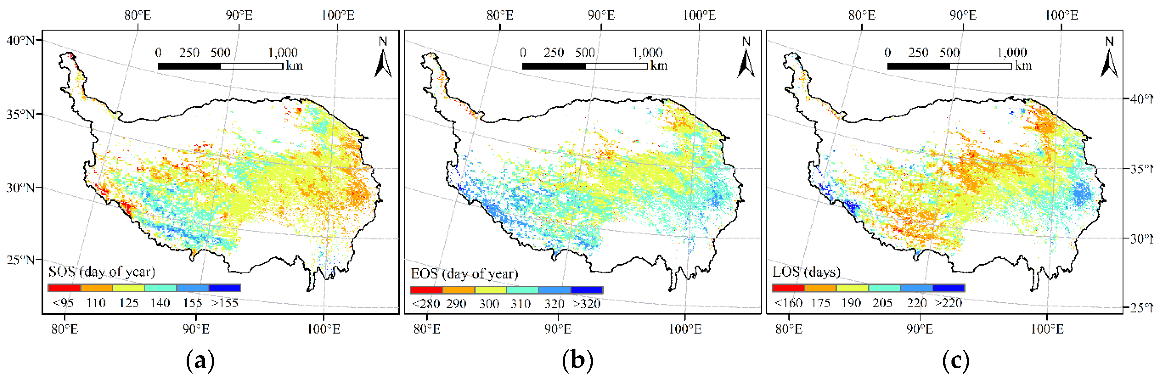
The spatial patterns of mean annual SOS, EOS, and LOS extracted from the NDVI time series data were provided in Figure 3. As depicted, the SOS showed a decreasing trend from west to east, consistent with the hydrothermal gradient of the TP. The EOS showed a large spatial heterogeneity across the TP and roughly exhibited a decreasing trend from south to north. Meanwhile, the LOS generally showed a decreasing trend from southeast to northwest, which is also consistent with the hydrothermal gradient on the TP. In addition, according to the statistical results, the SOS was mainly concentrated between the 100th and 150th days of the year, accounting for 95.4% of the alpine grassland area. The EOS mainly occurred between the 290th and 320th days of the year, accounting for 94.7% of the alpine grassland area. Furthermore, the LOS was mainly concentrated between 170 and 210 days, accounting for 85.3% of the alpine grassland area.
4.2. Parameter Sensitivity Analysis and Calibration
Based on the Biome-BGC model after a phenology module modification (V1), we used the Morris method and the Sobol’ method to identify those parameters that have a significant impact on the GPP simulation for further calibration. The results of Morris sensitivity analysis at Haibei Station and Damxung Station are shown in Figure S1. At Haibei Station, three ecophysiological parameters (Lcel, VPDi, and VPDf) had a Morris index () below the preset threshold of 0.05, and six ecophysiological parameters (Llig, FRcel, SLAsha:sun, Gbl, VPDi, and VPDf) at Damxung Station had a Morris index below the preset threshold. These parameters were considered to have negligible effects on the GPP simulation and were excluded from the next Sobol’ sensitivity analysis.
The results of Sobol’ sensitivity analysis of the remaining parameters at Haibei Station and Damxung Station are provided in Figure S2. As can be seen, at Haibei Station, the simulation of GPP was most sensitive to C:Nfr, and its large first order and total order sensitivity index values indicate that this parameter affects the GPP simulation either directly or through interaction. The second most influential parameters were C:Nleaf and C:Nlit. Among them, C:Nleaf mainly affects GPP through interaction, while C:Nlit directly controls the simulation of GPP. Interestingly, similar sensitivity analysis results also appeared in Damxung Station, which suggests that there is no significant difference between the parameters that have an important impact on the GPP simulation of alpine meadows and alpine steppes. To further determine the influential parameters to be calibrated, we set the threshold of the total order sensitivity index to 0.05. Through screening, Haibei Station retained seven ecophysiological parameters and Damxung Station retained eight ecophysiological parameters, as shown in Table 3.
Based on these selected influential parameters, we used the simulated annealing optimization algorithm combined with EC-derived GPP data to calibrate these parameters to achieve model parameterization. The calibrated results for Haibei Station and Damxung Station are provided in Table 3.
4.3. Site-Level Evaluation
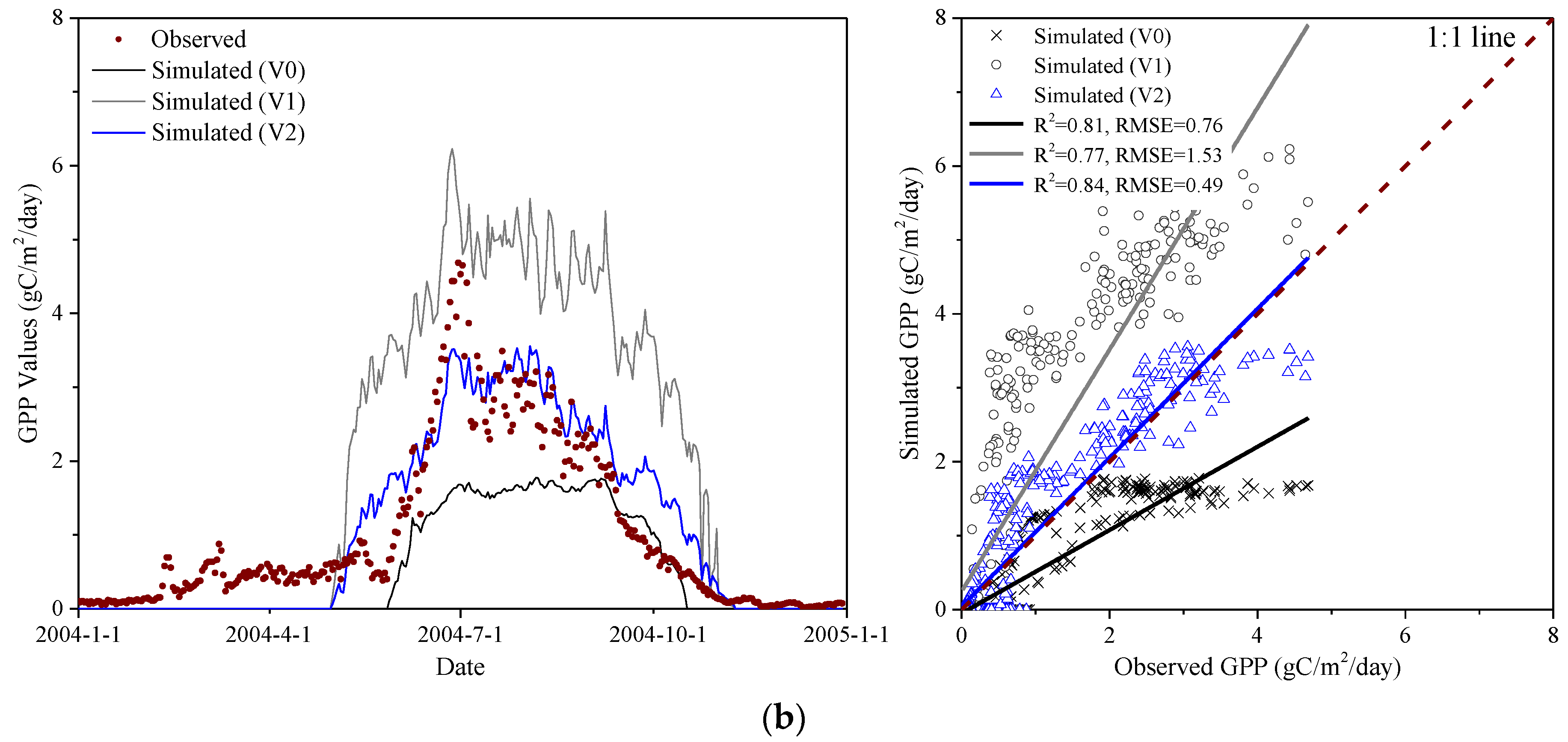
The effects of phenology on GPP simulation for the calibration year and the validation year are shown in Figure 4 and Figure S3, respectively. Among them, the calibration year represents the first year of the acquired EC-derived GPP data, which is used for model calibration, and the validation year represents the second year of the acquired EC-derived GPP data, which is used for model validation. As can be seen from Figure 4 and Figure S3, V0 severely underestimated the GPP values at both Haibei Station and Damxung Station as compared to the EC-derived GPP (marked with red dots). However, the GPP simulated by V1 effectively overcame this limitation, which indicated that remotely sensed phenology can more realistically reflect the phenological characteristics of alpine grasslands on the TP. The reason for the substantial underestimation of GPP in V0 is mainly attributable to the severe lag in the simulation of SOS, which directly leads to a shortened LOS and further affects the carbon fixation process of vegetation. Nevertheless, it should be noted that there was still a large difference between the GPP simulated by V1 and the GPP derived from EC measurements, so further calibration of V1 is still necessary.
A comparison of GPP simulations before and after calibration for the calibration year and the validation year were shown in Figure 4 and Figure S3, respectively. As depicted in Figure 4, V2 significantly improved the simulation accuracy of GPP and showed the best performance in all versions of the Biome-BGC model. Compared with the initial version V0, the RMSE of the final version V2 was reduced by 1.49 gC/m2/day at Haibei Station and 0.27 gC/m2/day at Damxung Station, and its coefficient of determination increased by 0.08 and 0.03 at Haibei Station and Damxung Station, respectively. However, it should be mentioned that the simulation accuracy of V2 is slightly lower than that of V0 at Damxung Station for the validation year (Figure S3), but it is still much higher than the simulation accuracy of V1. The reason may be attributable primarily to the relatively low carbon fixation rate at Damxung Station, while the GPP simulated by V0 is also underestimated due to the severe lag of the simulated SOS, thus making the GPP simulated by V0 close to the EC-derived GPP.
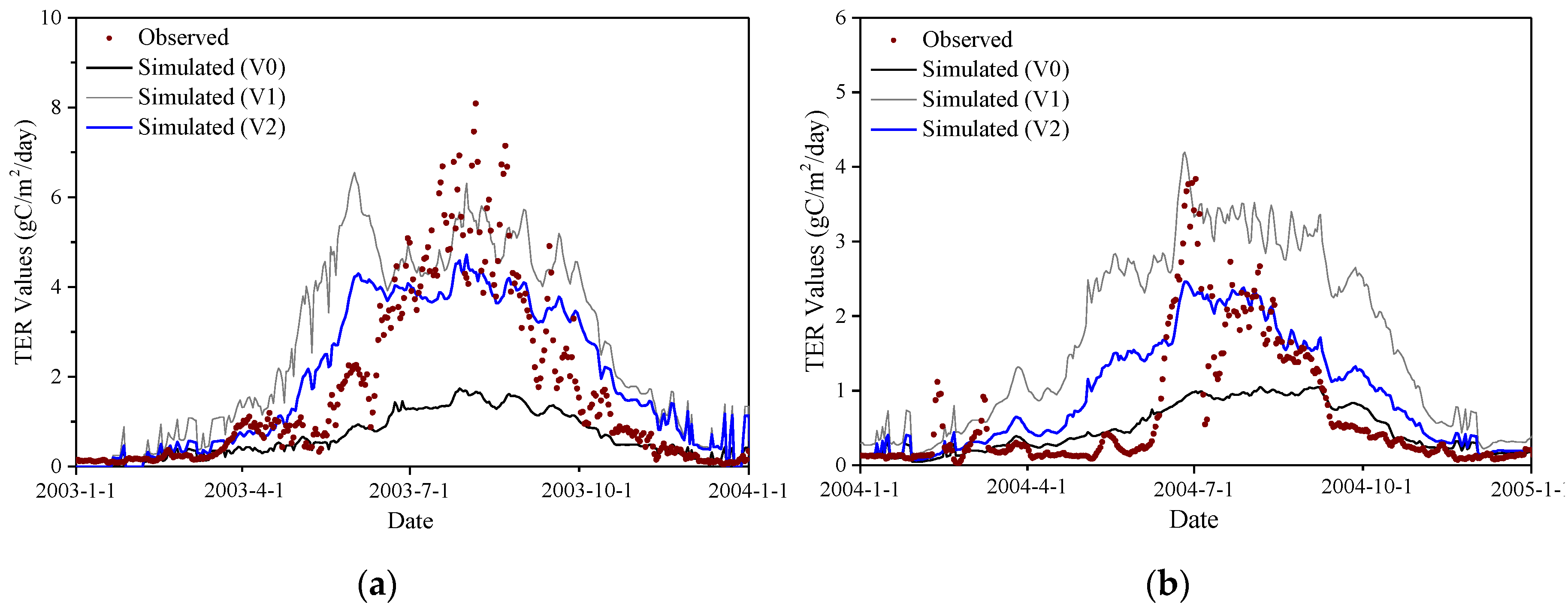
On the other hand, we also used EC-measured NEE and total ecosystem respiration (TER) to validate the performance of V2. As can be seen from Figure 5 and Figure S4, compared with V0 and V1, V2 significantly improved the simulation accuracy of NEE during the growing season at both Haibei Station and Damxung Station. However, it should be noted that there were still some discrepancies between the NEE simulated by V2 and the NEE measured by EC technique during the non-growing season, which may be attributed to the limitations in the soil respiration module of the Biome-BGC. In addition, as shown in Figure 6 and Figure S5, V2 also greatly improved the simulation accuracy of TER, which generated a good agreement with the observed TER. Overall, the Biome-BGC model, after a phenology module modification and parameter calibration, effectively improved the simulation accuracy of carbon fluxes and had a good consistency with the observations, which can be used for GPP simulation of alpine grasslands on the TP.
4.4. Spatial Patterns and Trends of GPP
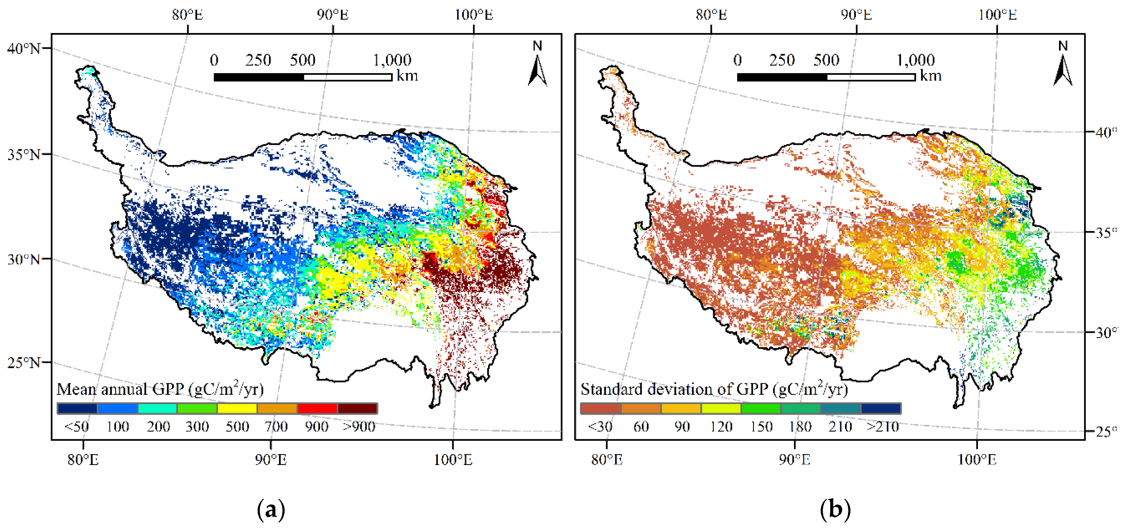
Based on V2, we simulated the GPP of alpine grasslands on the TP from 1982 to 2015. The spatial pattern of mean annual GPP and its standard deviation (sd) were shown in Figure 7. Generally, the mean annual GPP (Figure 7a) gradually decreased from southeast to northwest, consistent with the hydrothermal gradient of the TP. At the same time, the sd of GPP (Figure 7b) showed a decreasing trend from east to west, indicating that GPP in the eastern region has experienced greater fluctuations than GPP in the western region in the past 34 years. According to the statistical results, the mean annual GPP of alpine grasslands on the TP was 289.8 gC/m2/yr (305.8 TgC/yr), of which alpine meadows and alpine steppes accounted for 461.6 gC/m2/yr and 87.9 gC/m2/yr, respectively. In addition, most regions (65.3% of the alpine grassland area) had low sd of GPP within 60 gC/m2/yr over the study period, mainly distributed in the western region of the TP. Meanwhile, only 12.4% of the alpine grassland areas had sd greater than 120 gC/m2/yr, mainly located in the eastern region of the TP.
The spatial distribution of the trends of GPP between 1982 and 2015 was provided in Figure 8. Obviously, the GPP trends on the TP showed a large spatial heterogeneity, which may be mainly attributable to the different changes in climatic conditions. Overall, the mean annual GPP in most regions (96.5%) showed an increasing trend, with 63.5% of the alpine grassland area increasing significantly. This trend was also reflected in its interannual variations (Figure 9a). As depicted, the mean annual GPP increased significantly from 1982 to 2015, with a rate of 2.91 gC/m2/yr, and it varied from 250.9 gC/m2/yr in 1982 to 347.5 gC/m2/yr in 2015. Meanwhile, its changing trend was closely related to the changes in precipitation and temperature, as shown in Figure 9b,c. In addition, it should be noted that the mean annual GPP in 1998 had a significant increase as compared to the mean annual GPP of the previous year. This anomaly may be attributed to the EI Nino and La Nina events in 1998. Specifically, the average temperature and precipitation in 1998 were obviously higher than those in 1997, and the SOS of most alpine grasslands was also advanced [23], all of which directly contributed to the significant increase of GPP in 1998.
5. Discussion
5.1. The Role of Remotely Sensed Phenology in the Biome-BGC Model
Vegetation phenology strongly influences energy, carbon, and nitrogen cycling between the atmosphere and the terrestrial ecosystems. Accurate phenology simulation is a prerequisite for the accurate simulation of carbon fluxes. As mentioned earlier, the original meteorological-based phenology module in the Biome-BGC was found to significantly delay the SOS of alpine grasslands, which seriously affected the simulation accuracy of GPP. This limitation has also been discovered by [21], and its reason may be attributed to the fact that the moisture threshold and the temperature threshold in the original meteorological-based phenology module are not applicable to alpine regions like the TP. Specifically, the meteorological-based phenology module in the Biome-BGC assumes that leaf onset occurs when both the summed soil temperature and the summed precipitation are greater than the critical values [22]. However, for the TP, the seasonal thawing of frozen soil and snow cover can provide water for the germination and growth of alpine vegetation, which will make the original moisture threshold become inapplicable. Furthermore, the temperature threshold in the original phenology module of the Biome-BGC was derived from the empirical data for well-suited regions, which may also not well represent the vegetation growth on the TP. Therefore, improvements to the phenology module of the Biome-BGC is required.
Due to the temporal and spatial continuity of remote sensing technology, it has been successfully used for the study of vegetation phenology on the TP [25,26]. In this study, we have used the remotely sensed phenology to prescribe the phenological states within the Biome-BGC model. Results show that the remotely sensed phenology can more accurately represent the phenological characteristics of alpine grasslands than the original meteorological-based phenology module in the Biome-BGC. In addition, different from the previous studies that improved the phenology module of the Biome-BGC [19,20], our study integrated the remotely sensed phenology with the Biome-BGC model, which is more suitable for applications over large areas. This strategy could also be extended to other process-based ecosystem models. However, some limitations of this strategy should also be mentioned. Because remote sensing is an earth observation technique, it can only observe vegetation phenology in a hindcasting manner. Therefore, the Biome-BGC model after a phenology module modification in this study is incapable of making future predictions based on future climate scenarios. At the same time, since NDVI is not sensitive to seasonal changes in most evergreens, this strategy is also not applicable to evergreen species. On the other hand, it is worth mentioning that Sun et al. [63] proposed a multi-factor-driven prognostic phenology module for alpine meadows by combining temperature, precipitation, photoperiod, insolation, and snowfall, which could also be integrated into the Biome-BGC model to overcome the limitations in its original phenology module.
5.2. Performance of the Calibrated Biome-BGC Model
Model parameter calibration has long been considered as a difficult task, especially for complex process-based ecosystem models such as the Biome-BGC. In this study, we proposed a practical method for model calibration by combining a global sensitivity analysis with the simulated annealing optimization algorithm. The calibration results show that the carbon fluxes simulated by the calibrated Biome-BGC model are in good agreement with the EC measurements. However, it should be noted that the NEE simulated by the calibrated model is still overestimated during the non-growing season, and its reason can be traced back to the overestimation of TER. Furthermore, the overestimation of TER can be largely attributed to the soil respiration simulation, which is the main source of respired carbon during the non-growing season. The problem of soil respiration module in the Biome-BGC has also been reported in previous studies [17,19,64], and its reason was attributed to either the flaw in the respiration algorithm or the oversimplified simulation of soil temperature [19]. Nevertheless, for the TP, the problem of soil respiration module may also be attributed to the widespread distribution of frozen soil in the non-growing season. Specifically, the presence of frozen soil usually has a large impact on soil temperature, which will further affect the activity of soil microbes and ultimately act on soil respiration. Another study conducted on the TP has also demonstrated the important effects of frozen soil on soil respiration during the non-growing season [65].
On the other hand, some problems regarding model parameter calibration by numerical inversion methods must be acknowledged. Since the mathematical methods used to estimate model parameters usually treat the model as a “black box”, that is, the calibration procedure is only based on mathematical optimization criteria without considering the physiological processes within the model, so the calibrated results may not be true [20]. Therefore, some studies suggest avoiding the use of mathematical methods for model calibration and instead using field measurements to determine parameter values [66]. However, for complex process-based ecosystem models like the Biome-BGC, it usually contains a large number of tunable parameters (e.g., 28 ecophysiological parameters for the Biome-BGC), which means that it is almost impossible to obtain all (or even some specific) model parameters through field measurements, especially for applications over large areas. Admittedly, we can choose a subset of parameters for observation, but considering the correlation between model parameters and the large difference in the sensitivity of the parameters to the model output [61], it is still a difficult task, especially when some parameters cannot be observed directly. Therefore, in the absence of alternatives, combining sensitivity analysis with numerical inversion methods for model calibration is still a relatively feasible and reliable approach, which is also the method used in this study.
5.3. Uncertainties and Limitations
The spatial pattern of GPP of alpine grasslands on the TP exhibited obvious spatial heterogeneity in our study (Figure 7), consistent with other studies revealed that the GPP of Tibetan alpine grasslands showed a decreasing trend from southeast to northwest [14,16]. In addition, the mean annual GPP of Tibetan alpine grasslands from 2003 to 2008 simulated by [14] using a modified VPM model was 312.3 gC/m2/yr, which is slightly lower than the GPP (317.1 gC/m2/yr) simulated by our study during the same period, and this small discrepancy may be attributable to the differences in the model used.
On the other hand, some uncertainties still remain in our simulation of the carbon fluxes based on the improved Biome-BGC model. Firstly, since we used the EC-derived GPP data to calibrate the Biome-BGC model, which is essentially obtained through flux partitioning rather than direct observation, the GPP data will inevitably have errors and will further bring uncertainty to the model calibration and GPP simulation. Secondly, disturbances in human activities such as grazing and land use changes can also lead to bias in the GPP simulation. Thirdly, the NDVI dataset used to determine the phenology metrics may also bring uncertainty to the GPP simulation. Specifically, some studies reported that newly launched sensors such as MODIS have better performance than AVHRR for determining phenological parameters in alpine regions [24,67,68]. However, MODIS data was not available until 2000, so we chose to use a single data source to extract phenological parameters to avoid new uncertainties caused by the combination of different sensors. In addition, it is worth mentioning that Kern et al. [69] have improved the quality of GIMMS NDVI3g dataset by applying a local correction to the NDVI3g dataset using MODIS NDVI, which could also be considered in our future work. Finally, uncertainties may also come from the internal structure of the Biome-BGC model. Specifically, due to the widespread distribution of frozen soil on the TP, they will have an important impact on the physiological processes of alpine grasslands, which in turn will affect the carbon cycle and energy flow of alpine grassland ecosystems [25,70]. However, the existence of frozen soil and its effects on the physiological processes have not been considered in the Biome-BGC model, so further improvements to the model structure are still needed. On the other hand, it is worth mentioning that some already improved versions of the Biome-BGC model could also be considered in our future work to reconcile the above issues. For example, Hidy et al. [71] obtained an improved Biome-BGC model (referred to as the Biome-BGCMuSo) by adding a multilayer soil module and a management module to the original model, which could help with the issue of frozen soil and human activities.
6. Conclusions
In view of the limitations of the Biome-BGC model when applied to alpine regions, we have prescribed its phenological states based upon the remotely sensed phenology and calibrated its parameters to improve the modeling of GPP of alpine grasslands on the Tibetan Plateau (TP). Specifically, we first used the remotely sensed phenology to modify the original meteorological-based phenology module in the Biome-BGC to better prescribe the phenological states within the model, and then we combined the global sensitivity analysis method with the simulated annealing algorithm to calibrate the model parameters. Furthermore, we used the improved Biome-BGC model to simulate the GPP of alpine grasslands on the TP from 1982 to 2015. The results show that the improved Biome-BGC model effectively overcame the limitations in the original model and was capable of reproducing the magnitude and the temporal dynamics of GPP of alpine grasslands. At the same time, the simulated results indicate that the GPP of alpine grasslands on the TP exhibited a large spatial heterogeneity, which generally showed a decreasing trend from southeast to northwest and was consistent with the hydrothermal gradient of the TP. In addition, the mean annual GPP of alpine grasslands on the TP from 1982 to 2015 estimated by our study was 289.8 gC/m2/yr (305.8 TgC/yr), and GPP in most regions showed a significant increasing trend. However, it should be noted that although GPP exhibits an increasing trend over the past 34 years, the general trend in net carbon uptake is still unclear given the large uncertainty in soil respiration during the non-growing season. Therefore, in the case that more field-measured data such as soil temperature is available, we also need to consider the effects of frozen soil on alpine vegetation and further improve the soil respiration module of the Biome-BGC to obtain the carbon budget dynamics of alpine grassland ecosystem on the TP.
Supplementary Materials
The following are available online at https://www.mdpi.com/2072-4292/11/11/1287/s1. A detailed description of the Morris method, Figure S1: Morris sensitivity indices of mean annual GPP to the input ecophysiological parameters; Figure S2: Sobol’ sensitivity indices of mean annual GPP to the input ecophysiological parameters screened by the Morris method; Figure S3: Comparisons between GPP derived from EC measurements and GPP simulated by the version of V0, V1, and V2 for the validation year; Figure S4: Comparisons between NEE measured by EC technique and NEE simulated by the version of V0, V1, and V2 for the validation year; Figure S5: Comparisons between TER derived from EC measurements and TER simulated by the version of V0, V1, and V2 for the validation year.
Author Contributions
Y.Y. and S.W. conceived and designed the method and the experiments, and led the manuscript writing; Y.Y. and S.W. conducted the experiments and analyzed the data; Y.M., X.W., and W.L. provided help and suggestions in the experiments and its interpretation; Y.M. and X.W. contributed to the writing and revision of the manuscript.
Funding
This research was funded by the Strategic Priority Research Program of the Chinese Academy of Sciences: CAS Earth Big Data Science Project (No. XDA19030501), the Second Comprehensive Scientific Investigation of the Tibetan Plateau: Aerial Water Resources Monitoring on the Tibetan Plateau based on the Space-Air-Ground Integrated Network (No. 2019QZKK0204), and the National Natural Science Foundation of China (Nos. 91547107, 41271426, and 41428103).
Acknowledgments
The EC data used in this study is provided by the Chinese Flux Observation and Research Network, and the China Meteorological Forcing Dataset is developed by Data Assimilation and Modeling Center for Tibetan Multi-spheres, Institute of Tibetan Plateau Research, Chinese Academy of Sciences. The authors are very grateful for Yaoming Ma, Institute of Tibetan Plateau Research, Chinese Academy of Sciences, for his help in acquiring the EC data. The authors also want to show their gratitude to the anonymous reviewers and the editors for their insightful and valuable comments.
Conflicts of Interest
The authors declare no conflict of interest.
References
- Running, S.W.; Nemani, R.R.; Heinsch, F.A.; Zhao, M.S.; Reeves, M.; Hashimoto, H. A continuous satellite-derived measure of global terrestrial primary production. Bioscience 2004, 54, 547–560. [Google Scholar] [CrossRef]
- Gitelson, A.A.; Vina, A.; Verma, S.B.; Rundquist, D.C.; Arkebauer, T.J.; Keydan, G.; Leavitt, B.; Ciganda, V.; Burba, G.G.; Suyker, A.E. Relationship between gross primary production and chlorophyll content in crops: Implications for the synoptic monitoring of vegetation productivity. J. Geophys. Res. Atmos. 2006, 111, D08S11. [Google Scholar] [CrossRef]
- Beer, C.; Reichstein, M.; Tomelleri, E.; Ciais, P.; Jung, M.; Carvalhais, N.; Rodenbeck, C.; Arain, M.A.; Baldocchi, D.; Bonan, G.B.; et al. Terrestrial Gross Carbon Dioxide Uptake: Global Distribution and Covariation with Climate. Science 2010, 329, 834–838. [Google Scholar] [CrossRef] [PubMed] [Green Version]
- Tan, K.; Ciais, P.; Piao, S.L.; Wu, X.P.; Tang, Y.H.; Vuichard, N.; Liang, S.; Fang, J.Y. Application of the ORCHIDEE global vegetation model to evaluate biomass and soil carbon stocks of Qinghai-Tibetan grasslands. Glob. Biogeochem. Cycles 2010, 24, GB1013. [Google Scholar] [CrossRef]
- Piao, S.L.; Ciais, P.; Huang, Y.; Shen, Z.H.; Peng, S.S.; Li, J.S.; Zhou, L.P.; Liu, H.Y.; Ma, Y.C.; Ding, Y.H.; et al. The impacts of climate change on water resources and agriculture in China. Nature 2010, 467, 43–51. [Google Scholar] [CrossRef]
- Piao, S.L.; Tan, K.; Nan, H.J.; Ciais, P.; Fang, J.Y.; Wang, T.; Vuichard, N.; Zhu, B.A. Impacts of climate and CO2 changes on the vegetation growth and carbon balance of Qinghai-Tibetan grasslands over the past five decades. Glob. Planet. Chang. 2012, 98, 73–80. [Google Scholar] [CrossRef]
- Wylie, B.K.; Fosnight, E.A.; Gilmanov, T.G.; Frank, A.B.; Morgan, J.A.; Haferkamp, M.R.; Meyers, T.P. Adaptive data-driven models for estimating carbon fluxes in the Northern Great Plains. Remote Sens. Environ. 2007, 106, 399–413. [Google Scholar] [CrossRef] [Green Version]
- Veroustraete, F.; Sabbe, H.; Eerens, H. Estimation of carbon mass fluxes over Europe using the C-Fix model and Euroflux data. Remote Sens. Environ. 2002, 83, 376–399. [Google Scholar] [CrossRef]
- Xiao, X.M.; Hollinger, D.; Aber, J.; Goltz, M.; Davidson, E.A.; Zhang, Q.Y.; Moore, B. Satellite-based modeling of gross primary production in an evergreen needleleaf forest. Remote Sens. Environ. 2004, 89, 519–534. [Google Scholar] [CrossRef]
- Melillo, J.M.; McGuire, A.D.; Kicklighter, D.W.; Moore, B.; Vorosmarty, C.J.; Schloss, A.L. Global climate-change and terrestrial net primary production. Nature 1993, 363, 234–240. [Google Scholar] [CrossRef]
- Running, S.W.; Hunt, E.R. Generalization of a Forest Ecosystem Process Model for Other Biomes, BIOME-BGC, and an Application for Global-Scale Models. In Scaling Physiological Processes; Ehleringer, J.R., Field, C.B., Eds.; Academic Press: San Diego, CA, USA, 1993; pp. 141–158. [Google Scholar]
- Krinner, G.; Viovy, N.; de Noblet-Ducoudre, N.; Ogee, J.; Polcher, J.; Friedlingstein, P.; Ciais, P.; Sitch, S.; Prentice, I.C. A dynamic global vegetation model for studies of the coupled atmosphere-biosphere system. Glob. Biogeochem. Cycles 2005, 19, GB1015. [Google Scholar] [CrossRef]
- Zhuang, Q.; He, J.; Lu, Y.; Ji, L.; Xiao, J.; Luo, T. Carbon dynamics of terrestrial ecosystems on the Tibetan Plateau during the 20th century: An analysis with a process-based biogeochemical model. Glob. Ecol. Biogeogr. 2010, 19, 649–662. [Google Scholar] [CrossRef]
- He, H.L.; Liu, M.; Xiao, X.M.; Ren, X.L.; Zhang, L.; Sun, X.M.; Yang, Y.H.; Li, Y.N.; Zhao, L.; Shi, P.L.; et al. Large-scale estimation and uncertainty analysis of gross primary production in Tibetan alpine grasslands. J. Geophys. Res. Biogeosci. 2014, 119, 466–486. [Google Scholar] [CrossRef] [Green Version]
- Ma, M.N.; Yuan, W.P.; Dong, J.; Zhang, F.W.; Cai, W.W.; Li, H.Q. Large-scale estimates of gross primary production on the Qinghai-Tibet plateau based on remote sensing data. Int. J. Digit Earth 2018, 11, 1166–1183. [Google Scholar] [CrossRef]
- Chen, S.; Huang, Y.; Gao, S.; Wang, G. Impact of physiological and phenological change on carbon uptake on the Tibetan Plateau revealed through GPP estimation based on spaceborne solar-induced fluorescence. Sci. Total Environ. 2019, 663, 45–59. [Google Scholar] [CrossRef] [PubMed]
- Thornton, P.E.; Law, B.E.; Gholz, H.L.; Clark, K.L.; Falge, E.; Ellsworth, D.S.; Golstein, A.H.; Monson, R.K.; Hollinger, D.; Falk, M.; et al. Modeling and measuring the effects of disturbance history and climate on carbon and water budgets in evergreen needleleaf forests. Agric. For. Meteorol. 2002, 113, 185–222. [Google Scholar] [CrossRef]
- Chiesi, M.; Maselli, F.; Moriondo, M.; Fibbi, L.; Bindi, M.; Running, S.W. Application of BIOME-BGC to simulate Mediterranean forest processes. Ecol. Model. 2007, 206, 179–190. [Google Scholar] [CrossRef]
- Mao, F.J.; Li, P.H.; Zhou, G.M.; Du, H.Q.; Xu, X.J.; Shi, Y.J.; Mo, L.F.; Zhou, Y.F.; Tu, G.Q. Development of the BIOME-BGC model for the simulation of managed Moso bamboo forest ecosystems. J. Environ. Manag. 2016, 172, 29–39. [Google Scholar] [CrossRef]
- Hidy, D.; Barcza, Z.; Haszpra, L.; Churkina, G.; Pinter, K.; Nagy, Z. Development of the Biome-BGC model for simulation of managed herbaceous ecosystems. Ecol. Model. 2012, 226, 99–119. [Google Scholar] [CrossRef]
- Sun, Q.; Li, B.; Zhang, T.; Yuan, Y.; Gao, X.; Ge, J.; Li, F.; Zhang, Z. An improved Biome-BGC model for estimating net primary productivity of alpine meadow on the Qinghai-Tibet Plateau. Ecol. Model. 2017, 350, 55–68. [Google Scholar] [CrossRef]
- White, M.A.; Thornton, P.E.; Running, S.W. A continental phenology model for monitoring vegetation responses to interannual climatic variability. Glob. Biogeochem. Cycles 1997, 11, 217–234. [Google Scholar] [CrossRef]
- Wang, S.; Wang, X.; Chen, G.; Yang, Q.; Wang, B.; Ma, Y.; Shen, M. Complex responses of spring alpine vegetation phenology to snow cover dynamics over the Tibetan Plateau, China. Sci. Total Environ. 2017, 593, 449–461. [Google Scholar] [CrossRef] [PubMed]
- Zhang, G.L.; Zhang, Y.J.; Dong, J.W.; Xiao, X.M. Green-up dates in the Tibetan Plateau have continuously advanced from 1982 to 2011. Proc. Natl. Acad. Sci. USA 2013, 110, 4309–4314. [Google Scholar] [CrossRef] [Green Version]
- Wang, S.; Zhang, B.; Yang, Q.; Chen, G.; Yang, B.; Lu, L.; Shen, M.; Peng, Y. Responses of net primary productivity to phenological dynamics in the Tibetan Plateau, China. Agric. For. Meteorol. 2017, 232, 235–246. [Google Scholar] [CrossRef]
- Wang, X.; Wu, C.; Peng, D.; Gonsamo, A.; Liu, Z. Snow cover phenology affects alpine vegetation growth dynamics on the Tibetan Plateau: Satellite observed evidence, impacts of different biomes, and climate drivers. Agric. For. Meteorol. 2018, 256, 61–74. [Google Scholar] [CrossRef]
- Arora, V.K.; Boer, G.J. A parameterization of leaf phenology for the terrestrial ecosystem component of climate models. Glob. Chang. Biol. 2005, 11, 39–59. [Google Scholar] [CrossRef]
- Gonsamo, A.; Chen, J.M.; Price, D.T.; Kurz, W.A.; Liu, J.; Boisvenue, C.; Hember, R.A.; Wu, C.Y.; Chang, K.H. Improved assessment of gross and net primary productivity of Canada’s landmass. J. Geophys. Res. Biogeosci. 2013, 118, 1546–1560. [Google Scholar] [CrossRef]
- Wang, J.; Wu, C.Y.; Zhang, C.H.; Ju, W.M.; Wang, X.Y.; Chen, Z.; Fang, B. Improved modeling of gross primary productivity (GPP) by better representation of plant phenological indicators from remote sensing using a process model. Ecol. Indic. 2018, 88, 332–340. [Google Scholar] [CrossRef]
- Zheng, D.; Lin, Z.Y.; Zhang, X.Q. Progress in studies of Tibetan Plateau and global environmental change. Earth Sci. Front. 2002, 9, 95–102. [Google Scholar]
- Chen, X.Q.; An, S.; Inouye, D.W.; Schwartz, M.D. Temperature and snowfall trigger alpine vegetation green-up on the world’s roof. Glob. Chang. Biol. 2015, 21, 3635–3646. [Google Scholar] [CrossRef]
- Ni, J. Carbon storage in grasslands of China. J. Arid Environ. 2002, 50, 205–218. [Google Scholar] [CrossRef]
- Hungerford, D.R.; Nemani, R.; Running, W.S.; Coughlan, C.J. MT-CLIM: A Mountain Microclimate Simulation Model; US Department of Agriculture, Forest Service, Intermountain Research Station: Ogden, UT, USA, 1989.
- Yu, G.R.; Wen, X.F.; Sun, X.M.; Tanner, B.D.; Lee, X.H.; Chen, J.Y. Overview of ChinaFLUX and evaluation of its eddy covariance measurement. Agric. For. Meteorol. 2006, 137, 125–137. [Google Scholar] [CrossRef]
- Li, C.; He, H.L.; Liu, M.; Su, W.; Fu, Y.L.; Zhang, L.M.; Wen, X.F.; Yu, G.R. The design and application of CO2 flux data processing system at ChinaFLUX. Geo-Inf. Sci. 2008, 10, 557–565. (In Chinese) [Google Scholar]
- Falge, E.; Baldocchi, D.; Olson, R.; Anthoni, P.; Aubinet, M.; Bernhofer, C.; Burba, G.; Ceulemans, G.; Clement, R.; Dolman, H.; et al. Gap filling strategies for long term energy flux data sets. Agric. For. Meteorol. 2001, 107, 71–77. [Google Scholar] [CrossRef] [Green Version]
- Lloyd, J.; Taylor, J.A. On the temperature-dependence of soil respiration. Funct. Ecol. 1994, 8, 315–323. [Google Scholar] [CrossRef]
- Wang, B. Study on Carbon Flux and Its Controlling Mechanisms in a Degraded Alpine Meadow and an Artificial Pasture in the Three-River Source Region of the Qinghai-Tibetan Plateau; Nankai University: Tianjin, China, 2014. [Google Scholar]
- White, M.A.; Thornton, P.E.; Running, S.W.; Nemani, R.R. Parameterization and sensitivity analysis of the BIOME–BGC terrestrial ecosystem model: Net primary production controls. Earth Interact. 2000, 4, 1–85. [Google Scholar] [CrossRef]
- Tucker, C.J. Red and photographic infrared linear combinations for monitoring vegetation. Remote Sens. Environ. 1979, 8, 127–150. [Google Scholar] [CrossRef] [Green Version]
- Chang, Q.; Zhang, J.H.; Jiao, W.Z.; Yao, F.M. A comparative analysis of the NDVIg and NDVI3g in monitoring vegetation phenology changes in the Northern Hemisphere. Geocarto Int. 2016, 33, 1–20. [Google Scholar] [CrossRef]
- Zhu, Z.C.; Bi, J.; Pan, Y.Z.; Ganguly, S.; Anav, A.; Xu, L.; Samanta, A.; Piao, S.L.; Nemani, R.R.; Myneni, R.B. Global Data Sets of Vegetation Leaf Area Index (LAI)3g and Fraction of Photosynthetically Active Radiation (FPAR)3g Derived from Global Inventory Modeling and Mapping Studies (GIMMS) Normalized Difference Vegetation Index (NDVI3g) for the Period 1981 to 2011. Remote Sens. 2013, 5, 927–948. [Google Scholar] [CrossRef] [Green Version]
- Holben, B.N. Characteristics of maximum-value composite images from temporal avhrr data. Int. J. Remote Sens. 1986, 7, 1417–1434. [Google Scholar] [CrossRef]
- Chen, J.; Jonsson, P.; Tamura, M.; Gu, Z.H.; Matsushita, B.; Eklundh, L. A simple method for reconstructing a high-quality NDVI time-series data set based on the Savitzky-Golay filter. Remote Sens. Environ. 2004, 91, 332–344. [Google Scholar] [CrossRef]
- Running, S.W.; Coughlan, J.C. A general-model of forest ecosystem processes for regional applications I. hydrologic balance, canopy gas-exchange and primary production processes. Ecol. Model. 1988, 42, 125–154. [Google Scholar] [CrossRef]
- Yan, M.; Tian, X.; Li, Z.Y.; Chen, E.X.; Wang, X.F.; Han, Z.T.; Sun, H. Simulation of Forest Carbon Fluxes Using Model Incorporation and Data Assimilation. Remote Sens. 2016, 8, 567. [Google Scholar] [CrossRef]
- Farquhar, G.D.; von Caemmerer, S.; Berry, J.A. A biochemical model of photosynthetic CO2 assimilation in leaves of C3 species. Planta. 1980, 149, 78–90. [Google Scholar] [CrossRef]
- dePury, D.G.G.; Farquhar, G.D. Simple scaling of photosynthesis from leaves to canopies without the errors of big-leaf models. Plant Cell Environ. 1997, 20, 537–557. [Google Scholar] [CrossRef]
- Richardson, A.D.; Anderson, R.S.; Arain, M.A.; Barr, A.G.; Bohrer, G.; Chen, G.S.; Chen, J.M.; Ciais, P.; Davis, K.J.; Desai, A.R.; et al. Terrestrial biosphere models need better representation of vegetation phenology: Results from the North American Carbon Program Site Synthesis. Glob. Chang. Biol. 2012, 18, 566–584. [Google Scholar] [CrossRef]
- Burgan, R.E.; Hartford, R.A. Monitoring Vegetation Greenness with Satellite Data; Gen. Tech. Rep. INT-GTR-297; US Department of Agriculture, Forest Service, Intermountain Research Station: Ogden, UT, USA, 1993; Volume 297, p. 13.
- Zhang, X.; Friedl, M.A.; Schaaf, C.B.; Strahler, A.H.; Hodges, J.C.; Gao, F.; Reed, B.C.; Huete, A. Monitoring vegetation phenology using MODIS. Remote Sens. Environ. 2003, 84, 471–475. [Google Scholar] [CrossRef]
- Kaduk, J.; Heimann, M. A prognostic phenology scheme for global terrestrial carbon cycle models. Clim. Res. 1996, 6, 1–19. [Google Scholar] [CrossRef]
- Reed, B.C.; Brown, J.F.; Vanderzee, D.; Loveland, T.R.; Merchant, J.W.; Ohlen, D.O. Measuring phenological variability from satellite imagery. J. Veg. Sci. 1994, 5, 703–714. [Google Scholar] [CrossRef]
- Richardson, A.D.; Black, T.A.; Ciais, P.; Delbart, N.; Friedl, M.A.; Gobron, N.; Hollinger, D.Y.; Kutsch, W.L.; Longdoz, B.; Luyssaert, S.; et al. Influence of spring and autumn phenological transitions on forest ecosystem productivity. Philos. Trans. R. Soc. B-Biol. Sci. 2010, 365, 3227–3246. [Google Scholar] [CrossRef] [PubMed] [Green Version]
- Hufkens, K.; Friedl, M.; Sonnentag, O.; Braswell, B.H.; Milliman, T.; Richardson, A.D. Linking near-surface and satellite remote sensing measurements of deciduous broadleaf forest phenology. Remote Sens. Environ. 2012, 117, 307–321. [Google Scholar] [CrossRef]
- Saltelli, A.; Tarantola, S.; Campolongo, F.; Ratto, M. Sensitivity Analysis in Practice: A Guide to Assessing Scientific Models; John Wiley & Sons: Chichester, England, 2004. [Google Scholar]
- Morris, M.D. Factorial sampling plans for preliminary computational experiments. Technometrics 1991, 33, 161–174. [Google Scholar] [CrossRef]
- Sobol, I.M. Sensitivity estimates for nonlinear mathematical models. Math. Model. Comput. Exp. 1993, 1, 407–414. [Google Scholar]
- Metropolis, N.; Ulam, S. The monte carlo method. J. Am. Stat. Assoc. 1949, 44, 335–341. [Google Scholar] [CrossRef] [PubMed]
- Kirkpatrick, S.; Gelatt, C.D.; Vecchi, M.P. OPTIMIZATION BY SIMULATED ANNEALING. Science 1983, 220, 671–680. [Google Scholar] [CrossRef]
- Wang, W.; Ichii, K.; Hashimoto, H.; Michaelis, A.R.; Thornton, P.E.; Law, B.E.; Nemani, R.R. A hierarchical analysis of terrestrial ecosystem model Biome-BGC: Equilibrium analysis and model calibration. Ecol. Model. 2009, 220, 2009–2023. [Google Scholar] [CrossRef]
- Churkina, G.; Brovkin, V.; von Bloh, W.; Trusilova, K.; Jung, M.; Dentener, F. Synergy of rising nitrogen depositions and atmospheric CO2 on land carbon uptake moderately offsets global warming. Glob. Biogeochem. Cycles 2009, 23. [Google Scholar] [CrossRef]
- Sun, Q.L.; Li, B.L.; Yuan, Y.C.; Jiang, Y.H.; Zhang, T.; Gao, X.Z.; Ge, J.S.; Li, F.; Zhang, Z.J. A prognostic phenology model for alpine meadows on the Qinghai-Tibetan Plateau. Ecol. Indic. 2018, 93, 1089–1100. [Google Scholar] [CrossRef]
- Aguilos, M.; Takagi, K.; Liang, N.; Ueyama, M.; Fukuzawa, K.; Nomura, M.; Kishida, O.; Fukazawa, T.; Takahashi, H.; Kotsuka, C.; et al. Dynamics of ecosystem carbon balance recovering from a clear-cutting in a cool-temperate forest. Agric. For. Meteorol. 2014, 197, 26–39. [Google Scholar] [CrossRef] [Green Version]
- Wang, Y.H.; Liu, H.Y.; Chung, H.; Yu, L.F.; Mi, Z.R.; Geng, Y.; Jing, X.; Wang, S.P.; Zeng, H.; Cao, G.M.; et al. Non-growing-season soil respiration is controlled by freezing and thawing processes in the summer monsoon-dominated Tibetan alpine grassland. Glob. Biogeochem. Cycles 2014, 28, 1081–1095. [Google Scholar] [CrossRef]
- Makela, A.; Valentine, H.T. The ratio of NPP to GPP: Evidence of change over the course of stand development. Tree Physiol. 2001, 21, 1015–1030. [Google Scholar] [CrossRef]
- Fontana, F.; Rixen, C.; Jonas, T.; Aberegg, G.; Wunderle, S. Alpine grassland phenology as seen in AVHRR, VEGETATION, and MODIS NDVI time series—A comparison with in situ measurements. Sensors 2008, 8, 2833–2853. [Google Scholar] [CrossRef] [PubMed]
- Zeng, H.Q.; Jia, G.S.; Epstein, H. Recent changes in phenology over the northern high latitudes detected from multi-satellite data. Environ. Res. Lett. 2011, 6, 045508. [Google Scholar] [CrossRef] [Green Version]
- Kern, A.; Marjanovic, H.; Barcza, Z. Evaluation of the Quality of NDVI3g Dataset against Collection 6 MODIS NDVI in Central Europe between 2000 and 2013. Remote Sens. 2016, 8, 955. [Google Scholar] [CrossRef]
- Li, W.; Wu, J.; Bai, E.; Jin, C.; Wang, A.; Yuan, F.; Guan, D. Response of terrestrial carbon dynamics to snow cover change: A meta-analysis of experimental manipulation (II). Soil Biol. Biochem. 2016, 103, 388–393. [Google Scholar] [CrossRef]
- Hidy, D.; Barcza, Z.; Marjanovic, H.; Sever, M.Z.O.; Dobor, L.; Gelybo, G.; Fodor, N.; Pinter, K.; Churkina, G.; Running, S.; et al. Terrestrial ecosystem process model Biome-BGCMuSo v4.0: Summary of improvements and new modeling possibilities. Geosci. Model. Dev. 2016, 9, 4405–4437. [Google Scholar] [CrossRef]
Figure 1.
Spatial distributions of grassland subtypes and elevations on the Tibetan Plateau (TP). (a) Grassland subtypes; (b) Elevation.
Figure 1.
Spatial distributions of grassland subtypes and elevations on the Tibetan Plateau (TP). (a) Grassland subtypes; (b) Elevation.

Figure 2.
The flow chart of this study. EC, eddy covariance; GPP, gross primary productivity.

Figure 3.
Spatial distribution of phenological indicators of alpine grasslands on the TP. (a) The start of growing season (SOS); (b) The end of growing season (EOS); (c) The length of growing season (LOS).
Figure 3.
Spatial distribution of phenological indicators of alpine grasslands on the TP. (a) The start of growing season (SOS); (b) The end of growing season (EOS); (c) The length of growing season (LOS).

Figure 4.
Comparisons between GPP derived from EC measurements and GPP simulated by the version of V0, V1, and V2 for the calibration year. (a) Haibei Station (alpine meadow); (b) Damxung Station (alpine steppe).
Figure 4.
Comparisons between GPP derived from EC measurements and GPP simulated by the version of V0, V1, and V2 for the calibration year. (a) Haibei Station (alpine meadow); (b) Damxung Station (alpine steppe).


Figure 5.
Comparisons between NEE measured by EC technique and NEE simulated by the version of V0, V1, and V2 for the calibration year. (a) Haibei Station (alpine meadow); (b) Damxung Station (alpine steppe).
Figure 5.
Comparisons between NEE measured by EC technique and NEE simulated by the version of V0, V1, and V2 for the calibration year. (a) Haibei Station (alpine meadow); (b) Damxung Station (alpine steppe).

Figure 6.
Comparisons between total ecosystem respiration (TER) derived from EC measurements and TER simulated by the version of V0, V1, and V2 for the calibration year. (a) Haibei Station (alpine meadow); (b) Damxung Station (alpine steppe).
Figure 6.
Comparisons between total ecosystem respiration (TER) derived from EC measurements and TER simulated by the version of V0, V1, and V2 for the calibration year. (a) Haibei Station (alpine meadow); (b) Damxung Station (alpine steppe).

Figure 7.
Spatial distribution of mean and standard deviation of GPP of alpine grasslands on the TP from 1982 to 2015. (a) Mean annual GPP; (b) Standard deviation of GPP.
Figure 7.
Spatial distribution of mean and standard deviation of GPP of alpine grasslands on the TP from 1982 to 2015. (a) Mean annual GPP; (b) Standard deviation of GPP.

Figure 8.
Spatial distribution of trends and significance levels of GPP of alpine grasslands on the TP from 1982 to 2015. (a) Trends of GPP; (b) Significance levels of GPP trends.
Figure 8.
Spatial distribution of trends and significance levels of GPP of alpine grasslands on the TP from 1982 to 2015. (a) Trends of GPP; (b) Significance levels of GPP trends.

Figure 9.
Interannual variations of different factors of alpine grasslands on the TP from 1982 to 2015. (a) Mean annual GPP; (b) Mean annual precipitation; (c) Mean annual temperature.
Figure 9.
Interannual variations of different factors of alpine grasslands on the TP from 1982 to 2015. (a) Mean annual GPP; (b) Mean annual precipitation; (c) Mean annual temperature.


Table 1.
Ecophysiological parameters of the Biome-BGC model for the type of C3 grass.
| No. | Ecophysiological Parameters | Symbol | Units 1 | PDF 2 | Source |
|---|---|---|---|---|---|
| 1 | Transfer growth period as fraction of growing season | TGGS | proportion | Wang [38] | |
| 2 | Litterfall as fraction of growing season | LGS | proportion | Sun et al. [21] | |
| 3 | Annual whole plant mortality fraction | WPM | 1/year | White et al. [39] | |
| 4 | Annual fire mortality fraction | FM | 1/year | / | / |
| 5 | New fine root C: new leaf C | FRC:LC | ratio | White et al. [39] | |
| 6 | Current growth proportion | CGP | proportion | White et al. [39] | |
| 7 | C:N ratio of leaves | C:Nleaf | kgC/kgN | White et al. [39] | |
| 8 | C:N ratio of leaf litter | C:Nlit | kgC/kgN | White et al. [39] | |
| 9 | C:N ratio of fine roots | C:Nfr | kgC/kgN | White et al. [39] | |
| 10 | Leaf litter labile proportion | Llab | DIM | 1-Lcel-Llig | / |
| 11 | Leaf litter cellulose proportion | Lcel | DIM | White et al. [39] | |
| 12 | Leaf litter lignin proportion | Llig | DIM | White et al. [39] | |
| 13 | Fine root labile proportion | FRlab | DIM | 1-FRcel-FRlig | / |
| 14 | Fine root cellulose proportion | FRcel | DIM | White et al. [39] | |
| 15 | Fine root lignin proportion | FRlig | DIM | White et al. [39] | |
| 16 | Canopy water interception coefficient | Wint | 1/LAI/day | White et al. [39] | |
| 17 | Canopy light extinction coefficient | LEC | DIM | White et al. [39] | |
| 18 | All-sided to projected leaf area ratio | LAIall:prj | DIM | White et al. [39] | |
| 19 | Canopy average specific leaf area | SLA | m2/kgC | White et al. [39] | |
| 20 | Ratio of shaded SLA: sunlit SLA | SLAsha:sun | DIM | White et al. [39] | |
| 21 | Percent of leaf N in Rubisco | PLNR | DIM | White et al. [39] | |
| 22 | Maximum stomatal conductance | Gsmax | m/s | White et al. [39] | |
| 23 | Cuticular conductance | Gcut | m/s | 0.01*Gsmax | / |
| 24 | Boundary layer conductance | Gbl | m/s | White et al. [39] | |
| 25 | Leaf water potential: start of conductance reduction | LWPi | MPa | White et al. [39] | |
| 26 | Leaf water potential: complete conductance reduction | LWPf | MPa | White et al. [39] | |
| 27 | Vapor pressure deficit: start of conductance reduction | VPDi | Pa | White et al. [39] | |
| 28 | Vapor pressure deficit: complete conductance reduction | VPDf | Pa | White et al. [39] |
1 DIM: dimensionless. 2 U(min, max): uniform distribution, N(mean, standard deviation): normal distribution. SLA, specific leaf area.
Table 2.
Descriptions of the two flux sites used in this study.
| Site | Grassland Subtype | Coordinate | Elevation | Canopy Height | Period |
|---|---|---|---|---|---|
| Haibei Station | Alpine Meadow | 37°37′N, 101°19′E | 3190 m | 0.2–0.3 m | 2003–2004 |
| Damxung Station | Alpine Steppe | 30°29′N, 91°04′E | 4330 m | <0.2 m | 2004–2005 |
Table 3.
The influential ecophysiological parameters and its calibrated values for Haibei Station and Damxung Station.
Table 3.
The influential ecophysiological parameters and its calibrated values for Haibei Station and Damxung Station.
| Influential Parameters 1 | Default Value | Calibrated Value | |
|---|---|---|---|
| Haibei Station | Damxung Station | ||
| FRC:LC | 2.0 | 2.07 | 1.94 |
| C:Nleaf | 24.0 | 32.93 | 35.04 |
| C:Nlit | 49.0 | 45.12 | 44.23 |
| C:Nfr | 42.0 | 43.66 | 35.42 |
| SLA | 45.0 | 44.39 | 44.61 |
| PLNR | 0.15 | 0.124 | 0.137 |
| Gsmax | 0.005 | 0.0025 | 0.0059 |
| LWPi | −0.6 | / 2 | −0.84 |
1 Influential parameters represent those parameters that have a significant impact on the GPP simulation and require calibration. They are a subset of ecophysiological parameters. 2 The backslash indicates that the parameter LWPi is insensitive to the GPP simulation at Haibei Station and is set to the default value.
© 2019 by the authors. Licensee MDPI, Basel, Switzerland. This article is an open access article distributed under the terms and conditions of the Creative Commons Attribution (CC BY) license (http://creativecommons.org/licenses/by/4.0/).
Share and Cite
MDPI and ACS Style
You, Y.; Wang, S.; Ma, Y.; Wang, X.; Liu, W. Improved Modeling of Gross Primary Productivity of Alpine Grasslands on the Tibetan Plateau Using the Biome-BGC Model. Remote Sens. 2019, 11, 1287. https://doi.org/10.3390/rs11111287
AMA Style
You Y, Wang S, Ma Y, Wang X, Liu W. Improved Modeling of Gross Primary Productivity of Alpine Grasslands on the Tibetan Plateau Using the Biome-BGC Model. Remote Sensing. 2019; 11(11):1287. https://doi.org/10.3390/rs11111287
Chicago/Turabian StyleYou, Yongfa, Siyuan Wang, Yuanxu Ma, Xiaoyue Wang, and Weihua Liu. 2019. "Improved Modeling of Gross Primary Productivity of Alpine Grasslands on the Tibetan Plateau Using the Biome-BGC Model" Remote Sensing 11, no. 11: 1287. https://doi.org/10.3390/rs11111287
Note that from the first issue of 2016, this journal uses article numbers instead of page numbers. See further details here.