Effects of the Temporal Aggregation and Meteorological Conditions on the Parameter Robustness of OCO-2 SIF-Based and LUE-Based GPP Models for Croplands

Abstract

Global retrieval of solar-induced chlorophyll fluorescence (SIF) using remote sensing by means of satellites has been developed rapidly in recent years. Exploring how SIF could improve the characterization of photosynthesis and its role in the land surface carbon cycle has gradually become a very important and active area. However, compared with other gross primary production (GPP) models, the robustness of the parameterization of the SIF model under different circumstances has rarely been investigated. In this study, we examined and compared the effects of temporal aggregation and meteorological conditions on the stability of model parameters for the SIF model ($\epsilon /SI{F}_{\mathrm{yield}}$), the one-leaf light-use efficiency (SL-LUE) model (${\epsilon }_{\max }$), and the two-leaf LUE (TL-LUE) model (${\epsilon }_{\mathrm{msu}}$ and ${\epsilon }_{\mathrm{msh}}$). The three models were parameterized based on a maize–wheat rotation eddy-covariance flux tower data in Yucheng, Shandong Province, China by using the Metropolis–Hasting algorithm. The results showed that the values of the $\epsilon /SI{F}_{\mathrm{yield}}$ and ${\epsilon }_{\max }$ were similarly robust and considerably more stable than ${\epsilon }_{\mathrm{msu}}$ and ${\epsilon }_{\mathrm{msh}}$ for all temporal aggregation levels. Under different meteorological conditions, all the parameters showed a certain degree of fluctuation and were most affected at the mid-day scale, followed by the monthly scale and finally at the daily scale. Nonetheless, the averaged coefficient of variation ($CV$) of $\epsilon /SI{F}_{\mathrm{yield}}$ was relatively small (15.0%) and was obviously lower than ${\epsilon }_{\max }$ ($CV$ = 27.0%), ${\epsilon }_{\mathrm{msu}}$ ($CV$ = 43.2%), and ${\epsilon }_{\mathrm{msh}}$ ($CV$ = 53.1%). Furthermore, the SIF model’s performance for estimating GPP was better than that of the SL-LUE model and was comparable to that of the TL-LUE model. This study indicates that, compared with the LUE-based models, the SIF-based model without climate-dependence is a good predictor of GPP and its parameter is more likely to converge for different temporal aggregation levels and under varying environmental restrictions in croplands. We suggest that more flux tower data should be used for further validation of parameter convergence in other vegetation types.

1. Introduction

The gross primary production (GPP) of a terrestrial ecosystem is the maximum global carbon flux between the land surface and the atmosphere [1]. It refers to the amount of organic carbon fixed by green plants through photosynthesis in unit time and determines the initial substance and energy entering terrestrial ecosystems [2,3]. Accurate and quantitative estimation of spatial and temporal variations of GPP is important for a clear understanding of ecosystem functions and carbon budgets in response to global change [4,5].

Over the past decades, many approaches for terrestrial GPP estimations have been developed. Among them, the concept of light-use efficiency (LUE) is generally accepted for both its theoretical basis and practicality, as well as the advantage gained from connecting the eddy covariance (EC) observations of carbon fluxes and remotely sensed data [5]. Therefore, LUE-based models are widely used for terrestrial photosynthesis modeling [6]. In recent years, sun-induced chlorophyll fluorescence (SIF)-based GPP modelling is another practical and state-of-the-art method providing a new perspective for evaluating vegetation photosynthesis and simulating regional GPP due to its inherent connection with the photosynthetic process [7,8,9,10,11]. Since the first truly global SIF observations were derived from a hyper-spectrum obtained by the Japanese Greenhouse Gases Observing Satellite (GOSAT) mission launched in 2009 [12,13], there have been multitudinous SIF retrievals carried out using other satellite devices [14,15,16,17,18]. Joiner et al. [14] showed that even moderate spectral resolution can be used to infer SIF using either a very broad Fraunhofer line at 866 nm (using Scanning Imaging Absorption Spectrometer for Atmospheric Chartography, SCIAMACHY) or applying a larger spectral range from 715 to 780 nm using Global Ozone Monitoring Experiment-2 (GOME-2) [15]. Based on the methodology of Joiner et al. [15], a global monthly averaged time series of SIF (from January 2007 to June 2015) was then derived from GOME-2 spectral measurements [16]. Later, the differential optical absorption spectroscopy technique was used to exploit narrow spectral structures resulting from the filling-in of the Fraunhofer Fe I line for SCIAMACHY and GOME-2 [17]. However, there is generally a tradeoff between spectral resolution and spatiotemporal resolution [8]. The SIF retrieved from the Orbiting Carbon Observatory-2 (OCO-2) satellite, with smaller ground-pixels (1.3 × 2.25 km²), can alleviate some of the drawbacks of current SIF observations and combine the advantages of both GOSAT and GOME-2 [8]. Variations in SIF provide more insight into plant physiological functioning at the canopy- and ecosystem scale compared to reflectance-based vegetation indices [19,20]. Studies on SIF from leaf to canopy scales have exhibited moderate to strong linear correlations (R² = 0.45–0.80) with photosynthesis across all ecosystems [7,11,21,22]. SIF can also capture the seasonal hysteresis of vegetation response temperature changes across boreal ecosystems throughout a growing season [19]. In addition, Lee et al. [23] and Guan et al. [24] suggested that SIF can capture the decreased GPP directly through radiative emission by the photosynthetic machinery in a drought-stressed forest even as the leaf area remained constant, confirming that the passive measurements of SIF can be used to track changes in physiological activity at large scales in the absence of changes in greenness or structure.

Based on the various algorithms and their simulation results, there have been a lot of evaluations and developments reported. For LUE-based models, early studies paid attention to simulations using different input data and uncertainties generated from input data [25,26,27]. In recent years, some studies focused on the model structure. He et al. [28] partitioned the sunlit and shaded leaves of the canopy to improve the simulation of GPP and validated its application in six ecosystems. However, a previous comparative study based on 26 models showed that the structural differences between LUE-based models and process-based models did not affect their GPP estimations [29]. Compared to the use of improvements of the structural and process deficiencies of models, parameter adjustment is used more commonly to reduce the uncertainty of the simulation results [30,31] as it involves negligible modification of the modelling mechanism [32]. For example, Chen et al. [30] and Baldocchi et al. [33] found that adding the soil water factor to the LUE algorithm would make the adjusted LUE parameter more robust for sites with the same PFT and among different PFTs. The seasonal fluctuations of the maximum LUE parameters were considered to improve the capability of GPP variations [5,34]. Much research on the evaluation of SIF-based GPP estimation has also been published in recent years. Some studies focused on comparing the uncertainties of SIF products derived from different retrieval algorithms and their effects on GPP estimation [11]. Evaluating the structural errors between linear and nonlinear (hyperbolic) GPP–SIF models is another way to explore the relationship between GPP and SIF [1,35,36]. Similar to the LUE-base models, in addition to the SIF-based structure, calibrating the parameters and studying the factors that affect the spatiotemporal relationship between SIF and GPP are also a first consideration [10,37,38].

As mentioned before, parameter tuning plays a vital role in the evaluations and developments of GPP models. This is because adjusting key parameters can compensate for the errors introduced by the model structure [39,40]. It is known that the parameter adjustment was mostly addressed by calibrating them on situ or across different ecosystems using half-hour EC flux data in previous studies. Recent studies have suggested that the establishment of parameter robustness in parameterization is very important to determine whether there is a degree of “universality” in the parameter values of models and in which circumstances they can be used to predict GPP [10,41]. Particularly, along with the breakthroughs of global retrievals of SIF from space-borne sensors, an exploration of how SIF could improve the characterization of photosynthesis, whether the GPP–SIF relationship is convergent across spatial and temporal, and what role it plays in GPP models becomes a very important and active area. However, less attention has been given to whether the calibrated parameters are robust under different situations, such as across different timescales (e.g., mid-day, daily, and monthly) or under varying environment stresses (e.g., soil water content, photosynthetically active radiation (PAR), and air temperature) [37,42,43]. Comparison between the SIF model and other GPP models has also rarely been explored currently, let alone an examination of the degree of difference between their parameter stabilities. Verma et al. [3] examined the effect of meteorological conditions on the slope of OCO-2 SIF versus tower GPP at a grassland site. Their results suggest that under different meteorological conditions, the GPP–SIF linear relationship is more robust at the canopy scale than the theory based on leaf-level processes. Wood et al. [37] found that linear GPP–SIF scaling is insensitive to the spatial or temporal scale for corn and a heterogeneous landscape. Nonetheless, the former only focused on a mid-day timescale and the latter mainly evaluated the consistency of the linear relationship between GPP and SIF across instantaneous to monthly time scales. They both only used the SIF-based model without comparison with other GPP models. Similarly, even though there are a few studies that simultaneously compared the GPP estimates obtained from SIF-based methods with those from LUE-based or process-based modeling approaches, their comparisons both focused on the single timescale and did not address the aspect of parameter stabilities. For example, Cui et al. [4] and Walge et al. [44] evaluated the performance in GPP simulations of the LUE-based model, the process-based model, and the SIF-based model at a maize site. Both results showed that the accuracies in GPP estimates of the SIF-based model and the LUE-based model were similar (R² = 0.67–0.88), but they were lower than that of the process-based model (R² = 0.87–0.94).

Thus, in this study, we compared the effects of multiple temporal aggregation levels (mid-day, daily, and monthly scales) and different integrated meteorological conditions (absorbed photosynthetic active radiation (APAR), air temperature, vapor pressure deficit (VPD)) on the robustness of parameters for SIF-based and LUE-based models. The major objectives of this study are threefold: (i) Compare the parameter stability between the SIF-based model and LUE-based models across multiple temporal aggregation levels, (ii) analyze the effects of integrated meteorological conditions on the parameter robustness of SIF-based and LUE models for each timescale, and (iii) evaluate the estimation performances of the SIF-based and LUE-based GPP models from mid-day to monthly timescales using an independent dataset. This study provides the first assessment of the effects of viewing the zenith angle in OCO-2 Glint mode on the magnitude of SIF values and the GPP–SIF relationship, and for the first time compares and addresses the influence of multi-aspect on the SIF-based and LUE-based models (both one-leaf (SL)-LUE and two-leaf (TL)-LUE models). We aim at providing a better understanding of the different capabilities or limitations of the SIF-based and LUE-based models for the estimation of GPP.

2. Materials and Methods

2.1. Flux Tower Measurements

2.1.1. Experimental Site Description

The experiments were conducted at Yucheng Comprehensive Ecological Station (CN-YuC; 36.95°N, 116.63°E), which is located in the southwest of Yucheng County, Shandong Province, with a mean altitude of 28 m. This area is the hinterland of Huang-Huai-Hai Plain, and the landform type is the alluvial plain of the Yellow River. The soil is an alluvial deposit of the Yellow River and mainly consists of eutric cambisols and solonchaks. The surface soil is rich in sandy loam. CN-YuC is an agricultural experimental station for maize–wheat rotation. The growing period of the wheat begins in mid-November and continues until the beginning of June in the following year, and maize is sowed immediately after harvesting the winter wheat and reaped in the middle of October. The average annual rainfall in this area is 590 mm, about 70% of which falls between June and August, the growing period of summer maize.

2.1.2. Flux Tower Data Processing

At the site described above, an EC system was installed on one of the towers (40.0167°N, 116.3833°E) to measure the carbon dioxide (CO₂) exchange between the land surface and the atmosphere from September 2014 to April 2017. The EC system comprises a three-dimensional (3D) sonic anemometer (CSAT3, Campbell Scientific, USA) that measured 3D wind velocity, two temperature and relative humidity probes (HMP155A-L15) that collected the temperature and relative humidity, and a closed-path gas analyzer (Models 911-0010, Los Gatos, USA) for monitoring of the H₂O/CO₂/CH₄ density, etc. The installation height of the EC sensor was 21.6 m. The EC measurements were sampled at a frequency of 10 Hertz, and the turbulence data were stored using data loggers (CR3000, Campbell Scientific, USA) and processed every 30 minutes. A mini weather station was also installed beside the tower to record data on the air temperature, precipitation, radiation, wind speed/direction, and relative humidity every second.

The tower carbon flux data from January 2015 to December 2016 (a total of 2 years) were used in this study. EddyPro software (https://www.licor.com/env/products/eddy_covariance/eddypro.html) was used to correct the raw EC data conventionally, including coordinate rotation, Webb–Pearman–Leuning (WPL) correction, and frequency response calibration, etc. In addition, the half-hourly flux data were u* (friction wind speed) filtered and storage calculated by the u* threshold, gap-filled, and flux partitioned using the REddyProcWeb online processing tool (https://www.bgc-jena.mpg.de/bgi/index.php/Services/REddyProcWeb). The ReddyProc tool used the nighttime net ecosystem exchange (NEE_night) as nighttime respiration, and the model of NEE_night and air temperature at nighttime was determined using nonlinear optimization. After that, daytime respiration (R_d) was estimated using the daytime temperature. Finally, GPP was calculated as the difference between the daytime NEE and R_d. The GPP in the output data files derived from the ReddyProc tool included the original and gap-filled results. The percentage of high quality gap-filled GPP data in the calibrated and validated years was 44% and 54%, respectively. Therefore, the original data and the most reliable 44% gap-filled GPP data in the calibrated year were used for the parameter estimations of LUE-based and SIF-based models. All the gap-filled GPP data in the validated year (including 54% of the most reliable data) were used for model validation in this study.

2.2. Field Spectral Measurements

2.2.1. Spectral Measurements and Processing

An automated multi-angle spectrometer system named AMSPEC II [45] was installed on the same EC flux tower at a height of 32 m during the growing period of summer maize. It was used to measure continuous multi-angle remote sensing observations of top-of-canopy radiance and reflectance. The AMSPEC II comprises tower observation and a computer control modules. The tower part consists of a spectrometer (Unispec-DC, PP System, Amesbury, MA, USA), a pan-tilt unit (D-46, FLIR Commercial Systems, Inc), and a high-resolution digital camera (NetCam SC SD500BN). The Unispec-DC features 256 consecutive bands ranging from 350 to 1200 nm with a spectral resolution of 3 nm and a full-width half maximum (FWHM) spectral response of 10 nm. To enable sampling under various sky conditions, the Unispec-DC is equipped with two channels for measuring solar irradiance (upward probe) and vegetation radiance (downward probe) synchronously with a frequency of 5 s all day. Its instantaneous field of view (IFOV) is 20° and it can collect the canopy spectral information around the tower with a viewing azimuth range of 0 to 330° and zenith angle of 43 to 78° using the pan-tilt unit. A complete horizontal and vertical rotation of the pan-tilt unit takes 15 minutes with a 10° angular spacing. More detailed information about this system can be found in [45].

The spectral data during the growing period of summer maize (from June to October 2015) collected above were used in this study. The missing observations from 17 August 2015 to 1 September 2015 were due to an instrument failure. The discrepancies in light sensitivity were corrected using a cross-calibration method using the reflectance of a standardized reference whiteboard [42] and dark current (dc) was rectified by the relationship between the dc measured when blocking off the light from both probe channels and the sensor’s temperature measured by the internal thermometer of Unispec-DC [45]. In addition, by comparing the reflected spectral curves, it was found that the anomaly values originated from the areas of non-vegetated areas near the tower and distant background observations. They were eliminated by removing the measurements in a range of the viewing azimuth (174–226°) and viewing zenith (>64°). Finally, multi-angle measurements included complete information on vegetation characteristics from different observation directions, which could cause directional impacts on the intrinsic spectrum compared with Nadir observations [45]. Therefore, the RossThick-LiSparse (RTLS) bidirectional reflectance distribution function (BRDF) model was further used to rectify vegetation indices to normalize the data into uniform sun-sensor geometry and minimize the directional effects. The BRDF model, which comprises RossThick volumetric and LiSparse geometric kernels, depicts the reflectance as the linear superimposition of multiple basic BRDF shapes [46]. Its specific formulation is given in [47].

2.2.2. SIF and Vegetation Index Retrieval from Ground Data

The three Fraunhofer line discrimination (3FLD) algorithm [48] was used to retrieve far-red SIF for the O₂-A band near 760 nm in this study. Wand et al. [49] suggests that the SIF can be accurately extracted in the O₂-A band near 760 nm rather than the O₂-B band near 687 nm when the spectral resolution is 3.3 nm. Compared with the FLD [50] and the improved FLD (iFLD) algorithm [51], 3FLD can get more accurate SIF values [52] and is more robust than the iFLD, which appears to be highly sensitive to noise [53,54]. In this approach, three spectral channels are required for each absorption line, and the changes of fluorescence and reflectance in and out of the absorption line within a very narrow band are hypothesized to be linear. The radiance at a single outer channel is expressed as the weighted mean calculated from the two sides of the absorption valley (at the left and right wavelengths close to the absorption band). The weight factors ($w$) of the two outer channels are as follows [48]:

$$w_{\mathrm{left}}=\frac{{\lambda }_{\mathrm{right}}-{\lambda }_{\mathrm{in}}}{{\lambda }_{\mathrm{right}}-{\lambda }_{\mathrm{left}}} \mathrm{and}{w}_{\mathrm{right}}=\frac{{\lambda }_{\mathrm{in}}-{\lambda }_{\mathrm{left}}}{{\lambda }_{\mathrm{right}}-{\lambda }_{\mathrm{left}}},$$

(1)

where $\lambda$ is the wavelength, and the subscripts, $\mathrm{left}$ and $\mathrm{right}$, represent the shorter and longer wavebands close to the Fraunhofer lines, respectively. The subscript, $\mathrm{in}$, indicates the wavelength of the absorption band. The SIF can then be determined by [48]:

$$SIF=\frac{L_{\mathrm{in}}\times \left(I_{\mathrm{left}}\times w_{\mathrm{left}}+I_{\mathrm{right}}\times w_{\mathrm{right}}\right)-I_{\mathrm{in}}\times \left(L_{\mathrm{left}}\times w_{\mathrm{left}}+L_{\mathrm{right}}\times w_{\mathrm{right}}\right)}{\left(I_{\mathrm{left}}\times w_{\mathrm{left}}+I_{\mathrm{right}}\times w_{\mathrm{right}}\right)-I_{\mathrm{in}}},$$

(2)

where $I$ is the solar irradiance, and $L$ is the canopy radiance. The 760 nm was used as the absorption band and then the left and right wavelengths were looped through to determine the optimal shorter and longer channels. Finally, 757 and 772 nm were taken as the left and right wavelengths, respectively, which are close to those in [55].

The normalized difference vegetation index ($NDVI$) and Vogelmann red edge index ($VOG$) were used in this study to compare SIF values over the growing stages of summer maize in 2015. The $NDVI$ is retrieved from the reflectance difference of red and near-infrared bands and is calculated as [56]:

$$NDVI=\frac{R_{850}-R_{680}}{R_{850}+R_{680}}.$$

(3)

The $VOG$ can be derived based on the simple reflectance ratio of the red edge portion (680–750 nm) [57]. The equation is:

$$VOG=\frac{R_{742}}{R_{722}},$$

(4)

where $R_{\mathrm{xxx}}$ in Equations (3) and (4) denotes the reflectance at wavelength $\mathrm{xxx}$ in nm.

2.3. OCO-2 SIF Data and Processing

OCO-2 is a sun-synchronous satellite that has a 16-day repeat cycle, and its local overpass time is at 13:30. The OCO-2 SIF data are retrieved from three grating spectrometers using the O₂-A band (FWHM of around 0.042 nm) based on the Fraunhofer line infilling at 757 and 771 nm [8], similar to the methods employed for GOSAT SIF retrievals [7]. Each spectrometer measures eight independent cross-track spectra, with each spectra having a spatial resolution of approximately 1.29 × 2.25 km² at Nadir, which together cover a maximum range ~10 km wide full swath [11]. In the repeat cycles of measurements, OCO-2 switches between Nadir and Glint observation modes, and Target viewing mode is opened when the satellite overpass the ground validation sites, acquiring thousands of observations with different viewing zenith angles (VZA). The Nadir mode follows the same ground track to provide a relatively reliable dataset for the detection of variations over time, while certain varying east-west offsets of the ground tracks exist in the Glint mode’s repeat cycles. It was pointed out in [11] that, over land, Glint measurements are likely to underestimate SIF values compared with those by Nadir, given that a more shaded fraction of the canopy may be measured (denoted as a vegetation dark-spot). Therefore, compared with the Glint mode, the Nadir mode’s SIF measurements generally provide a more consistent dataset over land, and the effects of viewing geometries of the Glint mode should be taken into consideration when combining them together [1,8,11].

The OCO-2 v8 product (v.B8100r) that stores the daily lite files in netcdf (network common data form) was used in this study. The SIF Lite files only include the soundings that passing the initial quality standard thresholds and contain a significant SIF calibration program which uses non-fluorescent surfaces, including oceans and deserts [7,8]. Unless otherwise specified, the mean values of SIF at 757 nm and 771 nm were used in this study, and the SIF value at 771 nm was multiplied by a factor of 1.5. Sun et al. [11] suggests that the fundamental for averaging the two wavebands is to reduce the retrieval error (by about 1.4 times) through doubling the number of soundings and to improve the robustness of the data analysis, considering the retrievals of the two micro-windows are influenced by different uncertainties.

Finally, the averaged OCO-2 SIF data on Glint mode were used to examine the influence of different observation geometry on the SIF values and the relationship between SIF and GPP, and then the data with those on Nadir mode were combined in the SIF-based model for comparison with the LUE-based models. The land cover of the Huang-Huai-Hai Plain where the flux tower is located is known to be one of the three largest croplands in China. Therefore, the SIF data retrieval radius from the flux tower was broadened to 150 km [36] to increase the number of available soundings over the study period. Additionally, only those SIF data with a cropland proportion greater than 80% were used to establish the GPP–SIF function. For the comparison of the SIF model and the LUE-based models at different temporal aggregation levels, the daily correction factor provided in the SIF Lite files was applied to convert the mid-day SIF to daily SIF, and then to aggregate to a monthly average.

2.4. Leaf Area Index Data

The Moderate Resolution Imaging Spectroradiometer (MODIS) MOD15A2 leaf area index (LAI) product was used to drive the LUE models. This dataset is an 8-day composite with a 1 km spatial resolution and was downloaded from the website (https://ladsweb.modaps.eosdis.nasa.gov/search/order/4/MOD15A2H/). MOD15A2 LAI data from a 2-year period—from 1 January 2015 to 31 December 2016—were used. The projection of these data is sinusoidal, and the MODIS Reprojection Tools (MRT) was used to reproject them into a Universal Transverse Mercator/ World Geodetic System 1984 (UTM/WGS 84) projection. The resulting LAI time series was further smoothed using the locally adjusted cubic-spline capping (LACC) method [58] to remove unrealistically short-term abrupt changes in the LAI caused by contamination of the measurements by clouds.

2.5. Analysis

We first examined the effects of VZA at Glint mode on the SIF values and their relationship with tower GPP. We further compared the consistency of Glint and Nadir SIF observations with the tower SIF, which was retrieved from the spectrum measurements during the growing period of summer maize on a daily timescale. Then, we optimized the parameters of the SIF model, the SL-LUE model, and the TL-LUE model with different temporal aggregation levels to examine the stability of their key parameters. SL-LUE was developed based on the concept of radiation transformation efficiency [59] and can be defined as:

$$GPP={\epsilon }_{\max }\times APAR\times f\left(VPD\right)\times g\left(T_{\mathrm{a}}\right),$$

(5)

where ${\epsilon }_{\max }$ means the maximum LUE (gC MJ⁻¹), depending on different plant functional types, and ${\epsilon }_{\max }\times APAR$ is the potential GPP. $g\left(T_a\right)$ and $f\left(VPD\right)$ are efficiencies and range from 0 to 1. They represent the adjusting scalars of the minimum air temperature ($T_{\mathrm{a}}$) and vapor pressure deficit ($VPD$), which are used to constrain ${\epsilon }_{\max }$ to the real LUE value. They can be expressed as:

$$g(T_{\mathrm{a}})=\{\begin{array}{ccc}0& & T_{\mathrm{a}}\le T_{\min }\\ \frac{T_{\mathrm{a}}-T_{\min }}{T_{\max }-T_{\min }}& & T_{\min }<T_{\mathrm{a}}<T_{\max }\\ 1& & T_{\mathrm{a}}\ge T_{\max }\end{array},$$

(6)

$$f(VPD)=\{\begin{array}{ccc}0& & VPD\ge VP{D}_{\max }\\ \frac{VP{D}_{\max }-VPD}{VP{D}_{\max }-VP{D}_{\min }}& & VP{D}_{\min }<VPD<VP{D}_{\max }\\ 1& & VPD\le VP{D}_{\min }\end{array},$$

(7)

where $VP{D}_{\max }$, $VP{D}_{\min }$, $T_{\max }$, and $T_{\min }$ are biome-dependent parameters [11,27].

SIF can be likewise calculated as:

$$SIF=SI{F}_{\mathrm{yield}}\times APAR\times f_{\mathrm{esc}},$$

(8)

where $SI{F}_{\mathrm{yield}}$ is the LUE for SIF, and $f_{\mathrm{esc}}$ denotes the proportion of SIF photons that escapes from the canopy in the viewing angle of the satellite sensor [19]. By combining Equations (5) and (8), a linear GPP–SIF model can be theoretically expressed as:

$$GPP=\epsilon /\left(SI{F}_{\mathrm{yield}}\times f_{\mathrm{esc}}\right)\times SIF\approx \epsilon /SI{F}_{\mathrm{yield}}\times SIF,$$

(9)

where $f_{\mathrm{esc}}\approx 1$ can be set when far-red SIF data are used from cropland and grassland [54] because these land types have a lower leaf absorptance in the far-red waveband, a higher LAI, and a simpler canopy structure compared with other ecosystems [19,60]. The TL-LUE model divides GPP into two components, sunlit and shaded leaves, by combining the algorithm of the SL-LUE model and the new generation of the dynamic land model (DLM) [32]:

$$GPP=({\epsilon }_{\mathrm{msu}}\times APA{R}_{\mathrm{su}}+{\epsilon }_{\mathrm{msh}}\times APA{R}_{\mathrm{sh}})\times f\left(VPD\right)\times g\left(T_{\mathrm{a}}\right),$$

(10)

where ${\epsilon }_{\mathrm{msu}}$ and ${\epsilon }_{\mathrm{msh}}$ represent the maximum LUE of sunlit and shaded leaves, respectively. $APA{R}_{\mathrm{su}}$ and $APA{R}_{\mathrm{sh}}$ denote the $PAR$ absorbed by sunlit and shaded leaves. They are calculated as:

$$APA{R}_{\mathrm{sh}}=(1-\alpha )\times \left[\left(PA{R}_{\mathrm{dif}}-PA{R}_{\mathrm{dif},\mathrm{u}}\right)/LAI+C\right]\times LA{I}_{\mathrm{sh}},$$

(11)

$$APA{R}_{\mathrm{su}}=(1-\alpha )\times (PA{R}_{\mathrm{dir}}\times \cos \left(\beta \right)/\cos \left(\theta \right)+\left(PA{R}_{\mathrm{dif}}-PA{R}_{\mathrm{dif},\mathrm{u}}\right)/LAI+C)\times LA{I}_{\mathrm{su}},$$

(12)

where $\alpha$ is the canopy albedo related to a given vegetation type and was set to 0.23 for cropland in this study [11]; $PA{R}_{\mathrm{dif}}$ and $PA{R}_{\mathrm{dir}}$ are the diffuse and direct components of incoming $PAR$, respectively. $PA{R}_{\mathrm{dif},\mathrm{u}}$ is the diffuse $PAR$ under the canopy and was calculated according to [61], $\left(PA{R}_{\mathrm{dif}}-PA{R}_{\mathrm{dif},\mathrm{u}}\right)/LAI$, which represents the diffuse $PAR$ per unit leaf area within the canopy; $C$ quantifies the contribution of multiple scattering of the total $PAR$ to the diffuse irradiance per unit leaf area within the canopy; $\beta$ is the mean leaf–sun angle and was set at 60° for a canopy with a spherical leaf-angle distribution [61]; and $\theta$ is the solar zenith angle. More detailed information about the SL-LUE model and the TL-LUE model is in [5].

$LA{I}_{\mathrm{su}}$ and $LA{I}_{\mathrm{sh}}$ are the $LAI$ of sunlit and shaded leaves. They are computed as [28,61]:

$$LA{I}_{\mathrm{su}}=2\times \cos \theta \times (1-\exp (-0.5\times \mathsf{\Omega }\times LAI/\cos \theta )),$$

(13)

$$LA{I}_{\mathrm{sh}}=\max (0,LAI-LA{I}_{\mathrm{su}}),$$

(14)

where $\theta$ is the solar zenith angle; $LAI$ is the leaf area index; $\mathsf{\Omega }$ represents the vegetation clumping index according to different vegetation types and was set to 0.9 for cropland in this study [62].

The key parameters of the three models ($\epsilon /SI{F}_{\mathrm{yield}}$, ${\epsilon }_{\max }$, ${\epsilon }_{\mathrm{msu}}$, and ${\epsilon }_{\mathrm{msh}}$) were optimized by applying a Bayesian approach that combines the Bayesian theory with the Markov chain Monte Carlo (MCMC) estimator using the 2015 training dataset.

Additionally, to evaluate the extent to which the model is affected by the integrated meteorological conditions independent of temporal aggregation, we calculated the meteorological condition index (ECI) by combining $APAR$, air temperature, and $VPD$ [3]. We first took the normalized transformation of the three variables based on the maximum-minimum observations throughout the season. A minimum that accounted for 95% of the minimum observation was used for each variable to get a positive transformed value of the observed minimum. Taking $APAR$ as an example, the scaled $APAR$ at the time that OCO-2 passes over can be expressed as follows:

$$S_{APAR}^i=\frac{APA{R}^i-APA{R}_{\min }}{APA{R}_{\max }-APA{R}_{\min }},$$

(15)

where $APAR$ denotes the APAR observations when OCO-2 overpasses from the mid-day timescale to the monthly timescale (corresponding to the superscript “i”), and $APA{R}_{\min }$ and $APA{R}_{\max }$ are the minimum and maximum $APAR$ acquired during the transit of OCO-2 throughout the season’s different temporal aggregation levels, respectively. In [3], it is suggested that whole canopies are prone to experiencing exposure to excess light when the ECI is greater than 0.8 compared with when the ECI is lower. Therefore, we used 0.8 as a threshold value at which the ECI values were fitted to these models separately.

Finally, GPP estimations derived from the 2016 testing dataset were used to validate the SIF-based model with that of the LUE-based models for mid-day, daily, and monthly timescales, respectively.

2.6. Accuracy Assessment of Models

The fluctuations in the parameters were quantified using the coefficient of variation ($CV$) [63]. For example, the $CV$ of ${\epsilon }_{\max }$ can be defined as:

$$CV=\sqrt{{\displaystyle {\sum }_{i=1}^n{\left({\epsilon }_{{\max }_i}-{\overline{\epsilon }}_{\max }\right)}^2/\left(n-1\right)}}/{\overline{\epsilon }}_{\max }\times 100\%.$$

(16)

The capability of different model simulations was evaluated through statistical analyses at different temporal aggregation levels for each estimation–observation pair, for which the degree of mismatch was assessed by the coefficient of determination ($R^2$), bias, the root-mean-square error ($RMSE$), and the relative/normalized RMSE ($RRMSE$) [64,65]:

$$RRMSE=\left[\sqrt{\frac{1}{N}{\displaystyle {\sum }_{i=1}^N{(GP{P}_{\mathrm{sim}}(i)-GP{P}_{\mathrm{obs}}(i))}^2}}/\left(GP{P}_{{\mathrm{obs}}_{\max }}-GP{P}_{{\mathrm{obs}}_{\min }}\right)\right]\times 100\%,$$

(17)

where the subscripts, $\mathrm{sim}$ and $\mathrm{obs}$, represent the simulations and observations of GPP, and the subscripts, ${\mathrm{obs}}_{\max }$ and ${\mathrm{obs}}_{\min }$, mean the maximum and minimum GPP observations, respectively.

3. Results

3.1. Effects of Viewing Zenith Angle in OCO-2 Glint Mode on SIF Observations

We intended to combine SIF values from Glint and Nadir observation modes to increase the number of available SIF observations, but the SIF retrievals on Glint mode were measured at different VZAs over time, which may affect the magnitude of SIF values and the relationship between SIF and GPP. Consequently, we first extracted the mid-day SIF data in Glint mode from a circular region with a radius of 150 km centering on the flux tower for the period from January 2015 to December 2016 (

Table 1. Specific information of the 35 SIF (sun-induced chlorophyll fluorescence) measurements retrieved by OCO-2 (Orbiting Carbon Observatory-2) in Glint mode within a circular area of a 150 km radius from the Yucheng flux tower (from January 2015 to December 2016).

No.	Year	Date	Day of Year	Count of Soundings	Cropland LC Percent (%)	Local Time of Overpass	Viewing Zenith Angle at Overpass (deg)
1	2015	30-Jun	181	157	89.2	13:14:49	14.86
2	2016	07-Jul	168	1114	97.0	13:20:55	14.99
3	2015	16-Jun	188	982	93.1	13:14:03	14.99
4	2015	05-Jun	156	1196	92.7	13:20:48	15.77
5	2016	18-Jul	200	44	93.6	13:13:48	16.02
6	2015	29-May	149	36	97.3	13:14:32	16.48
7	2016	25-Jul	207	114	87.7	13:19:49	16.56
8	2016	22-May	143	427	96.0	13:20:25	16.85
9	2015	01-Aug	213	42	85.7	13:14:36	17.87
10	2016	15-May	136	543	93.8	13:14:41	18.29
11 1	2015	08-Aug	220	547	87.2	13:20:45	18.93
12 1	2015	08-Aug	220	1	100.0	13:21:15	20.00
13	2015	18-Apr	108	488	97.4	13:21:22	22.84
14	2016	20-Apr	111	96	100.0	13:21:00	22.93
15	2016	26-Aug	239	1231	97.1	13:20:06	23.38
16	2016	13-Apr	104	1204	93.3	13:14:32	24.28
17	2015	02-Sep	245	538	93.2	13:14:40	25.00
18	2015	11-Apr	101	714	83.6	13:15:42	25.18
19	2016	19-Mar	79	849	95.9	13:20:52	30.50
20	2016	20-Sep	264	958	96.4	13:13:55	30.57
21	2015	17-Mar	76	119	100.0	13:21:47	31.81
22	2015	27-Sep	270	725	84.7	13:08:36	32.85
23	2015	10-Mar	69	1260	95.5	13:15:40	33.57
24	2016	16-Feb	47	519	97.4	13:20:53	38.96
25 1	2015	13-Feb	44	331	93.5	13:21:41	39.54
26 1	2015	13-Feb	44	8	100.0	13:21:49	40.04
27	2016	09-Feb	40	1297	96.3	13:15:02	41.33
28	2016	02-Feb	33	725	90.1	13:09:04	43.10
29	2016	16-Nov	321	368	98.4	13:09:00	45.85
30	2015	14-Jan	14	732	85.4	13:09:02	45.87
31	2016	23-Nov	328	817	99.9	13:14:49	45.93
32	2016	08-Jan	8	1303	95.7	13:15:20	46.89
33	2015	30-Nov	334	555	98.4	13:09:19	47.50
34	2016	18-Dec	353	1207	89.7	13:09:02	47.96
35	2016	01-Jan	1	97	97.0	13:09:23	48.01

¹ The threshold values between different VZAs intervals.

, sorted by ascending VZAs). The mid-day SIF averages of all soundings without VZA restriction and those with varying spacings of VZAs were further compared to explore how the VZA affected the SIF values, as well as the relationship between SIF and GPP (Figure 1). The VZA was separated into three intervals [1] (VZA ≤ 20°; 20° < VZA ≤ 40°; and VZA > 40°) and these three intervals accounted for 27.1%, 36.0%, and 36.9% of the soundings, respectively. The sensitivity analysis showed that differences of the SIF values only existed in the threshold value, which had few soundings (1 and 8), resulting in large uncertainties (bold in Table 1, green oval in Figure 1a). Accordingly, the differences were negligible between the averaged SIF retrievals with and without VZA restrictions (Figure 1a). In addition, we also found that the viewing geometries in Glint mode varied with seasons. For example, low SIF values with high VZA (>40°) occurred in the non-growing/cold season (Figure 1a, blue circle, from November to February) and high SIF values with low VZA (≤20°) appeared in the late stages of winter wheat and the early growth period of summer maize (Figure 1a, red and black circles). The corresponding SIF values with VZA ≤ 20° exhibited slightly higher values compared with those VZA > 40°. However, the GPP–SIF function was not greatly affected in terms of the R² of 0.90 (±0.01) and the fitted slope of 23.74 (±1.88) (Figure 1b). In this case, SIF retrievals and the GPP–SIF relationship are only slightly different with varying VZAs on Glint mode in this flux tower.

The consistency of tower GPP with the OCO-2 SIF on Glint and Nadir modes, the tower derived SIF and vegetation index, retrieved from the spectral measurements in the 2015 growing period of summer maize at the CN-YuC site, was further examined (Figure 2a). Maize photosynthesis began in the middle of June, with GPP rising rapidly, and ended in mid-October, with GPP close to zero (Figure 2a). Overall, the discontinuous OCO-2 SIF, tower derived SIF, NDVI, and VOG can reasonably capture seasonally photosynthetic dynamics. They all first increased and then decreased throughout the growing season of summer maize, consistent with the tower calculation of GPP. Compared with NDVI and VOG, the tower SIF especially captured better fluctuation details for the early (“green-up”), elongation, and later (senescence) phases (Figure 2a, Orange dotted box). In addition, Figure 2b further shows the relationship of the OCO-2 SIF values obtained from Glint and Nadir modes and the tower derived SIF. Compared with SIF_glint, SIF_nadir tended to overestimate the field SIF, with the higher slope of 1.21. However, both SIF_nadir and SIF_glint showed a strong linear relationship with tower derived SIF. The R² values were consistently higher than 0.70. These analyses suggest again that it may be reasonable to combine data from Glint and Nadir observation modes to increase the number of available observations for further comparison of the GPP–SIF and GPP–LUE models.

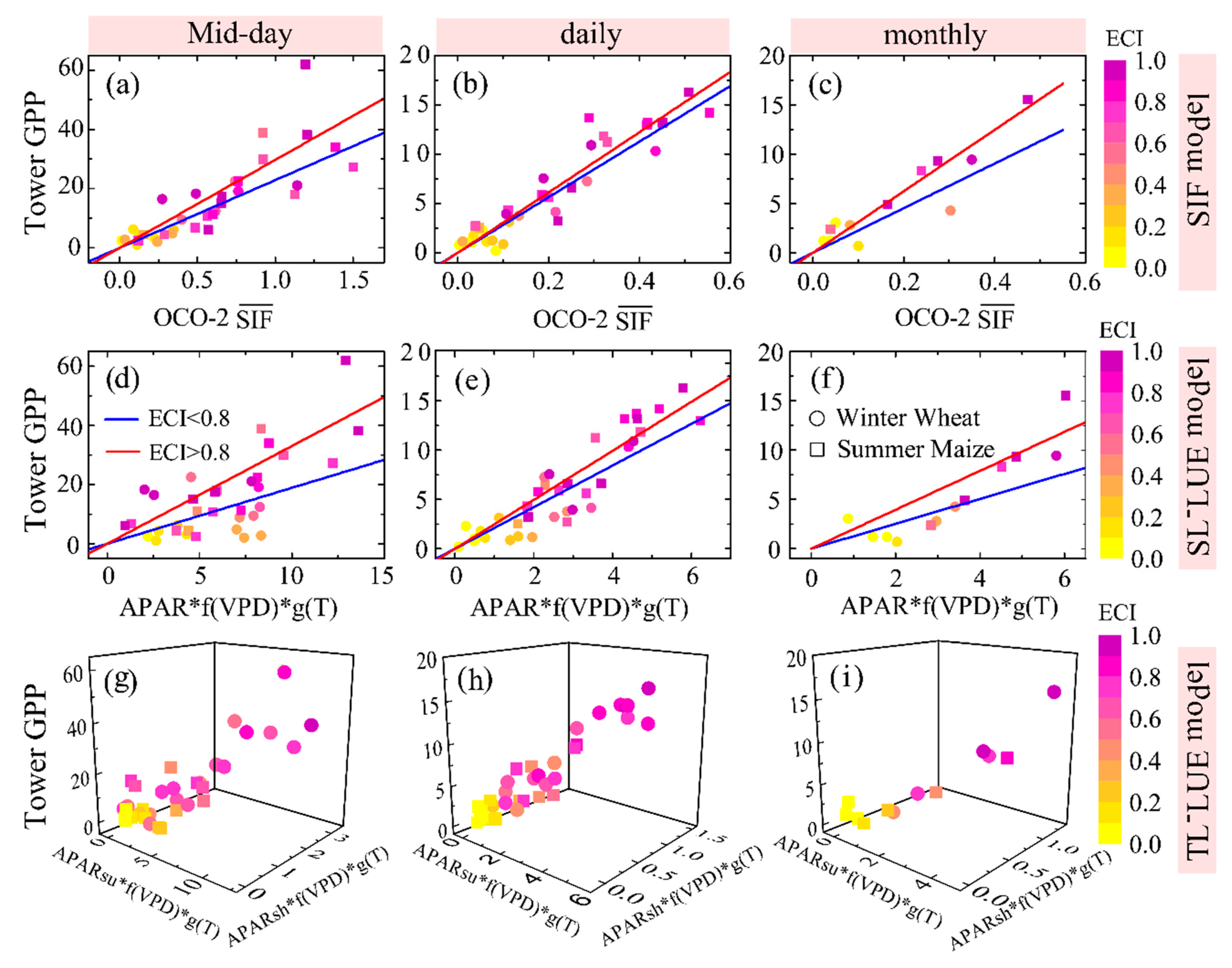
3.2. Comparison of Parameter Stability of the SIF and LUE Models across Multiple Temporal Aggregation Levels

We optimized the key parameters ($\epsilon /SI{F}_{\mathrm{yield}}$, ${\epsilon }_{\max }$, ${\epsilon }_{\mathrm{msu}}$, and ${\epsilon }_{\mathrm{msh}}$) of the SIF model, SL-LUE model, and TL-LUE model on mid-day, daily, and monthly timescales, respectively, to explore the stability of these parameters (Figure 3,

Table 2. The posterior estimations of $\epsilon /SI{F}_{yield}$ (gC m⁻² day⁻¹ (W m⁻² $\mathsf{\mu }$m⁻¹ sr⁻¹) ⁻¹) in the SIF model, ${\epsilon }_{\max }$ (gC MJ⁻¹) in the SL-LUE model, ${\epsilon }_{\mathrm{msu}}$ (gC MJ⁻¹) and ${\epsilon }_{\mathrm{msh}}$ (gC MJ⁻¹) in the TL-LUE model, and the coefficient of variation (CV, equal to 100% × standard deviation divided by the mean) of these optimizing parameters from mid-day to monthly timescales in 2015. All correlations were statistically significant (p < 0.001).

Models and Model Parameters		Mid-Day		Daily		Monthly		CV (%)
		Fitted Values	R2	Fitted Values	R2	Fitted Values	R2
OCO-2 SIF model	$\epsilon /SI{F}_{\mathrm{yield}}{}_{}$	26.31 (±3.89)	0.67	29.70 (±2.70)	0.83	28.43 (±2.60)	0.89	6.1
SL-LUE model	${\epsilon }_{\max }$	2.51 (±0.47)	0.51	2.33 (±0.21)	0.81	2.50 (±0.32)	0.80	4.1
TL-LUE model	${\epsilon }_{\mathrm{msu}}$	2.70 (±0.99)	0.70	2.15 (±0.51)	0.90	1.88 (±1.07)	0.93	18.6
	${\epsilon }_{\mathrm{msh}}$	4.30 (±3.95)		4.80 (±1.95)		8.58 (±4.96)		39.7

). In general, the goodness of fit in these three models was better on the daily and monthly timescales than on the mid-day timescale, which is consistent with the results reported by [37] and [1]. Across all temporal aggregation levels, the TL-LUE model was better than the SIF model and the SL-LUE model at capturing and explaining the seasonal fluctuations of GPP. The corresponding R² were 0.70, 0.90, and 0.93 for the mid-day, daily, and monthly timescales, respectively, slightly higher than those of the SIF model by 4.3%, 7.8%, and 4.3%, and much higher than those of the SL-LUE model by 27.1%, 10%, and 14.0%. However, it is noteworthy that the posterior estimations of $\epsilon /SI{F}_{\mathrm{yield}}$ in the SIF model and ${\epsilon }_{\max }$ in the SL-LUE model was relatively convergent across all temporal aggregation levels (Table 2). The CV of $\epsilon /SI{F}_{\mathrm{yield}}$ and ${\epsilon }_{\max }$ were 6.1% and 4.1%, which were on average 13.5% (±0.97%) and 34.3% (±1.28%) lower than those of ${\epsilon }_{\mathrm{msu}}$ and ${\epsilon }_{\mathrm{msh}}$. These analyses indicate the existence of both a robust GPP–SIF linear relationship and a good ability to capture seasonal variation in GPP across multiple temporal aggregation levels in the SIF-based model, compared with LUE-based models.

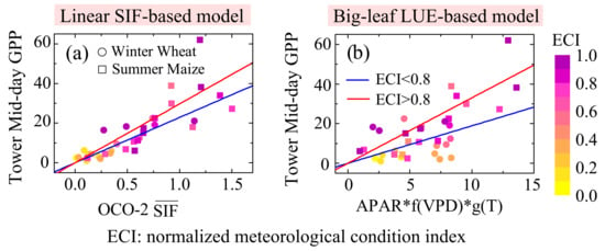
3.3. Comparison of Parameter Sensitivity of the SIF and LUE Models under Multiple Meteorological Conditions

The sensitivity of environmental factors in the SIF and LUE models was further independently analyzed at mid-day, daily, and monthly timescales. The ECI well summarized the information contained in the three environmental variables (APAR, air temperature, VPD) (Figure 4) and provided an objective and simple criterion to describe the extent of meteorological conditions experienced by the vegetation and photosynthetic devices. Across all temporal aggregations, we found that ECIs higher than 0.8 occurred in the later growth phase of wheat, the early growth stage of maize, and over the whole growth phase of summer maize from early July to early October (Figure 4). The high ECI values of wheat were mainly due to high air temperature and VPD, with high VPD occurring at the beginning of the growing phase of summer maize. This might be due to the lack of sprinkler irrigation during this period with high temperature, leading to higher VPD values, because the irrigation in the CN-YuC site is mainly used during the growth period of wheat. The high ECI values of the maize were mostly due to exposure to an environment with high light and high air temperature. This could be explained by the precipitation being concentrated between June and August, thus keeping sufficient water vapor content in the air. Therefore, the corresponding VPD values were lower even though the temperature was high during this period.

Figure 5 and

Table 3. The posterior estimations and the coefficients of variation (CV = standard deviations/mean × 100%) of $\epsilon /SI{F}_{\mathrm{yield}}$ (gC m⁻² day⁻¹ (W m⁻² $\mathsf{\mu }$m⁻¹ sr⁻¹) ⁻¹) in the SIF model, ${\epsilon }_{\max }$ (gC MJ⁻¹) in the SL-LUE model, and ${\epsilon }_{\mathrm{msu}}$ (gC MJ⁻¹) and ${\epsilon }_{\mathrm{msh}}$ (gC MJ⁻¹) in the TL-LUE model, with ECI values greater than 0.8 and less than 0.8 on the mid-day, daily, and monthly timescales, respectively. The “M” in gC MJ⁻¹ equals 10⁻⁶.

Time Scales	Parameters	ECI < 0.8	ECI > 0.8	CV (%)
mid-day	$\epsilon /SI{F}_{yield}$	23.09 (±4.67)	29.28 (±7.6)	16.7
	${\epsilon }_{\max }$	1.89 (±0.57)	3.30 (±0.74)	38.4
	${\epsilon }_{msu}$	1.05 (±1.04)	3.79 (±2.08)	80.0
	${\epsilon }_{msh}$	7.75 (±3.46)	1.23 (±10.60)	102.8
daily	$\epsilon /SI{F}_{yield}$	28.18 (±2.99)	30.56 (±3.92)	5.7
	${\epsilon }_{\max }$	2.11 (±0.34)	2.48 (±0.30)	11.5
	${\epsilon }_{msu}$	1.64 (±0.95)	2.28 (±0.73)	23.0
	${\epsilon }_{msh}$	5.70 (±3.22)	4.63 (±2.91)	14.7
monthly	$\epsilon /SI{F}_{yield}$	22.61 (±10.69)	31.16 (±5.04)	22.5
	${\epsilon }_{\max }$	1.26 (±0.49)	1.97 (±0.84)	31.0
	${\epsilon }_{msu}$	1.09 (±2.33)	0.75 (±0.88)	26.6
	${\epsilon }_{msh}$	5.11 (±10.68)	9.39 (±4.20)	41.8

further show the fluctuations of parameters in the SIF and LUE models under a range of different meteorological conditions using 0.8 as a threshold value of ECI values to fit separately. Overall, the relationship remained linear without significant nonlinearity, though there is one point at which large ECI values deviated from the linear relationship on the mid-day timescale (the left panel of Figure 5a,d), which agrees with the results reported by [3]. However, all curves showed a slight change in the direction of their slopes with different values of air temperature, APAR, and VPD at individual timescales. For all three models, we noted that the posterior estimations of their parameters had the smallest $CV$ values on the daily timescale, while larger fluctuations occurred on both the mid-day and monthly timescales. A detailed comparison is shown in Table 3. The values of $\epsilon /SI{F}_{yield}$ were relatively constant, with $CV$ values ranging from 5.7% at the daily timescale to 22.5% at the monthly timescale, about one-half of the ${\epsilon }_{\max }$ CVs and one-quarter of the ${\epsilon }_{\mathrm{msu}}$ and ${\epsilon }_{\mathrm{msh}}$ CVs. These results thus enhance the confidence of using SIF to simulate ecosystem-scale GPP under varying meteorological conditions.

3.4. Validation of LUE-Based and SIF-Based Models

The estimation performances of the LUE models and the linear SIF model were finally evaluated using the testing dataset from the year 2016 at the CN-YuC site. Maize photosynthesis started around mid-June with a rapid rise in GPP and ended in mid-October with GPP approaching zero, while wheat photosynthesis started around late February after the overwintering period and ended in mid-June. In general, GPP_SL-LUE, GPP_TL-LUE, and GPP_SIF captured the seasonal variations and magnitude of tower GPP well, except for some underestimation for the growth stage of maize on the mid-day timescale (Figure 6a). By contrast, the SIF model and the TL-LUE model could better describe the trajectory of the whole growing period of summer maize and winter wheat, and especially better described the fluctuation details for the early (“green-up”) and late (senescence) phases compared with SL-LUE (Figure 6a–c).

As a result, the SIF model and TL-LUE model had higher values of R² and lower values of RMSE than the SL-LUE model across all temporal aggregation levels (Figure 6;

Table 4. R², bias (observations minus simulations), root-mean-square error (RMSE), and relative/normalized RMSE (RRMSE) of the mid-day, daily, and monthly GPP (in gC m⁻² d⁻¹) in 2016 for the SIF model, SL-LUE model, and TL-LUE model, respectively. The units of bias and RMSE are both gC m⁻² d⁻¹. The unit of relative RMSE is %.

	Scale	Mid-Day					Daily				Monthly
Models		R2	RMSE	RRMSE	Bias	R2	RMSE	NRMSE	Bias	R2	RMSE	RRMSE	Bias
SIF model		0.59	9.23	15.61	0.55	0.77	2.50	13.49	0.84	0.94	0.59	4.06	0.98
SL-LUE		0.42	11.32	19.15	0.31	0.71	2.82	15.21	0.63	0.84	1.10	7.57	0.63
TL-LUE		0.68	9.03	15.28	0.50	0.83	2.51	13.54	0.75	0.98	0.65	4.47	0.91

), which is consistent with the fitted coefficient of determination using the training dataset in Table 2. The averaged changing trajectory of GPP explained by the SIF model and TL-LUE model was 77% and 83%, respectively. The averaged R² values were better than that of the SL-LUE model by 15.5% and 23.9%, and the corresponding average RRMSE values decreased by 2.9% and 2.9%, respectively (Table 4). Although the averaged biases of the SL-LUE model were lower than the biases of the SIF and TL-LUE models, its fluctuations in bias values were much greater. The small biases of the SL-LUE model might be due to bias items with opposite signs that cancel each other. Overall, the model performance in predicting GPP was ranked in three tiers as: TL-LUE > SIF model > SL-LUE. Moreover, the cross-validation and prediction results show that the SIF model and the TL-LUE model both have good stability and powerful prediction ability. These results indicate that the performance of the SIF models was comparable to the LUE models and actually better than the SL-LUE model, even though the SIF models were completely based on SIF and did not contain any ancillary data (e.g., temperature, radiation, VPD).

4. Discussion

4.1. Effects of Viewing Zenith Angle in OCO-2 Glint Mode

The robustness of the GPP–SIF relationships is affected by the quality of SIF retrievals, the accuracy of the carbon fluxes, as well as the homogeneity of the studied ecosystems. Because of OCO-2’s high discrete coverage, the SIF data in this study were obtained within a radius of 150 km centered at the flux tower to increase the number of soundings. Although only the SIF data with a cropland fraction greater than 80% were used to establish the SIF–GPP function (Table 1), this could also cause a footprint mismatch between the OCO-2 SIF and tower observations to some extent.

On the other hand, Sun et al. [11] has suggested that the effects of VZAs should be considered when using OCO-2 Glint or Target modes. We found that there is little difference between SIF values with and without VZA restriction except for two threshold values (Figure 1a), while the slope of the GPP–SIF relationship with VZA ranging between 20° and 40° exhibited slightly higher values than those with other VZAs (Figure 1b). The circumstances are not exactly the same as the directional effect on the SIF emission in Target mode that was reported by [1]. Li et al. [1] showed that the averaged SIF values and GPP–SIF relationship were almost unaffected when VZA was less than 40°, while the averaged SIF with VZA greater than 40° exhibited slightly higher values than those with all VZAs and the resulting GPP–SIF relationships were slightly different from those with smaller VZAs. This might be due to the VZA changes in different ways between the Target mode and Glint mode. In the Target mode, a great amount of measurements at different VZA values was acquired when the satellite focused on the ground sites during the overpass time. However, the viewing geometry of the Glint mode changed as the position of the land dark-spot varies over the season from east to west. That is, the average SIF with 20° < VZA ≤ 40° occurred in the growing season of winter wheat, while the SIF with 0° < VZA ≤ 20° appeared at the ripening stage of winter wheat and the early stage of summer maize, and the SIF with VZA > 40° appeared at the seedling stage of winter wheat. The corresponding SIF values with VZA ≤ 40° exhibited slightly higher values compared with those VZA > 40° (Figure 1a), and consequently, the GPP–SIF function had certain deviations with the SIF soundings with high VZA values (Figure 1b). The slope of the GPP–SIF is inconsistent between VZA ≤ 20° and 20° < VZA ≤ 40°, which had similar SIF values, which may be mainly because of the different cropland types (C3 winter wheat–fix and reduce inorganic CO₂ into organic compounds using only the C3 pathway in photosynthesis and C4 summer maize) in this study site. Therefore, the difference in the slopes of the GPP and SIF functions in this study may partly be attributable to the combining of the SIF Glint and Nadir mode observations and cropland types. There is still much to learn, and further validations with more flux sites are still needed to address the specific effects of VZAs in Glint mode on SIF values and on the relationship between SIF and GPP at different spatial scales and other ecosystems, as well as the mechanism between them.

4.2. Temporal Scaling Effect on the SIF-Based and LUE-Based Models

There was no evidence of obvious nonlinearity or changes in the slope ($\epsilon /SI{F}_{\mathrm{yield}}$) direction of the SIF-based model across the mid-day to monthly timescales (Figure 3; Table 2), which is consistent with previous results [13,37,66]. Guanter et al. [13] points out that the responses of GPP to light at the ecosystem-scale display low saturation levels when considering the mid-day (half-hourly) data and become further linearized with increasing spatial or temporal aggregation. Similar results were demonstrated in [37], and the GPP–SIF relationship remained consistent from mid-day to monthly timescales for both the maize and landscape ecosystem (

Table 5. The slope, R², and the coefficients of variation (CV = standard deviations/mean × 100%) of the linear GPP–SIF model in this study, from Wood et al. [37].

	Ecosystem	Time Scale	Slope	R2	CV of the Slope
This study	maize–wheat rotation	Mid-day	26.31 (±3.89)	0.67	6.1
		Daily	29.70 (±2.70)	0.83
		monthly	28.43 (±2.60)	0.89
Wood et al. [37]	Corn	Mid-day	23.2 (±2.8)	0.81	9.0
		Daily	19.9 (±0.88)	0.97
		monthly	23.5 (±1.15)	0.98
	Landscape	Mid-day	15.6 (±2.1)	0.79	5.8
		Daily	14.8 (±1.81)	0.82
		monthly	13.9 (±1.3)	0.92

). The linear correlation between GPP and SIF tends to converge across different timescales and may primarily depend on the fact that SIF is only emitted from photosystems and is closely linked to the fraction of PAR absorbed by the chlorophyll in all leaves of the canopy ($fPA{R}_{\mathrm{chl}}$) [38,67]. Zhang et al. [38] derived an estimation of the $fPA{R}_{\mathrm{chl}}$, which defined by $SIF/\cos \left(SZA\right)$ from 127 flux tower sites, and found that the light use efficiency ($\epsilon$) showed a spatial-temporal convergence using chlorophyll-absorbed light ($PA{R}_{\mathrm{chl}}$) to fix carbon dioxide. Moreover, both theoretical and experimental investigations have suggested that the two terms ($\epsilon$ and $SI{F}_{\mathrm{yield}}$) in the SIF model covary and the ratio of one to the other tends to be constant under high light intensities [67,68]. In this case, it is possible to conserve the GPP–SIF relationship across space and time.

By comparison, the values of the ${\epsilon }_{\max }$ in the SL-LUE model were similarly robust as $\epsilon /SI{F}_{yield}$ and considerably more stable than ${\epsilon }_{\mathrm{msu}}$ and ${\epsilon }_{\mathrm{msh}}$ in the TL-LUE for all temporal aggregation levels. As for the SL-LUE model, at the site scale, the photoresponse of an unstressed canopy is generally more linear for the variation in light absorption, along with canopy depth [69], and the slope of this photosynthesis–APAR relationship is the ${\epsilon }_{\max }$. The ${\epsilon }_{\max }$ value at the satellite overpass time (e.g., mid-day) is close to that of the daily average [70,71], and the relative similarity between the mid-day and daily ${\epsilon }_{\max }$ values also appears on the annual scale. As for the TL-LUE model, two possibilities exist for the large fluctuations of ${\epsilon }_{\mathrm{msu}}$ and ${\epsilon }_{\mathrm{msh}}$. First, the diffuse and direct radiation were partitioned using the exponential model with default parameters [72], which would result in uncertainty in the estimates of sunlit and shaded GPP. Additionally, it should be noted that any deviation of the parameter may also be related to biases in the GPP simulations [11]. The second possibility to consider is that no unique solution for ${\epsilon }_{\mathrm{msu}}$ and ${\epsilon }_{\mathrm{msh}}$ occurs at different spatial or temporal scales. The boundary conditions of ${\epsilon }_{\mathrm{msu}}$ and ${\epsilon }_{\mathrm{msh}}$ were set according to their observations and previous research results to separate their contribution, but lacked the specific constraint functions between them for the current study. Although previous studies (e.g., [5,28,31]) have shown that a linearly relationship exists between either ${\epsilon }_{\max }$ and ${\epsilon }_{\mathrm{msu}}$ or ${\epsilon }_{\max }$ and ${\epsilon }_{\mathrm{msh}}$ based on a number of statistical results, but is not clear yet, thus there is no unified equation of them in LUE models so far. These analyses suggest that the existence of both robust parameters and a good ability to capture seasonal variation in GPP may be in the SIF model, compared with the SL-LUE model, which has a robust argument, but poorer performance, and the TL-LUE model, which has unstable arguments, but better performance.

4.3. Environmental Restrictions on the SIF-Based and LUE-Based Models

The parameters of these three models all showed fluctuations to some extent under different ECI values of which contained the information of the air temperature, APAR, and VPD. However, the CV values of $\epsilon /SI{F}_{\mathrm{yield}}$ in the SIF model were relatively small under different ambient conditions in each independent temporal aggregation compared with those values in the SL-LUE and TL-LUE models (Figure 5; Table 3). It was also found by [3] that the GPP–SIF relationship in grassland tended to remain linear at the canopy scale with different meteorological conditions. Physiological stress caused by excessive light is known to affect the photochemical yield and fluorescence [73,74]. For the SIF model, the values of $\epsilon /SI{F}_{\mathrm{yield}}$ showed the greatest change with a CV of 16.7% and 22.5% at the mid-day and monthly timescales, which is possibly attributable to the dramatic changes in the slope as the ECI values change (Figure 7a,c). Moreover, at the mid-day and daily timescales, the linear relationship between $\epsilon$ and $SI{F}_{\mathrm{yield}}$ changed from a strong correlation (average R² value of 0.70) to a weak correlation (average R² value of 0.30) as the ECI values increased (Figure 7a,b). Therefore, the weakening of covariation between the $\epsilon$ and $SI{F}_{\mathrm{yield}}$ is likely the cause of the small fluctuations in the slope in the SIF model. Furthermore, fluorescence, photochemical quenching (PQ), and non-photochemical quenching (NPQ) are mutually exclusive and competing pathways. Changes in the efficiency of one affects the efficiency of the other two pathways [75]. The stress-induced closing down of photochemical traps in photosystem-II increases the fluorescence yield as the lifespan of an excited electron lengthens, while stress-induced opening up of extra NPQ pathways causes the fluorescence to decrease [76]. Nevertheless, both the shutdown of photosynthetic reaction centers and the opening of NPQ pathways cause the photochemical yield to drop. The influences of an increasing NPQ on $\epsilon$ and $SI{F}_{\mathrm{yield}}$ are not necessarily proportional [3]. That is, the nonlinear effects of NPQ on $\epsilon$ and $SI{F}_{\mathrm{yield}}$ are complex, which may also be a reason for the distinct response of these models to the different meteorological conditions.

Additionally, sunlit leaves receive both direct and diffuse radiation and should have higher temperatures than shaded leaves, resulting in greater temperature gradients between the surrounding air and sunlit leaves. A former study has suggested that the different temperatures of sunlit and shaded leaves should be considered in the parameter optimization procedure in the TL-LUE model [31]. Moreover, it is also noted that the differences in leaf temperature can also cause disparities in the VPD of sunlit and shaded leaves. In the LUE-based models, the application of the same VPD and air temperature scalars to the whole canopy may also be a source of uncertainty in the optimized parameters and estimated GPP [30]. Therefore, although we partitioned the efficiency ($\epsilon$) term of the LUE-based models into fixed parts (${\epsilon }_{\max }$, ${\epsilon }_{\mathrm{msu}}$, and ${\epsilon }_{\mathrm{msh}}$) that depict the optimal efficiency and variable components that represent the effects of light, temperature, and water stress (e.g., VPD), the sensitivity of the LUE models to the ECI may be the main cause of the larger fluctuations in the parameter values.

4.4. Estimation Performances of the SIF-Based and LUE-Based Models

The performances of the three GPP models were highly consistent in their predictions of the magnitudes and seasonal dynamics of GPP, as validated using GPP observations (Figure 6). The performance of the SIF model was better than that of the SL-LUE model and was only slightly poorer than that of the TL-LUE model. Similar to this study, previous research (see

Table 6. The estimation performance among different GPP models in this study, from Cui et al. [4] and Wagle et al. [44]. The unit of RMSE is gC m⁻² d⁻¹.

Ecosystem	Models		R2	RMSE
This study (maize–wheat rotation)	OCO-2 SIF model	Mid-day	0.59	9.23
		Daily	0.77	2.50
		monthly	0.94	0.59
	SL-LUE model	Mid-day	0.42	11.32
		Daily	0.71	2.82
		monthly	0.84	1.10
	TL-LUE model	Mid-day	0.68	9.03
		Daily	0.83	2.51
		monthly	0.98	0.65
Cui et al. [4] (Maize)	GPP–SIF760	Half-hour	0.62	20.74
	GPP–SIF686	Half-hour	0.46	31.10
	MuSyQ-GPP	Half-hour	0.70	21.60
	BEPS model	Half-hour	0.87	12.96
Wagle et al. [44] (Maize)	GOME-2 SIF model	8-day	0.87	2.72
	VPM model	8-day	0.91	2.27
	SCOPE model	8-day	0.95	1.58
	MOD17A2	8-day	0.47	5.30

) indicates that the models performed better at the daily timescale compared to the mid-day and half-hour timescales. Furthermore, the goodness of fit in the process-based two-leaf model provides the best simulation, and the GOME-2 SIF linear model is also better than the big-leaf LUE model used in the MOD17A2 product.

Wagle et al. [44] demonstrated that SIF is more relevant to the PAR absorbed by the photosynthetic parts of the maize canopy. That is, the components of PAR related with the SIF are mainly absorbed by vegetation chlorophyll, while the SL-LUE model in this study uses the PAR absorbed by the plant canopy ($fPA{R}_{\mathrm{canopy}}$) to estimate GPP. However, vegetation photosynthesis and chlorophyll fluorescence can only be driven by the PAR absorbed by photosynthetic parts, not by non-photosynthetic parts, such as branches, senescent foliage, and stems. This may be the reason that the SIF model has a better performance than the SL-LUE model. Nonetheless, previous studies have indicated that remote sensing SIF retrievals tend to represent the top layer of the vegetation canopy, which is primarily composed of sunlit leaves, thereby causing deviation between the SIF-based simulation and the tower observations [35,39]. Similar results were found when we analyzed the relationship between the SIF and LAI, the latter including the LAI of both sunlit and shaded leaves. The values of R² for the relationship between the SIF and the LAI of sunlit leaves were all greater than 0.85, while the values of R² ranged from 0.62 to 0.70 and from 0.53 to 0.65 for the relationships between SIF and the LAI of the whole canopy and between SIF and the LAI of shaded leaves across multiple temporal aggregation levels, respectively (Figure 8). Although the $fPA{R}_{\mathrm{canopy}}$ was also used in the TL-LUE model, it explicitly considers the difference in the LUE and APAR of sunlit and shaded leaves within the canopy. He et al. [28] illustrated that considering the entire canopy as a big extended leaf and ignoring the difference in the LUE and APAR of leaves can cause biased values of the simulated GPP. Consequently, the TL-LUE model can reduce the bias in GPP simulated by the SL-LUE model and the SIF model. On the other hand, the LUE-based models depend on a set of biome-specific parameters (${\epsilon }_{\max }$, ${\epsilon }_{\mathrm{msu}}$, and ${\epsilon }_{\mathrm{msh}}$) and also require different inputs, such as air temperature, PAR, and water or soil moisture scalars, while the SIF-based models are completely based on SIF information without requiring any other ancillary variables. In this case, using SIF to estimate GPP may save computational resources and reduce the uncertainty in GPP estimates across spatial and temporal scales compared with the LUE-based algorithm.

In summary, there is a compelling amount of data that supports the existence of a linear relationship between GPP and SIF for cropland that (1) is uniform for different temporal aggregation levels and under different meteorological conditions, and (2) contains adequate information for modeling ecosystem-level GPP. Additionally, whether our assessments are applicable to areas other than the cropland (maize–wheat rotation) used in this study is a problem that needs to be addressed in future research, and further studies are also needed to extend this analysis to other croplands, such as soybean, for cross-site comparisons.

4.5. Suggestions for Remote Sensing SIF Applications in LUE-Based Modeling

Previous studies have demonstrated that remotely sensed SIF retrievals can not only offer another approach to explore the seasonal variations in the photosynthesis, but can also restrict the parameters in process-based models to improve GPP simulations [77]. On the one hand, the Soil-Canopy Observation, Photosynthesis and Energy balance (SCOPE) model provides a theoretical method for modeling canopy SIF and photosynthesis by constraining the estimates of the maximum carboxylation rate (Vc_max) by coupling the soil-vegetation-atmosphere-transfer (SVAT) model with radiation transmission models [77]. On the other hand, the SCOPE model can also combine the SIF data derived from satellites to infer GPP from the land surface process model or carbon cycle data assimilation system [78,79]. In addition to the advantages of SIF in process-based models, it is also beneficial to the development of LUE-based models. Verma et al. [3] report that the correlation between the observed and simulated LUE is improved slightly when the normalized PRI and SIF yield are combined as predictive factors in the framework of multiple linear regression. Many studies have also shown that SIF comprises not just the light absorption information, but also the LUE information [36]. Moreover, we found that the values of $\epsilon /SI{F}_{\mathrm{yield}}$ and ${\epsilon }_{\max }$ tend to converge across time in this study, which may provide a basis for combining the satellite products of PRI and SIF to track ecosystem LUE. Additionally, remote sensing SIF retrievals tend to represent the top layer of the vegetation canopy, primarily composed of sunlit leaves [35,39], which may provide information for further studies to determine the contribution of the sunlit leaves and the structural sensitivity of SIF signals escaping the canopy to refine SIF-based models. We also can assume that SIF observations can be used to constrain the maximum rates of sunlit leaves in the two-leaf LUE model to improve the robustness of their estimates in future studies.

5. Conclusions

In this study, the effects of temporal aggregation and meteorological conditions on the parameter robustness of OCO-2 SIF-based and LUE-based GPP models, as well as the models’ estimation performances were examined and compared, respectively, at a maize–wheat rotation site in Yucheng, China. The main findings are as follows:

(1) The values of $\epsilon /SI{F}_{\mathrm{yield}}$ in the SIF model and those of ${\epsilon }_{\max }$ in the SL-LUE model are similarly robust and both are considerably more stable than those of ${\epsilon }_{\mathrm{msu}}$ and ${\epsilon }_{\mathrm{msh}}$ in the TL-LUE model across all temporal aggregation levels. Under different meteorological conditions, all the parameters show a certain degree of fluctuation and are most affected at the mid-day scale, followed by the monthly scale and finally at the daily scale overall. Nonetheless, the averaged coefficient of variation of the $\epsilon /SI{F}_{\mathrm{yield}}$ was relatively small and obviously lower than those of ${\epsilon }_{\max }$, ${\epsilon }_{\mathrm{msu}}$, and ${\epsilon }_{\mathrm{msh}}$. Therefore, compared with the LUE-based models, for different temporal aggregation levels and environmental restrictions in cropland, the SIF-based model is a good predictor of GPP and its parameter is more likely to converge. Moreover, the SIF models were completely based on SIF and did not contain any ancillary inputs, such as air temperature, PAR, and VPD. This study thus strongly supports the continuous effort to take advantage of SIF for improved monitoring of GPP.

(2) It is feasible to combine the OCO-2 SIF data of the Nadir observation mode with those of the Glint observation mode after fully considering the viewing zenith effects of the latter on the magnitude of SIF values and on the relationship between SIF and GPP. This enables the limitation of sparse data to be alleviated and better exploration of the link between the ground-observed GPP and remote-sensing-based SIF retrievals at the canopy scale to be achieved. Additionally, the OCO-2 SIF data are found to be more strongly correlated with the LAI of sunlit leaves. It indicates that SIF observations may be useful to constrain the maximum photosynthetic rates of sunlit leaves in the two-leaf LUE model, thus reducing the uncertainty of parameter estimates and improving the accuracy of GPP prediction in future studies.

References

1. Li, X.; Xiao, J.; He, B. Chlorophyll fluorescence observed by OCO-2 is strongly related to gross primary productivity estimated from flux towers in temperate forests. Remote Sens. Environ. 2018, 204, 659–671. [Google Scholar] [CrossRef]
2. Odum, E.P.; Barrett, G.W.; Lu, J.J. Fundamentals of Ecology; Saunders: Philadelphia, PA, USA, 1971; Volume 5, pp. 87–88. [Google Scholar]
3. Verma, M.; Schimel, D.; Evans, B.; Frankenberg, C.; Beringer, J.; Drewry, D.T.; Magney, T.; Marang, I.; Hutley, L.; Moore, C.; et al. Effect of meteorological conditions on the relationship between solar-induced fluorescence and gross primary productivity at an OzFlux grassland site. J. Geophys. Res. Biogeosci. 2017, 122, 716–733. [Google Scholar] [CrossRef]
4. Cui, T.; Sun, R.; Qiao, C.; Zhang, Q.; Yu, T.; Liu, G.; Liu, Z. Estimating Diurnal Courses of Gross Primary Production for Maize: A Comparison of Sun-Induced Chlorophyll Fluorescence, Light-Use Efficiency and Process-Based Models. Remote Sens. 2017, 9, 1267. [Google Scholar] [CrossRef]
5. Lin, X.; Chen, B.; Chen, J.; Zhang, H.; Sun, S.; Xu, G.; Guo, L.; Ge, M.; Qu, J.; Li, L.; et al. Seasonal fluctuations of photosynthetic parameters for light use efficiency models and the impacts on gross primary production estimation. Agric. For. Meteorol. 2017, 236, 22–35. [Google Scholar] [CrossRef] [Green Version]
6. Zhang, Y.; Xiao, X.; Jin, C.; Dong, J.; Zhou, S.; Wagle, P.; Joiner, J.; Guanter, L.; Zhang, Y.; Zhang, G.; et al. Consistency between sun-induced chlorophyll fluorescence and gross primary production of vegetation in North America. Remote Sens. Environ. 2016, 183, 154–169. [Google Scholar] [CrossRef] [Green Version]
7. Frankenberg, C.; Fisher, J.B.; Worden, J.; Badgley, G.; Saatchi, S.S.; Lee, J.E.; Toon, G.C.; Butz, A.; Jung, M.; Kuze, A. New global observations of the terrestrial carbon cycle from GOSAT: Patterns of plant fluorescence with gross primary productivity. Geophys. Res. Lett. 2011, 38, L17706. [Google Scholar] [CrossRef]
8. Frankenberg, C.; O’Dell, C.; Berry, J.; Guanter, L.; Joiner, J.; Köhler, P.; Pollock, R.; Taylor, T.E. Prospects for chlorophyll fluorescence remote sensing from the orbiting carbon observatory-2. Remote Sens. Environ. 2014, 147, 1–12. [Google Scholar] [CrossRef]
9. Köhler, P.; Guanter, L.; Joiner, J. A linear method for the retrieval of sun-induced chlorophyll fluorescence from GOME-2 and SCIAMACHY data. Atmos. Meas. Tech. 2015, 8, 2589–2608. [Google Scholar] [CrossRef] [Green Version]
10. Sun, Y.; Frankenberg, C.; Wood, J.D.; Schimel, D.S.; Jung, M.; Guanter, L.; Drewry, D.T.; Verma, M.; Porcar-Castell, A.; Griffis, T.J.; et al. OCO-2 advances photosynthesis observation from space via solar-induced chlorophyll fluorescence. Science 2017, 358, eaam5747. [Google Scholar] [CrossRef] [Green Version]
11. Sun, Y.; Frankenberg, C.; Jung, M.; Joiner, J.; Guanter, L.; Köhler, P.; Magney, T. Overview of Solar-Induced chlorophyll Fluorescence (SIF) from the Orbiting Carbon Observatory-2: Retrieval, cross-mission comparison, and global monitoring for GPP. Remote Sens. Environ. 2018, 209, 808–823. [Google Scholar] [CrossRef]
12. Joiner, J.; Yoshida, Y.; Vasilkov, A.P.; Middleton, E.M. First observations of global and seasonal terrestrial chlorophyll fluorescence from space. Biogeosciences 2011, 8, 637–651. [Google Scholar] [CrossRef] [Green Version]
13. Guanter, L.; Frankenberg, C.; Dudhia, A.; Lewis, P.E.; Gómez-Dans, J.; Kuze, A.; Suto, H.; Grainger, R.G. Retrieval and global assessment of terrestrial chlorophyll fluorescence from GOSAT space measurements. Remote Sens. Environ. 2012, 121, 236–251. [Google Scholar] [CrossRef]
14. Joiner, J.; Yoshida, Y.; Vasilkov, A.P.; Middleton, E.M.; Campbell, P.K.E.; Kuze, A. Filling-in of near-infrared solar lines by terrestrial fluorescence and other geophysical effects: Simulations and space-based observations from SCIAMACHY and GOSAT. Atmos. Meas. Tech. 2012, 5, 809–829. [Google Scholar] [CrossRef]
15. Joiner, J.; Guanter, L.; Lindstrot, R.; Voigt, M.; Vasilkov, A.P.; Middleton, E.M.; Huemmrich, K.F.; Yoshida, Y.; Frankenberg, C. Global monitoring of terrestrial chlorophyll fluorescence from moderate-spectral-resolution near-infrared satellite measurements: Methodology, simulations, and application to GOME-2. Atmos. Meas. Tech. 2013, 6, 2803–2823. [Google Scholar] [CrossRef]
16. Sanders, A.; Verstraeten, W.; Kooreman, M.; Van Leth, T.; Beringer, J.; Joiner, J. Spaceborne sun-induced vegetation fluorescence time series from 2007 to 2015 evaluated with Australian flux tower measurements. Remote Sens. 2016, 8, 895. [Google Scholar] [CrossRef]
17. Joiner, J.; Yoshida, Y.; Guanter, L.; Middleton, E.M. New methods for the retrieval of chlorophyll red fluorescence from hyperspectral satellite instruments: Simulations and application to GOME-2 and SCIAMACHY. Atmos. Meas. Tech. 2016, 9, 3939–3967. [Google Scholar] [CrossRef]
18. Wolanin, A.; Rozanov, V.V.; Dinter, T.; Noël, S.; Vountas, M.; Burrows, J.P.; Bracher, A. Global retrieval of marine and terrestrial chlorophyll fluorescence at its red peak using hyperspectral top of atmosphere radiance measurements: Feasibility study and first results. Remote Sens. Environ. 2015, 166, 243–261. [Google Scholar] [CrossRef] [Green Version]
19. Jeong, S.J.; Schimel, D.; Frankenberg, C.; Drewry, D.T.; Fisher, J.B.; Verma, M.; Berry, J.A.; Lee, J.E.; Joiner, J. Application of satellite solar-induced chlorophyll fluorescence to understanding large-scale variations in vegetation phenology and function over northern high latitude forests. Remote Sens. Environ. 2017, 190, 178–187. [Google Scholar] [CrossRef]
20. Luus, K.A.; Commane, R.; Parazoo, N.C.; Benmergui, J.; Euskirchen, E.S.; Frankenberg, C.; Joiner, J.; Lindaas, J.; Miller, C.E.; Oechel, W.C.; et al. Tundra photosynthesis captured by satellite-observed solar-induced chlorophyll fluorescence. Geophys. Res. Lett. 2017, 44, 1564–1573. [Google Scholar] [CrossRef]
21. Guanter, L.; Zhang, Y.; Jung, M.; Joiner, J.; Voigt, M.; Berry, J.A.; Frankenberg, C.; Huete, A.R.; Zarco-Tejada, P.; Lee, J.E.; et al. Global and time-resolved monitoring of crop photosynthesis with chlorophyll fluorescence. Proc. Natl. Acad. Sci. USA 2014, 111, E1327–E1333. [Google Scholar] [CrossRef] [Green Version]
22. Guan, K.; Berry, J.A.; Zhang, Y.; Joiner, J.; Guanter, L.; Badgley, G.; Lobell, D.B. Improving the monitoring of crop productivity using spaceborne solar-induced fluorescence. Glob. Chang. Biol. 2016, 22, 716–726. [Google Scholar] [CrossRef] [PubMed]
23. Lee, J.E.; Frankenberg, C.; van der Tol, C.; Berry, J.A.; Guanter, L.; Boyce, C.K.; Fisher, J.B.; Morrow, E.; Worden, J.R.; Asefi, S. Forest productivity and water stress in Amazonia: Observations from GOSAT chlorophyll fluorescence. Proc. R. Soc. B Biol. Sci. 2013, 280, 20130171. [Google Scholar] [CrossRef] [PubMed]
24. Guan, K.; Pan, M.; Li, H.; Wolf, A.; Wu, J.; Medvigy, D.; Caylor, K.K.; Sheffield, J.; Wood, E.F.; Malhi, Y.; et al. Photosynthetic seasonality of global tropical forests constrained by hydroclimate. Nat. Geosci. 2015, 8, 284. [Google Scholar] [CrossRef]
25. Wang, J.B.; Dong, J.W.; Liu, J.Y.; Huang, M.; Li, G.C.; Running, S.W.; Smith, W.K.; Harris, W.; Saigusa, N.; Kondo, H. Comparison of gross primary productivity derived from GIMMS NDVI3g, GIMMS, andMODIS in Southeast Asia. Remote Sens. 2014, 6, 2108–2133. [Google Scholar] [CrossRef]
26. Hongji, Z.; Aiwen, L.; Lunche, W.; Yu, X.; Ling, Z. Evaluation of modis gross primary production across multiple biomes in china using eddy covariance flux data. Remote Sens. 2016, 8, 395. [Google Scholar] [CrossRef]
27. Lunche, W.; Hongji, Z.; Aiwen, L.; Ling, Z.; Wenmin, Q.; Qiyong, D. Evaluation of the latest modis gpp products across multiple biomes using global eddy covariance flux data. Remote Sens. 2017, 9, 418. [Google Scholar] [CrossRef]
28. He, M.; Ju, W.; Zhou, Y.; Chen, J.; He, H.; Wang, S.; Wang, H.; Guan, D.; Yan, J.; Li, Y.; et al. Development of a two-leaf light use efficiency model for improving the calculation of terrestrial gross primary productivity. Agric. For. Meteorol. 2013, 173, 28–39. [Google Scholar] [CrossRef]
29. Schaefer, K.; Schwalm, C.R.; Williams, C.; Arain, M.A.; Barr, A.; Chen, J.M.; Davis, K.J.; Dimitrov, D.; Hilton, T.W.; Hollinger, D.Y. A model-data comparison of gross primary productivity: Results from the North American Carbon Program site synthesis. J. Geophys. Res. Biogeosci. 2012, 117, G03010. [Google Scholar] [CrossRef]
30. Zhou, Y.; Wu, X.; Ju, W.; Chen, J.M.; Wang, S.; Wang, H.; Yuan, W.; Black, T.A.; Jassal, R.; Ibrom, A.; et al. Global parameterization and validation of a two-leaf light use efficiency model for predicting gross primary production across FLUXNET sites. J. Geophys. Res. Biogeosci. 2016, 121, 1045–1072. [Google Scholar] [CrossRef]
31. Li, A.; Bian, J.; Lei, G.; Huang, C. Estimating the maximal light use efficiency for different vegetation through the CASA Model combined with time-series remote sensing data and ground measurements. Remote Sens. 2012, 4, 3857–3876. [Google Scholar] [CrossRef]
32. Chen, J.; Zhang, H.; Liu, Z.; Che, M.; Chen, B. Evaluating Parameter Adjustment in the MODIS Gross Primary Production Algorithm Based on Eddy Covariance Tower Measurements. Remote Sens. 2014, 6, 3321–3348. [Google Scholar] [CrossRef] [Green Version]
33. Baldocchi, D.D. Must we incorporate soil moisture information when applying light use efficiency models with satellite remote sensing information? New Phytol. 2018, 218, 1293–1294. [Google Scholar] [CrossRef] [PubMed] [Green Version]
34. Muramatsu, K.; Furumi, S.; Soyama, N.; Daigo, M. Estimating the seasonal maximum light use efficiency. In Proceedings of the SPIE Asia-Pacific Remote Sensing, Beijing, China, 8 November 2014. [Google Scholar]
35. Damm, A.; Guanter, L.; Paul-Limoges, E.; Van der Tol, C.; Hueni, A.; Buchmann, N.; Eugster, W.; Ammann, C.; Schaepman, M.E. Far-red sun-induced chlorophyll fluorescence shows ecosystem-specific relationships to gross primary production: An assessment based on observational and modeling approaches. Remote Sens. Environ. 2015, 166, 91–105. [Google Scholar] [CrossRef]
36. Yang, H.; Yang, X.; Zhang, Y.; Heskel, M.A.; Lu, X.; Munger, J.W.; Sun, S.; Tang, J. Chlorophyll fluorescence tracks seasonal variations of photosynthesis from leaf to canopy in a temperate forest. Glob. Chang. Biol. 2017, 23, 2874–2886. [Google Scholar] [CrossRef] [PubMed]
37. Wood, J.D.; Griffis, T.J.; Baker, J.M.; Frankenberg, C.; Verma, M.; Yuen, K. Multiscale analyses of solar-induced florescence and gross primary production. Geophys. Res. Lett. 2017, 44, 533–541. [Google Scholar] [CrossRef]
38. Zhang, Y.; Xiao, X.; Wolf, S.; Wu, J.; Wu, X.; Gioli, B.; Wohlfahrt, G.; Cescatti, A.; van der Tol, C.; Zhou, S.; et al. Spatio-Temporal Convergence of Maximum Daily Light-Use Efficiency Based on Radiation Absorption by Canopy Chlorophyll. Geophys. Res. Lett. 2018, 45, 3508–3519. [Google Scholar] [CrossRef]
39. Bonan, G.B.; Lawrence, P.J.; Oleson, K.W.; Levis, S.; Jung, M.; Reichstein, M.; Lawrence, D.M.; Swenson, S.C. Improving canopy processes in the Community Land Model version 4 (CLM4) using global flux fields empirically inferred from fluxnet data. J. Geophys. Res. Biogeosci. 2011, 116, G02014. [Google Scholar] [CrossRef]
40. Chen, H.; Dickinson, R.E.; Dai, Y.; Zhou, L. Sensitivity of simulated terrestrial carbon assimilation and canopy transpiration to different stomatal conductance and carbon assimilation schemes. Clim. Dyn. 2010, 36, 1037–1054. [Google Scholar] [CrossRef]
41. Gamon, J.A. Reviews and syntheses: Optical sampling of the flux tower footprint. Biogeosciences 2015, 12, 4509–4523. [Google Scholar] [CrossRef]
42. Jia, W.; Liu, M.; Wang, D.; He, H.; Shi, P.; Li, Y.; Wang, Y. Uncertainty in simulating regional gross primary productivity from satellite-based models over northern China grassland. Ecol. Indic. 2018, 88, 134–143. [Google Scholar] [CrossRef]
43. Gamon, J.A.; Cheng, Y.; Claudio, H.; Mackinney, L.; Sims, D.A. A mobile tram system for systematic sampling of ecosystem optical properties. Remote Sens. Environ. 2006, 103, 246–254. [Google Scholar] [CrossRef]
44. Wagle, P.; Zhang, Y.; Jin, C.; Xiao, X. Comparison of solar-induced chlorophyll fluorescence, light-use efficiency, and process-based GPP models in maize. Ecol. Appl. 2016, 26, 1211–1222. [Google Scholar] [CrossRef] [PubMed]
45. Hilker, T.; Coops, N.C.; Nesic, Z.; Wulder, M.A.; Black, A.T. Instrumentation and approach for unattended year round tower based measurements of spectral reflectance. Comput. Electron. Agric. 2007, 56, 72–84. [Google Scholar] [CrossRef]
46. Wanner, W.; Li, X.; Strahler, A.H. On the derivation of kernels for kernel driven models of bidirectional reflectance. J. Geophys. Res. 1995, 100, 21077–21089. [Google Scholar] [CrossRef]
47. Lucht, W.; Schaaf, C.B.; Strahler, A.H. An algorithm for the retrieval of albedo from space using semiempirical BRDF models. IEEE Trans. Geosci. Remote Sens. 2000, 38, 977–998. [Google Scholar] [CrossRef] [Green Version]
48. Maier, S.W.; Günther, K.P.; Stellmes, M. Sun-induced fluorescence: A new tool for precision farming. In Digital Imaging and Spectral Techniques: Applications to Precision Agriculture and Crop Physiology; The American Society of Agronomy: Madison, WI, USA, 2003; pp. 209–222. [Google Scholar]
49. Wang, R.; Liu, Z.G.; Feng, H.K.; Yang, P.Q.; Wang, Q.S. Extraction and analysis of Solar—induced chlorophyl fluorescence of wheat with ground-based hyperspectral imaging system. Spectrosc. Spectr. Anal. 2013, 33, 2451–2454. [Google Scholar] [CrossRef]
50. Plascyk, J.A. The MK II Fraunhofer Line Discriminator (FLD-II) for Airborne and Orbital Remote Sensing of Solar-Stimulated Luminescence. Opt. Eng. 1975, 14, 339–346. [Google Scholar] [CrossRef]
51. Alonso, L.; Gomez-Chova, L.; Vila-Frances, J.; Amoros-Lopez, J.; Guanter, L.; Calpe, J.; Moreno, J. Improved Fraunhofer Line Discrimination Method for Vegetation Fluorescence Quantification. IEEE Geosci. Remote Sens. Lett. 2008, 5, 620–624. [Google Scholar] [CrossRef]
52. Damm, A.; Erler, A.; Hillen, W.; Meroni, M.; Schaepman, M.E.; Verhoef, W.; Rascher, U. Modeling the impact of spectral sensor configurations on the FLD retrieval accuracy of sun-induced chlorophyll fluorescence. Remote Sens. Environ. 2011, 115, 1882–1892. [Google Scholar] [CrossRef]
53. Liu, X.; Liu, L. Assessing band sensitivity to atmospheric radiation transfer for space-based retrieval of solar-induced chlorophyll fluorescence. Remote Sens. 2014, 6, 10656–10675. [Google Scholar] [CrossRef]
54. Liu, X.; Liu, L.; Zhang, S.; Zhou, X. New spectral fitting method for full-spectrum solar-induced chlorophyll fluorescence retrieval based on principal components analysis. Remote Sens. 2015, 7, 10626–10645. [Google Scholar] [CrossRef]
55. Liu, L.; Guan, L.; Liu, X. Directly estimating diurnal changes in GPP for C3 and C4 crops using far-red sun-induced chlorophyll fluorescence. Agric. For. Meteorol. 2017, 232, 1–9. [Google Scholar] [CrossRef]
56. Carlson, T.N.; Ripley, D.A. On the relation between NDVI, fractional vegetation cover, and leaf area index. Remote Sens. Environ. 1997, 62, 241–252. [Google Scholar] [CrossRef]
57. Vogelmann, J.E.; Rock, B.N.; Moss, D.M. Red edge spectral measurements from sugar maple leaves. Int. J. Remote Sens. 1993, 14, 1563–1575. [Google Scholar] [CrossRef]
58. Chen, M.; Deng, F.; Chen, M. Locally adjusted cubic-spline capping for reconstructing seasonal trajectories of a satellite-derived surface parameter. IEEE Trans. Geosci. Remote 2006, 44, 2230–2238. [Google Scholar] [CrossRef]
59. Monteith, J.L. Solar radiation and productivity in tropical ecosystems. J. Appl. Ecol. 1972, 9, 747–766. [Google Scholar] [CrossRef]
60. Fournier, A.; Daumard, F.; Champagne, S.; Ounis, A.; Goulas, Y.; Moya, I. Effect of canopy structure on sun-induced chlorophyll fluorescence. ISPRS J. Photogramm. Remote Sens. 2012, 68, 112–120. [Google Scholar] [CrossRef]
61. Chen, J.M.; Liu, J.; Cihlar, J.; Goulden, M.L. Daily canopy photosynthesis model through temporal and spatial scaling for remote sensing applications. Ecol. Model. 1999, 124, 99–119. [Google Scholar] [CrossRef] [Green Version]
62. Tang, S.; Chen, J.M.; Zhu, Q.; Li, X.; Chen, M.; Sun, R.; Zhou, Y.; Deng, F.; Xie, D. LAI inversion algorithm based on directional reflectance kernels. J. Environ. Manag. 2007, 85, 638–648. [Google Scholar] [CrossRef]
63. Bonett, D.G. Confidence interval for a coefficient of quartile variation. Comput. Stat. Data Anal. 2006, 50, 2953–2957. [Google Scholar] [CrossRef]
64. Willmott, C.J.; Ackleson, S.G.; Davis, R.E.; Feddema, J.J.; Klink, K.M.; Legates, D.R.; Donnell, J.O.; Rowe, C.M. Statistics for the evaluation and comparison of models. J. Geophys. Res. Atmos. 1985, 90, 8995–9005. [Google Scholar] [CrossRef] [Green Version]
65. Willmott, C.J.; Matsuura, K. Advantages of the mean absolute error (mae) over the root mean square error (rmse) in assessing average model performance. Clim. Res. 2005, 30, 79–82. [Google Scholar] [CrossRef]
66. Yang, X.; Tang, J.; Mustard, J.F.; Lee, J.E.; Rossini, M.; Joiner, J.; Munger, J.W.; Kornfeld, A.; Richardson, A.D. Solar-induced chlorophyll fluorescence that correlates with canopy photosynthesis on diurnal and seasonal scales in a temperate deciduous forest. Geophys. Res. Lett. 2015, 42, 2977–2987. [Google Scholar] [CrossRef]
67. Lee, J.E.; Berry, J.A.; van der Tol, C.; Yang, X.; Guanter, L.; Damm, A.; Baker, I.; Frankenberg, C. Simulations of chlorophyll fluorescence incorporated into the C ommunity L and M odel version 4. Glob. Chang. Biol. 2015, 21, 3469–3477. [Google Scholar] [CrossRef] [PubMed]
68. Joiner, J.; Yoshida, Y.; Vasilkov, A.P.; Schaefer, K.; Jung, M.; Guanter, L.; Zhang, Y.; Garrity, S.; Middleton, E.M.; Huemmrich, K.F.; et al. The seasonal cycle of satellite chlorophyll fluorescence observations and its relationship to vegetation phenology and ecosystem atmosphere carbon exchange. Remote Sens. Environ. 2014, 152, 375–391. [Google Scholar] [CrossRef] [Green Version]
69. Norman, J.M.; Arkebauer, T.J. Predicting canopy light-use efficiency from leaf characteristics. In Modeling Plant and Soil Systems; The American Society of Agronomy: Madison, WI, USA, 1991; pp. 125–143. [Google Scholar]
70. Goerner, A.; Reichstein, M.; Rambal, S. Tracking seasonal drought effects on ecosystem light use efficiency with satellite-based PRI in a Mediterranean forest. Remote Sens. Environ. 2009, 113, 1101–1111. [Google Scholar] [CrossRef]
71. Drolet, G.G.; Middleton, E.M.; Huemmrich, K.F.; Hall, F.G.; Amiro, B.D.; Barr, A.G.; Black, T.A.; McCaughey, J.H.; Margolis, H.A. Regional mapping of gross light-use efficiency using MODIS spectral indices. Remote Sens. Environ. 2008, 112, 3064–3078. [Google Scholar] [CrossRef]
72. Boland, J.; Ridley, B. Models of Diffuse Solar Fraction. In Modeling Solar Radiation at the Earth’s Surface; Springer: Berlin/Heidelberg, Germany, 2008; pp. 193–219. [Google Scholar]
73. Schreiber, U.; Hormann, H.; Neubauer, C.; Klughammer, C. Assessment of photosystem II photochemical quantum yield by chlorophyll fluorescence quenching analysis. Funct. Plant Biol. 1995, 22, 209–220. [Google Scholar] [CrossRef]
74. Weis, E.; Berry, J.A. Quantum efficiency of photosystem II in relation to ‘energy’-dependent quenching of chlorophyll fluorescence. BBA Bioenerg. 1987, 894, 198–208. [Google Scholar] [CrossRef]
75. Maxwell, K.; Johnson, G.N. Chlorophyll fluorescence—A practical guide. J. Exp. Bot. 2000, 51, 659–668. [Google Scholar] [CrossRef]
76. Mohammed, G.H.; Goulas, Y.; Magnani, F.; Moreno, J.; Olejníčková, J.; Rascher, U.; van der Tol, C.; Verhoef, W.; Ač, A.; Daumard, F.; et al. 2012 FLEX/Sentinel-3 Tandem Mission Photosynthesis Study; Final Report. ESTEC contract no. 4000106396/12/NL/AF; P & M Technologies: Sault Ste. Marie, ON, Canada, 2014. [Google Scholar]
77. Zhang, Y.; Guanter, L.; Berry, J.A.; van der Tol, C.; Joiner, J. Can we retrieve vegetation photosynthetic capacity paramter from solar-induced fluorescence? In Proceedings of the 2016 IEEE International Geoscience and Remote Sensing Symposium (IGARSS), Beijing, China, 10–15 July 2016; pp. 1711–1713. [Google Scholar] [CrossRef]
78. Koffi, E.N.; Rayner, P.J.; Norton, A.J.; Frankenberg, C.; Scholze, M. Investigating the usefulness of satellite-derived fluorescence data in inferring gross primary productivity within the carbon cycle data assimilation system. Biogeosciences 2015, 12, 4067–4084. [Google Scholar] [CrossRef] [Green Version]
79. MacBean, N.; Maignan, F.; Bacour, C.; Lewis, P.; Peylin, P.; Guanter, L.; Köhler, P.; Gómez-Dans, J.; Disney, M. Strong constraint on modelled global carbon uptake using solar-induced chlorophyll fluorescence data. Sci. Rep. 2018, 8, 1973. [Google Scholar] [CrossRef] [PubMed]
Figure 1. Effects of varying view zenith angle (VZA) on OCO-2 Glint SIF observations and the gross primary production (GPP)–SIF correlation at the mid-day timescale: (a) the differences between SIF with and without VZA restrictions: VZA ≤ 20 ; 20 < VZA ≤ 40 ; and VZA > 40 ; (b) the relationships of ground GPP and SIF under various intervals of VZAs: VZA ≤ 20 ; 20 < VZA ≤ 40 ; VZA > 40 ; and no restriction ( 0 < VZA ≤ 50 ). The data points are averages of the sounding for each point in the time referring to Table 1 and the error bar represents ±1 σ statistical uncertainty estimations of OCO-2 SIF.
Remotesensing 11 01328 g001
Figure 2. The consistency of OCO-2 SIF in Glint and Nadir observation modes with the tower derived SIF: (a) Seasonal dynamics of tower gross primary production (GPP), normalized difference vegetation index (NDVIBRDF), Vogelmann red edge index (VOGBRDF), tower sun-induced chlorophyll inflorescence (SIF), and OCO-2 SIF; (b) the relationship between OCO-2 SIF in Glint and Nadir modes and the tower SIF at the CN-YuC site over the 2015 growth period of summer maize. There are only six data points on Glint mode and seven data points on Nadir mode for both satellite overpassing and tower observing at the same time. The missing observations from 17 August 2015 to 1 September 2015 were due to an equipment failure.
Remotesensing 11 01328 g002
Figure 3. Fitting results of parameters for different models on different timescales in 2015. The columns from left to right show the mid-day, daily, and monthly timescales, respectively. The rows from top to bottom indicate the SIF model ( G P P ε / S I F yield × S I F ), the one-leaf light-use efficiency (SL-LUE) model ( G P P = ε max × A P A R × f ( V P D ) × g ( T a ) ), and the two-leaf LUE (TL-LUE) model ( G P P = ε msu × A P A R su × f ( V P D ) × g ( T a ) + ε msh × A P A R sh × f ( V P D ) × g ( T a ) ), respectively. There are 39 data points for mid-day and daily time scales and 12 data points for monthly time scale. The unit of tower GPP is gC m−2 day−1, the unit of OCO-2 SIF is W m−2 μ m−1 sr−1, and the unit of APAR × f(VPD) × g(T) is MJ m−2 day−1 (1 MJ = 106 J).
Remotesensing 11 01328 g003
Figure 4. Seasonal dynamics of normalized meteorological conditions (scaled within 0–1), including normalized meteorological condition index (ECI), air temperature, VPD, and APAR at the (a) mid-day timescale, (b) daily timescale, and (c) monthly timescale. The solid grey lines refer to the threshold value of ECI values. The whole canopies are prone to experiencing exposure to excess light when the ECI is greater than 0.8 compared with when the ECI is lower.
Remotesensing 11 01328 g004
Figure 5. The fluctuations in the parameters of the SIF model and the LUE models for a range of meteorological conditions, where 0.8 is the threshold value at which ECI values are fitted separately. The columns from left to right show the mid-day, daily, and monthly timescales, respectively. The rows from top to bottom indicate the SIF model ( G P P ε / S I F yield × S I F ), SL-LUE model ( G P P = ε max × A P A R × f ( V P D ) × g ( T a ) ), and TL-LUE model ( G P P = ε msu × A P A R su × f ( V P D ) × g ( T a ) + ε msh × A P A R sh × f ( V P D ) × g ( T a ) ), respectively. The unit of tower GPP is gC m−2 day−1, the unit of OCO-2 SIF is W m−2 μ m−1 sr−1, and the unit of APAR × f(VPD) × g(T) is MJ m−2 day−1 (1 MJ = 106 J).
Remotesensing 11 01328 g005
Figure 6. Validation of the SIF model, the SL-LUE model, and the TL-LUE model on the mid-day, daily, and monthly timescales in 2016, respectively. The panels (ac): the seasonal variations of simulated and tower observed GPP. The panels (df): comparison of the GPP simulated by the SIF model (red lines), SL-LUE (green lines), and TL-LUE (blue lines).
Remotesensing 11 01328 g006
Figure 7. Relationship between SIF yield (SIF/APAR, S I F y i e l d ) and light-use efficiency ( ε ) at the satellite overpass time throughout 2015 at the CN-YuC cropland site in northern China, where 0.8 is the threshold value at which ECI values are fit separately for the mid-day, daily, and monthly timescales, respectively. The whole canopies are prone to experiencing exposure to excess light when the ECI is greater than 0.8 compared with when the ECI is lower.
Remotesensing 11 01328 g007
Figure 8. Scatterplots of the solar-induced chlorophyll fluorescence (W m−2 μ m−1 sr−1) and sunlit/shaded/total leaf area index (LAIsu, LAIsh, LAI, m2/m2) on the mid-day, daily, and monthly timescales, respectively.
Remotesensing 11 01328 g008