Copula-Based Abrupt Variations Detection in the Relationship of Seasonal Vegetation-Climate in the Jing River Basin, China


 and
and
Abstract
:
1. Introduction
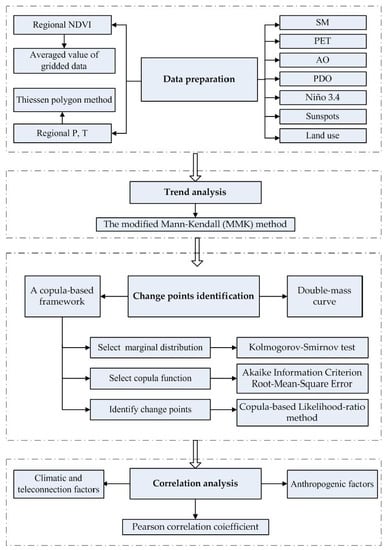
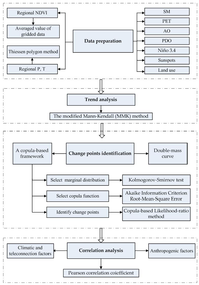
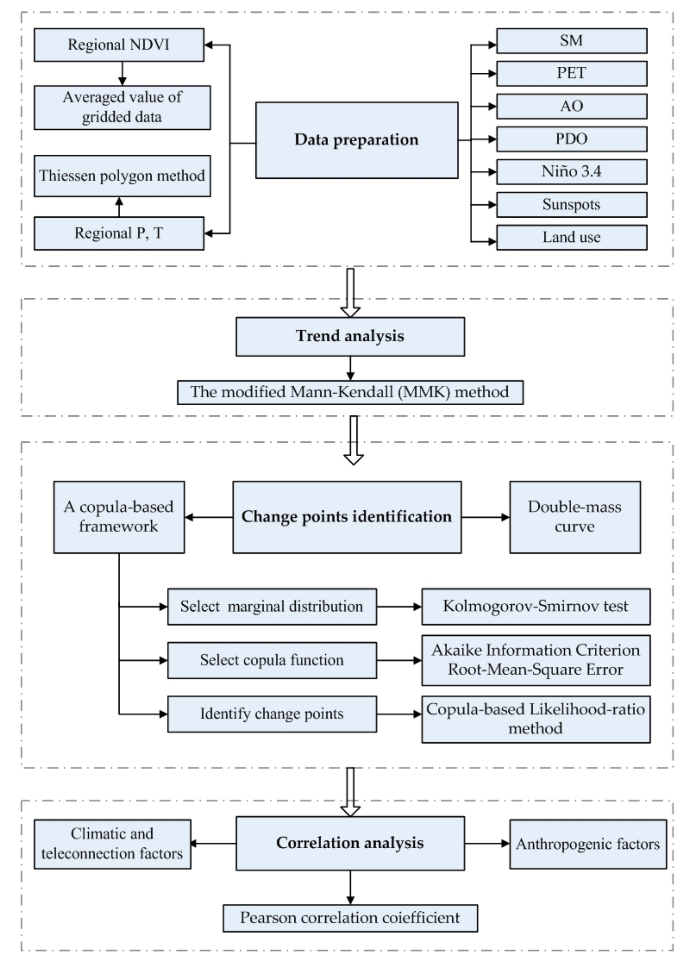
2. Materials and Methods
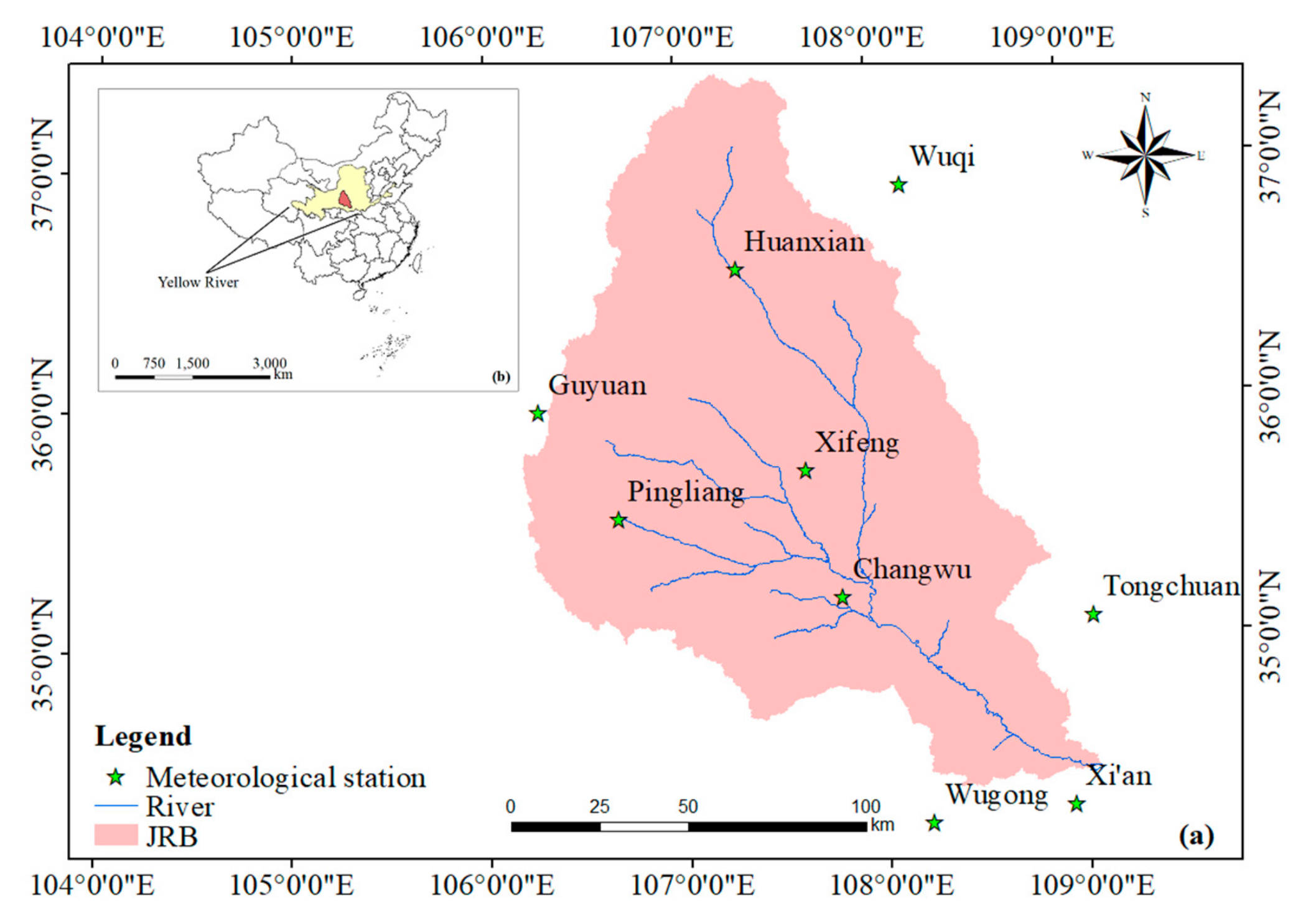
2.1. Study Area
2.2. Datasets
2.3. Trend Analysis
2.4. A Copula-Based Framework for Identifying the Change Points of the Relationship between NDVI and P/T
2.4.1. Marginal Distribution
2.4.2. Joint Distribution
2.4.3. Identify Change Points
2.5. Correlation Analysis
3. Results
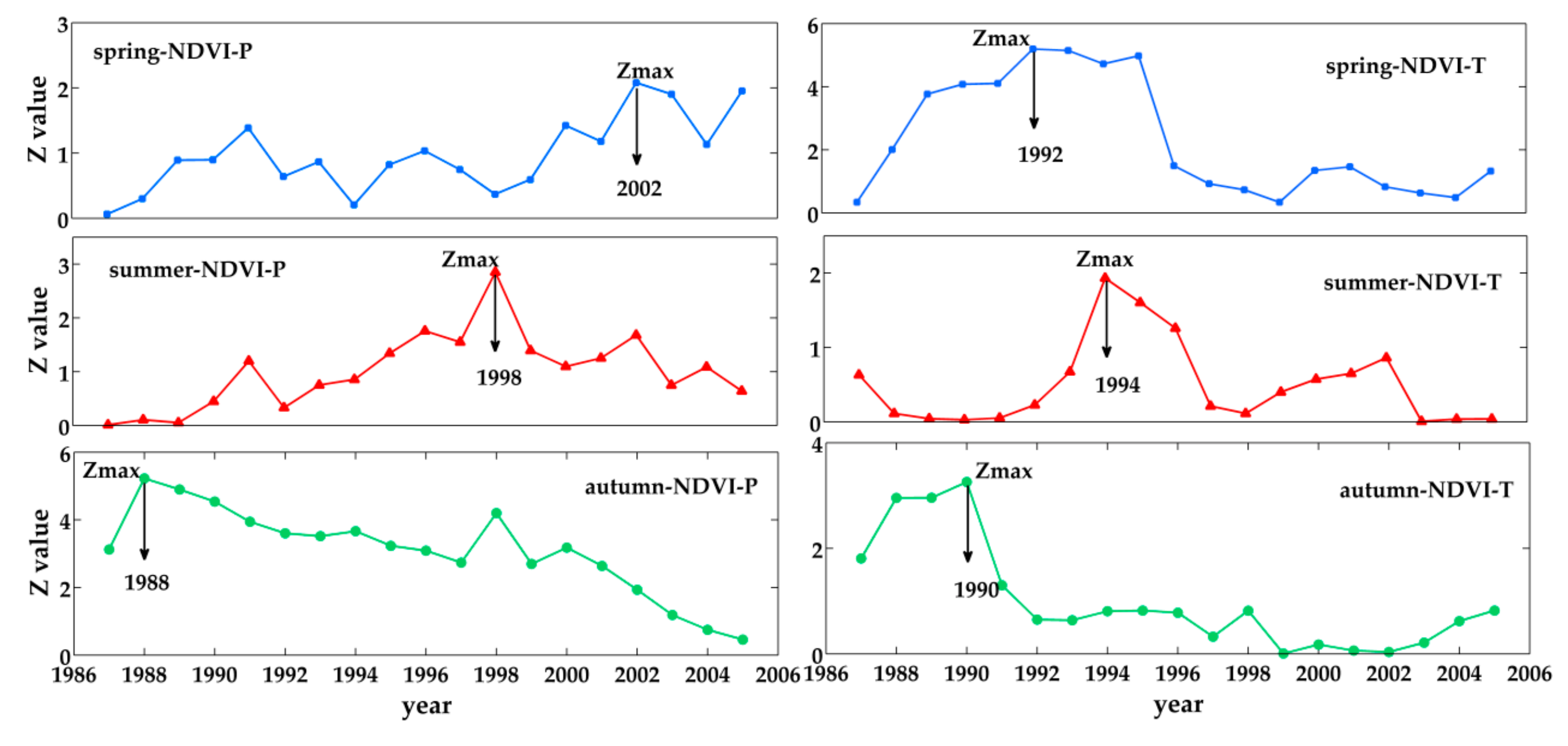
3.1. Temporal Change of Seasonal NDVI, Precipitation, and Temperature
3.2. The Selection of the Appropriate Marginal Distribution
3.3. The Selection of the Appropriate Copula Function
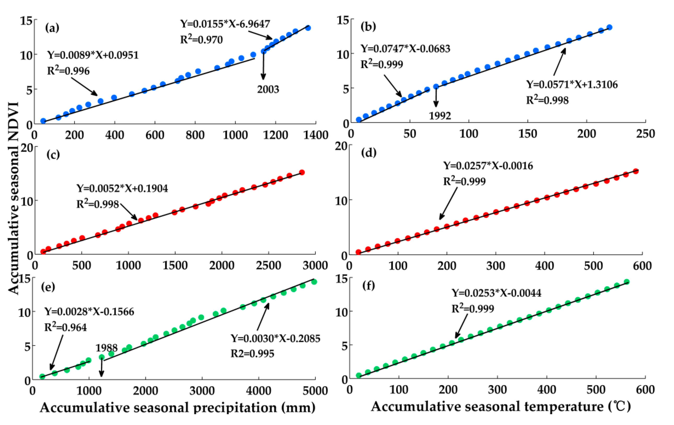
3.4. The Identification of Change Points in the Relationship between NDVI and P/T
4. Discussion
4.1. Methodology
4.2. The Climatic Drivers for the Variations of the Relationship between NDVI and P/T
4.3. The Anthropogenic Drivers for the Variations of the Relationship between NDVI and P/T
5. Conclusions
Author Contributions
Funding
Acknowledgments
Conflicts of Interest
References
- Peng, S.-S.; Piao, S.; Zeng, Z.; Ciais, P.; Zhou, L.; Li, L.Z.X.; Myneni, R.B.; Yin, Y.; Zeng, H. Afforestation in China cools local land surface temperature. Proc. Natl. Acad. Sci. USA 2014, 111, 2915–2919. [Google Scholar] [CrossRef] [PubMed] [Green Version]
- Piao, S.; Nan, H.; Huntingford, C.; Ciais, P.; Friedlingstein, P.; Sitch, S.; Peng, S.; Ahlström, A.; Canadell, J.G.; Cong, N.; et al. Evidence for a weakening relationship between interannual temperature variability and northern vegetation activity. Nat. Commun. 2014, 5, 1–7. [Google Scholar] [CrossRef] [PubMed]
- Pielke, R.A. Land use and climate change. Science 2005, 310, 1625–1626. [Google Scholar] [CrossRef] [PubMed]
- Sterling, S.M.; Ducharne, A.; Polcher, J. The impact of global land-cover change on the terrestrial water cycle. Nat. Clim. Change 2013, 3, 385–390. [Google Scholar] [CrossRef]
- Udelhoven, T.; Stellmes, M.; Barrio, G.; Hill, J. Assessment of rainfall and NDVI anomalies in Spain (1989–1999) using distributed lag models. Int. J. Remote Sens. 2009, 30, 1961–1976. [Google Scholar] [CrossRef]
- Huber, S.; Fensholt, R.; Rasmussen, K. Water availability as the driver of vegetation dynamics in the African Sahel from 1982 to 2007. Glob. Planet Change 2011, 76, 186–195. [Google Scholar] [CrossRef]
- Zhao, J.; Huang, S.; Huang, Q.; Wang, H.; Leng, G. Detecting the dominant cause of streamflow decline in the Loess Plateau of china based onthe latest budyko equation. Water 2018, 10, 1277. [Google Scholar] [CrossRef]
- Liu, L.; Huang, G.; Baetz, B.; Zhang, K. Environmentally-extended input-output simulation for analyzing production-based and consumption-based industrial greenhouse gas mitigation policies. Appl. Energy 2018, 232, 69–78. [Google Scholar] [CrossRef]
- Ciais, P.; Reichstein, M.; Viovy, N.; Granier, A.; Ogѐe, J.; Allard, V.; Aubinet, M.; Buchmann, N.; Bernhofer, C.; Carrara, A.; et al. Europe-wide reduction in primary productivity caused by the heat and drought in 2003. Nature 2005, 437, 529–533. [Google Scholar] [CrossRef]
- De Keersmaecker, W.; Lhermitte, S.; Tits, L.; Honnay, O.; Somers, B.; Coppin, P. A model quantifying global vegetation resistance and resilience to short-term climate anomalies and their relationship with vegetation cover cover. Glob. Ecol. Biogeogr. 2015, 24, 539–548. [Google Scholar] [CrossRef]
- Yang, Y.; Piao, S. Variations in grassland vegetation cover in relation to climatic factors on the Tibetan Plateau. J. Plant Ecol. 2006, 30, 1–8. [Google Scholar] [CrossRef]
- Wang, X.; Xie, H.; Guan, H.; Zhou, X. Different responses of MODIS-derived NDVI to root-zone soil moisture in semi-arid and humid regions. J. Hydrol. 2007, 340, 12–24. [Google Scholar] [CrossRef]
- Yu, Z.; Carlson, T.N.; Barron, E.J.; Schwartz, F.W. On evaluating the spatial-temporal variation of soil moisture in the Susquehanna river basin. Water Resour. Res. 2001, 37, 1313–1326. [Google Scholar] [CrossRef]
- Jiménez-Muñoz, J.C.; Sobrino, J.A.; Gillespie, A.; Sabol, D.; Gustafson, W.T. Improved land surface emissivities over agricultural areas using ASTER NDVI. Remote Sens. Environ. 2006, 103, 474–487. [Google Scholar] [CrossRef]
- Boegh, E.; Soegaard, H. Remote sensing based estimation of evapotranspiration rates. Int. J. Remote Sens. 2004, 25, 2535–2551. [Google Scholar] [CrossRef]
- Jiang, L.; Islam, S. Estimation of surface evaporation map over southern Great Plains using remote sensing data. Water Resour. Res. 2001, 37, 329–340. [Google Scholar] [CrossRef]
- Zeng, B.; Yang, T.B. Natural vegetation responses to warming climates in Qaidam Basin 1982–2003. Int. J. Remote Sens. 2009, 30, 5685–5701. [Google Scholar] [CrossRef]
- Yan, D.; Xu, T.; Girma, A.; Yuan, Z.; Weng, B.; Qin, T.; Do, P.; Yuan, Y. Regional correlation between precipitation and vegetation in the Huang-Huai-Hai river basin, China. Water 2017, 9, 557. [Google Scholar] [CrossRef]
- Shen, B.; Fang, S.; Li, G. Vegetation coverage changes and their response to meteorological variables from 2000 to 2009 in Naqu, Tibet, China. Can. J. Remote Sens. 2014, 40, 67–74. [Google Scholar] [CrossRef]
- Wen, Y.; Liu, X.; Pei, F.; Li, X.; Du, G. Non-uniform time-lag effects of terrestrial vegetation responses to asymmetric warming. Agric. For. Meteorol. 2018, 252, 130–143. [Google Scholar] [CrossRef]
- Ji, L.; Peters, A.J. Assessing vegetation response to drought in the northern Great Plains using vegetation and drought indices. Remote Sens. Environ. 2003, 87, 85–98. [Google Scholar] [CrossRef]
- Favretto, N.; Stringer, L.C.; Dougill, A.J.; Dallimer, M.; Perkins, J.S.; Reed, M.S.; Atlhopheng, J.R.; Mulale, K. Multi-criteria decision analysis to identify dryland ecosystem service trade-offs under different rangeland land uses. Ecosyst. Serv. 2016, 17, 142–151. [Google Scholar] [CrossRef]
- Jopke, C.; Kreyling, J.; Maes, J.; Koellner, T. Interactions among ecosystem services across Europe: Bagplots and cumulative correlation coefficients reveal synergies, trade-offs, and regional patterns. Ecol. Indic. 2015, 49, 46–52. [Google Scholar] [CrossRef]
- Jin, X.; Hao, Z.; Zhang, J. Study on the relation of frequency between flood and sediment in the middle Yellow River. J. Sediment Res. 2006, 3, 41–43. [Google Scholar] [CrossRef]
- Hao, R.; Yu, D.; Wu, J. Relationship between paired ecosystem services in the grassland and agro-pastoral transitional zone of China using the constraint line method. Agric. Ecosyst. Environ. 2017, 240, 171–181. [Google Scholar] [CrossRef]
- Lee, H.; McIntyre, N.; Wheater, H.; Young, A. Selection of conceptual models for regionalisation of the rainfall-runoff relationship. J. Hydrol. 2005, 312, 125–147. [Google Scholar] [CrossRef]
- Birkinshaw, S.J.; Bathurst, J.C. Model study of the relationship between sediment yield and river basin area. Earth Surf. Process. Landf. 2006, 31, 750–761. [Google Scholar] [CrossRef]
- Gu, D.; Ye, W.; Miao, B. Analysis of regional financial contagion based on vine copula method. J. Univ. Sci. Technol. Chin. 2013, 43, 737–744. [Google Scholar] [CrossRef]
- Huang, S.; Huang, Q.; Zhang, H.; Chen, Y.; Leng, G. Spatio-temporal changes in precipitation, temperature and their possibly changing relationship: A case study in the Wei River Basin, China. Int. J. Climatol. 2016, 36, 1160–1169. [Google Scholar] [CrossRef]
- Ye, W.; Miao, B.; Ma, Y. Analysis of sub-prime loan crisis contagion based on change point testing method of hazard function. Syst. Eng. Theory Pract. 2010, 30, 431–436. [Google Scholar] [CrossRef]
- Huang, S.; Huang, Q.; Chang, J.; Leng, G. Linkages between hydrological drought, climate indices and human activities: a case study in the Columbia River basin. Int. J. Climatol. 2016, 36, 280–290. [Google Scholar] [CrossRef]
- Han, Z.; Huang, S.; Huang, Q.; Leng, G.; Wang, H.; He, L.; Fang, W.; Li, P. Assessing GRACE-based terrestrial water storage anomalies dynamics at multi-timescales and their correlations with teleconnection factors in Yunnan Province, China. J. Hydrol. 2019. [Google Scholar] [CrossRef]
- Huang, S.; Li, P.; Huang, Q.; Leng, G.; Hou, B.; Ma, L. The propagation from meteorological to hydrological drought and its potential influence factors. J. Hydrol. 2017, 547, 184–195. [Google Scholar] [CrossRef]
- Li, J.; Fan, K.; Zhou, L. Satellite observations of El Niño impacts on eurasian spring vegetation greenness during the period 1982–2015. Remote Sens. 2017, 9, 628. [Google Scholar] [CrossRef]
- Cavazos, T. Using self-organizing maps to investigate extreme climate events: An application to wintertime precipitation in the Balkans. J. Clim. 2000, 13, 1718–1732. [Google Scholar] [CrossRef]
- Wu, B.; Wang, J. Possible impact of winter Arctic Oscillation on Siberian High, the East Asian winter monsoon and sea-ice extent. Adv. Atmos. Sci. 2002, 19, 297–320. [Google Scholar] [CrossRef]
- Zhao, J.; Huang, Q.; Chang, J.; Liu, D.; Huang, S.; Shi, X. Analysis of temporal and spatial trends of hydro-climatic variables in the Wei river basin. Environ. Res. 2015, 139, 55–64. [Google Scholar] [CrossRef] [PubMed]
- Liu, S.; Huang, S.; Xie, Y.; Wang, H.; Huang, Q.; Leng, G.; Li, P.; Wang, L. Spatial-temporal changes in vegetation coverage in a typical semi-humid and semi-arid region in China: Changing patterns, causes and implications. Ecol. Indic. 2019, 98, 462–475. [Google Scholar] [CrossRef]
- Li, X.; Wei, X.; Wei, N. Correlating check dam sedimentation and rainstorm characteristics on the Loess Plateau, China. Geomorphology 2016, 265, 84–97. [Google Scholar] [CrossRef]
- Xin, Z.; Yu, X.; Li, Q.; Lu, X.X. Spatiotemporal variation in rainfall erosivity on the Chinese Loess Plateau during the period 1956–2008. Reg. Environ. Change 2011, 11, 149–159. [Google Scholar] [CrossRef]
- Caocao, C.; Gaodi, X.; Lin, Z.; Yunfa, L. Analysis on Jinghe watershed vegetation dynamics and evaluation on its relation with precipitation. Acta Ecol. Sinica 2008, 28, 925–938. [Google Scholar] [CrossRef]
- Faisal, N.; Gaffar, A. Development of pakistan’s new area weighted rainfall using thiessen polygon method. Pak. J. Meteorol. 2012, 9, 107–116. [Google Scholar]
- Mitchell, J.M.; Dzerdzeevskii, B.; Flohn, H.; Hofmeyr, W.L.; Lamd, H.H.; Rao, K.N.; Wallen, C.C. Climate Change; Technical Note No. 79; World Meteorological Organization: Geneva, Switzerland, 1966; p. 79. [Google Scholar]
- Hamed, K.H.; Ramachandra Rao, A. A modified Mann-Kendall trend test for autocorrelated data. J. Hydrol. 1998, 204, 182–196. [Google Scholar] [CrossRef]
- Guo, Y.; Huang, S.; Huang, Q.; Wang, H.; Fang, W.; Yang, Y.; Wang, L. Assessing socioeconomic drought based on an improved Multivariate Standardized Reliability and Resilience Index. J. Hydrol. 2019, 568, 904–918. [Google Scholar] [CrossRef]
- Huang, S.; Chang, J.; Huang, Q.; Chen, Y. Spatio-temporal changes and frequency analysis of drought in the Wei river basin, china. Water Resour. Manag. 2014, 28, 3095–3110. [Google Scholar] [CrossRef]
- Mathier, L.; Perreault, L.; Bobee, B. The use of geometric and gamma-related distributions for frequency analysis of water deficit. Stoch. Hydrol. Hydraul. 1992, 6, 239–254. [Google Scholar] [CrossRef]
- Fang, W.; Huang, S.; Huang, G.; Huang, Q.; Wang, H.; Wang, L.; Zhang, Y.; Li, P.; Ma, L. Copulas-based risk analysis for inter-seasonal combinations of wet and dry conditions under a changing climate. Int. J. Climatol. 2018, 39, 2005–2021. [Google Scholar] [CrossRef]
- Wilks, D.S. Interannual variability and extreme-value characteristics of several stochastic daily precipitation models. Agric. For. Meteorol. 1999, 93, 153–169. [Google Scholar] [CrossRef]
- Ravens, B. An introduction to copulas. Technometrics 2000, 42, 317. [Google Scholar] [CrossRef]
- Genest, C.; Rivest, L.P. Statistical inference procedures for bivariate Archimedean copulas. J. Am. Stat. Assoc. 1993, 88, 1034–1043. [Google Scholar] [CrossRef]
- Akaike, H. A new look at the statistical model identification. IEEE Trans. Autom. Control 1974, 19, 716–723. [Google Scholar] [CrossRef]
- Costa Dias, A.D. Copula Inference for Finance and Insurance. Ph.D. Thesis, SWISS FEDERAL INSTITUTE OF TECHNOLOGY ZURICH, Zurich, Switzerland, 2004. [Google Scholar] [CrossRef]
- Gu, Z.; Duan, X.; Shi, Y.; Li, Y.; Pan, X. Spatiotemporal variation in vegetation coverage and its response to climatic factors in the Red river basin, China. Ecol. Indic. 2018, 93, 54–64. [Google Scholar] [CrossRef]
- Ning, T.; Liu, W.; Lin, W.; Song, X. NDVI variation and its responses to climate change on the Northern Loess Plateau of China from 1998 to 2012. Adv. Meteorol. 2015, 2015, 1–10. [Google Scholar] [CrossRef]
- Guo, A.; Chang, J.; Wang, Y.; Li, Y. Variation characteristics of rainfall-runoff relationship and driving factors analysis in Jinghe river basin in nearly 50 years. Trans. Chin. Soc. Agric. Eng. 2015, 31, 165–171. [Google Scholar] [CrossRef]
- Li, J.; Fan, K.; Xu, Z. Links between the late wintertime North Atlantic Oscillation and springtime vegetation growth over Eurasia. Clim. Dyn. 2016, 46, 987–1000. [Google Scholar] [CrossRef]
- Cho, M.H.; Lim, G.H.; Song, H.J. The effect of the wintertime Arctic Oscillation on springtime vegetation over the northern high latitude region. Asia Pac. J. Atmos. Sci. 2014, 50, 567–573. [Google Scholar] [CrossRef]
- Joiner, J.; Yoshida, Y.; Anderson, M.; Holmes, T.; Hain, C.; Reichle, R.; Koster, R.; Middleton, E.; Zeng, F. Global relationships among traditional reflectance vegetation indices (NDVI and NDII), evapotranspiration (ET), and soil moisture variability on weekly timescales. Remote Sens. Environ. 2018, 219, 339–352. [Google Scholar] [CrossRef] [Green Version]
- Kumar, T.V.L.; Rao, K.K.; Barbosa, H. Studies on spatial pattern of NDVI over India and its relationship with rainfall, air temperature, soil moisture adequacy and ENSO. Geofizika 2013, 30, 1–18. [Google Scholar] [CrossRef]
- Özger, M.; Mishra, A.K.; Singh, V.P. Scaling characteristics of precipitation data in conjunction with wavelet analysis. J. Hydrol. 2010, 395, 279–288. [Google Scholar] [CrossRef]
- Anyamba, A.; Eastman, J.R. Interannual variability of ndvi over africa and its relation to el niño/southern oscillation. Int. J. Remote Sens. 1996, 17, 2533–2548. [Google Scholar] [CrossRef]
- Gong, D.; Shi, P. Northern hemispheric NDVI variations associated with large-scale climate indices in spring. Int. J. Remote Sens. 2003, 24, 2559–2566. [Google Scholar] [CrossRef]
- Suzuki, R.; Tanaka, S.; Yasunari, T. Relationships between meridional profiles of satellite-derived vegetation index (ndvi) and climate over siberia. Int. J. Climatol. 2000, 20, 955–967. [Google Scholar] [CrossRef]
- Zhou, L.; Tucker, C.J.; Kaufmann, R.K.; Slayback, D.; Shabanov, N.V.; Myneni, R.B. Variations in northern vegetation activity inferred from satellite data of vegetation index during 1981–1999. J. Geophys. Res. 2001, 106, 20069–20083. [Google Scholar] [CrossRef]
- Wang, X.; Zhao, X.L.; Zhang, Z.X.; Yi, L.; Zuo, L.J.; Wen, Q.K.; Liu, F.; Xu, J.Y.; Hu, S.G.; Liu, B. Assessment of soil erosion change and its relationships with land use/cover change in China from the end of the 1980s to 2010. Catena 2016, 137, 256–268. [Google Scholar] [CrossRef]
- Yang, L.; Xie, G.; Zhen, L.; Guo, G.; Leng, Y.; Ge, Y. Spatial-temporal changes of land use in Jinghe watershed. Resour. Sci. 2005, 27, 26–32. [Google Scholar] [CrossRef]
- Pimentel, D.; Pimentel, M. Global environmental resources versus world population growth. Ecol. Econ. 2006, 59, 195–198. [Google Scholar] [CrossRef]
- Wang, S.; Fu, B.; Piao, S.; Lü, Y.; Ciais, P.; Feng, X.; Wang, Y. Reduced sediment transport in the yellow river due to anthropogenic changes. Nat. Geosci. 2015, 9, 38–41. [Google Scholar] [CrossRef]
- Li, Z.; Liu, W.Z.; Zhang, X.; Zheng, F. Impacts of land use change and climate variability on hydrology in an agricultural catchment on the Loess plateau of China. J. Hydrol. 2009, 377, 35–42. [Google Scholar] [CrossRef]
- Xiao, J.F. Satellite evidence for significant biophysical consequences of the ‘Grain for Green’ Program on the Loess Plateau in China. J. Geophys. Res. Biogeosci. 2014, 119, 2261–2275. [Google Scholar] [CrossRef]
- Tang, Q.; Xu, Y.; Liu, Y. Spatial difference of land use change in Loess plateau region. J. Arid Land Resour. Environ. 2010, 24, 15–21. [Google Scholar] [CrossRef]


| Season | NDVI | P | T |
|---|---|---|---|
| Spring | 0.8 | −1.0 | 2.6 ** |
| Summer | 1.4 | 0.3 | 3.6 ** |
| Autumn | 4.1 ** | 0.8 | 2.2 * |
| Seasons | Series | Gamma Distribution | GEV Distribution | Lognormal Distribution | |||
|---|---|---|---|---|---|---|---|
| H | P | H | P | H | P | ||
| Spring | NDVI | 0 | 0.56 | 0 | 0.84 | 0 | 0.58 |
| P | 0 | 0.92 | 0 | 0.96 | 0 | 0.70 | |
| T | 0 | 0.92 | 0 | 0.79 | 0 | 0.93 | |
| Summer | NDVI | 0 | 0.97 | 0 | 0.99 | 0 | 0.98 |
| P | 0 | 0.50 | 0 | 0.68 | 0 | 0.66 | |
| T | 0 | 0.79 | 0 | 0.95 | 0 | 0.81 | |
| Autumn | NDVI | 0 | 0.82 | 0 | 0.52 | 0 | 0.83 |
| P | 0 | 0.93 | 0 | 0.98 | 0 | 0.75 | |
| T | 0 | 0.62 | 0 | 0.94 | 0 | 0.64 | |
| Seasons | Series | Clayton | Frank | Gumbel | |||
|---|---|---|---|---|---|---|---|
| RMSE | AIC | RMSE | AIC | RMSE | AIC | ||
| Spring | NDVI-P | 0.029 | −203.27 | 0.024 | −215.21 | 0.032 | −198.52 |
| NDVI-T | 0.021 | −220.40 | 0.022 | −219.07 | 0.025 | −212.54 | |
| Summer | NDVI-P | 0.030 | −202.32 | 0.021 | −222.29 | 0.023 | −217.82 |
| NDVI-T | 0.032 | −197.77 | 0.024 | −214.24 | 0.032 | −197.77 | |
| Autumn | NDVI-P | 0.017 | −233.95 | 0.022 | −218.85 | 0.032 | −197.71 |
| NDVI-T | 0.033 | −196.74 | 0.030 | −201.06 | 0.040 | −185.00 | |
| Climatic and Teleconnection Factors | Spring | Summer | Autumn | |||
|---|---|---|---|---|---|---|
| ZNDVI-P | ZNDVI-T | ZNDVI-P | ZNDVI-T | ZNDVI-P | ZNDVI-T | |
| SM | −0.28 | −0.14 | −0.32 | 0.31 | −0.22 | 0.17 |
| PET | 0.20 | −0.24 | 0.46 * | 0.24 | −0.09 | −0.10 |
| AO | −0.65 ** | 0.72 ** | −0.43 | 0.38 | 0.71 ** | 0.58 ** |
| PDO | 0.61 ** | −0.71 ** | 0.51 * | −0.14 | −0.78 ** | −0.65 ** |
| Niño3.4 | −0.71 ** | 0.15 | 0.04 | 0.19 | 0.78 ** | 0.48 * |
| Sunspots | −0.72 ** | 0.41 | −0.31 | 0.39 | 0.74 ** | 0.43 |
| EIA | 0.26 | 0.09 | 0.61 ** | 0.39 | 0.41 | 0.84 ** |
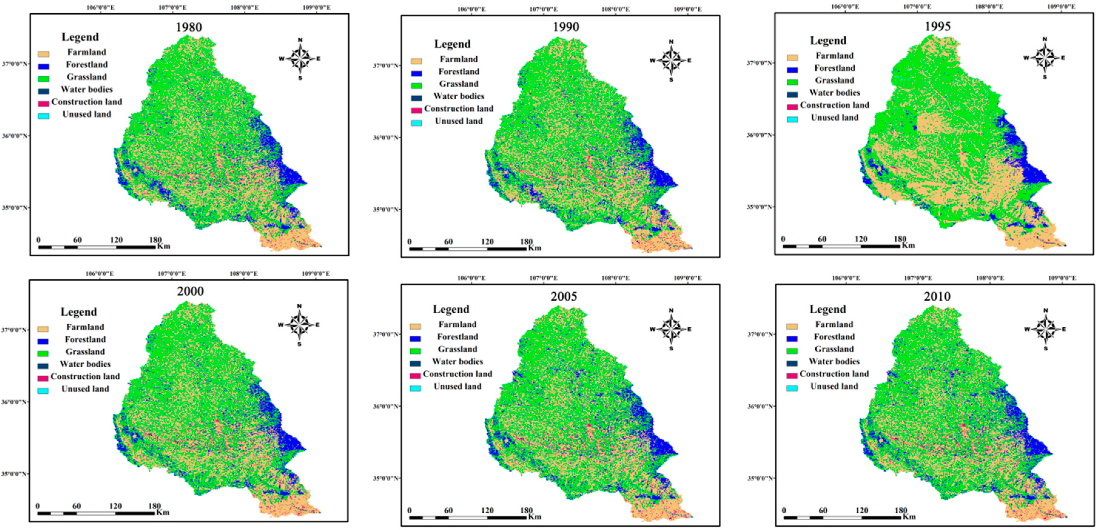
| Year | Farmland | Forestland | Grassland | Water Bodies | Construction Land | Unused Land | ||||||
|---|---|---|---|---|---|---|---|---|---|---|---|---|
| Area km2 | Ratio % | Area km2 | Ratio % | Area km2 | Ratio % | Area km2 | Ratio % | Area km2 | Ratio % | Area km2 | Ratio % | |
| 1980 | 19,901 | 44.41 | 4179 | 9.33 | 19,829 | 44.25 | 215 | 0.48 | 690 | 1.54 | 1 | 0 |
| 1990 | 19,960 | 44.54 | 4239 | 9.46 | 19,738 | 44.04 | 205 | 0.46 | 670 | 1.49 | 3 | 0.01 |
| 1995 | 20,172 | 45.01 | 4023 | 8.98 | 19,645 | 43.84 | 192 | 0.43 | 721 | 1.61 | 62 | 0.14 |
| 2000 | 19,865 | 44.33 | 4026 | 8.98 | 19,946 | 44.51 | 213 | 0.47 | 765 | 1.71 | 0 | 0 |
| 2005 | 19,499 | 43.51 | 4439 | 9.9 | 19,815 | 44.22 | 212 | 0.47 | 847 | 1.89 | 3 | 0.01 |
| 2010 | 19,426 | 43.35 | 4470 | 9.97 | 19,847 | 44.29 | 209 | 0.47 | 860 | 1.92 | 3 | 0.01 |
© 2019 by the authors. Licensee MDPI, Basel, Switzerland. This article is an open access article distributed under the terms and conditions of the Creative Commons Attribution (CC BY) license (http://creativecommons.org/licenses/by/4.0/).
Share and Cite
Zhao, J.; Huang, S.; Huang, Q.; Wang, H.; Leng, G.; Peng, J.; Dong, H. Copula-Based Abrupt Variations Detection in the Relationship of Seasonal Vegetation-Climate in the Jing River Basin, China. Remote Sens. 2019, 11, 1628. https://doi.org/10.3390/rs11131628
Zhao J, Huang S, Huang Q, Wang H, Leng G, Peng J, Dong H. Copula-Based Abrupt Variations Detection in the Relationship of Seasonal Vegetation-Climate in the Jing River Basin, China. Remote Sensing. 2019; 11(13):1628. https://doi.org/10.3390/rs11131628
Chicago/Turabian StyleZhao, Jing, Shengzhi Huang, Qiang Huang, Hao Wang, Guoyong Leng, Jian Peng, and Haixia Dong. 2019. "Copula-Based Abrupt Variations Detection in the Relationship of Seasonal Vegetation-Climate in the Jing River Basin, China" Remote Sensing 11, no. 13: 1628. https://doi.org/10.3390/rs11131628