Article

Estimation of Land Surface Heat Fluxes Based on Landsat 7 ETM+ Data and Field Measurements over the Northern Tibetan Plateau

1
Laboratory for Atmospheric Observation and Climate Environment Research, School of Earth and Space Sciences, University of Science and Technology of China, Hefei 230026, China
2
CAS Center for Excellence in Comparative Planetology, Hefei 230026, China
3
Jiangsu Collaborative Innovation Center for Climate Change, Nanjing 210023, China
4
Key Laboratory of Tibetan Environment Changes and Land Surface Processes, Institute of Tibetan Plateau Research, Chinese Academy of Science, Beijing 100101, China
5
CAS Center for Excellence in Tibetan Plateau Earth Sciences, Beijing 100101, China
6
College of Earth and Planetary Sciences, University of Chinese Academy of Science, Beijing 100049, China
*
Author to whom correspondence should be addressed.
Remote Sens. 2019, 11(24), 2899; https://doi.org/10.3390/rs11242899
Submission received: 29 October 2019 / Revised: 23 November 2019 / Accepted: 4 December 2019 / Published: 5 December 2019
(This article belongs to the Special Issue Observations, Modeling, and Impacts of Climate Extremes)

Abstract

:
Land surface heat fluxes consist of the net radiation flux, soil heat flux, sensible heat flux, and latent heat flux. The estimation of these fluxes is essential to the study of energy transfer in land–atmosphere systems. In this paper, Landsat 7 ETM+ SLC-on data were applied to estimate the land surface heat fluxes on the northern Tibetan Plateau using the SEBS (surface energy balance system) model, in combination with the calculation of field measurements at CAMP/Tibet (Coordinated Enhanced Observing Period (CEOP) Asia–Australia Monsoon Project on the Tibetan Plateau) automatic weather stations based on the combinatory method (CM) for comparison. The root mean square errors between the satellite estimations and the CM calculations for the net radiation flux, soil heat flux, sensible heat flux, and latent heat flux were 49.2 W/m2, 46.3 W/m2, 68.2 W/m2, and 54.9 W/m2, respectively. The results reveal that land surface heat fluxes all present significant seasonal variability. Apart from the sensible heat flux, the satellite-estimated net radiation flux, soil heat flux, and latent heat flux exhibited a trend of summer > spring > autumn > winter. In summer, spring, autumn, and winter, respectively, the median values of the net radiation flux (631.8 W/m2, 583.0 W/m2, 404.4 W/m2, 314.3 W/m2), soil heat flux (40.9 W/m2, 37.9 W/m2, 26.1 W/m2, 20.5 W/m2), sensible heat flux (252.7 W/m2, 219.5 W/m2, 221.4 W/m2, 204.8 W/m2), and latent heat flux (320.1 W/m2, 298.3 W/m2, 142.3 W/m2, 75.5 W/m2) exhibited distinct seasonal diversity. From November to April, the in situ sensible heat flux is higher than the latent heat flux; the opposite is true between June and September, leaving May and October as transitional months. For water bodies, alpine meadows and other main underlying surface types, sensible and latent heat flux generally present contrasting and complementary spatial distributions. Due to the 15–60 m resolution of the Landsat 7 ETM+ data, the distribution of land surface heat fluxes can be used as an indicator of complex underlying surface types over the northern Tibetan Plateau.

Graphical Abstract

1. Introduction

Land surface heat fluxes include net radiation flux, soil heat flux, sensible heat flux, and latent heat flux, which are components of land surface energy balance [1]. Net radiation flux reflects the total energy budget over the land surface, and soil heat flux depicts the heat absorption beneath the ground. Sensible heat flux and latent heat flux represent the heat transfer between the land surface and the atmosphere due to temperature differences and water vapor phase transitions, respectively. Land surface heat fluxes are essential to land–atmosphere interactions in the atmospheric boundary layer. The variability of land surface heat fluxes may originate from land use land cover changes and natural variations, which could serve as an indicator of land cover change over both the artificial and natural underlying surface [2]. Land surface heat fluxes can directly influence the land surface temperature, which is an important driver of local warming [3,4]. Furthermore, variations in land surface heat fluxes will also have an impact on the atmospheric circulation and climate change, which are of great significance to the study of energy exchange in land–atmosphere interactions [5,6,7,8,9].
The Tibetan Plateau, which is located in the southwest of China and covers an area of approximately 2.6 million square kilometers with an average elevation over 4000 m above mean sea level, is also called the ‘Roof of the World’ and ‘The Third Pole’. The land surface processes over the Tibetan Plateau play an important role in the Asian–Australian monsoon circulation and the global climate change. Due to its unique location and harsh environment, the land surface heat fluxes over the Tibetan Plateau have distinct characteristics.
Pioneering works have been done by some researchers on the observation and estimation of land surface heat fluxes on the Tibetan Plateau by satellite remote sensing [10,11,12,13,14,15,16,17,18]. Ma et al. [10] used NOAA-14 AVHRR data and field measurements to derive the spatial distributions of land surface net radiation flux and soil heat flux in the GAME-Tibet (Global Energy and Water Cycle Experiment (GEWEX) Asian Monsoon Experiment on the Tibetan Plateau) region of the Tibetan Plateau. The estimation of land surface heat fluxes based on satellite data with 10–100 m spatial resolutions has already been tested on the Mt. Everest region. Chen et al. [15] estimated the land surface energy fluxes in the Mt. Everest region by using Landsat TM/ETM+ data. Han et al. [17] used ASTER (Advanced Spaceborne Thermal Emission and Reflection Radiometer) data to estimate the regional land surface heat fluxes in the Mt. Everest region.
In previous studies, the most commonly used satellite data for estimates of land surface heat fluxes over the Tibetan Plateau were images with spatial resolutions of 1–10 km [10,12,14,16,18]. Estimations of land surface heat fluxes based on satellite data with 10–100 m spatial resolutions have been applied to the Mt. Everest region [15,17], but have rarely involved the northern Tibetan Plateau [11,13]. The spatial resolutions of MODIS (Moderate Resolution Imaging Spectroradiometer) data and AVHRR (Advanced Very-High-Resolution Radiometer) data, for example, are only 250–1000 m and 1000–4000 m, respectively, making it difficult to accurately obtain the land surface characteristic parameters and the turbulent heat flux data for land–atmosphere energy exchange from the micro-scale to meso-scale. In comparison, Landsat 7 ETM+ data have a spatial resolution of 15–60 m (Table 4), which would be more suitable for remote sensing analysis over regions at 10–100 km scales. Additionally, corresponding to the satellite estimation results, the characteristics of in situ land surface heat fluxes, which can be derived from time series of multi-level ground-based observations, are rarely taken into consideration.
In this paper, Landsat 7 ETM+ SLC-on data, ITPCAS (Institute of Tibetan Plateau Research, Chinese Academy of Sciences) forcing data [19,20] and CAMP/Tibet (Coordinated Enhanced Observing Period (CEOP) Asia–Australia Monsoon Project on the Tibetan Plateau) [21] observation data were used. Based on ground-based observations, the combinatory method (CM) [22,23,24] was used to calculate and analyze the variations of in situ land surface heat fluxes at multiple temporal scales. By using satellite remote sensing data as inputs, the SEBS (surface energy balance system) model [25] was applied to estimate and analyze the seasonal variations and spatial distributions of land surface heat fluxes, and the results were compared with those of the ground-based calculations. The rest of this paper is organized as follows. Section 2 briefly introduces the study area and the datasets, and outlines the basic principles of the CM and the SEBS model. Section 3 presents the research results and analysis; Section 4 discusses the advantages and limitations; and Section 5 presents the main conclusions.

2. Materials and Methods

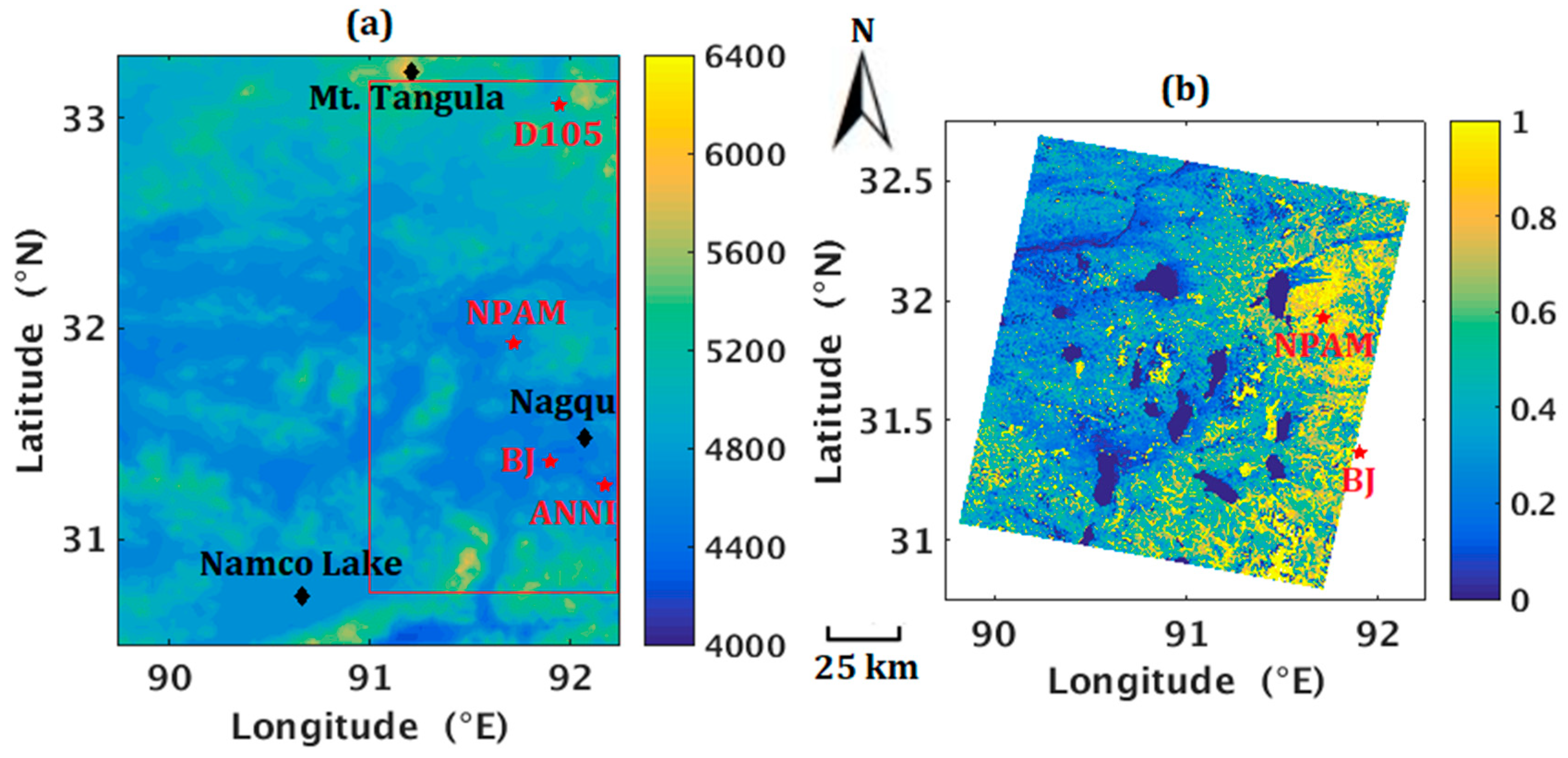
2.1. Study Area and Data

2.1.1. Study Area

The elevation variation of the study area and the fractional vegetation cover distribution of one scene (on June 13, 2001) in the Landsat 7 ETM+ data (Path 138/Row 038) are shown in Figure 1. The fractional vegetation cover (fvc) was estimated using the normalized squared NDVI (Normalized Difference Vegetation Index) relation from Equation (13). The study area is located in the northern Tibetan Plateau, and the location of the CAMP/Tibet area is inside the red rectangular border seen in Figure 1a. In the study area, the fractional vegetation cover was generally higher in the east and lower in the west, reaching 1 or 0 over the land surface of dense vegetation or water bodies, respectively. With the Nagqu region in the east, Mt. Tangula in the north, and Namco Lake in the south, the area contains a distribution of lakes, alpine and subalpine meadows, alpine and subalpine plains, and other complex underlying surface types over 4000 m.

2.1.2. Ground-Based Data

The in situ measurements used in this paper were from automatic weather stations (AWS) including ANNI, BJ, D105, and NPAM in CAMP/Tibet (Table 1). The time span of CAMP/Tibet ground-based data used in this paper was from 2001 to 2003, which is in accordance with the Landsat 7 ETM+ SLC-on satellite data used in this paper. The CAMP/Tibet data can be obtained from http://en.tpedatabase.cn/portal/MetaDataInfo.jsp?MetaDataId=217.
Due to the lack of in situ eddy correlation flux observation data from 2001 to 2003, the sensible heat flux and latent heat flux cannot be derived via the eddy correlation method, thus the combinatory method [22,23,24] was used as a substitute to calculate the surface heat fluxes. The combinatory method is the algorithm for calculating land surface soil heat flux, sensible heat flux, and latent heat flux based on ground-based multi-layer measurements. It was first proposed by Thom et al. [22], and then developed by Hu et al. [23]. This method combines the energy balance method and the aerodynamic method, so it was called the combinatory method (CM) [23]. In the CM, seven meteorological elements, wind speed, air temperature, air pressure, relative humidity, radiation balance components (downward shortwave radiation, upward shortwave radiation, downward longwave radiation, and upward longwave radiation), soil temperature, and soil heat flux (z depth, Table 2) at different observation levels are used as inputs to calculate the net radiation flux, soil heat flux, sensible heat flux, and latent heat flux at the ground surface. Information on these seven meteorological elements measured at automatic weather stations of CAMP/Tibet is shown in Table 2. Taking the measured data of the above meteorological elements as inputs, the in situ land surface net radiation flux, soil heat flux (at z = 0), sensible heat flux, and latent heat flux can be calculated by the CM.

2.1.3. Satellite Data

The time span of the Landsat 7 ETM+ SLC-on data used in this paper was from June 2001 to April 2003. As CAMP/Tibet started in 2001 and the Scan Line Corrector (SLC) onboard Landsat 7 suddenly broke on May 31, 2003, the satellite data before 2001 and those after May 31, 2003 (i.e., Landsat 7 ETM+ SLC-off data) were not used in this paper. For quality control of the satellite data, satellite images with mean cloudiness over 40% were excluded from this study. A total of 13 scenes of Landsat 7 ETM+ SLC-on data were used in this study (Table 3). The information of Landsat 7 ETM+ bands is listed in Table 4. The Landsat 7 ETM+ SLC-on data can be acquired from http://www.gscloud.cn/sources/list_dataset/242?cdataid=263&pdataid=10&datatype=L7slc-on#dlv=Wzg4LFswLDEwLDEsMF0sW1siZGF0YWRhdGUiLDBdXSxbXSw5OV0%3D. The Landsat 7 ETM+ SLC-on data can also be acquired from https://glovis.usgs.gov/.
In order to use the SEBS model to estimate land surface heat fluxes, the meteorological variables and land surface characteristic parameters in the study area should be obtained as model inputs. Among them, the meteorological variables of wind speed, air temperature, air pressure, and specific humidity for this study came from the ITPCAS forcing data. The ITPCAS forcing data, also called the China Meteorological Forcing Data, is a gridded reanalysis data product based on measurements of 740 operational stations of the China Meteorological Administration, TRMM (Tropical Rainfall Measuring Mission) satellite precipitation analysis data (3B42), GEWEX-SRB (Global Energy and Water Exchanges - Surface Radiation Budget) data, and GLDAS (Global Land Data Assimilation System) data. The ITPCAS forcing data have a temporal resolution of three hours and a spatial resolution of 0.1° × 0.1°, respectively. The ITPCAS forcing data can be accessed from http://en.tpedatabase.cn/portal/MetaDataInfo.jsp?MetaDataId=202. In order to integrate with the Landsat image, a temporal linear interpolation was executed to derive the variable values of ITPCAS forcing data at overpass times of the Landsat 7 scenes, then a spatial bilinear interpolation was implemented for the ITPCAS forcing data to convert the original grid point coordinates to the Landsat pixel. Subsequently, the Landsat 7 ETM+ SLC-on data and the converted ITPCAS forcing data were used as the inputs of the SEBS model for estimation of the land surface heat fluxes. The satellite images took 27 seconds to scan at approximately 04:15 UTC (12:15 Beijing Standard Time, BST). For validation of the satellite results, a temporal linear interpolation was also applied to the in situ results to obtain values for 12:15 BST.

2.2. Method and Model

2.2.1. The Combinatory Method (CM)

The main methods used to calculate land surface sensible heat flux and latent heat flux by using ground-based observation data include the eddy correlation method, the profile method, the aerodynamic method, the energy balance method (the Bowen ratio method), the H (sensible heat flux) deduction method, the CM, and the optical method. The CM was named for its characteristic combination of the aerodynamic method and the energy balance method [22,23]. Compared with the aerodynamic method, in addition to wind speed, air temperature, air pressure, and relative humidity, the simultaneous gradient observation data of soil temperature and soil heat flux (z depth) of the meteorological elements are also needed for the CM. The CM can calculate land surface sensible heat flux and latent heat flux without determination of the Monin–Obukhov universal function [26] in advance (Equations (2) and (3)); compared with the energy balance method, the CM applies the surface energy balance equation for stability correction of the calculated sensible heat flux and latent heat flux (Equations (6)–(8)) to obtain relatively precise calculation values.
The specific steps for calculating land surface sensible heat flux and latent heat flux by the CM are as follows.
First, the measured soil heat flux at z depth Gz and the gradient observational timeseries of the soil temperature were used to integrate layer by layer from a depth of z to the land surface to calculate the surface soil heat flux G0.
G 0 = G z + 0 z C s T t d z
where Cs is the volumetric heat capacity of soil [J·K−1·m−3], which can be seen as a constant in a 1–100 m scale region; and ∂T/∂t is the time change rate of soil temperature, which can be calculated according to the time series of soil temperature at each layer.
Second, the surface sensible heat flux H0 and the surface latent heat flux LE0 were calculated; these parameters require stability correction.
H 0 = ρ · c p · k 2 · Z A 2 · u z · θ z
L E 0 = ρ · L · k 2 · Z A 2 · u z · q z
where k is von Karman’s constant; ρ is the air density (derived from air pressure and air temperature); cp is specific heat capacity at constant pressure [J·K−1·kg−1]; L is the latent heat of water vaporization [J·K−1·kg−1]; ZA is the geometric mean of observation heights of two layers (Equation (4)); θ is the potential temperature; and q is the specific humidity (Equation (5)).
Z A = Z i · Z i + 1
q = 0.622 e p 0.378 e
Then, the stability influence function F was calculated, which served as the stability correction for H0 and LE0 for the derivation of land surface sensible heat flux H and latent heat flux LE (Equations (6)–(8)).
F = R n G 0 H 0 + L E 0
H = F · H 0
L E = F · L E 0

2.2.2. The SEBS (Surface Energy Balance System) Model

Based on the land surface energy balance equation and Monin–Obukhov similarity theory [26], the SEBS model [25] applies a parameterization scheme for the estimation of surface parameters and surface sensible heat flux and latent heat flux.
The specific steps for estimating land surface heat fluxes by the SEBS model are as follows.
The land surface energy balance equation is generally written as:
R n = G 0 + H + L E
The net radiation flux Rn is calculated from [27,28,29,30]:
R n = S W D S W U + L W D L W U
R n = ( 1 α ) S W D + L W D ε s · σ · T s 4
where α is surface albedo; εs is surface emissivity; and Ts is surface temperature.
The soil heat flux G0 can be estimated directly from the net radiation flux [31]:
G 0 = R n · [ f v c · r c + ( 1 f v c ) · r s ]
where rc and rs are the ratio of soil heat flux and net radiation flux in the canopy area and bare soil area, respectively; fvc is the fractional vegetation cover, which can be derived from NDVI; and NDVI is calculated from the reflectance of Band 3 and Band 4 of Landsat 7 (Equation (14)). It should be noted that for the water area, G0 is calculated as G 0 = 0.5 · R n [15,32].
f v c = ( N D V I N D V I m i n N D V I m a x N D V I m i n ) 2
N D V I = ρ 4 ρ 3 ρ 4 + ρ 3
To calculate the sensible heat flux H, three equations need to be solved simultaneously:
L = ρ · c p · θ v · u * 3 k · g · H
u * = k · u · [ l n ( z d 0 z 0 m ) Ψ m ( z d 0 L ) + Ψ m ( z 0 m L ) ] 1
H = k · u * · ρ · c p · ( θ 0 θ a ) · [ l n ( z d 0 z 0 h ) Ψ h ( z d 0 L ) + Ψ h ( z 0 h L ) ] 1
where L is the Obukhov length; cp is the specific heat capacity at constant pressure; θv is the virtual potential temperature; u* is the friction velocity; k is von Karman’s constant; z is the near-surface reference height; u is the horizontal wind speed at reference height; d0 is the zero plane displacement height; z0m is the roughness height for momentum transfer; z0h is the roughness height for heat transfer; θ0 is the surface potential temperature; θa is the air potential temperature at reference height; and Ψm and Ψh are stability correction functions for momentum flux and heat flux, respectively [33,34,35]. The mathematical expressions of Ψm and Ψh used in the SEBS model are written as follows:
Ψ m ( ζ ) = { 2 · ln ( 1 + X 2 ) + ln ( 1 + X 2 2 ) 2 · arctan ( X ) + π 2         ( ζ < 0 ) 5 · ζ         ( 0 ζ < 0.5 ) 0.5 ζ 2 4.25 ζ 7 · ln ( ζ ) 0.852         ( 0.5 ζ < 10 ) ln ( ζ ) 0.76 · ζ 12.093         ( ζ 10 )
Ψ h ( ζ ) = { 2 · ln ( 1 + X 2 2 )         ( ζ < 0 ) 5 · ζ         ( 0 ζ < 0.5 ) 0.5 ζ 2 4.25 ζ 7 · ln ( ζ ) 0.852         ( 0.5 ζ < 10 ) ln ( ζ ) 0.76 · ζ 12.093         ( ζ 10 )
X = ( 1 16 · ζ ) 0.25
There are three unknown variables, in the three equations above L, u*, and H (Equations (15)–(17)), which constitute a closed equation set. Due to the implicit functional relationship of these three unknown variables, the three equations are solved via iteration: First, assume ζ = 0 for the neutral stability condition. We can find that Ψm(ζ) = 0 and Ψh(ζ) = 0 according to Equations (18)–(20). Consequently, we obtain the initial guesses for u* and H (Equations (16) and (17)). Then, we can solve the initial L from u* and H (Equation (15)). Afterward, the next u* is solved from L (Equation (16)), and the next H is solved from L and u* (Equation (17)), and then the next L is solved from u* and H again. Through the iteration procedure above (approximately 10–100 iterations), the values of L, u*, and H will gradually approach their numerical solutions. After the sensible heat flux H is worked out, the latent heat flux LE can be derived by the wet-limit estimation [25].

3. Results

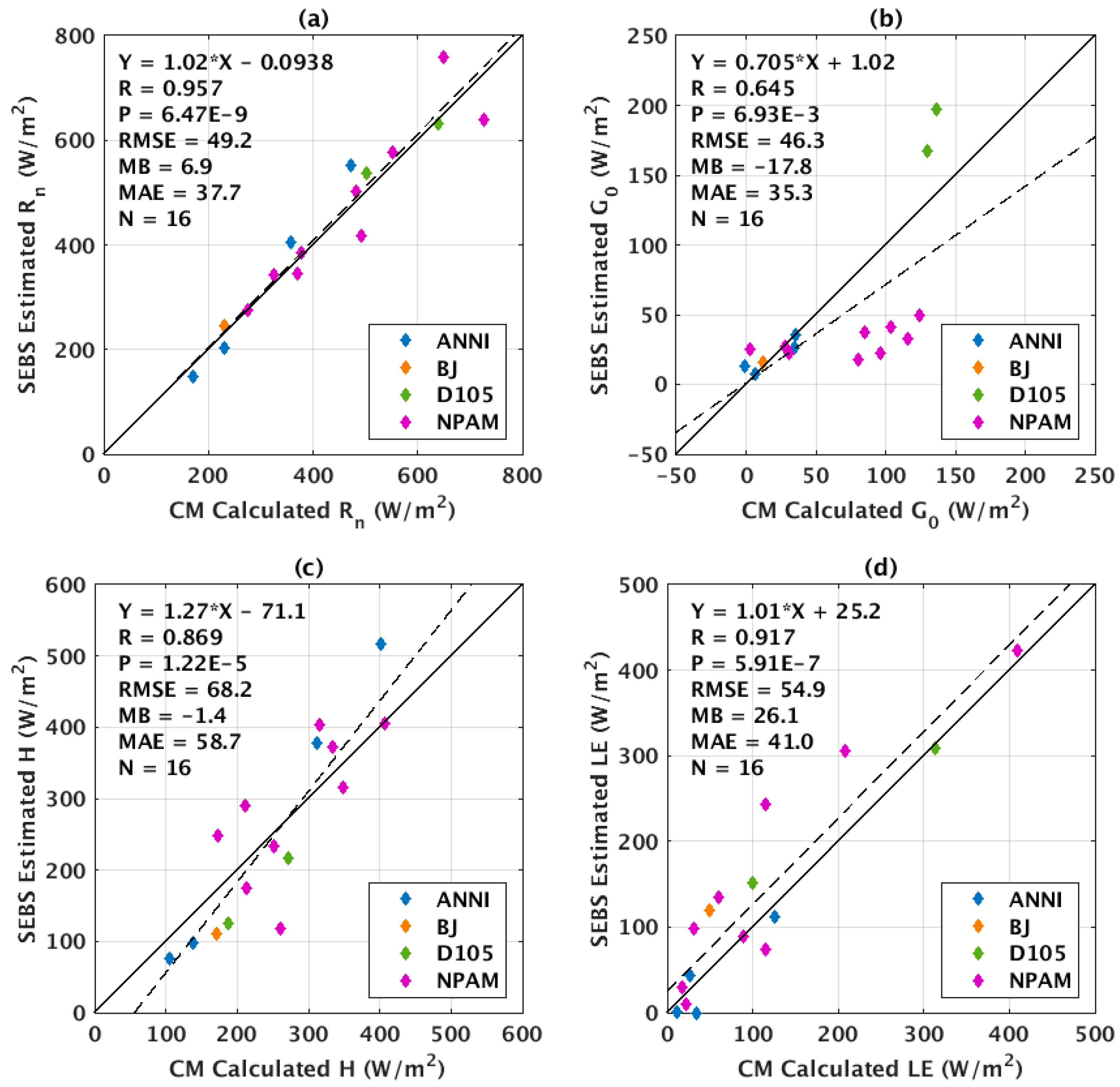
3.1. Comparison of SEBS and CM Results

The CAMP/Tibet data is point-based and the Landsat 7 ETM+ SLC-on data is pixel-based. The scale mismatch issue should be elaborated here. Actually, the underlying surface of each CAMP/Tibet AWS (ANNI, BJ, D105, NPAM) can be thought of as relatively homogeneous. Furthermore, Landsat ETM+ has a much higher spatial resolution, which varies from 15 m to 60 m. The scale mismatch during the validation process can be minimized. In the validation, two-dimensional coordinate (longitude, latitude) of each CAMP/Tibet AWS would fall inside the area of four Landsat pixels that are the nearest. In order to integrate the CAMP/Tibet field measurements and Landsat images, for each variable, we made an average of four pixels around each CAMP/Tibet AWS location as the satellite estimation value.
The scatterplots of energy balance components for SEBS estimation from satellite data and CM calculation from field measurements are shown in Figure 2. Four statistical indicators, RMSE (root mean square error), MB (mean bias), MAE (mean absolute error), and R (Pearson correlation coefficient) were calculated to measure the degree of closeness of ground-based and satellite results (Equations (21)–(24)). For net radiation flux and soil heat flux, RMSE = 49.2 W/m2 and 46.3 W/m2, MAE = 37.7 W/m2 and 35.3 W/m2, and MB = 6.9 W/m2 and −17.8 W/m2, respectively. For sensible heat flux, RMSE = 68.2 W/m2, MAE = 58.7 W/m2, and MB = −1.4 W/m2, indicating that the satellite estimation was lower than the in situ calculation. For latent heat flux, RMSE = 54.9 W/m2, MAE = 41.0 W/m2, and MB = 26.1 W/m2, indicated that the satellite estimation was higher than the in situ calculation. The Pearson correlation coefficients of satellite and in situ results for net radiation flux, soil heat flux, sensible heat flux, and latent heat flux were 0.957, 0.645, 0.869, and 0.917, respectively. The p-values for net radiation flux Rn, soil heat flux G0, sensible heat flux H, and latent heat flux LE were 6.47E-9, 6.93E-3, 1.22E-5, and 5.91E-7, respectively. Since these p-values were all less than 0.01, the Pearson correlation coefficients for Rn, G0, H, and LE were all of statistical significance. The differences in the calculation methods for sensible heat flux [23,25] and the input data from ground-based and satellite estimation may explain the RMSE, MB, and MAE of the energy balance components above. Additionally, due to the commonly negative correlation between sensible heat flux and latent heat flux, the underestimation of sensible heat flux may result in the overestimation of latent heat flux.
M B = 1 N · i = 1 N ( y i x i )
M A E = 1 N · i = 1 N | y i x i |
R M S E = 1 N · i = 1 N ( y i x i ) 2
R = i = 1 N ( ( x i x ¯ ) · ( y i y ¯ ) ) i = 1 N ( ( x i x ¯ ) 2 ) · i = 1 N ( ( y i y ¯ ) 2 )

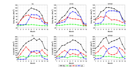
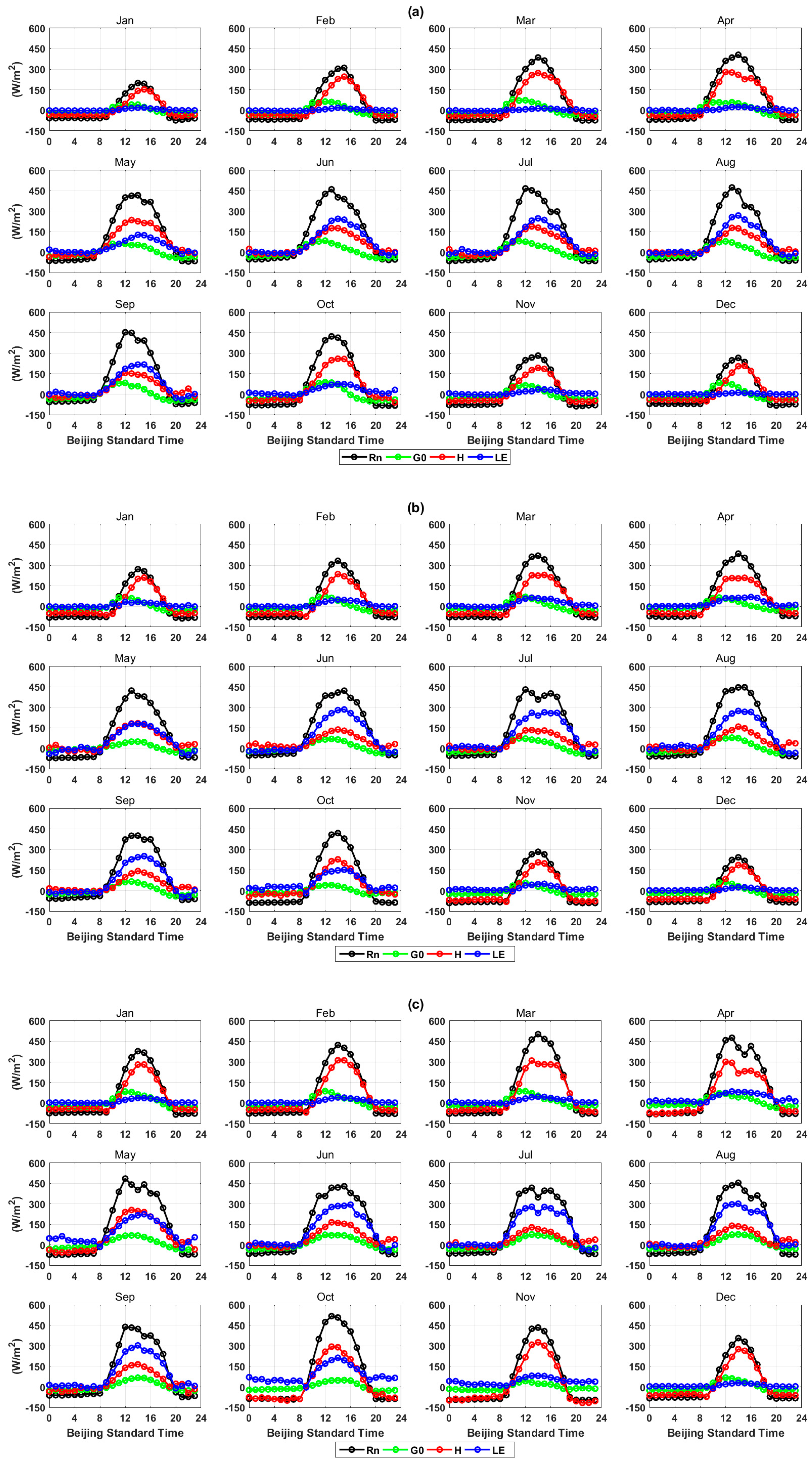
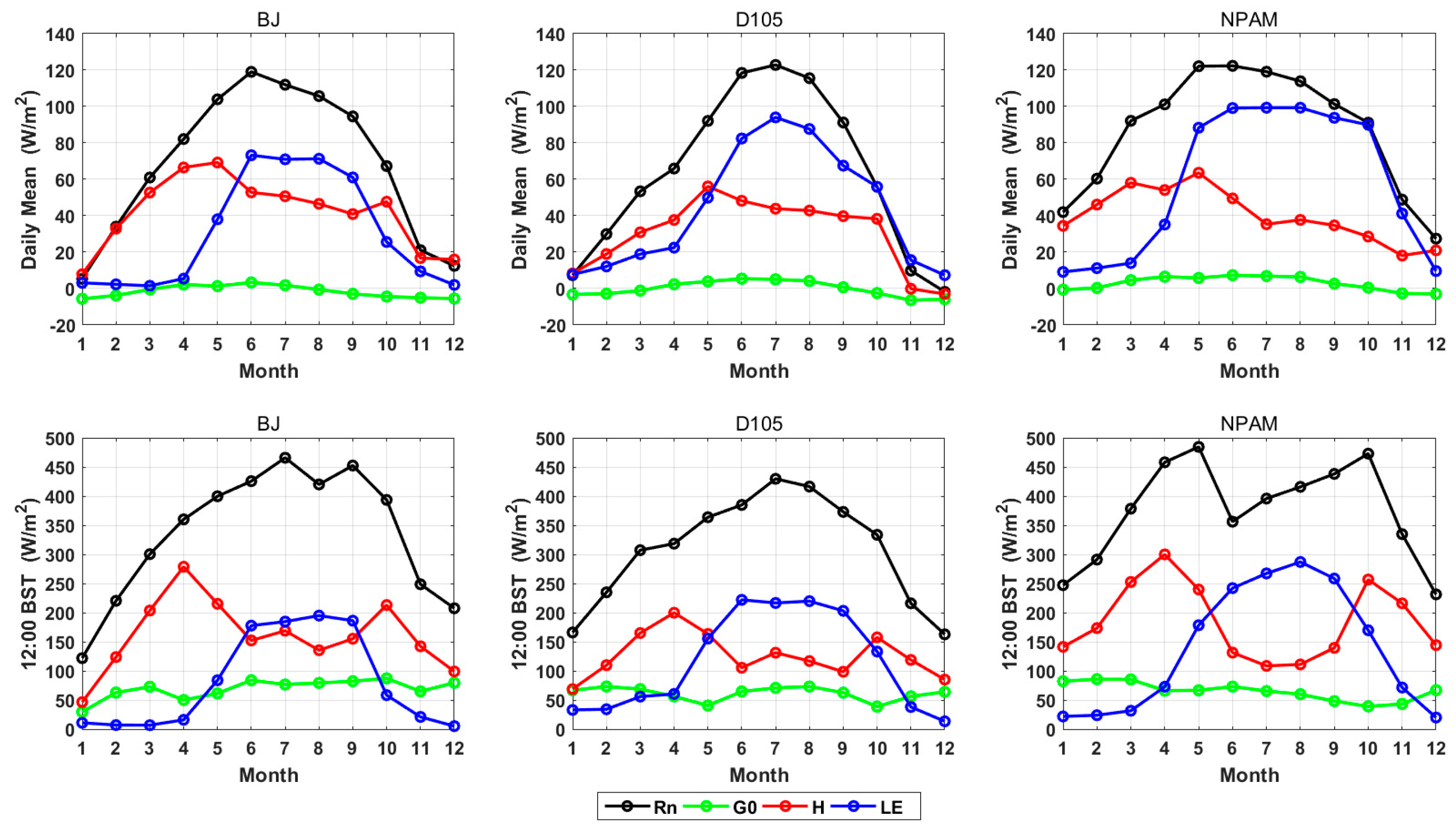
3.2. Multiple Timescale Variations in Land Surface Heat Fluxes

The monthly averaged diurnal variations in land surface heat fluxes at BJ, D105, and NPAM stations between January 2001 and December 2003 are shown in Figure 3a–c, respectively.
The land surface heat fluxes at these three stations exhibited distinct diurnal variations. The net radiation flux, soil heat flux, sensible heat flux, and latent heat flux generally reached their daily maxima at approximately 14:00 BST (12:00 local time). The sensible heat flux at night was generally negative because the surface temperature is generally lower than the near-surface air temperature; thus, the atmosphere heats the land surface. The latent heat flux remained positive throughout the day, indicating unidirectional water vapor transfer from the land surface to the atmosphere.
Of the land surface energy balance components, the soil heat flux value is the least important, while the sensible heat flux and latent heat flux are the two main components accounting for the net radiation flux, the value and significance of which vary seasonally. From January to April, the sensible heat flux is approximately one order of magnitude higher than the latent heat flux. In May, the latent heat flux increases rapidly. From June to September, based on the dominant latent heat of water vapor transfer, the latent heat flux is approximately two or three times higher than the sensible heat flux. In October, the latent heat flux decreases rapidly. From November to December, the sensible heat flux is dominant, similar to the situation from January to April.
Land surface heat fluxes over the northern Tibetan Plateau exhibit a drastic diurnal variability, which shows that the land surface is a very strong heat source in the daytime and is a weak heat sink at night [36]. The midday downward shortwave radiation is often observed to exceed 1200 W/m2 on cloudless days in summer [37]. Due to the thermodynamic effect, the extreme diurnal variability over the northern Tibetan Plateau may intensively influence the diurnal characteristics of the atmospheric boundary layer.
The monthly mean seasonal variations in land surface heat fluxes at the BJ, D105, and NPAM stations between January 2001 and December 2003 are shown in Figure 4, exhibiting both the daily means and values at 12:00 BST, which is closest to the overpass time of Landsat 7 over the northern Tibetan Plateau. The annual average values of the daily mean net radiation flux at BJ, D105, and NPAM were 68.1 W/m2, 63.3 W/m2, and 86.7 W/m2, and those of the soil heat flux were −1.8 W/m2, −0.2 W/m2, and 2.7 W/m2, respectively. The annual average values of the daily mean sensible heat flux at BJ, D105, and NPAM were 41.6 W/m2, 30.0 W/m2, and 40.0 W/m2, and those of the latent heat flux were 30.2 W/m2, 43.3 W/m2, and 57.4 W/m2, respectively.
In Figure 4, the daily means of sensible and latent heat flux were both positive throughout the year, even in the winter months. Thus, the surface heat densities were also positive in each month, and the northern Tibetan Plateau served as a heat source all year round. The daily mean sensible heat fluxes at BJ, D105, and NPAM stations all reached their maxima in May. The seasonal variations in land surface heat fluxes depict that land surface over the northern Tibetan Plateau is a strong heat source in summer and a weak heat source in winter.

3.3. Spatial Distributions of Land Surface Heat Fluxes

Satellite images from June 13, 2001, November 4, 2001, December 6, 2001, and May 15, 2002 were used as the representatives of summer, autumn, winter, and spring, respectively. The spatial distributions of net radiation flux, soil heat flux, sensible heat flux, and latent heat flux retrieved from satellite data on the four different dates are shown in Figure 5a–d, respectively.
The results showed that the land surface net radiation flux, soil heat flux, sensible heat flux, and latent heat flux all exhibited distinct seasonal variations. For a clear exhibition of the statistical distributions of the land surface heat fluxes above, their quartiles, Q1 (lower quartile), Q2 (median), and Q3 (upper quartile), which represent the 25%, 50%, and 75% positions in the value distribution, respectively, are listed in Table 5. The net radiation flux values changed numerically in the order summer > spring > autumn > winter, and their medians in those four seasons were 631.8 W/m2, 583.0 W/m2, 404.4 W/m2, and 314.3 W/m2, respectively. Compared with the net radiation flux, the soil heat flux exhibited a similar seasonal variation and was approximately an order of magnitude lower than the net radiation flux; the median soil heat flux values in summer, spring, autumn, and winter were 40.9 W/m2, 37.9 W/m2, 26.1 W/m2, and 20.5 W/m2, respectively. For the sensible heat flux, its seasonal variation was different and less prominent than that of the net radiation flux, and the median seasonal heat flux values in summer, spring, autumn, and winter were 252.7 W/m2, 219.5 W/m2, 221.4 W/m2, and 204.8 W/m2, respectively. Unlike the relatively mild seasonal change in the sensible heat flux, the seasonal variation in the latent heat flux was drastic, but also followed the order summer > spring > autumn > winter. The median latent heat flux values in the four seasons above were 320.1 W/m2, 298.3 W/m2, 142.3 W/m2, and 75.5 W/m2, respectively. The latent heat flux was higher than the sensible heat flux in summer and spring, and the situation was reversed in autumn and winter, which is consistent with the ground-based results discussed in Section 3.2.
The northeastern and western areas of these images were the relatively high- and low-value zones for fractional vegetation cover, respectively. Over the surfaces of lakes, rivers, and other water bodies, the sensible heat flux was lower than that of the surrounding land surface; the opposite was true of the latent heat flux. In addition to water bodies, areas with low sensible heat flux values and high latent heat flux values were distributed mainly in the northeast of these images throughout the four seasons; these areas basically corresponded to areas with high fractional vegetation cover values. Meanwhile, areas with high sensible heat flux values generally corresponded to areas with low latent heat flux values. Briefly, the sensible heat flux and the latent heat flux basically exhibited opposite and complementary characteristics in their spatial distributions.
Compared to those of the sensible heat flux and the latent heat flux, the spatial distribution of the net radiation flux was more homogenous and relatively less affected by the complex underlying surface. However, it can also be seen that the values of the net radiation flux in the northeast of these images in spring, summer, and autumn were slightly higher than those in the west. The soil heat flux was also affected by seasons, and its value in summer was slightly higher than that in winter.
The northern Tibetan Plateau basically has the characteristics of ideal natural underlying surfaces. Due to the complicated land cover types and complex topography over the northern Tibetan Plateau, land surface heat fluxes vary greatly over the heterogeneous landscape. Distribution of land surface heat fluxes with high spatial resolution from satellite images may enhance our understanding of the regional landscape and their impacts on the atmospheric circulations and climate change.

4. Discussion

In previous studies, estimates of 100–1000 km scale land surface heat fluxes distributions have been given much more attention than land–atmosphere interactions at 10–100 km regional scales. AVHRR, MODIS, and FY-2C/SVISSR have been widely used in the estimation of land surface heat fluxes on the Tibetan Plateau [10,14,16,18]. Land–atmospheric flux data derived from 10–100 m spatial resolution satellite products such as Landsat 7 ETM+ are essential and more suitable for estimating turbulent heat fluxes over regions at 10–100 km scales.
Additionally, from the 4 km resolution of FY-2C/SVISSR to the 1 km resolution of MODIS and the 60 m resolution of Landsat 7 ETM+, even for the same study area, satellite scenes at different spatial resolution will constitute a scene pyramid. The differences in satellite sensors and spatial resolutions could improve the quantitative analysis of land–atmosphere interactions over the same region.
In this paper, two different methods, CM and SEBS, were used for the estimation of land surface heat fluxes and then for comparison. In previous studies, the ground-based data applied were few and somewhat underused. For a more reliable assessment, the 3-year land surface heat flux timeseries derived from CAMP/Tibet in situ measurements were used for isochronic validation. Taking the CM calculations as ‘true values’, the results showed that the SEBS estimations were basically in accordance with the CM calculations. Compared with previous studies, the ground validation results had higher Pearson correlation coefficients. For a comprehensive analysis of land surface heat fluxes, the ground-based observation data used also emphasized the evaluation of their multiple timescale variation characteristics as a supplement.
In this paper, the midday land surface heat fluxes were estimated based on polar-orbiting satellite Landsat 7. For the estimation of land surface sensible heat flux and latent heat flux, the original errors of surface parameters and gradient observation data as well as the different calculation methods will produce some uncertainties. Due to the energy balance closure problem [38,39,40], where the net radiation flux is generally greater than the sum of the sensible heat flux, latent heat flux, and soil heat flux and the H deduction method with wet limit approximation used in the SEBS model for calculation of the latent heat flux, the estimated latent heat flux was higher than the in situ calculation, which may be one possible reason for the positive MB of the latent heat flux when comparing the satellite remote sensing data and in situ observations. The results of the negative MB of sensible heat flux and the positive MB of latent heat flux remain to be studied further. Additionally, the application of the NDVI also has some shortcomings such as the saturation of the NDVI over the surface with dense vegetation and uncertainties in some regions with a low vegetation fraction. The transformed NDVI or transformed squared NDVI might also overestimate or underestimate the fractional vegetation cover [41]. However, a recent study by Zou et al. [42] found that the land surface heat fluxes were less sensitive to NDVI than the temperature-related variables and wind speed (~0.4% changes in land surface temperature would cause ~11% changes in ET, while ~10% changes in NDVI would only cause ~0.2% changes in ET). Nevertheless, it is really a good suggestion for us to implement spectral mixture analysis methods in our future work to improve the accuracy of surface heat flux estimation.
Landsat 7 ETM+ satellite data have a high spatial resolution and are good for exhibiting the spatial distributions of sensible heat and latent heat flux; however, due to their limitations (long revisit intervals and low temporal resolution), it is difficult to accurately analyze their diurnal variations. Meanwhile, a large proportion of Landsat 7 images have relatively high mean cloudiness, which could result in considerable calculation errors in the estimation of land surface energy fluxes. Therefore, images with a mean cloudiness of over 40% were excluded in this paper for the sake of quality control of the satellite data; this criterion excluded the majority of Landsat 7 images. For the next step, future work may need to use geostationary satellite data to better reflect the spatial and temporal distributions of land surface heat fluxes.
Currently, a new generation of satellite sensors has come into service. The ECOSTRESS (ECOsystem Spaceborne Thermal Radiometer Experiment on Space Station) is designed to accurately measure the land surface temperature and evaporative stress index, which may substantially improve our understanding of energy and water transfer in the atmospheric boundary layer. Since the land surface temperature is one of the most important parameters in surface heat flux estimation and the evapotranspiration was estimated to be the most sensitive to land surface temperature [42], the potentially higher accuracy of land surface temperature measurement may further reduce the errors in energy flux retrievals. The Sentinel-3 is aimed at measurements of land surface temperature, sea surface temperature, sea surface topography, and sea surface color with high accuracy, which may be very useful for the comprehensive study of land–atmosphere and sea–atmosphere interactions. The GF-3 is the first C-band multi-polarization synthetic aperture radar imaging satellite with a resolution up to 1 m in China and is used for land observation and disaster monitoring under all-weather conditions. These up-to-date satellite data can be used for the accurate estimation of land surface heat fluxes.

5. Conclusions

Based on CAMP/Tibet in situ observation data and Landsat 7 ETM+ SLC-on data, land surface heat fluxes were calculated by the CM and the SEBS model. Their temporal variations and spatial distributions were clearly identified. The main conclusions are as follows:
(1) Four statistical indicators, RMSE, MB, MAE and R, were used to measure the degree of closeness of satellite remote sensing analysis and in situ calculations. For the net radiation flux, RMSE was 49.2 W/m2 and R was 0.957. For the soil heat flux, RMSE was 46.3 W/m2 and R was 0.645. For the sensible heat flux, RMSE was 68.2 W/m2 and R was 0.869. For the latent heat flux, RMSE was 54.9 W/m2 and R was 0.917. The result proves the effectiveness of land surface heat flux estimation based on the SEBS model. This algorithm may be further applied to a new generation of satellite sensors such as Sentinel-3, FY-4, and GF-3 in future work.
(2) The diurnal and seasonal variabilities of land surface heat fluxes depict the atmospheric boundary layer characteristics and the thermodynamic effect of the Tibetan Plateau, respectively. Land surface energy balance components generally reach their daily maxima at approximately 14:00 BST. The sensible heat flux at night is generally negative; thus, the atmosphere heats the land surface. The latent heat flux remains positive throughout the day, mirroring the unidirectional water vapor transfer from the land surface to the atmosphere. The annual average values of the daily mean net radiation flux at BJ, D105, and NPAM stations were 68.1 W/m2, 63.3 W/m2, and 86.7 W/m2, and those of the soil heat flux were −1.8 W/m2, −0.2 W/m2, and 2.7 W/m2, respectively. The annual average values of the daily mean sensible heat flux at BJ, D105, and NPAM stations were 41.6 W/m2, 30.0 W/m2, and 40.0 W/m2, and those of the latent heat flux were 30.2 W/m2, 43.3 W/m2, and 57.4 W/m2, respectively.
(3) Sensible heat flux and latent heat flux are two main components accounting for the net radiation flux, and vary seasonally. From November to April, the in situ sensible heat flux is higher than the latent heat flux. The opposite is the case between June and September, and May and October are transitional months. In summer, spring, autumn, and winter, the median values of the net radiation flux were 631.8 W/m2, 583.0 W/m2, 404.4 W/m2, and 314.3 W/m2, respectively; the soil heat flux was approximately an order of magnitude lower than the net radiation flux, and its median values were 40.9 W/m2, 37.9 W/m2, 26.1 W/m2, and 20.5 W/m2, respectively. For the sensible heat flux, its seasonal variation was less prominent than that of the net radiation flux, and the median values of the sensible heat flux were 252.7 W/m2, 219.5 W/m2, 221.4 W/m2, and 204.8 W/m2, respectively. The seasonal variation of latent heat flux was drastic, and its median values were 320.1 W/m2, 298.3 W/m2, 142.3 W/m2, and 75.5 W/m2, respectively. Apart from the sensible heat flux, the net radiation flux, soil heat flux, and latent heat flux all exhibited a trend of summer > spring > autumn > winter.
The spatio-temporal distributions of land surface heat fluxes may impact a broader scale understanding of the regional landscape. First, land surface heat fluxes over the northern Tibetan Plateau exhibit a drastic diurnal variability, which reveals that the land surface is a very strong heat source in the daytime and a weak heat sink at night. Second, the seasonal variations in land surface heat fluxes depict that land surface over the northern Tibetan Plateau is a strong heat source in summer and is a weak heat source in winter. Third, the northern Tibetan Plateau basically has the characteristics of ideal natural underlying surfaces. Due to the complicated land cover types and complex topography over the northern Tibetan Plateau, land surface heat fluxes vary greatly over the heterogeneous landscape. Additionally, due to the harsh environment of the Tibetan Plateau, the frequent extreme values of solar radiation (e.g., more than 1200 W/m2) may result in the anomalies of the turbulent heat fluxes, which will further have an impact on the regional and global atmospheric circulation and climate changes. From this point of view, more time series of satellite images, especially those images from geostationary satellites, would be of great help in the investigation of energy and water cycles over the Tibetan Plateau. In conclusion, the land surface processes over ‘The Third Pole’ will not only influence the local hydrometeorological environment, but also potentially serve as an indicator of global climate change.

Author Contributions

Conceptualization, L.Z., N.G., and Y.M.; Methodology, N.G.; Software, N.G., M.Z., and L.Z.; Validation, N.G., L.Z., and M.C.; Formal Analysis, N.G. and M.C.; Investigation, M.Z., Z.H., and X.W.; Resources, L.Z.; Data Curation, L.Z. and N.G.; Writing––Original Draft Preparation, N.G.; Writing––Review & Editing, L.Z. and Y.M.; Visualization, N.G. and M.Z.; Supervision, L.Z., N.G., and M.C.; Project Administration, L.Z.; Funding Acquisition, L.Z.

Funding

This research was jointly funded by the National Natural Science Foundation of China (Grant No. 41875031), the Strategic Priority Research Program of Chinese Academy of Sciences (Grant No. XDA20060101), the Chinese Academy of Sciences Basic Frontier Science Research Program from 0 to 1 Original Innovation Project (Grant ZDBS-LY-DQC005-01), the National Natural Science Foundation of China (Grant No. 41522501, 41275028, 41661144043), the Chinese Academy of Sciences (Grant No. QYZDJ-SSW-DQC019) and CLIMATE-TPE (ID 32070) in the framework of the ESA-MOST Dragon 4 Program.

Acknowledgments

The ITPCAS forcing data can be accessed from http://en.tpedatabase.cn/portal/MetaDataInfo.jsp?MetaDataId=202. The CAMP/Tibet data can be obtained from http://en.tpedatabase.cn/portal/MetaDataInfo.jsp?MetaDataId=217. The Landsat 7 ETM+ SLC-on data can be acquired from http://www.gscloud.cn/sources/list_dataset/242?cdataid=263&pdataid=10&datatype=L7slc-on#dlv=Wzg4LFswLDEwLDEsMF0sW1siZGF0YWRhdGUiLDBdXSxbXSw5OV0%3D. We thank two anonymous reviewers for their comments, which have helped us greatly improve the manuscript.

Conflicts of Interest

The authors declare no conflicts of interest.

References

  1. Foken. Micrometeorology, 1st ed.; Springer: Berlin/Heidelberg, Germany, 2008; pp. 8–23. [Google Scholar]
  2. Ullah, S.; Tahir, A.A.; Akbar, T.A.; Hassan, Q.K.; Dewan, A.; Khan, A.J.; Khan, M. Remote sensing-based quantification of the relationships between land use land cover changes and surface temperature over the lower Himalayan region. Sustainability 2019, 11, 5492. [Google Scholar] [CrossRef] [Green Version]
  3. Kato, S.; Yamaguchi, Y. Analysis of urban heat-island effect using ASTER and ETM+ data: Separation of anthropogenic heat discharge and natural heat radiation from sensible heat flux. Remote Sens. Environ. 2005, 99, 44–54. [Google Scholar] [CrossRef]
  4. Chakraborty, S.D.; Kant, Y.; Mitra, D. Assessment of land surface temperature and heat fluxes over Delhi using remote sensing data. J. Environ. Manag. 2015, 148, 143–152. [Google Scholar] [CrossRef]
  5. Ma, Y.; Tian, H.; Ishikawa, H.; Ohba, R.; Ueda, H.; Wen, J. Determination of regional land surface heat fluxes over a heterogeneous landscape of the Jiddah area of Saudi Arabia by using Landsat-7 ETM data. Hydrol. Process. 2006, 21, 1892–1900. [Google Scholar] [CrossRef]
  6. Zahira, S.; Abderrahmane, H.; Mederbal, K.; Frederic, D. Mapping latent heat flux in the western forest covered regions of Algeria using remote sensing data and a spatialized model. Remote Sens. 2009, 1, 795–817. [Google Scholar] [CrossRef] [Green Version]
  7. Carrasco-Benavides, M.; Ortega-Farías, S.; Lagos, L.O.; Kleissl, J.; Morales-Salinas, L.; Kilic, A. Parameterization of the satellite-based model (METRIC) for the estimation of instantaneous surface energy balance components over a drip-irrigated vineyard. Remote Sens. 2014, 6, 11342–11371. [Google Scholar] [CrossRef] [Green Version]
  8. Teixeira, A.H.C.; Padovani, C.R.; Andrade, R.G.; Leivas, J.F.; Victoria, D.D.C.; Galdino, S. Use of MODIS images to quantify the radiation and energy balances in the Brazilian Pantanal. Remote Sens. 2015, 7, 14597–14619. [Google Scholar] [CrossRef] [Green Version]
  9. Yang, Y.; Qiu, J.; Su, H.; Bai, Q.; Liu, S.; Li, L.; Yu, Y.; Huang, Y. A one-source approach for estimating land surface heat fluxes using remotely sensed land surface temperature. Remote Sens. 2017, 9, 43. [Google Scholar] [CrossRef] [Green Version]
  10. Ma, Y.; Su, Z.; Li, Z.; Koike, T.; Menenti, M. Determination of regional net radiation and soil heat flux over a heterogeneous landscape of the Tibetan Plateau. Hydrol. Process. 2002, 16, 2963–2971. [Google Scholar] [CrossRef]
  11. Ma, Y.; Zhong, L.; Su, Z.; Ishikawa, H.; Menenti, M.; Koike, T. Determination of regional distributions and seasonal variations of land surface heat fluxes from Landsat-7 Enhanced Thematic Mapper data over the central Tibetan Plateau area. J. Geophys. Res. Atmos. 2006, 111. [Google Scholar] [CrossRef] [Green Version]
  12. Oku, Y.; Ishikawa, H.; Su, Z. Estimation of land surface heat fluxes over the Tibetan Plateau using GMS data. J. Appl. Meteorol. Climatol. 2007, 46, 183–195. [Google Scholar] [CrossRef] [Green Version]
  13. Ma, W.; Ma, Y.; Li, M.; Hu, Z.; Zhong, L.; Su, Z.; Ishikawa, H.; Wang, J. Estimating surface fluxes over the north Tibetan Plateau area with ASTER imagery. Hydrol. Earth Syst. Sci. 2009, 13, 57–67. [Google Scholar] [CrossRef] [Green Version]
  14. Ma, Y.; Zhong, L.; Wang, B.; Ma, W.; Chen, X.; Li, M. Determination of land surface heat fluxes over heterogeneous landscape of the Tibetan Plateau by using the MODIS and in situ data. Atmos. Chem. Phys. 2011, 11, 10461–10469. [Google Scholar] [CrossRef] [Green Version]
  15. Chen, X.; Su, Z.; Ma, Y.; Yang, K.; Wang, B. Estimation of surface energy fluxes under complex terrain of Mt. Qomolangma over the Tibetan Plateau. Hydrol. Earth Syst. Sci. 2013, 17, 1607–1618. [Google Scholar] [CrossRef] [Green Version]
  16. Ma, Y.; Han, C.; Zhong, L.; Wang, B.; Zhu, Z.; Wang, Y.; Zhang, L.; Meng, C.; Xu, C.; Amatya, P. Using MODIS and AVHRR data to determine regional surface heating field and heat flux distributions over the heterogeneous landscape of the Tibetan Plateau. Theor. Appl. Climatol. 2014, 117, 643–652. [Google Scholar] [CrossRef] [Green Version]
  17. Han, C.; Ma, Y.; Chen, X.; Su, Z. Estimates of land surface heat fluxes of the Mt. Everest region over the Tibetan Plateau utilizing ASTER data. Atmos. Res. 2016, 168, 180–190. [Google Scholar] [CrossRef]
  18. Zhong, L.; Ma, Y.; Hu, Z.; Fu, Y.; Hu, Y.; Wang, X.; Cheng, M.; Ge, N. Estimation of hourly land surface heat fluxes over the Tibetan Plateau by the combined use of geostationary and polar-orbiting satellites. Atmos. Chem. Phys. 2019, 19, 5529–5541. [Google Scholar] [CrossRef] [Green Version]
  19. He, J.; Yang, K. China Meteorological Forcing Dataset; Cold and Arid Regions Science Data Center: Lanzhou, China, 2011. [Google Scholar] [CrossRef]
  20. Chen, Y.Y.; Yang, K.; He, J.; Qin, J.; Shi, J.C.; Du, J.Y.; He, Q. Improving land surface temperature modeling for dry land of China. J. Geophys. Res. 2011, 116, D20104. [Google Scholar] [CrossRef]
  21. Ma, Y.; Su, Z.; Koike, T.; Yao, T.; Ishikawa, H.; Ueno, K.; Menenti, M. On measuring and remote sensing surface energy partitioning over the Tibetan Plateau—From GAME/Tibet to CAMP/Tibet. Phys. Chem. Earth 2003, 28, 63–74. [Google Scholar] [CrossRef]
  22. Thom, A.S.; Stewart, J.B.; Oliver, H.R.; Gash, J.H.C. Comparison of aerodynamic and energy budget estimates of fluxes over a pine forest. Q. J. R. Meteorol. Soc. 1975, 101, 93–105. [Google Scholar] [CrossRef]
  23. Hu, Y.; Qi, Y. The combinatory method for determination of the turbulent fluxes and universal functions in the surface layer. J. Meteorol. Res. 1993, 7, 101–109. [Google Scholar]
  24. Zou, M.; Zhong, L.; Ma, Y.; Hu, Y.; Feng, L. Estimation of actual evapotranspiration in the Nagqu river basin of the Tibetan Plateau. Theor. Appl. Climatol. 2018, 132, 1039–1047. [Google Scholar] [CrossRef]
  25. Su, Z. The Surface Energy Balance System (SEBS) for estimation of turbulent heat fluxes. Hydrol. Earth Syst. Sci. 2002, 6, 85–100. [Google Scholar] [CrossRef]
  26. Foken, T. 50 years of the Monin-Obukhov Similarity Theory. Bound. Layer Meteorol. 2006, 119, 431–447. [Google Scholar] [CrossRef]
  27. Brutsaert, W. On a derivable formula for long-wave radiation from clear skies. Water Resour. Res. 1975, 11, 742–744. [Google Scholar] [CrossRef]
  28. Kumar, L.; Skidmore, A.K.; Knowles, E. Modelling topographic variation in solar radiation in a GIS environment. Int. J. Geogr. Inf. Sci. 1997, 11, 475–497. [Google Scholar] [CrossRef]
  29. Yang, K.; He, J.; Tang, W.J.; Qin, J.; Cheng, C.C.K. On downward shortwave and longwave radiations over high altitude regions: Observation and modeling in the Tibetan Plateau. Agric. For. Meteorol. 2010, 150, 38–46. [Google Scholar] [CrossRef]
  30. Dhungel, R.; Allen, R.G.; Trezza, R.; Robison, C.W. Comparison of latent heat flux using aerodynamic methods and using the Penman-Monteith method with satellite-based surface energy balance. Remote Sens. 2014, 6, 8844–8877. [Google Scholar] [CrossRef] [Green Version]
  31. Daughtry, C.S.T.; Kustas, W.P.; Moran, M.S.; Pinter, P.J., Jr.; Jackson, R.D.; Brown, P.W.; Nichols, W.D.; Gay, L.W. Spectral estimates of net radiation and soil heat flux. Remote Sens. Environ. 1990, 32, 111–124. [Google Scholar] [CrossRef]
  32. Gao, Z.Q.; Liu, C.S.; Gao, W.; Chang, N.B. A coupled remote sensing and the Surface Energy Balance with Topography Algorithm (SEBTA) to estimate actual evapotranspiration over heterogeneous terrain. Hydrol. Earth Syst. Sci. 2011, 15, 119–139. [Google Scholar] [CrossRef] [Green Version]
  33. Brutsaert, W. Aspects of bulk atmospheric boundary layer similarity under free-convective conditions. Rev. Geophys. 1999, 37, 439–451. [Google Scholar] [CrossRef]
  34. Yang, K.; Koike, T.; Fujii, H.; Tamagawa, K.; Hirose, N. Improvement of surface flux parametrizations with a turbulence-related length. Q. J. R. Meteorol. Soc. 2002, 128, 2073–2087. [Google Scholar] [CrossRef]
  35. Faivre, R.; Colin, J.; Menenti, M. Evaluation of methods for aerodynamic roughness length retrieval from very high-resolution imaging LIDAR observations over the Heihe basin in China. Remote Sens. 2017, 9, 63. [Google Scholar] [CrossRef] [Green Version]
  36. Ma, Y.; Wang, Y.; Wu, R.; Hu, Z.; Yang, K.; Li, M.; Ma, W.; Zhong, L.; Sun, F.; Chen, X.; et al. Recent advances on the study of atmosphere-land interaction observations on the Tibetan Plateau. Hydrol. Earth Syst. Sci. 2009, 13, 1103–1111. [Google Scholar] [CrossRef] [Green Version]
  37. Ma, Y.; Fan, S.; Ishikawa, H.; Tsukamoto, O.; Yao, T.; Koike, T.; Zuo, H.; Hu, Z.; Su, Z. Diurnal and inter-monthly variation of land surface heat fluxes over the central Tibetan Plateau area. Theor. Appl. Climatol. 2005, 80, 259–273. [Google Scholar] [CrossRef]
  38. Foken, T. The energy balance closure problem: An overview. Ecol. Appl. 2008, 18, 1351–1367. [Google Scholar] [CrossRef]
  39. Zhong, L.; Ma, Y.; Su, Z.; Lu, L.; Ma, W.; Lu, Y. Land-atmosphere energy transfer and surface boundary layer characteristics in the Rongbu Valley on the northern slope of Mt. Everest. Arct. Antarct. Alp. Res. 2009, 41, 396–405. [Google Scholar] [CrossRef] [Green Version]
  40. Leuning, R.; Gorsel, E.V.; Massman, W.J.; Isaac, P.R. Reflections on the surface energy imbalance problem. Agric. For. Meteorol. 2012, 156, 65–74. [Google Scholar] [CrossRef]
  41. Sousa, D.; Small, C. Spectral Mixture Analysis as a unified framework for the remote sensing of evapotranspiration. Remote Sens. 2018, 10, 1961. [Google Scholar] [CrossRef] [Green Version]
  42. Zou, M.; Zhong, L.; Ma, Y.; Hu, Y.; Huang, Z.; Xu, K.; Feng, L. Comparison of two satellite-based evapotranspiration models of the Nagqu River Basin of the Tibetan Plateau. J. Geophys. Res. Atmos. 2018, 123, 3961–3975. [Google Scholar] [CrossRef]
Figure 1. (a) Elevation variation (units: m) of the study area (the CAMP/Tibet (Coordinated Enhanced Observing Period (CEOP) Asia–Australia Monsoon Project on the Tibetan Plateau) area is marked by the red rectangular border) and (b) fractional vegetation cover distribution estimated from Landsat 7 ETM+ data on June 13, 2001 (Path 138/Row 038) over the northern Tibetan Plateau.
Remotesensing 11 02899 g001
Figure 2. Comparison of surface heat fluxes estimated by the SEBS model with those calculated by the CM: (a) net radiation flux, (b) soil heat flux, (c) sensible heat flux, and (d) latent heat flux.
Remotesensing 11 02899 g002
Figure 3. Monthly averaged diurnal variations of land surface net radiation flux, soil heat flux, sensible heat flux, and latent heat flux at (a) BJ, (b) D105, and (c) NPAM station from January 2001 to December 2003.
Remotesensing 11 02899 g003
Figure 4. Averaged seasonal variations of land surface net radiation flux, soil heat flux, sensible heat flux, and latent heat flux at BJ, D105, and NPAM stations from January 2001 to December 2003 (daily mean and 12:00 BST).
Remotesensing 11 02899 g004
Figure 5. Spatial distribution of net radiation flux Rn, soil heat flux G0, sensible heat flux H, and latent heat flux LE: (a) 13/06/2001, (b) 04/11/2001, (c) 06/12/2001, and (d) 15/05/2002.
Remotesensing 11 02899 g005
Table 1. Ground Measurement Stations in the Study Area.
StationLongitude (°E)Latitude (°N)Altitude (m)Underlying Land Cover Type
ANNI92.1724431.254424480Alpine and subalpine meadow
BJ91.8987131.368664509Alpine and subalpine meadow
D10591.9425633.064295039Alpine and subalpine plain grass
NPAM91.7146831.926234620Alpine and subalpine meadow
Table 2. Information of several meteorological elements measured at automatic weather stations. (Note: for wind speed, air temperature, relative humidity, soil temperature, and soil heat flux, the instruments were placed at multiple levels. The heights (or depths for z < 0) of each level for each meteorological element are listed in this table. Two sensors are placed at z = 0 cm to measure soil surface temperature).
Meteorological ElementsLevelsLevel HeightsTemporal ResolutionAccuracyInstruments
Wind speed3z = 10 m, 5 m, 1 m1 h0.1 m/sWS-D32 (Komatsu)
Air temperature2z = 8.2 m, 1 m1 h0.05 KTS-801/Pt100 (Okazaki)
Air pressure1z = 0.5 m1 h0.5 hPaPTB220C (Vaisala)
Relative humidity2z = 8.2 m, 1 m1 h2%HMP-45D (Vaisala)
Radiation budgets1z = 1.28 m1 h5%CM21 (Kipp&Zonen) (for shortwave), PIR (Kipp&Zonen) (for longwave)
Soil temperature6z = 0 cm, 0 cm, −4 cm, −10 cm, −20 cm, −40 cm1 h0.2 KTS-301/Pt100 (Okazaki)
Soil heat flux2z = −10 cm, −20 cm1 h2%MF-81 (EKO)
Table 3. Information of Landsat 7 ETM+ Images Used in this Work.
ScenePath/RowDate (dd/mm/yyyy)Overpass Time
1137/03813/11/200104:11 UTC
2137/03816/11/200204:10 UTC
3137/03803/01/200304:11 UTC
4137/03804/02/200304:11 UTC
5137/03824/03/200304:11 UTC
6138/03713/06/200104:18 UTC
7138/03715/05/200204:17 UTC
8138/03813/06/200104:18 UTC
9138/03804/11/200104:17 UTC
10138/03806/12/200104:17 UTC
11138/03815/05/200204:17 UTC
12138/03822/10/200204:16 UTC
13138/03816/04/200304:17 UTC
Table 4. Band List of Landsat 7 ETM+.
ChannelBandWavelength Range (μm)Spatial Resolution (m)
1Blue0.45–0.5230
2Green0.52–0.6030
3Red0.63–0.6930
4Near infrared0.76–0.9030
5Shortwave infrared1.55–1.7530
6Thermal infrared10.4–12.560
7Shortwave infrared2.08–2.3530
8Panchromatic0.5–0.915
Table 5. Quartiles of land surface heat fluxes estimated by satellite data (units: W/m2).
Date13/06/200104/11/200106/12/200115/05/2002Mean
Net radiation fluxQ1566.4357.8271.5514.8427.6
Q2631.8404.4314.3583.0483.4
Q3704.2451.6359.4668.5545.9
Soil heat fluxQ136.722.917.633.527.7
Q240.926.120.537.931.3
Q345.729.423.643.535.5
Sensible heat fluxQ1176.4130.3147.6161.6154.0
Q2252.7221.4204.8219.5224.6
Q3341.9302.8257.4289.9298.0
Latent heat fluxQ1195.261.32.8204.3115.9
Q2320.1142.375.5298.3209.1
Q3443.7223.2139.1413.9305.0

