Abstract
In this paper, we propose a novel strategy to estimate the micro-motion (m-m) of ships from synthetic aperture radar (SAR) images. To this end, observe that the problem of motion and m-m detection of targets is usually solved using synthetic aperture radar (SAR) along-track interferometry through two radars spatially separated by a baseline along the azimuth direction. The approach proposed in this paper for m-m estimation of ships, occupying thousands of pixels, processes the information generated during the coregistration of several re-synthesized time-domain and not overlapped Doppler sub-apertures. Specifically, the SAR products are generated by splitting the raw data according to a temporally small baseline using one single wide-band staring spotlight (ST) SAR image. The predominant vibrational modes of different ships are then estimated. The performance analysis is conducted on one ST SAR image recorded by COSMO-SkyMed satellite system. Finally, the newly proposed approach paves the way for application to the surveillance of land-based industry activities.
1. Introduction
Synthetic aperture radar (SAR) provides high-resolution images of static ground scenes, whereas processing of data containing ground object motion results in a variation of focused areas. A special case of such motion is vibration where its pattern may be distinctly identifiable in focused SAR intensity images, as well as in a precise amplitude analysis. The X-band SAR can be well suited to image vibration because its wavelength is close to typical vibration amplitudes. This work extends the investigation technique observed in [1] where the pixel tracking has been used for the first time to detect small movements of marine targets. Before this work, several interesting research studies have been performed in the field of micro-motion (m-m) estimation. In [2] the effects of rotation and vibration in millimeter-waveforms have been assessed by processing simulated and real SAR data. Vibrating targets cause the modulation of the azimuth phase history of a SAR image. This phenomenon may be considered as a micro-Doppler (m-D) frequency modulation. In [3] the oscillation frequency and amplitude were computed from the time-frequency distributions and the findings were in accordance with the respective ground truths. In [4] a vibrating m-D signature for a bistatic SAR system with a fixed receiver was analyzed and compared to the signature obtained in a monostatic SAR system. The derived model was useful for m-D classification and suitable to perform target recognition. The derived model has been verified on simulated data at 94 GHz and 10 GHz. In [5], the authors implemented a wavelet approach to perform a m-m analysis for inverse SAR (ISAR) systems. Feature extraction was successfully applied to SAR data collected by military and civilian radars. In [6], the generalized likelihood ratio test (GLRT) was devised to detect target m-m. The performance was investigated using both simulated and quasi-real data, showing the effectiveness of the GLRT under low signal-to-noise/clutter ratios. Sometimes the m-D effect may significantly decrease the readability of the ISAR and SAR images. In [7], the authors successfully designed a method to remove these effects, exploiting the spectrogram and complex time-frequency analysis of raw data. In [8] the model for vibrating targets in multiple input multiple output (MIMO) SAR was derived. Numerical examples verified the influence of vibration parameters on imaging and time-frequency profile and showed that the same target exhibits different m-D signatures in different MIMO channels. The authors also highlight the potential of MIMO SAR for 3D m-m estimation. In [9,10,11,12] different strategies for ships and ship wake detection were consolidated using compressed sensing and convex-programming approaches. Several methods were implemented in [13,14,15] for Earth displacement estimation by tracking only the magnitude of single-look-complex (SLC) couples of interferometric SAR images. This procedure is evaluated in the course of the coregistration process where the azimuth and range shifts are used to build-up a two-dimensional displacement map. In this paper, we exploit this method to estimate the m-D of maritime targets using several temporal sub-apertures of a single CSK staring spotlight (ST) SAR image. Illustrative examples, obtained on real recorded data, show the effectiveness of the proposed technique in estimating the vibrational fingerprint of the maritime vessels. Remarkably, these results pave the way for the application of the proposed technique to the surveillance of land-based industry facilities.
The remainder of this paper is organized as follows. The details of the estimation procedure are described in Section 2. This section is comprised of Section 2.1 which describes the concepts of the computational model, Section 2.2 presenting the technique used to estimate the coregistration shifts, and Section 2.3 wherein the architecture designed to estimate the m-m is described from a computational point of view. Section 3 contains numerical examples based upon two real study-cases. The last section concludes the paper and introduces future research tracks.
2. Estimation Procedure and Processing Architecture
This section consists of three parts aimed at guiding the reader towards the design of the estimation procedure. More precisely, the first part provides a description of the underlying vibrational model from the physical point of view, whereas the second part explains the ideas behind the estimation procedure. Finally, the third part presents the entire processing chain and describes each operation performed in the course of the parameter estimation.
2.1. Computational Model
In this subsection, we present the model used to describe the vibrations generated by a ship. Since the whole ship can be considered as a complex body consisting of several interacting mechanical components, the analysis of its behavior represents a formidable task. For this reason, at the design stage, the vibration analysis is carried out by resorting to finite element techniques. In fact, a common practice consists in first dividing the ship into five parts:
- Hull beam (keel);
- Main structural substructures;
- Local structural elements.
- On-board equipment (electrical power facilities);
- Main propulsion systems.
Then, the vibration contribution of each of these components are analyzed. The forces involved along the 3-dimensional reference system can be seen in Figure 1a. The forces (F1, F2, F3) are generated by the rotation movement of the propulsion propeller, amplified by the sail effect generated by the rudder. The forces (F4, F5) are instead due to the movement of the main axis of the transmission of motion generated by the machines. The coupling system and the engine revolutions-per-minute (rpm) reduction box generates the force F6 while the diesel engine will pull the forces (F7, F8). These are the main sources of vibration, generated by a ship, that propagate along all the structures and superstructures that make up the hull. Figure 1b represents the same ship observed in SAR coordinates. The point P1 is hit by the electromagnetic pulses and, during the image formation process, is projected on the point P2 located on the layover projection plane constituting the SAR image. If P1 vibrates along the three Euclidean dimensions, P2 exhibits a vibration in the range-azimuth SAR plane located into the new vector-space slant coordinates. Standard SAR-processing methods are based upon the assumption of a static scene. If targets are moving, their positions in the SAR-image are shifted in azimuth and range-azimuth plan and a defocusing may occur. Figure 2 shows the SAR acquisition geometry of the target P1 having a displacement of velocity with respect to the sensor. According to Figure 2 the azimuth SAR resolution is determined by the SAR aperture length L, the electromagnetic wavelength and the angle between the velocity vector and line of sight :
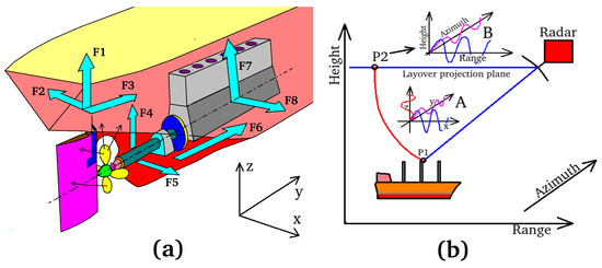
Figure 1.
Forces generated by a ship. (a) General scheme observed in the 3D space. (b) Representation into the range-azimuth SAR slant coordinates.
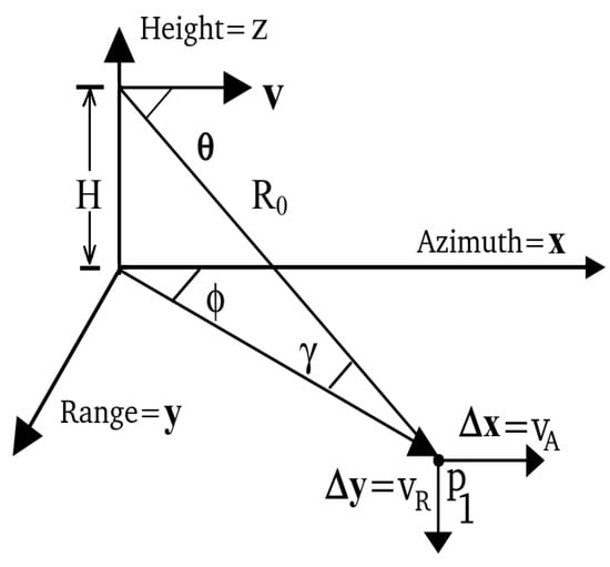
Figure 2.
Geometric model of the SAR acquisition.
The Doppler frequency shift of the stationary target is given by:
where is the platform velocity and is the angle existing between the velocity vector and the target direction located at distance . On the other hand, the Doppler shift defines the azimuth position in the SAR image located on the following angle:
If the target P1 has a velocity component along the range direction, it exhibits the following Doppler shift:
In the course of the focusing process, this frequency error is transformed into an angular error denoted by . Let us consider the differential version of (2)
and equal this variation to (4), then the differential of is given by:
This parameter produces an azimuth target miss-location due to a range velocity component with respect to the radar platform. The Doppler phase variation from a point reflector can be observed through the output of the matched filter whose expression is:
where is the range variation due to the SAR antenna motion along its aperture. According to Figure 2, if the sensor is flying following the path and the target is moving along where and with , it is possible to approximate the relative range variation by that of a stationary reflector modified by a correction term due to the target movement. If , then
Replacing x and y with the respective expressions in (8) and neglecting the higher order terms, can be expressed as:
where
and
The target velocity components of (12) introduce an azimuth displacement as described by (6). The velocities and accelerations, , in Formula (13), represent the contribution of the target to global acceleration and provide the variation of the Doppler frequency in the received signal. This result can be viewed as a smearing effect along azimuth and polarized in the same direction as the target’s speed. Thus, the existence of nonzero target speeds and accelerations leads to a quality degradation of the image contrast since the signal to clutter ratio decreases. This degradation effect is quantified through the following equation:
According to (7), where , the corresponding phase error returns a defocusing and the reduction of the target contrast in the SAR image. The resulting frequency is given by the phase derivative and covers the following bandwidth over the time interval :
Now, from the differentiation of (2), and imposing that , the azimuth resolution of the moving target becomes . Using Equation (1), we obtain:
By combining (16) and (14), the degraded azimuth resolution of moving targets can be estimated. The blurring significantly increases for fine-resolution mapping and highly squinted angles of observation. There is also a range resolution decrease due to the target range migration during the time of measurement. In the case of a non-accelerating target, the parameter is dominant and according to and Formulas (16) and (1) yields:
Recalling that the , the target defocusing can be expressed as:
which relates the defocusing length to the movement of the target during the time of measurement. Summarizing, moving targets produce significant position errors in the azimuth positioning due to the target range velocity component. Moreover, it leads to smearing effects on the focused signals in both range and cross-range directions. A pure displacement along the azimuth direction returns a pure defocusing along the same direction. All these effects are detected by two-dimensional normalized cross-correlation and tracked during the staring spotlight orbital time by the sub-pixel coregistration process. In the next subsection, this process is explained in detail.
2.2. Estimation Procedure
Sub-pixel offset tracking (SPOT) is a relevant technique to measure large-scale ground displacements in both range and azimuth directions. The technique is complementary to differential interferometric SAR and persistent scatterers interferometry when the radar phase information is unstable [16,17]. In this paper, we apply the above pixel tracking technique to a single spotlight image instead of multi-temporal interferometric images. Specifically, the single observation is divided into Doppler sub-apertures in order to investigate the fastest displacements of moving targets. Note that the acquisition duration is of the order of a few hundredths of a second.
With the above remarks in mind, we focus on maritime applications and estimate the displacement generated by the marine targets detected using a single SAR image focused in Doppler sub-apertures. In accordance with the temporal subdivision strategy of Figure 3, we observe the offset trend by computing the normalized cross-correlation once the image is partitioned into small patches. The estimation procedure consists in shifting the master for each temporal event and calculating the correlation between adjacent Doppler sub-apertures, according to a small-temporal baseline strategy. In order to provide a more operational approach to the technique we used the software Sarproz, implemented by Prof. D. Perissin. The software is versatile because it provides the use of parallel computing and allows the possibility of designing all the coregistration parameters.
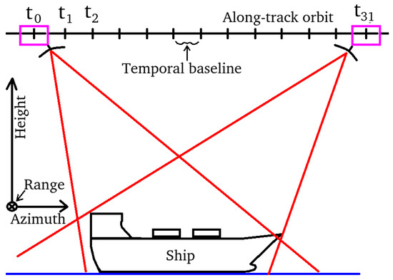
Figure 3.
SAR geometry of the small multi-temporal baseline strategy.
For the proposed estimation procedure, we set the cross-correlation window size to pixels and the oversampling factor to 64 in both the range and azimuth directions. All the coregistration parameters are reported in Table 2. The offset components of the sub-pixel normalized cross-correlation, according to [18,19] are described by the complex parameter which is estimated by the following equation:
Specifically, in (19) is the offset component (18) generated by the earth displacement; is the offset component generated by the earth displacement when located on highly sloped terrain; is the offset caused by residual errors of the satellite orbits; is the offset component generated by general attitude and control errors of the flying satellite trajectory; and are the contributions generated by the electromagnetic aberrations due to atmosphere parameters, space and time variations, and general disturbances due to thermal and quantization noise, respectively. The atmospheric time-variation during the very short acquisition time interval has little influence on the temporal component of the last displacement parameters because of its low accuracy. All errors are compensated for by choosing only high energy and stable points and subtracting the initial offsets in order to retrieve the shift contributions only generated by the target displacement.
As the concluding remark of this subsection, we note that the limits of the proposed procedure are mainly due to the maximum frequency of vibration observed and the minimum sensitivity in sensing vibration amplitudes. The first parameter is directly related to the sampling frequency. In fact, it is equal to the sampling frequency divided by two. For the specific case considered in the next section, 200 sub-apertures are produced over an acquisition time of 12 s. If we refer to this configuration, the time baseline is equal to 0.06 s. Thus, the maximum observation frequency is approximately 33 Hz, this means that it is possible to observe the vibrations generated by an endothermic engine running at 33–60 rpm. As for the minimum sensitivity, it is directly related to the spatial resolution of the sensor. In respect of the specific sensor used to assess the procedure, namely the SAR sensor of a CSK satellite, the spatial resolution is approximately one meter. In order to finalize a precise coregistration, we choose an over-sampling factor equal to 200. This value, in principle, allows dividing the single pixel range-azimuth into sub-pixels and, thanks to this, the minimum estimated displacement was equal to five millimeters.
2.3. Computational Architecture Description
In this subsection, we describe in detail the processing chain used to perform the estimation of m-m. To this end, the block-scheme of the architecture is shown in Figure 4a. The input of the processing architecture is a single raw dataset (block 1). The computational block 2 consists of a temporal n-stage splitter that is responsible for generating n temporal sub-apertures. In the numerical examples, we generate 200 sub-products. The duration of the full-band Doppler Spotlight acquisition is about 12 s. This means that the observation time increment between two contiguous sub-apertures is approximately 0.06 s. The aim of block 3 is to focus all the n sub-apertures. The final results are a time series of SAR images in the SLC configuration having lower resolution in azimuth. This resolution loss is inversely proportional to the lost Doppler band fraction. Note that SAR products generated by block 3 are not yet coregistered, this operation is implemented in block 5, which performs the sub-pixel coregistration whose setting parameters are generated by block 4. Specifically, the SAR acquisition characteristics summary and the coregistration settings are shown in Table 1 and Table 2 respectively. Moreover, the master of the multiple coregistration processes is selected according to the strategy referred to in the following as “small-temporal baseline” with the sliding master. The output of the co-recorder is represented by block 6. The result is a stack of maps of shifts in range and azimuth. Now, blocks 7 and 8 perform pixel by pixel analysis to estimate the oscillations of the ships. Figure 4b represents a more detailed explanation of computational blocks 7 and 8. The input of block 7 consists of a single column of shifts, that for the case at hand, has a dimensionality of . The vector of shifts is complex and after the coregistration process the displacements are estimated along both the range and azimuth direction. The computational block 7.1 interpolates the input data by a given factor. Next, block 7.2 carries out the operation of fast Fourier transform (FFT) in order to evaluate the oscillation modes on the slant coordinates identified by the pixel of the original image focused in the full band. Finally, block 8 performs the m-m extrapolation and is composed by a bank of bandpass filters in order to extrapolate the oscillations in the time domain. This block returns and which describe the m-m in the time and frequency domain, respectively. The nature of the time-domain displacement estimable using this technique is extended along the SAR range and azimuth dimensions. The vibrations observed predominantly are those in the low frequencies, compatible with those generated by the endothermic engines used for the production of the on-board electrical energy.
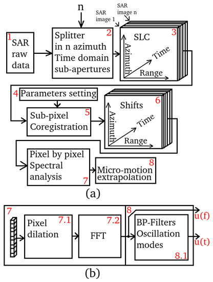
Figure 4.
Computational architecture scheme. (a) General scheme. (b) Detailed scheme concerning computational blocks 7 and 8.

Table 1.
SAR acquisition characteristics summary.
Table 2.
Coregistration parameters.
3. Experimental Results
In this section, we provide some experimental results by analyzing the vibrational modes of two ships at anchor. Moreover, we analyze in depth the frequency response and the trend over the time of the vibrations by selecting seven measurement points for the first study case and two measurement points for the second one. All points are distributed widely on the outer deck of the ships. The results also include the estimation of the distribution of the resonance frequencies distributed in the space where a comparative analysis of two vibration profiles extracted both along the keel and along the ship’s deck is also carried out. Detailed information about the processed SAR image are summarized in Table 3.
Table 3.
SAR observation parameters.
3.1. Study Case 1
Figure 3 shows the spotlight SAR acquisition geometry. The SAR observation takes about 12 s using approximately 25 kHz of the Doppler band. The whole image formation history was divided into 200 temporal azimuth sub-apertures of duration about s, according to a small temporal baselines strategy. Figure 5 is a schematic representation of the parameters estimated by the coregistration procedure. The square number one is a focused pixel of the master image and the square number two is the same pixel but located on the slave image. The parameters d and are the distance between the master and slave pixel centers and the angle respect to the horizontal axis respectively. Figure 6a depicts the magnitude of the ROI of the ship under test. Figure 6b represents the estimated vibration energy, consisting in parameter d of Figure 5 integrated through time. Figure 7a shows the average phase spanned in time of the pixel displacement. This parameter consists of the angle indicated in Figure 5, whereas Figure 7b contains the measurement points map of the ship.
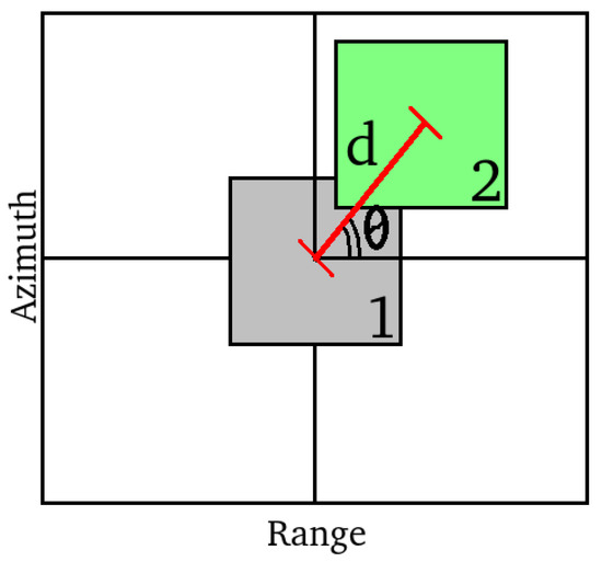
Figure 5.
Schematic representation of isolated pixels with a certain shift due to space displacement.
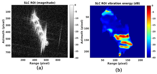
Figure 6.
(a) SLC of the ROI under test. (b) Vibration field (magnitude).
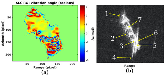
Figure 7.
(a) Vibration field (phase). (b) Points of measurement representation.
It is important to observe that the estimation of slow-rate variation velocities is performed using the SAR investigation technique called along-track interferometry (ATI). Unfortunately, this configuration requires the use of two or more radars separated by an along-track-baseline of variable length from a few meters up to a few tens of meters. The longer the baseline, the greater the sensitivity of the Doppler variations of this bistatic SAR system. It is clear that in order to obtain a high sensitivity to vibrations, it is necessary to design high baselines ATI geometries. However, there are no satellite systems configured in this way and therefore it is necessary to find other solutions [1]. Decomposing the raw SAR data into multiple Doppler sub-apertures may not be a fully successful solution. This is because investigating the raw data generated by Earth observation satellites, which are usually never oversampled [1], will never be possible to estimate correlated ATI interferograms. In fact, in Figure 8a,b the module and phase of infra-chromatic coherence are visible. Inspection of the figures confirms that no information can be extrapolated. Another technique to estimate the m-m consists in evaluating the anomalies of the Doppler centroid during the focusing stage. This technique is also not immune to problems because a reliable estimation might occur if raw SAR images are available. However, such data are not always easy to obtain at this level of processing. Moreover, this solution is suitable for estimating vibrations only in the azimuth dimension. The proposed technique allows the estimation of the displacements, even if of lower intensity, in both range and azimuth directions, thanks to the highly accurate estimation of the shifts made by the co-registrator. As stated before, we consider seven measurement points and for each of them the vibration spectrum and the temporal trend of movements in the time domain are displayed in Figure 9, Figure 10, Figure 11, Figure 12, Figure 13, Figure 14 and Figure 15. The location of each point is summarized in Table 4.
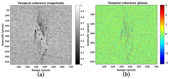
Figure 8.
(a): Intra-chromatic coherence (magnitude). (b): Intra-chromatic coherence (phase).
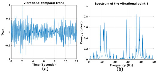
Figure 9.
(a) Measurement point number 1 temporal trend. (b) Measurement point number 1 frequency spectrum.
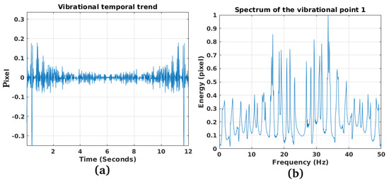
Figure 10.
(a) Measurement point number 2 temporal trend. (b) Measurement point number 2 frequency spectrum.
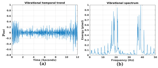
Figure 11.
(a) Measurement point number 3 temporal trend. (b) Measurement point number 3 frequency spectrum.
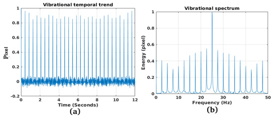
Figure 12.
(a) Measurement point number 4 temporal trend. (b) Measurement point number 4 frequency spectrum.
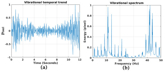
Figure 13.
(a) Measurement point number 5 temporal trend. (b) Measurement point number 5 frequency spectrum.
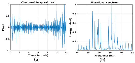
Figure 14.
(a) Measurement point number 6 temporal trend. (b) Measurement point number 6 frequency spectrum.
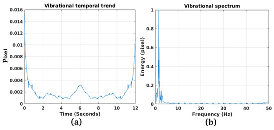
Figure 15.
(a) Measurement point number 7 temporal trend. (b) Measurement point number 7 frequency spectrum.
Table 4.
Case of study 1—Measurement points list.
Figure 9a represents the trend over the time of the vibrations existing at measurement point number 1 and having intensity approximately over 0.45. The amplitude of the vibrations are of a medium entity in fact, as shown by Figure 6b, at this point coincides average energy equal to –5 dB. The vibrational modes, shown in Figure 9b, are very intense with the maximum localized at about 37 Hz. The results for measurement point number 2 are shown in Figure 10a,b. Figure 10a shows the trend of displacements over time. In this case, the amplitude of oscillation is rather low compared to the previous case with the maximum equal to 0.2. Figure 10b shows the vibrational frequency spectrum. In this case, the spectral lines are well defined with a maximum at about 34 Hz. The results for measurement point number 3 are shown in Figure 11a,b. Figure 11a shows the trend of displacements over time. On this measurement point, the amplitude of oscillation is also lower with respect to vibrations observed on the measurement point 1 where an average value is located to 0.25 starting from 2 s to approximately 11 s. Figure 11b shows the vibrational frequency spectrum. In this case, the spectral lines are well defined with a maximum around 23 Hz and 36 Hz. The measurement point number 4 is the most particular because it is chosen to study the vibrations present at the end of the front master of the ship. As Figure 12a shows, the oscillations over time have numerous peaks at the maximum amplitude of 1 unit. The preponderance of these peaks is very stable at 25 Hz, as shown by Figure 12b, which represents the spectrum. The results concerning the time domain vibration pattern of measurement points 5 and 6 are reported in Figure 13a and Figure 14a, respectively. The figures show a similarity with mean values around 0.4. The corresponding spectra are shown in Figure 13b and Figure 14b, confirming resonance oscillations of about 12 and 42 Hz for point 5 and 32 Hz at measurement point 6. No significant oscillations are measured at this point. Figure 15a shows the time course of the displacement observed on the measurement point number 7 for which negligible amplitude values are measured (on average about 0.0030 compared to the maximum of 1 unit). The spectrum has a very low maximum frequency, located around 2 Hz (result showed in Figure 15b). A global view of the resonance frequencies distributed over all the pixels composing the ship is shown in Figure 16. The figure shows two reflectivity profiles marked with the numbers 1 and 2. The first reflectivity profile is shown in Figure 17a. This orientation was chosen in order to study the trend of keel vibrations. This representation in amplitude is given by the plus markers while the frequency value is represented by times markers. It is considered very important to underline that both physical values have been normalized to 1 so as to show the trend on the same graph. Finally, Figure 17b represents the trend of the resonance frequency (plus points) due to the vibration energy (times symbols). The observations are measured along with the vibrational profile 2. It is found that an increase in frequency corresponds to an increase in vibration energy, both on the keel (profile number 1) and on the transverse profile (profile number 2).
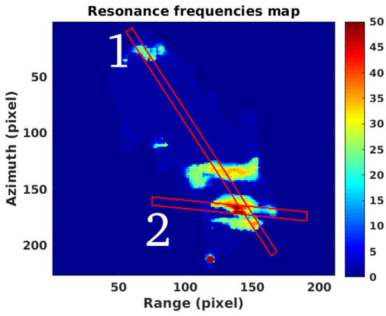
Figure 16.
Vibrational profiles selected for results discussion.
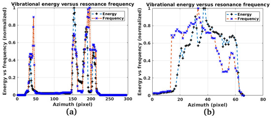
Figure 17.
Vibrations observed along the profiles selected in Figure 16. (a) Vibrational profile 1. (b) Vibrational profile 2.
3.2. Study Case 2
In this second case, the object under investigation is a merchant ship specially chosen with many lateral lobes and disturbances due to defocusing effects that are markedly more visible in the Doppler domain. This worst case allows us to test the robustness of the estimation algorithm. Figure 18 is the SLC in magnitude of the ship. The optical image of the vessel concerning the second case study is contained in Figure 19a. The considered measurement points are two as summarized in Table 5.
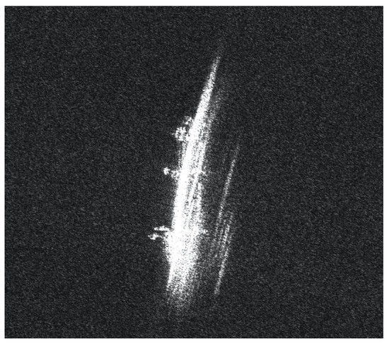
Figure 18.
SLC SAR of the study-case number two.
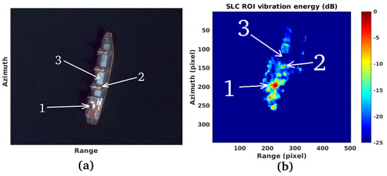
Figure 19.
Study case number two results. (a): Optical image. (b): Vibrational map.
Table 5.
Case of study 2—Measurement points list.
Figure 19b represents the energy map of vibrations where a high energy level can be observed at the measurement point 1 and coinciding with the chimney stack. This structure clearly vibrates more than the rest of the ship and this anomaly is correctly detected. Figure 20a,b represents the time-domain trend and spectrum of vibrations present on measurement point 1 where the predominant modes of vibration in the form of spectral lines are very visible. Some predominant frequencies are detected at approximately 14 and 36 Hz. Figure 21a,b represents the time-domain trend and spectrum of vibrations present on measurement point 2. Also in this case the predominant modes of vibration in the form of spectral lines are very visible. Some predominant frequencies are detected at approximately 13 and 38 Hz.
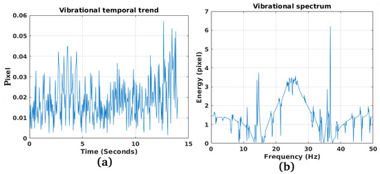
Figure 20.
Study case number two results. (a): Temporal vibrational trend on the measurement point 1. (b): Spectrum of the vibrational trend on the measurement point 1.
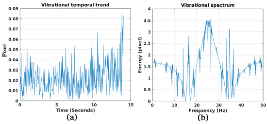
Figure 21.
Study case number two results. (a): Temporal vibrational trend on the measurement point 2. (b): Spectrum of the vibrational trend on the measurement point 2.
4. Discussion and Future Assessments
The results obtained in this work have proved that the use of amplitude information alone from SAR Spotlight images is enough to estimate the m-m generated by ships. As a matter of fact, the exploitation of high-resolution SAR Spotlight data has allowed us to obtain displacement maps with millimetric precision and, hence, to appreciate the m-m. The vibrations have been estimated in the time and frequency domain considering two different ships. In the first domain, an analysis from the energy point of view can be performed, while in the second domain the main oscillation modes can be identified at frequencies ranging from a few Hz to a few tens of Hz. More importantly, it is very likely that the observed oscillation modes are due to the machines used to generate the electrical energy on board, namely generated by the diesel alternators. As a matter of fact, the propulsion system of large ships can be generally designed following two ways. In the first case, the propeller is connected directly to the endothermic engine. This is a case which is usually adopted on oil tankers, equipped with very large and slow engines. The resulting frequencies are very low, quantifiable at no more than 10 Hz. The other approach consists in installing a speed reducer between the diesel endothermic engine and the propeller shaft. This solution is widely used because it allows the engine to run at higher rates with respect to the rotation frequency of the propeller shaft. The resulting frequencies will necessarily be higher with respect to the previous situation and varying from approximately 10 to few tens of Hz. Thus, considering the estimated results, we are confident about the reliability of the estimation algorithms and we have observed ships belonging to the second category.
In addition, given the high quality of the vibration profiles, we believe that this work opens the way to the design of high-performance ship detection, classification, and recognition methods. For instance, the vibrational map of coded targets allows establishment of whether or not the ship engines are turned on, or to locate the position of the engine room within the naval silhouette. Moreover, in principle, it could be also possible to recognize the number and type of engines installed on board through the deep-learning approach. Finally, the herein developed approach can be further extended to estimate the vibrations generated by terrestrial industrial installations, coal-fired, and nuclear power plants.
5. Materials and Methods
In this section, we describe the software tools and the hardware used in the performance analysis in order to provide the detailed guidelines for the replication of the experiments. Specifically, the authors used a laptop equipped with am Intel core i7 and 16 GB RAM. The considered software to estimate the coregistration shifts is SARPROZ: https://www.sarproz.com/. Finally, MATLAB scripts have been created by the authors to generate the Doppler sub-apertures.
Author Contributions
Conceptualization, F.B., C.C., P.A. and D.O.; methodology, F.B., C.C., P.A. and D.O.; software, F.B.; validation, F.B., C.C., P.A. and D.O.; formal analysis, F.B., C.C., P.A. and D.O.; investigation, F.B., C.C., P.A. and D.O.; resources, F.B. data curation, F.B.; writing—original draft preparation, F.B., C.C., P.A. and D.O.; writing—review and editing, F.B., C.C., P.A. and D.O.; visualization, F.B., C.C., P.A. and D.O.; supervision, D.O.; project administration, F.B.; funding acquisition, F.B.
Funding
This research received no external funding.
Conflicts of Interest
The authors declare no conflict of interest. The authors whose names are listed immediately below the title certify that they have no affiliations with or involvement in any organization or entity with any financial interest (such as honoraria; educational grants; participation in speakers’ bureaus; membership, employment, consultancies, stock ownership, or other equity interest; and expert testimony or patent-licensing arrangements), or non-financial interest (such as personal or professional relationships, affiliations, knowledge or beliefs) in the subject matter or materials discussed in this manuscript. No founders are involved during the designation and the life of this project.
Abbreviations
The following abbreviations are used in this manuscript:
| SS | Staring Spotlight |
| m-m | micro-motion |
| ROI | Region of Interest |
| MTI | Moving Target Indicator |
| LRSD | Low-Rank plus Sparse Decomposition |
| RT | Radon transform |
| MIMO | Multiple Input Multiple Output |
| SPOT | Pixel Offset Tracking |
| GLRT | Generalized Likelihood Ratio Test |
| LOS | Line of Sight |
| ERS | European remote sensing satellite system |
| CSK | COSMO-SkyMed |
| ATI | Along-Track-Interferometry |
| SAR | Synthetic Aperture Radar |
| ISAR | Interferometric SAR |
| DEM | Digital Elevation Model |
| FFT | Fast Fourier Transform |
| SLC | Single Look Complex |
| BP-Filter | Band Pass Filter |
References
- Filippo, B. COSMO-SkyMed Staring Spotlight SAR Data for Micro-Motion and Inclination Angle Estimation of Ships by Pixel Tracking and Convex Optimization. Remote Sens. 2019, 11, 766. [Google Scholar] [CrossRef]
- Ruegg, M.; Meier, E.; Nuesch, D. Vibration and rotation in millimeter-wave SAR. IEEE Trans. Geosci. Remote Sens. 2007, 45, 293–304. [Google Scholar] [CrossRef]
- Sparr, T.; Krane, B. Micro-Doppler analysis of vibrating targets in SAR. IEE Proc.-Radar Sonar Navig. 2003, 150, 277–283. [Google Scholar] [CrossRef]
- Clemente, C.; Soraghan, J.J. Vibrating target micro-Doppler signature in bistatic SAR with a fixed receiver. IEEE Trans. Geosci. Remote Sens. 2012, 50, 3219–3227. [Google Scholar] [CrossRef]
- Thayaparan, T.; Suresh, P.; Qian, S.; Venkataramaniah, K.; SivaSankaraSai, S.; Sridharan, K.S. Micro-Doppler analysis of a rotating target in synthetic aperture radar. IET Signal Process. 2010, 4, 245–255. [Google Scholar] [CrossRef]
- Deng, B.; Wang, H.Q.; Li, X.; Qin, Y.L.; Wang, J.T. Generalised likelihood ratio test detector for micro-motion targets in synthetic aperture radar raw signals. IET Radar Sonar Navig. 2011, 5, 528–535. [Google Scholar] [CrossRef]
- Stankovic, L.; Thayaparan, T.; Dakovic, M.; Popovic-Bugarin, V. Micro-Doppler removal in the radar imaging analysis. IEEE Trans. Aerosp. Electron. Syst. 2013, 49, 1234–1250. [Google Scholar] [CrossRef]
- Zhao, G.; Fu, Y.; Nie, L.; Zhuang, Z. Imaging and micro-Doppler analysis of vibrating target in multi-input?multi-output synthetic aperture radar. IET Radar Sonar Navig. 2015, 9, 1360–1365. [Google Scholar] [CrossRef]
- Bandiera, F.; Orlando, D.; Ricci, G. On the CFAR property of GLRT-based direction detectors. IEEE Trans. Signal Process. 2007, 55, 4312–4315. [Google Scholar] [CrossRef]
- Biondi, F. Low rank plus sparse decomposition of synthetic aperture radar data for maritime surveillance. In Proceedings of the 2016 4th International Workshop on Compressed Sensing Theory and its Applications to Radar, Sonar and Remote Sensing (CoSeRa), Aachen, Germany, 19–22 September 2016; pp. 75–79. [Google Scholar]
- Biondi, F. Low-rank plus sparse decomposition and localized radon transform for ship-wake detection in synthetic aperture radar images. IEEE Geosci. Remote Sens. Lett. 2018, 15, 117–121. [Google Scholar] [CrossRef]
- Biondi, F. A Polarimetric Extension of Low-Rank Plus Sparse Decomposition and Radon Transform for Ship Wake Detection in Synthetic Aperture Radar Images. IEEE Geosci. Remote Sens. Lett. 2019, 16, 75–79. [Google Scholar] [CrossRef]
- Casu, F.; Manconi, A.; Pepe, A.; Lanari, R. Deformation time-series generation in areas characterized by large displacement dynamics: The SAR amplitude pixel-offset SBAS technique. IEEE Trans. Geosci. Remote Sens. 2011, 49, 2752–2763. [Google Scholar] [CrossRef]
- Scambos, T.A.; Dutkiewicz, M.J.; Wilson, J.C.; Bindschadler, R.A. Application of image cross-correlation to the measurement of glacier velocity using satellite image data. Remote Sens. Environ. 1992, 42, 177–186. [Google Scholar] [CrossRef]
- Giles, A.B.; Massom, R.A.; Warner, R.C. A method for sub-pixel scale feature-tracking using Radarsat images applied to the Mertz Glacier Tongue, East Antarctica. Remote Sens. Environ. 2009, 113, 1691–1699. [Google Scholar] [CrossRef]
- Wang, Z.; Perissin, D.; Lin, H. Subway tunnels identification through Cosmo-SkyMed PSInSAR analysis in Shanghai. In Proceedings of the 2011 IEEE International Geoscience and Remote Sensing Symposium, Vancouver, BC, Canada, 24–29 July 2011. [Google Scholar]
- Perissin, D.; Wang, T. Repeat-pass SAR interferometry with partially coherent targets. IEEE Trans. Geosci. Remote Sens. 2012, 50, 271–280. [Google Scholar] [CrossRef]
- Nitti, D.O.; Hanssen, R.F.; Refice, A.; Bovenga, F.; Nutricato, R. Impact of DEM-assisted coregistration on high-resolution SAR interferometry. IEEE Trans. Geosci. Remote Sens. 2011, 49, 1127–1143. [Google Scholar] [CrossRef]
- Biondi, F.; Clemente, C.; Orlando, D. An atmospheric phase screen estimation strategy based on multi-chromatic analysis for differential interferometric synthetic aperture radar. IEEE Trans. Geosci. Remote Sens. 2019, 1–12. [Google Scholar] [CrossRef]
© 2019 by the authors. Licensee MDPI, Basel, Switzerland. This article is an open access article distributed under the terms and conditions of the Creative Commons Attribution (CC BY) license (http://creativecommons.org/licenses/by/4.0/).