Regional Vicarious Calibration of the SWIR-Based Atmospheric Correction Approach for MODIS-Aqua Measurements of Highly Turbid Inland Water

Abstract

Water color remote sensing requires accurate atmospheric correction but this remains a significant challenge in highly turbid waters. In this respect, the shortwave infrared (SWIR) band-based atmospheric correction approach has proven advantageous when applied to the moderate resolution imaging spectroradiometer (MODIS) onboard the Aqua satellite. However, even so, uncertainties affect its accuracy. We performed a regional vicarious calibration of the MODIS-Aqua SWIR (1240, 2130)-based atmospheric correction using in situ water surface reflectance data measured during different seasons in Lake Taihu, a highly turbid lake. We then verified the accuracy of the (1240, 2130)-based atmospheric correction approach using these results; good results were obtained for the remote sensing reflectance retrievals at the 555, 645, and 859 nm, with average relative errors of 15%, 14%, and 22%, respectively, and no significant bias. Comparisons with the (1240, 2130)-based iterative approach and (1640, 2130)-based approach showed that the vicarious calibrated (1240, 2130)-based approach has the best accuracy and robustness. Thus, it is applicable to the highly turbid Lake Taihu. It may also be applicable to other highly turbid inland waters with similar optical and aerosol optical properties above water, but such applications will require further validation.

1. Introduction

Water color satellite sensors receive top-of-atmosphere (TOA) radiance, which includes water-leaving and atmospheric path radiance. Water-leaving radiance, which can be used to assess water parameters, must be derived from satellite-received TOA radiance [1]. This process is known as atmospheric correction, which is the basis for water color remote sensing. Gordon and Wang [1] proposed an atmospheric correction approach (abbreviated as GW94) based on the “black near-infrared (NIR) water-leaving radiance” assumption. This approach uses two NIR bands to assess aerosol radiance and then interpolates the aerosol radiance to visible (VIS) bands. Previous studies have applied this approach to the sea-viewing wide field-of-view sensor (SeaWiFS) and the moderate-resolution imaging spectroradiometer (MODIS), which have all yielded good results in open ocean waters [2]. For turbid coastal and inland waters, however, the near-infrared water-leaving radiance is apparently greater than zero and, therefore, the “black NIR” assumption is no longer valid. Therefore, the GW94 approach fails to perform accurate atmospheric correction in turbid water. Using the “black NIR”-based approach, studies have developed a number of improved methods for turbid waters, which include two main categories. The first attempts to develop models to assess the water-leaving radiance in NIR bands mainly using an iterative approach [3,4,5,6,7]. The second approach uses atmospheric information derived from adjacent clear water and interpolates the corrections to the turbid water [8]. These improved approaches usually work well in moderately turbid waters but are not necessarily valid for highly turbid waters since certain waters saturate the NIR bands, rendering these “black NIR”-based approaches completely unusable.

Wang and Shi [9,10,11] proposed a “black shortwave infrared (SWIR)”-based approach, which assumes that the water-leaving radiance in the SWIR bands is zero and uses two SWIR bands to replace the two NIR bands present in the original GW94 approach. Due to the strong absorption at the SWIR wavelengths from pure water [12], the water-leaving radiance in the SWIR wavelength for even highly turbid water tends to be zero. Therefore, the SWIR-based atmospheric correction approach can be used for highly turbid waters. Previous studies have already verified this approach with its application to MODIS-Aqua data in several areas with highly turbid water, including the East China Sea and eastern coast of the U.S.A. [9,10,13,14]. These studies used two SWIR bands at 1240 and 2130 nm because 14 out of the 20 detectors for the original 500 m resolution 1640 nm band on the MODIS-Aqua are inoperable. However, in certain highly turbid waters, such as areas in Lake Taihu, we cannot neglect the water-leaving radiance at the 1240 nm band and the original (1240, 2130) SWIR-based atmospheric correction approach will overestimate aerosol scattering and underestimate the water-leaving radiance in the visible and NIR bands. To solve this problem, Wang et al. [15] proposed an iterative approach and used the relatively clear water pixels at the center of Lake Taihu to retrieve an aerosol model from the original (1240, 2130) SWIR band-based atmospheric correction and interpolated the aerosol model to the entire lake. With the interpolated aerosol model and the 2130 nm band determined aerosol scattering, they then performed atmospheric correction for the entire lake. Zhang et al. [16] suggested that the center of Lake Taihu is not always relatively clear and, therefore, revised the iterative approach by selecting the 200 pixels with the clearest water in the entire lake, as opposed to only the middle area of the lake. However, there are still several uncertainties in the (1240, 2130)-based iterative method. Lake Taihu is a large lake, with an area of over 2300 km², surrounded by large metropolitan areas, such as Suzhou, Wuxi, Changzhou, and Huzhou. Therefore, aerosol models applicable above the entire lake may significantly change in certain circumstances. Otherwise, locating relatively clear water in Lake Taihu is not always easy, which leads to the failure of the (1240, 2130)-based iterative method. To avoid these uncertainties, Wang et al. [17] replaced the 1240 nm band with the 1640 nm band and applied the (1640, 2130)-based atmospheric correction approach because the water-leaving radiance at 1640 nm is more likely to be near zero due to higher water absorption at longer wavelengths. However, since 70% of the detectors for the original 500 m resolution 1640 nm band on the MODIS-Aqua are inoperable, the (1640, 2130)-based method cannot be applied operationally.

Except for the uncertainties mentioned above, there are a number of other uncertainties associated with the atmospheric correction of water color remote sensing images. To improve the accuracy of atmospheric correction, previous studies have widely adopted vicarious calibration as an operational method [18,19,20,21,22,23,24,25]. Vicarious calibration uses the in situ-measured water-leaving radiance coincident with the water color remote sensing images to compute the vicarious calibration coefficients, i.e., the gains, to obtain the original TOA radiance of the water color remote sensing images. Vicarious calibration can cancel out the error sources and uncertainties in the atmospheric correction process, thus improving atmospheric correction accuracy. For open ocean waters, studies have performed reliable vicarious calibrations based on the in situ water-leaving radiance measured by the marine optical buoy (MOBY) [20,26]. The vicarious calibration coefficients for MODIS-Aqua have been previously applied to the operational processing of MODIS-Aqua data. However, these calibration coefficients are applicable to clear open ocean waters when using the NIR-based atmospheric correction approach but may not be suitable for highly turbid waters when using the SWIR-based atmospheric correction approach. Therefore, to improve the accuracy of the SWIR-based atmospheric correction approach in highly turbid waters, we recommend the vicarious calibration of the SWIR-based atmospheric correction approach for highly turbid waters. In this study, we performed regional vicarious calibration of MODIS-Aqua data over highly turbid waters using the SWIR-based atmospheric correction approach. We used in situ water surface reflectance data measured in the highly turbid Lake Taihu during different seasons to perform the vicarious calibration of the (1240, 2130)-based atmospheric correction approach. We then verified the accuracy of the (1240, 2130)-based atmospheric correction approach with the vicarious calibrated results.

2. Study Area and Data Description

2.1. Study Area Description

Lake Taihu in eastern China was selected as the study area (Figure 1). It is the third largest freshwater lake in China and has an area of over 2300 km² [27]. Lake Taihu is a highly turbid lake, with an average concentration of total suspended matter that is greater than 50 mg L⁻¹ and a maximum concentration of total suspended matter that is greater than 300 mg L⁻¹ [28]. Taihu Lake is located in the core area of the middle and lower reaches of the Yangtze River, and is the source of drinking for surrounding cities such as Wuxi and Suzhou. In recent years, the water properties of Lake Taihu have attracted significant attention for remote sensing data studies [16,17,28,29,30,31,32,33,34,35,36,37].

From 2005 to 2014, we performed 12 cruise surveys of Lake Taihu, during which we measured the in situ water surface reflectance at 377 water sampling stations, whose locations are shown in Figure 1.

Table 1. The dates and sampling stations for each cruise survey performed on Lake Taihu.

Cruise Dates	Number of Stations	Cruise Dates	Number of Stations
Oct. 10, 2005	13	Mar. 14–15, 2009	29
Jan. 7–9, 2006	47	Apr. 17–27, 2009	51
Jul. 29 to Aug. 1, 2006	39	Oct. 17–18, 2012	9
Oct. 12–15, 2006	37	May 11–13, 2013	40
Jan. 7–9, 2007	50	Jul. 21–22, 2014	8
Apr. 25–27, 2007	40	Oct. 26, 2014	14

lists relevant information, such as the dates and sampling stations, for each cruise survey.

2.2. Water Surface Reflectance Measurements

During the 12 cruise surveys, we measured the in situ water surface reflectance spectra at each sampling station with an ASD portable field spectrometer FieldSpec® Pro VNIR (wavelength range from 350–1,000 nm) and FieldSpec® Pro FR (wavelength range from 350–2,500 nm) using the above water method [38]. At each station, we measured the standard panel (L_p(λ)), water (L_sw(λ)), and skylight (L_sky(λ)) on the open deck. With these measurements, we calculated the remote sensing reflectance (R_rs(λ)) with the following equation:

$$R_{rs}\left(\lambda \right)=\frac{L_w\left(\lambda \right)}{E_d\left(\lambda \right)}=\frac{L_{sw}\left(\lambda \right)-r_{sky}{L}_{sky}\left(\lambda \right)}{\pi L_p\left(\lambda \right)/{\rho }_p\left(\lambda \right)}$$

(1)

where λ is wavelength, E_d(λ) is the downward irradiance above the water surface, L_w(λ) is the water-leaving radiance, ρ_p(λ) is the reflectance of the standard panel calibrated in the laboratory, and r_sky is the skylight reflectance at the air–water interface, which can be determined from the look-up table [39]. Wind speeds at each sampling station were measured simultaneously with reflectance measurements and were used to determine r_sky values.

Figure 2 shows the calculated R_rs spectra for the 12 cruise surveys. Previous studies have already applied several of these R_rs data to study the water properties of Lake Taihu [24,29,40,41,42].

2.3. MODIS-Aqua Description

MODIS, an onboard Aqua satellite, was launched on 4 May, 2002. Of the 36 bands equipped on MODIS, 16 can be used to study water properties, including nine 1 km spatial resolution ocean color bands (i.e., 412, 443, 488, 531, 547, 667, 678, 748, and 869 nm), five 500 m land bands (i.e., 469, 555, 1240, 1640, and 2130 nm), and two 250 m bands (645 and 859 nm). For highly turbid waters, out of the nine ocean color bands, six bands (547, 667, 678, 748, and 869 nm) often become saturated and should not be used. The three SWIR bands (i.e., 1240, 1640, and 2130 nm) can be used for atmospheric corrections. Finally, the eight other visible and NIR bands (i.e., 412, 443, 469, 488, 531, 555, 645, and 859 nm) can be used to study the water properties of highly turbid waters. Out of these eight bands, the four land bands (i.e., 469, 555, 645, and 859 nm) have both higher spatial resolution and radiometric dynamic range and are, therefore, more beneficial when studying the water properties of highly turbid coastal and inland waters, because highly turbid waters produce higher reflectance signals than clear waters. In this study, we analyzed the atmospheric correction result accuracy of these eight bands (i.e., 412, 443, 469, 488, 531, 555, 645, and 859 nm), with a primary focus on the four land bands (i.e., 469, 555, 645, and 859 nm).

We used coincident in situ remote sensing reflectance data to calibrate and verify the atmospheric correction results of the MODIS-Aqua data, which include 18 scenes of images referred to as: A20060080540, A20060090445, A20062100440, A20062110520, A20062120425, A20070070430, A20070080510, A20070090555, A20071160535, A20090730540, A20091070530, A20091120545, A20091160520, A20122910440, A20122920525, A20131320535, A20142020430, and A20142990510.

3. Methods

3.1. Regional Vicarious Calibration Method

The water–air radiometric transfer function [20] is given by the following equation:

L_t(λ) = (t_dv(λ)L_w(λ) + L_a(λ) + L_r(λ) + tL_f(λ) + TL_g(λ))t_gs(λ)t_gv(λ)f_p(λ)

(2)

where L_t(λ), L_a(λ), L_r(λ), tL_f(λ), and TL_g(λ) are the TOA radiance, aerosol scattering radiance, which includes Rayleigh–aerosol interactions, Rayleigh scattering radiance (air molecule scattering), surface whitecap radiance, and sunglint, respectively; t_dv(λ) is the water surface to satellite diffuse transmittance; t_gv(λ) and t_gs(λ) are the gaseous absorption from the water surface to the sensor and Sun to water surface, respectively; and f_p(λ), is the correction coefficient for the band sensor response to the observed radiance polarization.

Vicarious calibration is based on this water–air radiometric transfer function, which uses the coincidently in situ-measured R_rs(λ) to model L_t(λ), followed by regression analysis with the corresponding MODIS-received L_t(λ). Before input into Equation (2), the in situ-measured R_rs(λ) should be transformed to L_w(λ) as follows [43]:

L_w(λ) = nL_w(λ)(f_scos(θ_s)t_ds(λ)f_b(λ)) =(R_rs(λ)*F₀(λ))(f_scos(θ_s)t_ds(λ)f_b(λ))

(3)

where nL_w(λ) is the normalized water-leaving radiance, F₀ is the TOA solar irradiance at the average Earth–Sun distance, f_s is the adjustment parameter for changes in the Earth–Sun distance, θ_s is the solar zenith angle, t_ds(λ) is the Sun to water surface diffuse transmittance, and f_b(λ) is the water surface bidirectional reflectance correction parameter.

The parameters in Equations (2) and (3) can be computed using the SeaWiFS data analysis system (SeaDAS 7.2) based on the SWIR (1240, 2130 nm) atmospheric correction approach. We computed L_w(λ) by inputting the coincidently in situ-measured R_rs(λ) into Equation (3) and then calculated L_t(λ) by inputting the computed L_w(λ) into Equation (2). We further use the computed L_t(λ) and its corresponding MODIS-received L_t(λ) to perform regression analysis, as shown in Equation (4). We then obtained the vicarious calibration coefficients for each band. We note that this regression equation only contains gain (λ) but no offset (λ) because this is a more stable technique [20].

L_t^Computed(λ) = gain(λ) * L_t^MODIS(λ)

(4)

The in situ R_rs(λ) spectra data should be convolved into R_rs(λ_i) with the relative spectral response function for each MODIS-Aqua VIS-NIR band before substitution into Equation (3):

$$R_{rs}({\lambda }_i)=\frac{{\displaystyle {\int }_{{\lambda }_{\min }}^{{\lambda }_{\max }}{R}_{rs}\left(\lambda \right)f_{\mathrm{i}}\left(\lambda \right)d\lambda }}{{\displaystyle {\int }_{{\lambda }_{\min }}^{{\lambda }_{\max }}{f}_i\left(\lambda \right)d\lambda }}$$

(5)

where f_i(λ) is the relative spectral response function for each MODIS-Aqua band and λ_min and λ_max are the wavelength range of the spectral response function for each band.

We note that the coincident in situ R_rs(λ) or nL_w(λ) spectra are key parameters in the vicarious calibration process. Vicarious calibration of the NIR-based atmospheric correction approach often uses the in situ nL_w(λ) spectra measured by the marine optical buoy (MOBY) in clear oceanic waters off Hawaii [20]. Vicarious calibration of the SWIR-based atmospheric correction approach can also use MOBY data, which is beneficial for the NIR-SWIR combined atmospheric correction algorithm [23]. However, MOBY data will also yield larger uncertainties due to the low signal-to-noise ratio that characterizes the SWIR bands over clear oceanic waters. Although we are attempting to improve the SWIR-based atmospheric correction accuracy over highly turbid inland waters, such as Lake Taihu, we do not need to consider the combination with the NIR-based atmospheric correction algorithm. Therefore, to reduce uncertainty caused by the low signal-to-noise ratio, we instead used in situ R_rs(λ) data from the highly turbid Lake Taihu for the vicarious calibration of the SWIR-based atmospheric correction approach. The vicarious calibration results can also counteract local aerosol effects and yield improved accuracy at Lake Taihu, as well as similar adjacent lakes that are highly turbid.

3.2. Atmospheric Correction Based on Vicarious Calibration Results

After we obtained the vicarious calibration coefficients for the eight MODIS-AQUA VIS-NIR bands, we substituted them into the SeaDAS7.2 to perform the SWIR-based atmospheric corrections. In the SeaDAS7.2 l2gen module, we input the vicarious calibration coefficients for the eight VIS-NIR bands into the “gain” parameters. We note that the “gain” parameters should include 16 numbers for all 16 bands that can be used for water optical property studies, whereas we used the default numbers provided in the SeaDAS7.2 as the “gain” parameters for the other 8 bands.

Table 2. The SeaWiFS data analysis system (SeaDAS)7.2 parameter settings for atmospheric correction based on the shortwave infrared (SWIR) (1240, 2130) combined with the vicarious calibration results. The gain(412), gain(443), gain(469), gain(488), gain(531), gain(555), gain(645), and gain(859) should be replaced with the vicarious calibration results. The other numbers in the “gain” parameter are the default numbers provided in the SeaDAS 7.2. The brdf_opt = 0 means that the bidirectional reflectance distribution function (BRDF) effect is not corrected; this is further discussed in Section 5.1.

Parameter	Meaning	Setting
gain	Vicarious calibration coefficients	[gain(412), gain(443), gain(469), gain(488), gain(531), 0.9989, gain(555), gain(645), 0.9996, 1, 0.9997, gain(859), 1, 1, 1, 1]
aer_opt	aerosol calculation mode	−1: Multi-scattering with 2-band model selection
aer_wave_short	Lower wavelength used for aerosol model selection	1240
aer_wave_long	Upper wavelength used for aerosol model selection and aerosol concentration	2130
cloud_wave	Wavelength used to identify clouds	2130
cloud_thresh	Threshold used to identify clouds	0.0175
brdf_opt	Option for running bi-directional reflectance correction (BRDF) factor	0
resolution	Spatial resolution of outputs	250

lists the “gain” settings, as well as other parameters for the SeaDAS7.2.

3.3. Accuracy Assessment of the Atmospheric Correction Results

We incorporated the vicarious calibration results into the (1240, 2130)-based atmospheric correction, which we refer to as the (1240, 2130)-Cal method. To assess the accuracy of the (1240, 2130)-Cal method, we compared it with the two other methods mentioned previously, i.e., the (1640, 2130)-based method, which we refer to as the (1640, 2130) method, and the (1240, 2130)-based iterative method, which we refer to as the (1240, 2130)-Ite method.

We used the matchups of the in situ R_rs(λ) measurements coincident with the MODIS-Aqua image pixels to assess the atmospheric correction results with these three methods. There are several requirements used to select the matchups of the in situ R_rs(λ) measurements coincident with the MODIS-Aqua image pixels. First, the time difference between the in situ R_rs(λ) measuring time and MODIS-Aqua image acquisition time should not exceed 3 hours. Second, the water should be stable within the time difference, that is, there should be no rain, and the wind speed should not exceed 5 m/s. Third, the MODIS-Aqua image pixels that surround the in-situ sampling sites should be cloudless and absent of high sunglint. Last, in the 3×3 window pixels of the retrieved R_rs(λ) image that surrounds the sampling station coordinate, the number of valid positive pixels should exceed 5 and the coefficient of variation for the valid positive pixels should be smaller than 40%.

To assess the accuracy of the (1640, 2130) and (1240, 2130)-Ite methods, we used all matchups. To assess the accuracy of the (1240, 2130)-Cal method, we divided the coincident matchups into both calibration matchup data, which were used in the vicarious calibration, and validation matchup data.

The accuracy parameters used in the accuracy assessment include the correlation coefficient (r), average relative error (ARE), root-mean-square deviation (RMSE), and relative root-mean-square deviation (rRMSE). The definitions of the ARE, RMSE, and rRMSE are as follows:

$$ARE=\frac{{{\displaystyle \sum }}_1^N\left|R^m{}_{rs}-R^i{}_{rs}\right|}{N}$$

(6)

$$RMSE=\sqrt{\frac{{{\displaystyle \sum }}_1^N{(R^m{}_{rs}-R^i{}_{rs})}^2}{N}}$$

(7)

$$rRMSE=\sqrt{\frac{{{\displaystyle \sum }}_1^N{(\frac{R^m{}_{rs}-R^i{}_{rs}}{R^m{}_{rs}})}^2}{N}}$$

(8)

where R^m_rs and Rⁱ_rs are the in situ-measured and image-derived R_rs, respectively, and λ is omitted.

4. Results

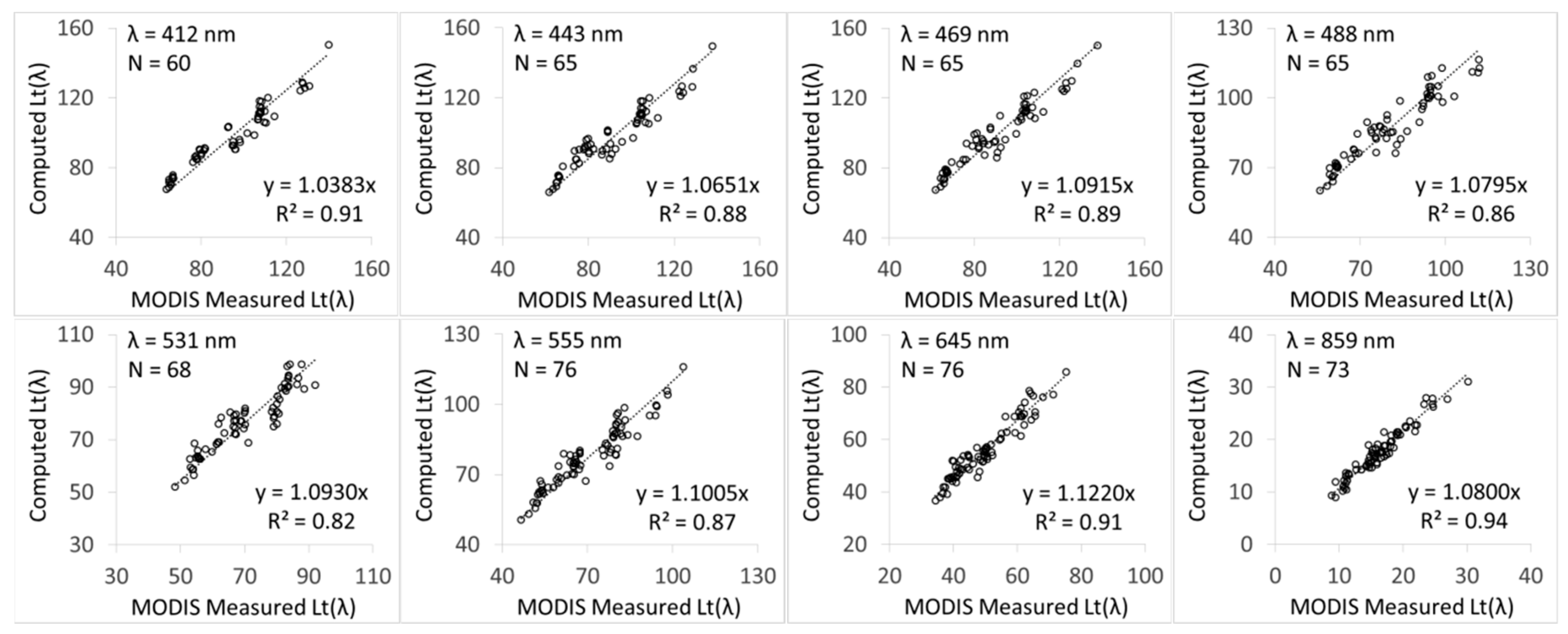
4.1. Vicarious Calibration Results

To perform the vicarious calibration of the MODIS-Aqua VIS-NIR bands, we used the coincident in situ R_rs(λ) measurements with the eight scenes of the MODIS-Aqua images, including A20060090445, A20062110520, A20070080510, A20071160535, A20090730540, A20091070530, A20122920525, and A20142990510. Using the atmospheric parameters computed with the SeaDAS 7.2 and the in situ-measured R_rs(λ), we calculated the L_t(λ) in the eight VIS-NIR bands. Figure 3 shows the scatter plots of the computed L_t(λ) and MODIS-measured L_t(λ). By performing a regression between the computed L_t(λ) and MODIS-measured L_t(λ), we obtained the vicarious calibration results.

Table 3. The regional vicarious calibration results for the MODIS-Aqua visible and near infrared (NIR) bands using the in situ R_rs(λ) in the highly turbid Lake Taihu with the (1240, 1640)-based atmospheric correction algorithm. The default gains in SeaDAS 7.2 are also shown in this table.

Band (nm)	412	443	469	488	531	555	645	859
gain (This study)	1.0383	1.0651	1.0915	1.0795	1.0930	1.1005	1.1220	1.0800
gain (SeaDAS 7.2 default)	0.9722	0.9872	1.0139	0.9923	0.9995	1.0014	1.0253	1.0184

lists the “gain” of the eight VIS-NIR land bands.

4.2. Atmospheric Correction Accuracy Assessment

We compared the atmospheric correction accuracy of the three methods, i.e., the (1640, 2130), (1240, 2130)-Ite, and (1240, 2130)-Cal. First, we computed their atmospheric correction accuracy with matchups for the in situ R_rs(λ) measurements coincident with the MODIS-Aqua image pixels. Then, we further compared the typical atmospheric correction result images using the three methods.

4.2.1. Comparison of Atmospheric Correction Accuracy

Figure 4 shows the scatter plots for the matchups of the in situ R_rs(λ) measurements coincident with the atmospheric correction results for the MODIS-Aqua using the three methods, i.e., the (1640, 2130), (1240, 2130)-Ite, and (1240, 2130)-Cal. The points for the (1240, 2130)-Cal results were divided into calibration points, referred to as (1240, 2130)-Cal (Cal), and validation points, referred to as (1240, 2130)-Cal (Val).

Table 4. The accuracy, based on the matchups, of the in situ R_rs(λ) measurements coincident with the atmospheric correction results for MODIS-Aqua using the three methods, i.e., the (1640, 2130), (1240, 2130)-Ite, and (1240, 2130)-Cal. For the (1240, 2130)-Cal, accuracies were computed for both the total and validation matchup data, which are reported as (1240, 2130)-Cal (Total) and (1240, 2130)-Cal (Val), respectively. The valid matchup numbers vary for the different bands and with respect to the atmospheric correction method because the valid atmospheric-corrected R_rs(λ) value must be positive and the coefficients of variation must be smaller than 40% in the 3×3 window that surrounds the coincident in situ R_rs(λ) measurements.

Approach	Band (nm)	Valid matchup numbers	Rrs range (sr−1)	ARE	RMSE (sr−1)	rRMSE	r
(1640, 2130)	469	50	0.004–0.035	52%	0.015	62%	0.15
	555	89	0.005–0.051	28%	0.013	35%	0.58
	645	92	0.002–0.054	24%	0.010	31%	0.75
	859	77	0.002–0.029	26%	0.004	41%	0.81
(1240, 2130)-Ite	469	95	0.003–0.025	29%	0.009	36%	0.25
	555	112	0.010–0.039	28%	0.014	33%	0.25
	645	112	0.007–0.035	26%	0.012	31%	0.67
	859	109	0002–0.030	40%	0.006	96%	0.69
(1240, 2130)-Cal (Total)	469	98	0.002–0.033	33%	0.009	40%	0.58
	555	129	0.014–0.048	15%	0.007	20%	0.70
	645	130	0.008–0.050	14%	0.006	19%	0.84
	859	122	0.002–0.028	22%	0.003	29%	0.90
(1240, 2130)-Cal (Val)	469	25	0.002–0.031	39%	0.010	47%	0.78
	555	51	0.014–0.048	20%	0.008	24%	0.77
	645	52	0.008–0.050	18%	0.007	24%	0.83
	859	46	0.002–0.028	28%	0.003	35%	0.88

lists the calculated ARE, RMSE, rRMSE, and r. The accuracy of the atmospheric correction results for the (1240, 2130)-Cal method was computed using both validation and total matchups.

Based on Figure 4, we observe that the R_rs(λ) results from the (1240, 2130)-Cal method are closer to the 1:1 line compared with the results from the (1640, 2130) and (1240, 2130)-Ite methods. For the R_rs(λ) results from the (1240, 2130)-Cal method, the distribution of the calibration points (referred to as (1240, 2130)-Cal(Cal)) are similar to those of the validation points (referred to as (1240, 2130)-Cal(Val)). For the R_rs(λ) results at different bands from the (1240, 2130)-Cal method, the R_rs(λ) values at the 555, 645, and 859 nm bands are closer to the 1:1 line while the R_rs(λ) results at the 469 nm band show a slight scatter.

We can further analyze the accuracy reported in Table 4. First, the valid matchup numbers from the (1640, 2130) method are the smallest, which is mainly due to the fact 70% of the detectors are inoperable in the 1640 nm band. Valid matchup numbers for the (1240, 2130)-Ite method are also smaller than those based on the (1240, 2130)-Cal method, which is mainly due to the fact that the (1240, 2130)-Ite method does not work on several images absent of clear water. Therefore, the (1240, 2130)-Cal method yielded the most valid matchup numbers, which indicates that it is a more robust method. Second, for the ARE, RMSE, and rRMSE, the valid matchup numbers from the (1240, 2130)-Cal method are the smallest. Third, for r, the valid matchup numbers from the (1240, 2130)-Cal method are the largest. Lastly, the difference between these accuracies for the (1240, 2130)-Cal (Total) and (1240, 2130)-Cal (Val) methods are similar. Therefore, these results suggest that the (1240, 2130)-Cal method has the highest accuracy and robustness.

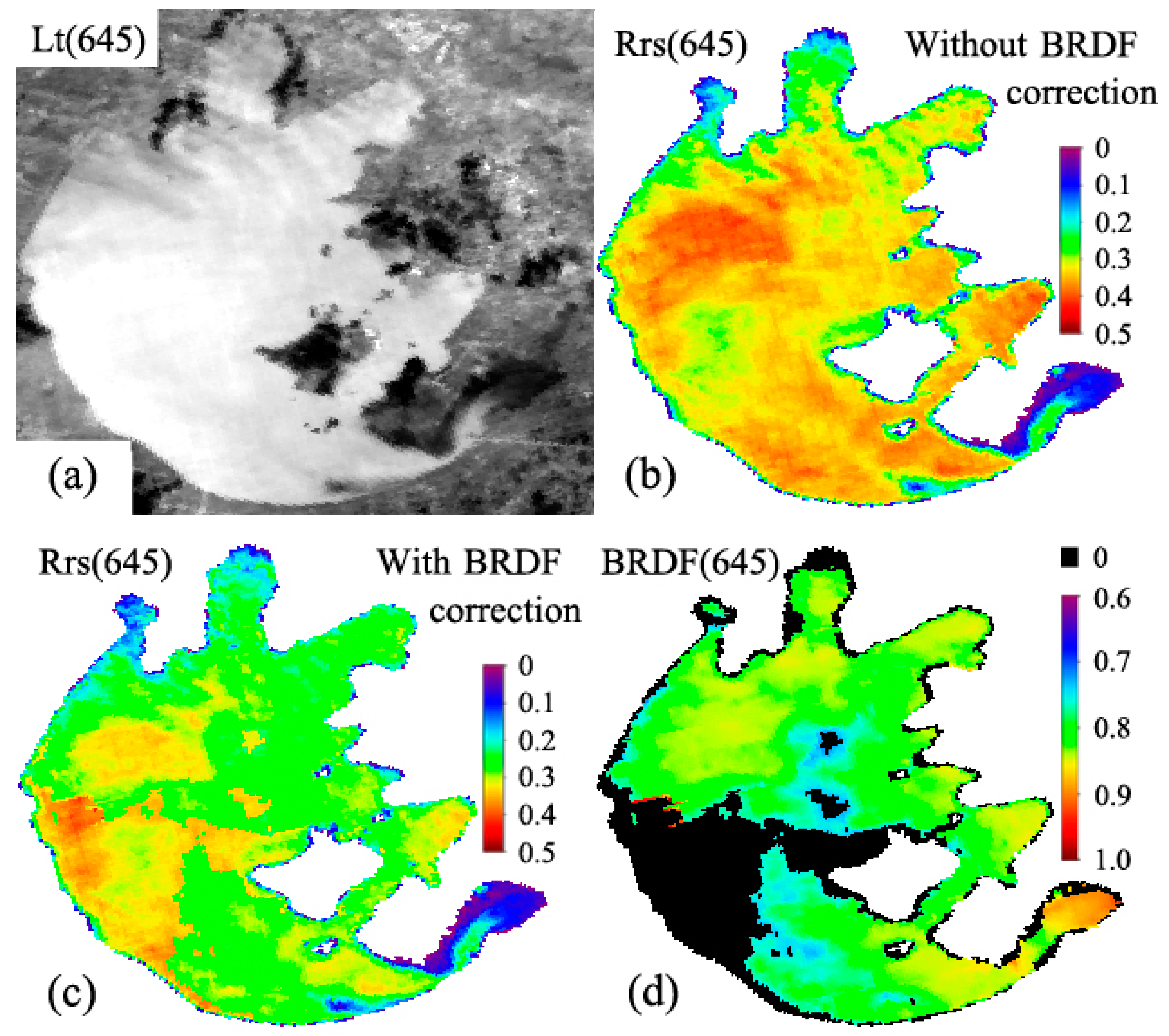
4.2.2. Comparison of Atmospheric-Corrected Images

We used a scene of a MODIS-Aqua image, acquired on April 26, 2009, named A20091160520, to compare the atmospheric-corrected R_rs images based on the (1640, 2130), (1240, 2130)-Ite, and (1240, 2130)-Cal methods. We set the spatial resolution of the atmospheric-corrected R_rs result image at 250 m. The R_rs(645) and R_rs(859) images had finer spatial patterns since their original spatial resolution was 250 m and did not require spatial interpolation. Figure 5 shows a comparison of the atmospheric-corrected R_rs(645) and R_rs(859) images based on the three different methods. There are five coincident in situ R_rs measurements and Figure 5a shows their locations as red dots. We further compared the five matchups of the in situ R_rs spectra with the corresponding atmospheric-corrected R_rs spectra in Figure 6.

Table 5. The average relative error (ARE) of the five matchups for the in situ R_rs spectra with the corresponding atmospheric-corrected R_rs spectra from the MODIS-Aqua image acquired on 26 April 2009, processed using the three different methods.

	Band(nm)	412	443	469	488	531	555	645	859	Mean
Approach
(1640, 2130)		25%	18%	15%	13%	10%	9%	7%	13%	14%
(1240, 2130)-Ite		24%	22%	23%	21%	13%	19%	16%	17%	19%
(1240, 2130)-Cal		17%	14%	11%	11%	9%	7%	6%	13%	11%

lists the average ARE of these five matchups.

Based on Figure 5, we observe that there are similar spatial patterns in the retrieved R_rs(645) and R_rs(859) images from the different atmospheric correction methods. There is significant noise and areas of atmospheric correction failure in the retrieved R_rs(645) and R_rs(859) images from the (1640, 2130) method, which is mainly due to the inoperable detectors in the 1640 nm band. Most areas of the retrieved R_rs(645) and R_rs(859) images based on the (1240, 2130)-Ite method were underestimated compared with those retrieved by the (1640, 2130) and (1240, 2130)-Cal methods, which is possibly due to the inappropriate interpolation of aerosol models from clear water. Based on Figure 6, we observe that the R_rs(λ) spectra retrieved by the (1240, 2130)-Cal method are, overall, the closest to the in situ-measured R_rs(λ) spectra, though the match-ups of (1) and (3) show a better correspondence with the R_rs(λ) spectra retrieved by the (1640, 2130) method. This is also observable based on the average ARE listed in Table 5, which is 11% for the (1240, 2130)-Cal method and 14% for the (1640, 2130) method. As for the retrieved R_rs(λ) spectral shapes, the (1640, 2130) method retrieves even better spectral shapes than the (1240, 2130)-Cal method. Considering all these factors, the results in Figure 5 and Figure 6 and Table 5 indicate that the (1240, 2130)-Cal method produces the best overall R_rs(λ) results.

5. Discussion

5.1. Effects of the BRDF Correction

The SeaDAS 7.2 default BRDF correction model is the Morel f/Q model, which is an iterative model based on chlorophyll-a [44,45]. This model performs well in clear open ocean waters but has problems when applied to highly turbid coastal and inland waters [27]. We used a scene from a MODIS-Aqua image, acquired on 9 January 2006, named A20060090445, to discuss the BRDF problem.

We used the (1240, 2130)-Cal approach to perform atmospheric correction of this image twice. We did not perform BRDF correction (brdf_opt = 0) the first time, and for the second, we set the BRDF correction as the default value. Figure 7b,c show the atmospheric-corrected R_rs(645) results with and without the default BRDF correction, respectively. We further show the BRDF correction factor in Figure 7d, which was computed during the atmospheric correction process with the default BRDF correction.

Based on Figure 7, we observe that the R_rs(645) image without BRDF correction is smooth along the entire lake and the spatial pattern is similar to that of L_t(645). The R_rs(645) image with BRDF correction, however, has several clear jumps mainly located at the center and southwestern areas of the lake. By comparing these images with the BRDF correction factor image, these jumps occur at the edges of the black areas. The value of these black areas is zero, which indicates that the BRDF correction model failed in these areas and did not perform BRDF correction. Therefore, Figure 7 confirms that the SeaDAS 7.2 default BRDF correction is not suitable for highly turbid waters. Unfortunately, there are no other existing operational BRDF correction models for highly turbid waters.

Fortunately, due to the multi-scattering of light in highly turbid waters, the BRDF of highly turbid water is weaker than that of clear ocean water [27]. We can, therefore, temporally ignore the BRDF correction for highly turbid waters, especially when the viewing zenith angle is not large, which will yield reasonable atmospheric-corrected results. For image pixels with large viewing zenith angles, which can be obtained from the Hisatzen field in l2flags, the atmospheric-corrected results should be used cautiously.

5.2. Uncertainty and Applicability Analysis

Except for the BRDF correction, there are several other sources of error in the SWIR-based atmospheric correction method, including the noise in the SWIR bands, the inaccurate aerosol model, and other parameter settings in the SeaDAS 7.2, as well as the non-negligible water-leaving radiance in the 1240 nm band in certain extremely turbid waters. By incorporating the vicarious calibration results into the atmospheric correction process, these errors cancel out to some extent, especially in the macroscopic view. This suggests that the atmospheric-corrected results of a specific image may contain certain errors but that the vicarious calibration significantly cancels out the overall error.

The atmospheric corrections had better accuracy at the 555 (green light), 645 (red light), and 859 nm (NIR) wavelengths than those at the 469 nm (blue light) wavelength, which is possibly due to two reasons. On one hand, blue light is farther from the SWIR bands than the green, red, and NIR bands, such that the aerosol scattering errors are possibly due to derivation over a longer spectral distance because the errors associated with the SWIR bands, aerosol models, and other sources of error may increase during derivation over a long distance. On the other hand, in situ R_rs measurements are based on the above-water method and the determination of the skylight reflectance at the air–water interface, r_sky, which also has associated uncertainty. Since skylight has increased at the blue light wavelength, the error associated with determining r_sky causes higher uncertainty in the computed R_rs results for blue light. Therefore, the atmospheric-corrected R_rs results at 469 nm (blue light) should be used cautiously. While blue light is highly absorbed by high concentrations of suspended particulate matter and color dissolved organic matter (CDOM) in highly turbid waters, the R_rs for blue light is seldom used to retrieve chlorophyll-a and suspended particulate matter in highly turbid waters [28,29,46,47,48].

The vicarious calibration results are mainly applicable to Lake Taihu as these are based on the coincident in situ-measured R_rs data from the lake; however, these may also be applicable to other highly turbid waters with similar optical and aerosol optical properties above water. Even if the calibration results may not be applicable to some waters, the procedure used in this study can be applied to these waters in general, by using the coincident in situ-measured R_rs data from these waters to obtain new vicarious calibration coefficients. We expect to validate and extend the present approach to other highly turbid waters in the near future.

6. Conclusions

In this study, we performed regional vicarious calibration of the MODIS-Aqua SWIR (1240, 2130)-based atmospheric correction approach using the in situ water surface reflectance data measured in the highly turbid Lake Taihu during different seasons. We then verified the accuracy of the (1240, 2130)-based atmospheric correction approach with the vicarious calibrated results and compared the results with the other approaches. The main findings of this study are as follows.

First, the vicarious calibration was performed based on the in situ R_rs measurements from Lake Taihu coincident with eight scenes of the MODIS-Aqua images. The obtained vicarious calibration coefficient gains for the eight MODIS-Aqua visible and NIR bands at 412, 443, 469, 488, 531, 555, 645, and 859 nm were 1.0383, 1.0651, 1.0915, 1.0795, 1.0930, 1.1005, 1.1220, and 1.0800, respectively.

Second, through the regional vicarious calibration of the VIS-NIR bands, the (1240, 2130)-based atmospheric correction approach yielded good results for the R_rs retrievals at the 555, 645, and 859 nm bands for Taihu Lake, with AREs of 15%, 14%, 22% for the 555, 645, and 859 nm bands, respectively, with no significant bias.

Further comparison with the (1240, 2130)-based iterative approach (i.e., the (1240, 2130)-Ite) and the (1640, 2130)-based approach showed that the vicarious calibrated (1240, 2130)-based approach had the best accuracy and robustness.

Finally, our results suggest that the SeaDAS 7.2 default BRDF correction model is not suitable for highly turbid waters since it is weaker than that of clear ocean waters. Therefore, we do not recommend the use of the BRDF correction for the atmospheric correction of highly turbid waters.

These results show that the regional vicarious calibration of the (1240, 2130)-based atmospheric correction approach is applicable to the highly turbid Lake Taihu. This approach may also be applicable to other highly turbid inland waters with similar optical and aerosol optical properties above water but requires further validation.

References

1. Gordon, H.R.; Wang, M. Retrieval of water-leaving radiance and aerosol optical thickness over the oceans with SeaWiFS: A preliminary algorithm. Appl. Optics. 1994, 33, 443–452. [Google Scholar] [CrossRef] [PubMed]
2. McClain, C.R. A decade of satellite ocean color observations. Annu. Rev. Mar. Sci. 2009, 1, 19–42. [Google Scholar] [CrossRef] [PubMed]
3. Ruddick, K.G.; Ovidio, F.; Rijkeboer, M. Atmospheric correction of SeaWiFS imagery for turbid coastal and inland waters. Appl. Optics. 2000, 39, 897–912. [Google Scholar] [CrossRef] [PubMed] [Green Version]
4. Siegel, D.A.; Wang, M.; Maritorena, S.; Robinson, W. Atmospheric correction of satellite ocean color imagery: the black pixel assumption. Appl. Opt. 2000, 39, 3582–3591. [Google Scholar] [CrossRef] [PubMed]
5. Stumpf, R.; Arnone, R.; Gould, R.W.; Martinolich, P.M.; Ransibrahmanakul, V. A partially coupled ocean-atmosphere model for retrieval of water-leaving radiance from SeaWiFS in coastal waters. NASA Tech. Memo. 2003, 206892, 51–59. [Google Scholar]
6. Lavender, S.J.; Pinkerton, M.H.; Moore, G.F.; Aiken, J.; Blondeau-Patissier, D. Modification to the atmospheric correction of SeaWiFS ocean colour images over turbid waters. Cont. Shelf. Res. 2005, 25, 539–555. [Google Scholar] [CrossRef]
7. Bailey, S.W.; Franz, B.A.; Werdell, P.J. Estimation of near-infrared water-leaving reflectance for satellite ocean color data processing. Opt. Express 2010, 18, 7521–7527. [Google Scholar] [CrossRef] [PubMed]
8. Hu, C.; Carder, K.L.; Muller-Karger, F.E. Atmospheric Correction of SeaWiFS Imagery over Turbid Coastal Waters: A Practical Method. Remote Sens. Environ. 2000, 74, 195–206. [Google Scholar] [CrossRef]
9. Wang, M.; Wei, S. Estimation of ocean contribution at the MODIS near-infrared wavelengths along the east coast of the US: Two case studies. Geophys. Res. Lett. 2005, 32, 370. [Google Scholar] [CrossRef]
10. Wang, M.; Shi, W. The NIR-SWIR combined atmospheric correction approach for MODIS ocean color data processing. Opt. Express 2007, 15, 15722–15733. [Google Scholar] [CrossRef] [Green Version]
11. Wang, M.; Liu, X. The MODIS-SWIR Algorithm Theoretical Basis Document Version 1.0. In NOAA NESDIS STAR; 2012; 40p. Available online: https://www.star.nesdis.noaa.gov/sod/mecb/color/documents/SWIR_ATBD_ver1-2012.pdf (accessed on 1 July 2019).
12. Hale, G.M.; Querry, M.R. Optical Constants of Water in the 200-nm to 200-μm Wavelength Region. Appl. Optics. 1973, 12, 555–563. [Google Scholar] [CrossRef] [PubMed]
13. Wang, M.; Tang, J.; Shi, W. MODIS-derived ocean color products along the China east coastal region. Geophys. Res. Lett. 2007, 34, L06611. [Google Scholar] [CrossRef]
14. Wang, M.; Son, S.; Shi, W. Evaluation of MODIS SWIR and NIR-SWIR atmospheric correction algorithms using SeaBASS data. Remote Sens. Environ. 2009, 113, 635–644. [Google Scholar] [CrossRef]
15. Wang, M.; Shi, W.; Tang, J. Water property monitoring and assessment for China’s inland Lake Taihu from MODIS-Aqua measurements. Remote Sens. Environ. 2011, 115, 841–854. [Google Scholar] [CrossRef]
16. Zhang, M.; Ma, R.; Li, J.; Zhang, B.; Duan, H. A Validation Study of an Improved SWIR Iterative Atmospheric Correction Algorithm for MODIS-Aqua Measurements in Lake Taihu, China. IEEE. Trans. Geosci. Remote Sens. 2014, 52, 4686–4695. [Google Scholar] [CrossRef]
17. Wang, M.; Son, S.; Zhang, Y.; Shi, W. Remote Sensing of Water Optical Property for China’s Inland Lake Taihu Using the SWIR Atmospheric Correction With 1640 and 2130 nm Bands. IEEE J. Sel. Topics Appl. Earth Observ. Remote Sens. 2013, 6, 2505–2516. [Google Scholar] [CrossRef]
18. Gordon, H.R. In-orbit calibration strategy for ocean color sensors. Remote Sens. Environ. 1998, 63, 265–278. [Google Scholar] [CrossRef]
19. Wang, M. In-orbit vicarious calibration for ocean color and aerosol products. In Proceedings of the 2005 IEEE International Geoscience and Remote Sensing Symposium, 2005, IGARSS ’05, Seoul, South Korea, 29 July 2005; 2005. [Google Scholar] [CrossRef]
20. Franz, B.A.; Bailey, S.W.; P Jeremy, W.; Mcclain, C.R. Sensor-independent approach to the vicarious calibration of satellite ocean color radiometry. Appl. Optics. 2007, 46, 5068–5082. [Google Scholar] [CrossRef]
21. Dash, P.; Walker, N.; Mishra, D.; D’Sa, E.; Ladner, S. Atmospheric Correction and Vicarious Calibration of Oceansat-1 Ocean Color Monitor (OCM) Data in Coastal Case 2 Waters. Remote Sens. 2007, 4, 1716–1740. [Google Scholar] [CrossRef]
22. Zibordi, G.; Mélin, F.; Voss, K.J.; Johnson, B.C.; Franz, B.A.; Kwiatkowska, E.; Huot, J.-P.; Wang, M.; Antoine, D. System vicarious calibration for ocean color climate change applications: Requirements for in situ data. Remote Sens. Environ. 2015, 159, 361–369. [Google Scholar] [CrossRef]
23. Wang, M.; Shi, W.; Jiang, L.; Voss, K. NIR- and SWIR-based on-orbit vicarious calibrations for satellite ocean color sensors. Opt. Express 2016, 24, 20437–20453. [Google Scholar] [CrossRef] [PubMed]
24. Li, J.; Hu, C.; Shen, Q.; Barnes, B.B.; Murch, B.; Feng, L.; Zhang, M.; Zhang, B. Recovering low quality MODIS-Terra data over highly turbid waters through noise reduction and regional vicarious calibration adjustment: A case study in Taihu Lake. Remote Sens. Environ. 2017, 197, 72–84. [Google Scholar] [CrossRef]
25. Concha, J.; Mannino, A.; Franz, B.; Bailey, S.; Kim, W. Vicarious calibration of GOCI for the SeaDAS ocean color retrieval. Int. J. Remote Sens. 2019, 40, 3984–4001. [Google Scholar] [CrossRef]
26. Clark, D.K.; Gordon, H.R.; Voss, K.J.; Ge, Y.; Broenkow, W.; Trees, C. Validation of atmospheric correction over the ocean. J. Geophys. Res. - Atmos. 1997, 102, 17209–17217. [Google Scholar] [CrossRef]
27. Li, J.; Shen, Q.; Zhang, B.; Chen, D. Retrieving total suspended matter in Lake Taihu from HJ-CCD near-infrared band data. Aquat. Ecosyst. Health. 2014, 17, 280–289. [Google Scholar] [CrossRef]
28. Shi, K.; Zhang, Y.; Zhu, G.; Liu, X.; Zhou, Y.; Xu, H.; Qin, B.; Liu, G.; Li, Y. Long-term remote monitoring of total suspended matter concentration in Lake Taihu using 250m MODIS-Aqua data. Remote Sens. Environ. 2015, 164, 43–56. [Google Scholar] [CrossRef]
29. Zhang, B.; Li, J.; Shen, Q.; Chen, D. A bio-optical model based method of estimating total suspended matter of Lake Taihu from near-infrared remote sensing reflectance. Environ. Monit. Assess. 2008, 145, 339–347. [Google Scholar] [CrossRef]
30. Duan, H.; Ma, R.; Hu, C. Evaluation of remote sensing algorithms for cyanobacterial pigment retrievals during spring bloom formation in several lakes of East China. Remote Sens. Environ. 2012, 126, 126–135. [Google Scholar] [CrossRef]
31. Duan, H.; Ma, R.; Loiselle, S.A.; Shen, Q.; Yin, H.; Zhang, Y. Optical characterization of black water blooms in eutrophic waters. Sci. Total Environ. 2014, 482, 174–183. [Google Scholar] [CrossRef]
32. Sun, D.Y.; Yun, M.L.; Qiao, W.; Lv, H.; Cheng, F.L.; Chang, C.H.; Shao, Q.G. Detection of Suspended-Matter Concentrations in the Shallow Subtropical Lake Taihu, China, Using the SVR Model Based on DSFs. IEEE Geosci. Remote Sens. 2010, 7, 816–820. [Google Scholar] [CrossRef]
33. Hu, C.; Lee, Z.; Ma, R.; Yu, K.; Li, D. MODIS observations of cyanobacteria blooms in Taihu Lake, China. J. Geophys. Res. 2010, 115, 1–20. [Google Scholar] [CrossRef]
34. Le, C.; Li, Y.; Zha, Y.; Sun, D.; Huang, C.; Zhang, H. Remote estimation of chlorophyll a in optically complex waters based on optical classification. Remote Sens. Environ. 2011, 115, 725–737. [Google Scholar] [CrossRef]
35. Lyu, H.; Wang, Y.; Jin, Q.; Shi, L.; Li, Y.; Wang, Q. Developing a semi-analytical algorithm to estimate particulate organic carbon (POC) levels in inland eutrophic turbid water based on MERIS images: A case study of Lake Taihu. Int. J. Appl. Earth Obs. Geoinf. 2017, 62, 69–77. [Google Scholar] [CrossRef]
36. Ma, R.; Duan, H.; Lü, C.; Loiselle, S. Unusual links between inherent and apparent optical properties in shallow lakes, the case of Taihu Lake. Hydrobiologia 2011, 7, 49–158. [Google Scholar] [CrossRef]
37. Qi, L.; Hu, C.; Duan, H.; Cannizzaro, J.; Ma, R. A novel MERIS algorithm to derive cyanobacterial phycocyanin pigment concentrations in a eutrophic lake: Theoretical basis and practical considerations. Remote Sens. Environ. 2014, 154, 298–317. [Google Scholar] [CrossRef]
38. Mueller, J.L.; Morel, A.; Frouin, R.; Davis, C.; Arnone, R.; Carder, K.; Lee, Z.P.; Steward, R.G.; Hooker, S.; Holben, B.; et al. Ocean optics protocols for satellite ocean color sensor validation, Revision 4, Volume III: radiometric measurements and data analysis protocols. Natl. Aeronaut. Space Adm. Rep. 2003, 21621, 1–72. [Google Scholar]
39. Mobley, C.D. Estimation of the remote-sensing reflectance from above-surface measurements. Appl. Optics. 1999, 38, 7442–7455. [Google Scholar] [CrossRef]
40. Sun, D.; Li, Y.; Le, C.; Shi, K.; Huang, C.; Gong, S.; Yin, B. A semi-analytical approach for detecting suspended particulate composition in complex turbid inland waters (China). Remote Sens. Environ. 2013, 134, 92–99. [Google Scholar] [CrossRef]
41. Zhang, F.; Li, J.; Qian, S.; Bing, Z.; Wu, C.; Wu, Y.; Wang, G.; Wang, S.; Lu, Z. Algorithms and Schemes for Chlorophyll a Estimation by Remote Sensing and Optical Classification for Turbid Lake Taihu, China. IEEE J. Sel. Topics Appl. Earth Observ. Remote Sens. 2017, 8, 350–364. [Google Scholar] [CrossRef]
42. Shen, Q.; Li, J.; Zhang, F.; Sun, X.; Li, J.; Li, W.; Zhang, B. Classification of Several Optically Complex Waters in China Using in Situ Remote Sensing Reflectance. Remote Sens. 2015, 7, 14731–14756. [Google Scholar] [CrossRef] [Green Version]
43. Gordon, H.R.; Voss, K.J. MODIS Normalized Water-Leaving Radiance, ‭Algorithm Theoretical ‭‬Basis Document (MODIS 18); Version 5; University Miami: Coral Gables, FL, USA, 2004. [Google Scholar]
44. Morel, A.; Gentili, B. Diffuse reflectance of oceanic waters. III. Implication of bidirectionality for the remote-sensing problem. Appl. Optics. 1996, 35, 4850–4862. [Google Scholar] [CrossRef] [PubMed]
45. Morel, A.; Antoine, D.; Gentili, B. Bidirectional reflectance of oceanic waters: accounting for Raman emission and varying particle scattering phase function. Appl. Optics. 2002, 41, 6289–6306. [Google Scholar] [CrossRef] [PubMed]
46. Wang, H.; Hladik, C.M.; Huang, W.; Milla, K.; Edmiston, L.; Harwell, M.; Schalles, J. Detecting the spatial and temporal variability of chlorophyll-a concentration and total suspended solids in Apalachicola Bay, Florida using MODIS imagery. Int. J. Remote Sens. 2010, 31, 439–453. [Google Scholar] [CrossRef]
47. Le, C.; Hu, C.; English, D.; Cannizzaro, J.; Chen, Z.; Feng, L.; Boler, R.; Kovach, C. Towards a long-term chlorophyll-a data record in a turbid estuary using MODIS observations. Prog. Oceanogr. 2013, 109, 90–103. [Google Scholar] [CrossRef]
48. Nechad, B.; Ruddick, K.G.; Park, Y. Calibration and validation of a generic multisensor algorithm for mapping of total suspended matter in turbid waters. Remote Sens. Environ. 2010, 114, 854–866. [Google Scholar] [CrossRef]
Figure 1. Maps of the location of Lake Taihu, China, and the 377 in situ water sampling stations used during the 12 cruise surveys performed between 2005 and 2014.
Remotesensing 11 01670 g001
Figure 2. The Rrs spectra measured in Lake Taihu from the 12 cruise surveys performed in (a) October 2005, (b) January 2006, (c) July to August 2006, (d) October 2006, (e) January 2007, (f) April 2007, (g) March 2009, (h) April 2009, (i) October 2012, (j) May 2013, (k) July 2014, and (l) October 2014.
Remotesensing 11 01670 g002
Figure 3. A comparison between the moderate resolution imaging spectroradiometer (MODIS)-Aqua measured Lt(λ) in Lake Taihu with the computed Lt(λ) via the in situ-measured Rrs(λ) and atmospheric correction parameters calculated with the SeaDAS 7.2. The units for the MODIS-measured and computed Lt(λ) are W m−2 μm−1 sr−1.
Remotesensing 11 01670 g003
Figure 4. The scatter plots of the matchups for the in situ Rrs(λ) measurements coincident with the atmospheric correction results of MODIS-Aqua based on the three methods, i.e., the (1640, 2130), (1240, 2130)-Ite, and (1240, 2130)-Cal. The points for the (1240, 2130)-Cal results were divided into calibration, referred to as (1240, 2130)-Cal (Cal), and validation points, referred to as (1240, 2130)-Cal (Val). Table 4 lists the valid matchup numbers for each band based on each method.
Remotesensing 11 01670 g004
Figure 5. The atmospheric-corrected Rrs images of a scene from a MODIS-Aqua image acquired on 26 April 2009, based on the (1640, 2130), (1240, 2130)-Ite, and (1240, 2130)-Cal methods. (a) is the Lt(645) image, which shows the locations of the five coincident in situ Rrs measurements as red dots. (bd) are the atmospheric-corrected Rrs(645) images based on the (1640, 2130), (1240, 2130)-Ite, and (1240, 2130)-Cal methods, respectively. (e) is the Lt(859) image. (fh) are the atmospheric-corrected Rrs(859) images based on the (1640, 2130), (1240, 2130)-Ite, and (1240, 2130)-Cal methods, respectively. The (1240, 2130)-Cal method retrieved an AOT(555) = 0.33 (Mean) ± 0.10 (Std).
Remotesensing 11 01670 g005
Figure 6. A comparison of the five matchups for the in situ Rrs spectra with corresponding atmospheric-corrected Rrs spectra from the MODIS-Aqua image acquired on 26 April 2009, which was processed using the three different methods. The five subfigures show the comparison results on the five in situ locations, the red dots in Figure 5a.
Remotesensing 11 01670 g006
Figure 7. The atmospheric-corrected Rrs(645) images of a scene of a MODIS-Aqua image acquired on 9 January 2006, using the (1240, 2130)-Cal method. (a) is the Lt(645) image. (b,c) are the atmospheric-corrected results without BRDF correction and with the default BRDF correction, respectively. (d) is the BRDF correction factor computed during the atmospheric correction process with the default BRDF correction.
Remotesensing 11 01670 g007