Removal of Chlorophyll-a Spectral Interference for Improved Phycocyanin Estimation from Remote Sensing Reflectance


Department of Earth Sciences, Indiana University—Purdue University at Indianapolis, Indianapolis, IN 46202, USA
*
Author to whom correspondence should be addressed.
Remote Sens. 2019, 11(15), 1764; https://doi.org/10.3390/rs11151764
Submission received: 9 June 2019
/
Revised: 20 July 2019
/
Accepted: 24 July 2019
/
Published: 26 July 2019
(This article belongs to the Special Issue Satellite Monitoring of Water Quality and Water Environment)
Abstract
:Monitoring cyanobacteria is an essential step for the development of environmental and public health policies. While traditional monitoring methods rely on collection and analysis of water samples, remote sensing techniques have been used to capture their spatial and temporal dynamics. Remote detection of cyanobacteria is commonly based on the absorption of phycocyanin (PC), a unique pigment of freshwater cyanobacteria, at 620 nm. However, other photosynthetic pigments can contribute to absorption at 620 nm, interfering with the remote estimation of PC. To surpass this issue, we present a remote sensing algorithm in which the contribution of chlorophyll-a (chl-a) absorption at 620 nm is removed. To do this, we determine the PC contribution to the absorption at 665 nm and chl-a contribution to the absorption at 620 nm based on empirical relationships established using chl-a and PC standards. The proposed algorithm was compared with semi-empirical and semi-analytical remote sensing algorithms for proximal and simulated satellite sensor datasets from three central Indiana reservoirs (total of 544 sampling points). The proposed algorithm outperformed semi-empirical algorithms with root mean square error (RMSE) lower than 25 µg/L for the three analyzed reservoirs and showed similar performance to a semi-analytical algorithm. However, the proposed remote sensing algorithm has a simple mathematical structure, it can be applied at ease and make it possible to improve spectral estimation of phycocyanin from space. Additionally, the proposed showed little influence from the package effect of cyanobacteria cells.
1. Introduction
Cyanobacteria, also known as blue-green algae, has been observed in lentic freshwater systems worldwide [1]. Their success in aquatic systems has been associated with ecophysiological strategies which allow them to exploit the variability in different environmental factors, specifically nutrient over-enrichment and hydrologic alterations to ecosystems [2,3,4]. However, the presence of cyanobacteria, especially in water supply aquatic systems, is a worldwide concern due to the ability of some species to produce toxic secondary metabolites. Theses metabolites cause health effects in mammals (including humans) affecting several systems such as: the hepatopancreatic, digestive, endocrine, dermal, and nervous systems [5,6].
The traditional management of cyanobacteria focus on the in situ collection of water samples for monitoring their cell abundance, biomass and indicators such as chlorophyll-a (chl-a) and microcystin. However, these methods are expensive, time consuming [7], and have difficulty capturing the spatial and temporal heterogeneity [8]. An alternative to traditional monitoring is the use of remote sensing [9,10,11,12,13,14,15]. Initially, cyanobacterial biomass was remotely estimated from chl-a concentration because chl-a is the primary and dominant photosynthetic pigment and thus an appropriate proxy for cyanobacterial biomass [16]. However, chl-a is not an accurate estimator of cyanobacterial biomass when cyanobacteria are not the dominant population. In a mixed phytoplankton population, chl-a is present in almost all phytoplankton groups [17]. Because of this, chl-a is not a reliable indicator of cyanobacteria. Therefore, remote sensing studies have evaluated the use of phycocyanin (PC) to estimate cyanobacterial concentration [9,10,11,12,13,14,18,19,20] in aquatic systems.
Remote estimation of PC concentration is mainly based on its absorption and fluorescence features at 620–630 nm [9,10,21] and 650 nm [22,23], respectively. These spectral features have been used for developing empirical, semi-empirical, semi-analytical and quasi-analytical algorithms (QAA) [24]. Empirical and semi-empirical algorithms describe relationships between PC concentrations and radiometric data, whereas a semi-analytical algorithm or QAA use radiometric measurements to derive inherent optical properties (IOPs) which will be then used to estimate PC concentrations. Because of this difference, empirical and semi-empirical algorithms usually have a simple structure compared to a semi-analytical algorithm or QAA.
To reduce the interference of chl-a with the PC absorption retrieval at 620 nm, Simis et al. [9] used an empirical factor (ε) to relate the in vivo absorption of chl-a at 665 nm to its absorption at 620 nm (Equation (1)). The authors assumed that the absorption coefficient of phytoplankton (aphy) at 665 nm only depends on chl-a, and could be used as a proxy for achl-a. The PC absorption coefficient (aPC) at 620 nm was then calculated by subtracting achl-a from aphy at the same wavelength (Equation (2)).
Another algorithm aiming at mitigating chl-a interference with PC estimation was proposed by Mishra et al. [25]. In this algorithm, aPC at 620 nm was derived using two factors (ψ1 and ψ2), which are defined as the ratio of achl-a at 665 to that at 620 nm and the ratio of of aPC at 665 to that at 620 nm, respectively Equation (3).
Ruiz-Verdu et al. [26] compared the performance of empirical, semi-empirical, and semi-analytical algorithms in Spanish and Dutch lakes and concluded that the semi-empirical algorithm by Simis et al. [9] performed best for most of the study sites; for the remaining sites for which the algorithm proposed by Simis et al. [9] was not effective, Ruiz-Verdu et al. [26] pointed out that the algorithm proposed by Schalles and Yacobi [22] showed good performance. Ogashawara et al. [20] assessed semi-empirical algorithms for a tropical reservoir and catfish ponds and concluded that the algorithms proposed by Simis et al. [9] and Mishra et al. [19] had the best performances for the estimation of PC, and was less sensitive to the interference of chl-a. However, the algorithm proposed by Mishra et al. [19] cannot be adopted for the application of orbital satellites because uncommon spectral bands were proposed to use. Nonetheless, both studies [20,26] emphasized a significant interference of the chl-a absorption (achl-a) with the absorption coefficient at 620 nm, a critically important spectral diagnostic feature for the retrieval of PC concentration [27].
In fact, Simis et al.’s algorithm [9] was also based on the assumptions that the total backscattering coefficient (bb) does not vary with wavelength and the absorption by CDOM and detritus is negligible. However, these assumptions are invalid for inland and coastal waters. Therefore, Mishra et al. [25] proposed a QAA to compensate for the spectral interference of chl-a, CDOM and detritus at 620 nm. The algorithm proposed by Mishra et al. [25] has two main limitations. One is its dependence on an accurate aphy which can only be estimated via semi-analytical or quasi-analytical algorithms when the algorithm is applied to remote sensing measurements. However, these algorithms could commit an error as high as 26.04% when applied to estimate aphy [28], which can be introduced to the estimation of aPC [29]. The other limitation is its dependence on ψ1 and ψ2. The authors used an Rrs band ratio to approximate each factor (ψ1 and ψ2) and obtained a coefficient of determination (R2) of 0.89 for ψ1 but only 0.52 for ψ2. Thus, the weak correlation indicates that it is necessary to develop a reliable method for the estimation of aPC at 620 nm from space.
The main goal of this study is to propose a semi-empirical algorithm for improving PC estimation. In this new algorithm, PC’s contribution to the absorption of phytoplankton at 665 nm is taken into account in addition to the contribution of chl-a to the absorption phytoplankton at 620 nm. This differs from the algorithms shown in Equations (2) and (3) where the absorption coefficient of phytoplankton (aphy) at 665 nm was assumed to only depend on chl-a, and was used as a proxy for achl-a. The proposed algorithm was applied to proximal and evaluated by comparing with the performance of other semi-empirical and semi-analytical algorithms.
2. Materials and Methods
2.1. Algorithm Development
The derivation of an algorithm for remote sensing of inland waters starts with the relationship below Equation (4) [30,31]:
where a(λ) is the total absorption coefficient, bb is the backscattering coefficient, and f is the anisotropic factor of the downwelling light field [32].
a(λ) is usually expressed as the sum of the absorption coefficients of optically active constituents and the spectral absorption coefficient of pure water (aw(λ)) as indicated by Equation (5).
where aCDM(λ) is the spectral absorption coefficient of CDM (the sum of the spectral absorption coefficient of CDOM and detritus).
If aphy can be decomposed into achl-a and aPC, aphy at 620 nm and 665 nm can then be written as:
For chl-a and PC pigment standards, the following relationships are valid for achl-a at 620 nm and aPC at 665 nm:
If the values of A and B are close to 0, Equations (8) and (9) can be rearranged and plugged into Equations (6) and (7), resulting in:
Rearranging Equation (10) results in apc(620) to be:
Plugging Equation (11) into Equation (12) leads to an expression of apc(620):
Where φ1 and φ2 have constant values and can be calculated from Equations (8) and (9).
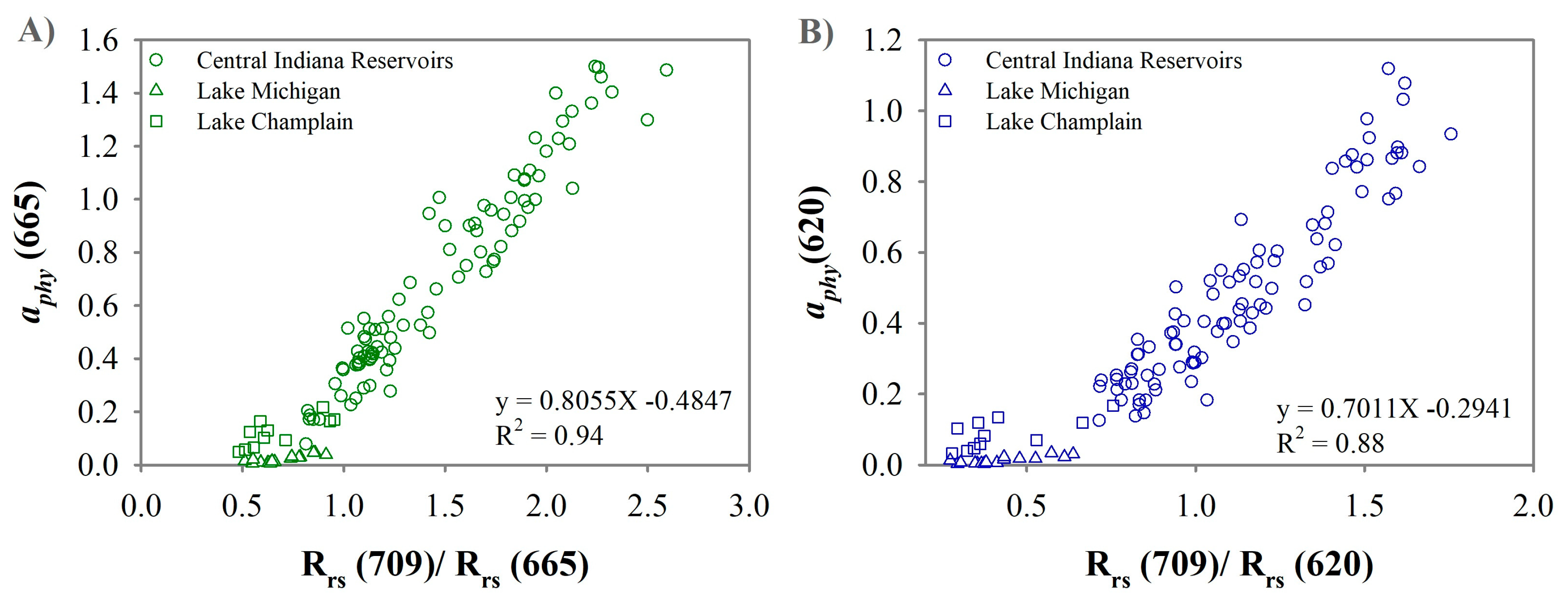
Obviously, aphy is needed to compute aPC at 620 nm, but it cannot be accurately measured via remote sensing measurements [28,29]. Although it is possible to estimate aphy from remote sensing measurements, recent reviews on this topic have shown that a simple band ratio is more feasible than a sophisticated method [20,33,34,35]. For example, the ratio of Rrs at 709 to 665 nm was demonstrated to be more efficient for chl-a estimation [33,34,35]. This ratio was proposed based on the absorption of chl-a at 665 nm and phytoplankton scattering around 709 nm. For PC estimation, the ratio of Rrs at 709 to 620 nm was more appropriate [20,26]. To confirm the feasibility of these band ratios for estimation of aphy at 620 nm and 665 nm, the Rrs datasets collected in central Indiana reservoirs (130 samples), Lake Champlain (11 samples) and Lake Michigan (16 samples) were used and the corresponding results are shown in Figure 1. The datasets from Lake Champlain and Lake Michigan were downloaded from SeaWiFS Bio-Optical Archive and Storage System (SeaBASS) archives [36]. SeaBASS archives contain high quality bio-optical global datasets which are suitable for tuning and validating ocean color algorithms [37]. The use of the SeaBASS datasets was to demonstrate the generalizability of the relationships based on the central Indiana aquatic systems for those that are not located in central Indiana.
The strong relationships presented on Figure 1 justify the use of Rrs (709)/Rrs (620) and Rrs (709)/Rrs (665) to replace the aphy at 620 and 665 nm, respectively. In this case, the absorption at 620 and 665 nm is only attributed to phytoplankton pigments (chl-a and PC) rather than CDOM, sediments and other phytoplankton pigments [9], and aPC at 620 nm can then be estimated by a semi-empirical algorithm Equation (14):
The proposed algorithm (hereafter called OGA19) can be used to estimate aPC at 620 nm from the Rrs at three different wavelengths (620, 665 and 709 nm) if φ1 and φ2 are known. It is worth noting that the three selected wavelengths are included in the spectral configuration of the Ocean and Land Colour Instrument (OLCI) onboard the European Satellite Sentinel-3.
2.2. Derivation of Parameters φ1 and φ2
To calculate the values of φ1 and φ2, standards for chl-a (C5753, chlorophyll-a from spinach) and PC (52468, C-Phycocyanin) were purchased from Sigma Aldrich and were first mixed with acetone and phosphate buffer solution (50 mM) respectively to form concentrated solutions of each pigment. Diluted solutions of chl-a and PC were then prepared using acetone and phosphate buffer respectively. Spectrophotometric analysis (Shimadzu UV-2401PC) was performed on the synthesized sample solutions to compute achl-a and aPC for each concentration. The values of achl-a and aPC at 620 and 665 nm were plotted in a scatter plot, and φ1 and φ2 were the slopes of the two linear regressions Equations (8) and (9). Once φ1 and φ2 are calculated, aPC (620) can be estimated with equation 14. In these linear relationships, pigment standards (in vitro) do not show the package effect which results in a reduced absorption for in vivo samples [38]. Simis et al. [9] used two constants to correct the package effect for the aphy at 620 and 665 nm (0.84 and 0.68 respectively).
2.3. Application and Evaluation of the Proposed Algorithm
2.3.1. Study Sites
Remote sensing and limnological datasets (Rrs, PC and chl-a concentrations) were created for Eagle Creek Reservoir (ECR, 39.8°N, 86.3°W), Geist Reservoir (GR, 39.9°N, 85.9°W), and Morse Reservoir (MR, 40.1°N, 86°W), central Indiana, USA. These urban aquatic systems supply water for the Indianapolis metropolitan area and have similar morphological characteristics such as depth (3.2–4.7 m), surface area (5–7.5 km2), volume (21–28 million m3), and residence time (55–70 days) [14]. This research uses data acquired from 2005 to 2007 and 2010 in the three study sites.
Proximal Remote Sensing Data
For proximal remote sensing data, an Ocean Optics USA 400 radiometer with fiber optics radiometer (Ocean Optics, Inc., Dunedin, FL, USA) was used to measure the above water downwelling irradiance (Ed(0+)) and below surface upwelling radiance (Lu(0−)). Rrs spectra were calculated following the procedure described in Gitelson et al. [39]. These data were linearly interpolated for 1 nm, and the specific wavelengths were retained to implement OGA19 as well as semi-empirical and semi-analytical algorithms for comparison. The number of in situ measurements was 219, 167 and 179 for ECR, GR and MR respectively.
Limnological Variable
Water samples and proximal remote sensing radiometric data were collected just below the water surface in each sampling station. Water samples were stored on ice in coolers until the samples were shipped back to the laboratory where water samples were filtered and frozen immediately to prevent pigment denaturalization. Chl-a was extracted with 90% acetone from 0.45 μm pore size acetate filters (Whatman, Piscataway, NJ, USA) and then was fluorometrically determined by a TD700 fluorometer [10] for samples collected from 2005 to 2007 and by a spectrophotometer for samples from 2010 [14,40]. PC concentration was fluorometrically determined by a TD700 fluorometer and the same methodology was used for all samples [10,14].
2.3.2. Semi-Empirical Algorithms to Be Compared with OGA19
To evaluate the performance of the OGA19, semi-empirical algorithms (Table 1) were selected to be tuned, validated, and then compared to OGA19 results. The selected algorithms were three-band models HUN08 [41] and MIS14 [42], and a four-band model LIU17 [43]. All algorithms were implemented with the Medium Resolution Imaging Spectrometer (MERIS) spectral bands, which were the base for the development of the OLCI spectral bands.
The comparison was performed on the datasets collected for the three central Indiana reservoirs (ECR, GR and MR) in the years of 2005 to 2007 and in 2010 (as described in Section 3.3.1). The datasets from 2005 to 2007 for each study site were used for tuning the algorithms, while the dataset from 2010 for each reservoir was used for validation. The tuning process was based on the linear relationships between algorithm’s values and PC concentrations. From each of these relationships, the averaged slope and intercept were computed for each study site. The validation of each algorithm was conducted by applying each tuned algorithm to an independent dataset (the data collected in 2010 for each study site). The validation result was assessed by comparing the estimated PC concentration (Y’) with the measured PC concentration (Y’) via Root Mean Square Error (RMSE, Equation (15)) and Mean Absolute Error (MAE, Equation (16)).
2.3.3. A Semi-Analytical Algorithm to Be Compared with OGA19
In addition to the comparison with semi-empirical algorithms, OGA19 was also compared with a semi-analytical algorithm (here named SIM05) [9]. SIM05 is a semi-analytical algorithm because it first estimates the values of achl-a and aPC, and then uses these values to derive chl-a and PC concentrations.
3. Results
3.1. Chl-a, PC and Total Suspended Solids (TSS)
Chl-a, PC and TSS concentrations for the samples collected between 2005–2007 and 2010 from the three study sites were summarized in Table 2. TSS concentrations were similar among these sites, but GR and MR showed higher concentration values for both phytoplankton pigments (chl-a and PC) when compared to ECR. This indicates different biochemical compositions across the three selected study sites though they all were in the central region of Indiana, USA. This compositional heterogeneity can facilitate the evaluation of the geographic transferability of the selected remote sensing algorithms.
3.2. Slopes φ1 and φ2
The slopes φ1 and φ2, in Equations (8) and (9), were derived using a linear relationship between the absorption coefficient of chl-a and that of PC measured for different diluted concentrations of each pigment standard (in vitro). These linear relationships were established to estimate the achl-a contribution at 620 nm in which the diagnostic absorption of PC is commonly located [9,21,44] and the aPC contribution to the absorption of chl-a at 665 nm [44,45]. Figure 2 presents the linear relationship between that of achl-a at 665 and 620 nm (Figure 2A) and aPC at 620 and 665 nm (Figure 2B) and shows φ1 and φ2 (from Equations (8) and (9)) being 0.2215 and 1.1491 respectively.
3.3. Performance Comparison of OGA19 with Selected PC Algorithms for Proximal Remote Sensing
3.3.1. OGA19 and Selected Semi-Empirical Algorithms
OGA19 and the semi-empirical remote sensing algorithms listed in Table 1 were applied to the Rrs datasets collected from ECR, GR and MR in the period from 2005 to 2007 (Figure 3). Linear relationships were established between algorithms’ results and PC concentration, and Table 3 shows the R2 for the established relationships for each dataset.
OGA19 outperformed other semi-empirical algorithms when tested with yearly dataset from 2005 to 2007 for each reservoir (Table 3). Strong performances of OGA19 (R2 > 0.68) were observed for the three study sites across the three years except for the dataset from GR in 2006. Despite the low performance of OGA19 for this dataset (R2 = 0.38), it was the best among all remote sensing algorithms evaluated in this study. OGA19 consistently performed the best for all three study sites in different years, whereas HUN08, MIS14 and LIU17 showed mixed performances. These results showed that OGA19 can be transferable within the selected study sites. To tune an algorithm for each study site, we created tuning datasets by combining sampling collected from 2005 to 2007. The slopes and intercepts resulting from the tuning steps (Table 4) were applied for validating the remote sensing algorithms.
The validation of each selected algorithm (Table 1) was based on the relationship between the measured and predicted PC. Figure 4 shows the plots resulting from all selected algorithms at each study site (ECR, GR and MR). Different from the tuning dataset, the performance of OGA19 on the validation was not consistent for the three study sites. OGA19 showed the lowest RMSE and MAE values (Table 5) for ECR (Figure 4A) and GR (Figure 4B). For MR (Figure 4C), MIS14 resulted in the lowest RMSE and MAE (20.051 µg/L and 35.529 µg/L), while OGA19 yielded the second lowest RMSE and MAE (23.004 µg/L and 40.858 µg/L). A t-test for comparing the estimated PC by OGA19 with those by MIS14 showed that they were statistically different (t = 4.505, with probability being 0.001 or less). Despite this difference, it can be observed that the estimated PC by OGA19 is scattered around the 1:1 line while those by MIS14 are concentrated between 50 and 100 µg/L (Figure 4C). This indicates that OGA19 was able to estimate PC concentration over a larger range for MR than MIS14 did. Therefore, although the RMSE for OGA19 is a bit higher than that for MIS14, the estimated PC by this model reasonably represents the range of PC concentration. Taken together, the RMSE values indicate that OGA19 performed consistently well at the three study sites when compared with HUN08, MIS14, and LIU17. Therefore, OGA19 outperformed the three mentioned semi-empirical algorithms for all the study sites and datasets.
3.3.2. Comparison of OGA19 to SIM05
OGA19 was compared to the SIM05 algorithm which is one of the most widely cited remote sensing algorithms for PC estimation [26,46]. The same set up of tuning and validation datasets was used in this comparison. Tuning results are presented in Figure 5 with linear regression plots A, C and E for SIM05 and B, D and F for OGA19. It is observed that for individual tuning datasets OGA19 slightly outperformed SIM05 except for the dataset from GR for the year of 2005 in which SIM05 had an R2 of 0.69 and OGA19 an R2 of 0.68. For the other datasets, OGA19 was marginally superior with some attention for two datasets: (1) the dataset from ECR in 2007 for which SIM05 showed an R2 of 0.16 while OGA19 resulted in a value of 0.85; and (2) the dataset for GR in 2007 with SIM05 having an R2 of 0.80 and OGA19 0.93.
On the other hand, for the merged tuning datasets, SIM05 slightly outperformed OGA19 with the R2 value being 0.70 for SIM05 and 0.67 for OGA19 for ECR (Figure 4A,B). For the merged tuning dataset of GR, an R2 value of 0.25 was generated by SIM05 and 0.20 by OGA19 (Figure 4C,D), and for MR 0.66 by SIM05 and 0.65 by OGA19 (Figure 4E,F).
Both SIM05 and OGA19 were validated on the 2010 datasets for the three study sites. Figure 6 shows the scatterplots for measured and remotely estimated PC for ECR (Figure 6A), GR (Figure 6B) and MR (Figure 6C). SIM05 and OGA19 performed similarly as indicated by the similarity of their scatterplots and by the RMSE and MAE values reported in Table 6. OGA19 resulted in slightly lower RMSE values than SIM05 for all datasets, while SIM05 got a lower MAE only for the GR dataset. A t-test on the results by SIM05 and OGA19 indicated their estimation similarity (t = 0.028, with probability being 0.997). It is important to highlight that OGA19 is a simple semi-empirical algorithm and only depends on Rrs measurements, but SIM05 has a more complex formulation and needs more input variables.
3.3.3. Comparison between OGA19 and SIM05 Using Simulated MERIS/OLCI Spectral Bands
To assess the applicability of OGA19 to MERIS/OLCI images, we simulated the OLCI spectral bands based on the spectral response function. The simulated spectra were used to implement OGA19 for which the estimation of achl-a at 620 nm was performed with φ1 and ε, respectively; the same estimation of achl-a at 620 nm was repeated for SIM05. Table 7 summarizes the algorithms’ performances. It was observed that a lower performance occurred when the correction coefficient of achl-a at 620 nm determined for one algorithm was used in the implementation of the other algorithm. However, these differences were not meaningful as compared to those resulting from using hyperspectral measurements (Table 7). While these results show that the proposed algorithm has potential to be applicable to MERIS/OLCI spectral data, what should be kept in mind is that this conclusion is based on the use of simulated OLCI spectra in which the interference of atmosphere is minimal. The application of the proposed algorithm to the actual MERIS/OLCI spectra requires appropriate atmospheric correction.
4. Discussion
4.1. OGA19’s Performance on Proximal Remote Sensing Datasets
The performance comparison between OGA19 and other semi-empirical algorithms (HUN08, MIS14 and LIU17) indicates that OGA19 resulted in the highest correlation when being tuned using all eight different datasets (collected in three different reservoirs in three different years) (Table 3), implying its higher geographic transferability of OGA19 than other remote sensing algorithms (Table 1) in terms of different environmental conditions of the three study sites (Table 2). For the validation dataset (Table 5), OGA19 had the lowest RMSE and MAE for ECR and GR datasets (Figure 4A,B), but the second lowest RMSE for MR with the scatter plot being closer to the 1:1 line (Figure 4C).
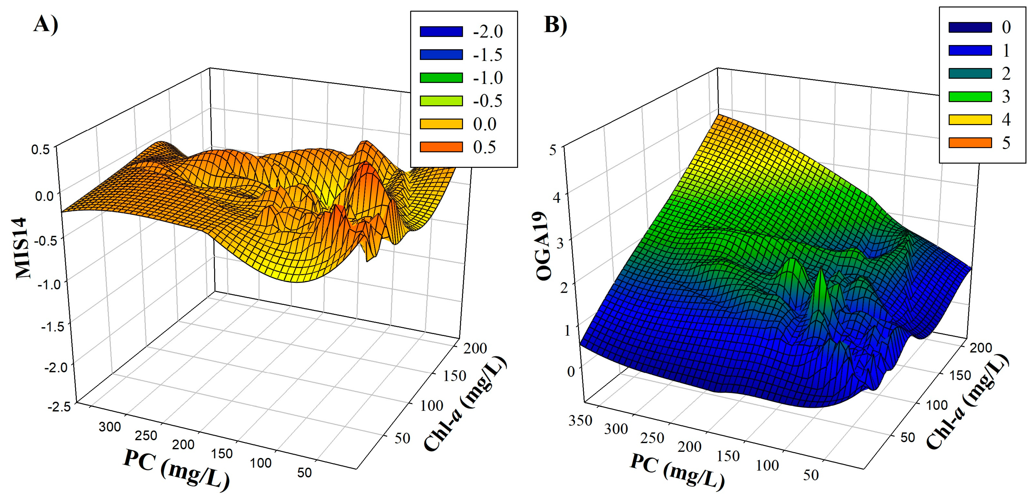
Although the MIS14 algorithm resulted in a lower RMSE and MAE than OGA19 when applied to the 2010 MR validation dataset, a sensitivity analysis of OGA19 and MIS14 confirmed the advantage of the former than the latter when applied to all MR datasets. Shown in Figure 7 are three-dimensional plots with chl-a and PC concentrations being axes Y and X and algorithm values being axis Z. It is obvious that the three-dimensional plot for MIS14 does not show a linear relationship between the algorithm value and PC concentrations as chl-a concentration varies (Figure 7A). In contrast, a strong linear relationship between the OGA19 value and PC concentration is evident with increasing chl-a concentration (Figure 7B). This sensitivity analysis suggests that the proposed OGA 19 is less sensitive to chl-a than the MIS14 algorithm and should be favorable for retrieval of PC concentrations from remote sensing data.
OGA19 was also compared to the semi-analytical algorithm: SIM05 (Figure 5 and Figure 6). The tuning results suggest similar performances between SIM05 and OGA19 (Figure 5). For each yearly dataset of a given study site, OGA19 performed slightly better than SIM05, but the biggest difference was for the ECR 2007 dataset with the R2 value for OGA19 being 0.85 as opposed to 0.16 for SIM05. For the validation result (Figure 6) the performances from both algorithms were similar though OGA19 resulted in slightly lower RMSE and MAE values than SIM05 did with the exception of GR for which SIM05 got a lower MAE. In spite of their similar performance, OGA19 has the advantages over SIM05 because OGA19 is simple Equation (14) as compared with SIM05 which needs to calculate parameters such as aw(709), aw(665), bb, ϒ, δ and ε (Equations (16) and (17)).
OGA19 has been shown to outperform several semi-empirical and semi-analytical algorithms. Recent reviews on this topic have shown that a simple algorithm like band ratios generated accurate estimates [20,29,33,34]. In this study, the ratio between the Rrs at 709 nm and 620 nm was used to approximate the aphy at 620 nm (Figure 1). Based on the high R2 value 0.9, it is worth comparing the use of OGA19 with the band ratio between 709 and 620 nm for the estimation of PC. Table 8 shows that the OGA19 performed better when tuned against all year datasets collected from each of the three central Indiana Reservoirs. For ECR, OGA19 got an R2 of 0.67 while the band ratio got an R2 of 0.50; for MR the proposed algorithm got an R2 of 0.65 which is higher than 0.52 obtained by the band ratio; for GR, both algorithms showed a poor performance with R2 values of 0.20 and 0.18 for OGA19 and the band ratio, respectively.
Poor performance of both algorithms for GR was also observed for SIM05 (Figure 5), HUN08, MIS14, and LIU17(Table 3), meaning that none of these remote sensing algorithms provided accurate estimates of PC for GR and this needs further explanation.
Hunter et al. [41] showed that the increase of sediments in the water column can enhance the prominence of the chl-a and PC absorption features and result in a shift in the Rrs spectra. The Rrs spectra of the GR 2006 dataset were observed to shift to approximately 680 nm for the chl-a absorption feature and to approximately 635 nm for the PC absorption feature. Therefore, it is believed that high turbidity caused by dredging GR affected spectral estimation of PC. In the 2005 dataset for GR, the average TSS concentration was 15.79 mg/L. However, with the dredging started in 2006, the average TSS was 17.40 mg/L in 2006 and 23.55 mg/L in 2007, indicating an increased TSS concentration from 2005 to 2007. Given that phytoplankton concentration was part of TSS in this study, the ratio of chl-a concentration (µg/L) and TSS concentration (mg/L) was computed for these datasets to determine the relative dominance of phytoplankton and TSS. The ratio was 0.89, 4.25, and 6.32 µg/mg for years 2005, 2006, and 2007, respectively, suggesting that dredging the reservoirs led to an increase in chl-a concentration as a result of the resuspension of nutrients trapped in the sediment. Based on the observation that changing the spectral bands used in the formulation of OGA19 in the 2006 dataset resulted in improved PC estimates with R2 being 0.43, we conclude that a high sediment load in the water column led to shifted absorption features and resulted in the poor performance of all algorithms when applied to the 2006 GR dataset. However, errors in the sample collection and the process of analyzing PC concentration cannot be ruled out.
Both the band ratio algorithm and OGA19 were validated on the 2010 datasets for the three central Indiana study sites. Figure 8 shows the scatterplots for measured and remotely estimated PC for ECR (Figure 8A), GR (Figure 8B), and MR (Figure 8C). OGA19 outperformed the band ratio with a lower RMSE and MAE for ECR and GR (Table 9); however, for MR, the band ratio algorithm got a lower RMSE and MAE than OGA19. This relative weak performance of OGA19 for MR was similar to the case that MIS14 resulted in a lower RMSE and MAE than OGA19 did.
To get insights into these results, we examined the PC:chl-a ratio of the samples (Table 1). It was observed that OGA19 presented a stronger relationship for ECR in which chl-a dominated over PC (mean PC:chl-a = 0.95), and for GR where PC concentrations were marginally higher than chl-a (mean PC:chl-a = 1.17). On the other hand, the MR dataset presented PC concentration higher than chl-a concentration (mean PC:chl-a = 1.31) for which MIS14 achieved the lowest RMSE value. These results indicate that OGA19 performed strongly at a low (e.g., ECR) or intermediate (e.g., GR) PC:chl-a ratio. However for the case of a high PC:chl-a ratio (e.g., MR), OGA19 did not perform as well as MIS14 (Table 3) or the band ratio (Table 8).
We know that the absorption of phytoplankton is apparently not synonymous with the combination of computed absorption of isolated pigments. A complete compensation for the effect of phytoplankton pigments (other than chl-a) on the absorption at 620 nm was not possible in this study, but the fact that OGA19 performed well on the datasets collected for the three different study sites in different years indicates that OGA19 was not prone to the effect of other pigments as compared with other remote sensing algorithms. This analysis suggests that OGA19, which was developed to remove the chl-a interference on remote estimation of PC, overestimates the interference of chl-a when PC concentrations are high causing an underestimation in the PC concentration (Figure 4 and Figure 8). This occurs due to the structure of the algorithm Equation (14) in which the estimation of PC is done by subtraction of the chl-a influence at 620 nm. When PC is higher than chl-a, the presence of chl-a at 620 nm can be negligible and the correction for the chl-a influence is not needed. Therefore, MIS14 and the band ratio gave rise to a lower RMSE and MAE than OGA19 for the validation dataset as opposed to the tuning results. These results corroborate with the idea that the variation of PC:chl-a is an important factor influencing the performance of the remote sensing algorithm [12]. It is important to highlight that OGA19 performed better at low and medium PC:chl-a levels, and can be more applicable for early warning of cyanobacterial blooms because most of the algorithms do not perform well at low PC concentrations [26].
4.2. Pigment Package Effect on OGA19
The proposed algorithm was validated with pigment extracts (without the package effect) while remote sensing data were commonly collected for natural waters samples (with package effect). Unfortunately, to our knowledge, there are not studies investigating the package effect for each single pigment (PC and chl-a), only the absorption of phytoplankton was evaluated. Thus, to investigate the package effect influence on the OGA19 algorithm, we applied the coefficients proposed by Simis et al. [9] for aphy at 620 and 665 nm in Equation (14). Table 10 summarizes the regression and R2 values as well as the F-test which show the variance between the modeling results with and without correcting for the package effect.
It was observed that the difference was not significant between the values with and without the package effect correction. Although our results showed that the application of the coefficients proposed by Simis et al. [9] did not significantly improve the performance of OGA19, it is important to address the package effect on inland water phytoplankton and on each pigment. Recently, Alcantara et al. [47] showed that at higher chl-a concentrations the package effect is stronger, but they did not describe the difference between package and non-package samples. Therefore, studies are needed to further understand the package effect of inland water phytoplankton, especially in cyanobacteria.
4.3. Comparison between OGA19 and SIM05 based on Different achl-a (620) Values
In this study we proposed a new method for calculating the aPC (620) based on the computation of the achl-a at 620 nm and aPC at 665 nm (Equation (8) and (9)). Simis et al. [9] proposed the calculation of achl-a at 620 nm and assigned 0.24 as the value of ε. In this study, we used 0.2215 to relate achl-a at 665 nm to achl-a at 620 nm (Figure 2A). To evaluate if this value was appropriate, we compared the sensitivity to both φ1 = 0.2215 and ε = 0.24 of SIM05 and OGA19, respectively. Table 11 summarizes the results of R2 of this comparison.
The results presented in Table 11 show that when applied to the eight datasets, OGA19 with φ1 = 0.2215 had the best performance for five of them, and with φ1 = 0.24 got the best performance for two datasets, but SIM05 got the best performance only for one dataset. It was observed that SIM05 was improved on five datasets when ε was set to be 0.2215. On the contrary, OGA19 had a degraded performance in five datasets when φ1 was set to be 0.24. The most significant improvement was observed for the 2007 ECR dataset for which the original SIM05 got an R2 of 0.16 and an RMSE of 20.70 µg/L while the SIM05 with ε being 0.2215 got R2 and RMSE values of 0.34 and 20.06 µg/L respectively. Except for this dataset, the difference between SIM05 and OGA19 on other datasets was not significant. Therefore, the value that is used to relate achl-a at 665 nm to achl-a at 620 nm is not a major contributor to the different performances of SIM05 and OGA19.
5. Conclusions
A new remote sensing algorithm (OGA19) for the remote estimation of PC was introduced and compared to other semi-empirical, semi-analytical algorithms, and a simple band ratio. The newly developed remote sensing algorithm was evaluated using proximal (total of 544 sampling points) from three central Indiana reservoirs. OGA19 outperformed the selected semi-empirical algorithms and the simple band ratio for PC estimation and performed slightly better than the most widely cited SIM05 algorithm. Additionally, OGA19 showed little influence from the package effect, however, more studies are needed to fully understand the package effect of cyanobacteria cells. Considering OGA19’s simple computational structure and its consistent strong performance on the datasets collected in different time periods and sites, OGA19 could be used for operational monitoring of inland water quality [33].
Moreover, with the launch of satellites boarded with sensors that have a 620 nm spectral band, the use of satellites for monitoring cyanobacteria becomes feasible. One example of this sensor is the OLCI onboard at the recently launched Sentinel-3 from the European Space Agency (ESA). With the growing concern about inland waters, especially with the concerns related to human and environmental health, environmental programs have been taking the advantages of remote sensing technology to improve their spatial and temporal coverage. Thus, the present research provides a tool which can be used for temporal and spatial analysis to promote water governance.
Overall, we presented a new semi-empirical remote sensing algorithm capable of estimating PC better than other semi-empirical algorithms. The model was evaluated for different concentrations of PC and chl-a as well as their ratio. Moreover, we also emphasize the need for more studies about the sensitivity evaluation of remote sensing algorithms, especially because a sensitivity analysis is important to detect the malfunctions on the algorithm structure.
Author Contributions
Conceptualization, I.O. and L.L.; Formal analysis, I.O.; Project administration, L.L.; Supervision, L.L.; Visualization, I.O.; Writing—original draft, I.O.; Writing—review & editing, I.O. and L.L.
Funding
This research was funded by NASA Energy and Water Cycle Study program, grant number NNX09AU87G and Indiana University Collaborative Research Grants program (IUCRG). The APC was funded by the Indiana University – Purdue University at Indianapolis (IUPUI) Open Access Fund.
Acknowledgments
Authors thank staff from the Center of Earth and Environmental Sciences (CEES) located at Indiana University–Purdue University Indianapolis (IUPUI), and graduate students and postdocs of the Planetary and Environmental Remote Sensing Laboratory (PERSL) for helping with water samples analysis and in situ spectral measurement. Authors also would like to thank the funding support by the NASA Energy and Water Cycle Study program (grant no. NNX09AU87G), Veolia Waters, and Indiana University Collaborative Research Grants program (IUCRG).
Conflicts of Interest
The authors declare no conflict of interest.
References
- Codd, G.A.; Lindsay, J.; Young, F.M.; Morrison, L.F.; Metcalf, J.S. Harmful Cyanobacteria. In Harmful Cyanobacteria, 1st ed.; Huisman, J., Matthijs, H.C.P., Visser, P.M., Eds.; Springer: Dordrecht, The Netherlands, 2005; pp. 1–23. [Google Scholar]
- Reynolds, C.S. Cyanobacterial water blooms. In Advances in Botanical Research; Callow, J.A., Ed.; Academic Press: London, UK, 1987; pp. 67–143. [Google Scholar]
- Hyenstrand, P.; Blomqvist, P.; Pettersson, A. Factors determining cyanobacterial success in aquatic systems: A literature review. Arch. Hydrobiol. 1998, 51, 41–62. [Google Scholar]
- Paerl, H.W. Marine Plankton. In Ecology of Cyanobacteria II: Their Diversity in Space and Time; Whitton, B.A., Ed.; Springer: Dordrecht, The Netherlands, 2012; pp. 127–153. [Google Scholar]
- Sivonen, K.; Jones, G. Cyanobacterial Toxins. In Toxic Cyanobacteria in Water: A Guide to Their Public Health Consequences, Monitoring and Management, 1st ed.; Chorus, I., Bartram, J., Eds.; UNESCO/WHO/UNEP: London, UK, 1999; pp. 55–124. [Google Scholar]
- Carmichael, W.W. Health effects of toxin producing cyanobacteria: The cyanoHABs. Hum. Ecol. Risk Assess. 2001, 7, 1393–1407. [Google Scholar] [CrossRef]
- Duan, H.; Ma, R.; Xu, J.; Zhang, Y.; Zhang, B. Comparison of different semi-empirical algorithms to estimate chlorophyll-a concentration in inland lake water. Environ. Monit. Assess. 2010, 170, 231–244. [Google Scholar] [CrossRef] [PubMed]
- Gons, H.J. Optical teledetection of chlorophyll-a in turbid inland waters. Environ. Sci. Technol. 1999, 33, 1127–1132. [Google Scholar] [CrossRef]
- Simis, S.G.H.; Peters, S.W.M.; Gons, H.J. Remote sensing of the cyanobacterial pigment phycocyanin in turbid inland water. Limnol. Oceanogr. 2005, 50, 237–245. [Google Scholar] [CrossRef]
- Li, L.; Sengpiel, R.E.; Pascual, D.L.; Tedesco, L.D.; Wilson, J.S.; Soyeux, E. Using hyperspectral remote sensing to estimate chlorophyll-a and phycocyanin in a mesotrophic reservoir. Int. J. Remote. Sens. 2010, 31, 4147–4162. [Google Scholar] [CrossRef]
- Le, C.; Li, Y.; Zha, Y.; Wang, Q.; Zhang, H.; Yin, B. Remote sensing of phycocyanin pigment in highly turbid inland waters in Lake Taihu, China. Int. J. Remote Sens. 2011, 32, 8253–8269. [Google Scholar] [CrossRef]
- Li, L.; Li, L.; Shi, K.; Li, Z.; Song, K. A semi-analytical algorithm for remote estimation of phycocyanin in inland waters. Sci. Total Environ. 2012, 435-436, 141–150. [Google Scholar] [CrossRef]
- Song, K.; Li, L.; Li, Z.; Tedesco, L.; Hall, B.; Shi, K. Remote detection of cyanobacteria through phycocyanin for water supply source using three-band model. Ecol. Inform. 2013, 15, 22–33. [Google Scholar] [CrossRef]
- Li, L.; Li, L.; Song, K. Remote sensing of freshwater cyanobacteria: An extended IOP Inversion Model of Inland Waters (IIMIW) for partitioning absorption coefficient and estimating phycocyanin. Remote Sens. Environ. 2015, 157, 9–23. [Google Scholar] [CrossRef]
- Matthews, M.W.; Odermatt, D. Improved algorithm for routine monitoring of cyanobacteria and eutrophication in inland and near-coastal waters. Remote Sens. Environ. 2015, 156, 374–382. [Google Scholar] [CrossRef]
- Reinart, A.; Kutser, T. Comparison of different satellite sensors in detecting cyanobacterial bloom events in the Baltic Sea. Remote Sens. Environ. 2006, 102, 74–85. [Google Scholar] [CrossRef]
- Hunter, P.D.; Tyler, A.N.; Gilvear, D.J.; Willby, N.J. Using remote sensing to aid the assessment of human health risks from blooms of potentially toxic cyanobacteria. Environ. Sci. Technol. 2009, 43, 2627–2633. [Google Scholar] [CrossRef] [PubMed]
- Vincent, R.K.; Qin, X.M.; McKay, R.M.L.; Miner, J.; Czajkowski, K.; Savino, J.; Bridgeman, T. Phycocyanin detection from LANDSAT TM data for mapping cyanobacterial blooms in Lake Erie. Remote Sens. Environ. 2004, 89, 381–392. [Google Scholar] [CrossRef]
- Mishra, S.; Mishra, D.R.; Schluchter, W.M. A novel algorithm for predicting phycocyanin concentrations in cyanobacteria: A proximal hyperspectral remote sensing approach. Remote Sens. 2009, 1, 758–775. [Google Scholar] [CrossRef]
- Ogashawara, I.; Mishra, D.R.; Mishra, S.; Curtarelli, M.P.; Stech, J.L. A performance review of reflectance based algorithms for predicting phycocyanin concentrations in inland waters. Remote Sens. 2013, 5, 4774–4798. [Google Scholar] [CrossRef]
- Dekker, A.G. Detection of Optical Water Quality Parameters for Eutrophic Waters by High Resolution Remote Sensing. Ph.D. Thesis, Vrije Universiteit, Amsterdam, The Netherlands, 1993. [Google Scholar]
- Schalles, J.F.; Yacobi, Y.Z. Remote detection and seasonal patterns of phycocyanin, carotenoid, and chlorophyll pigments in eutrophic waters. Arch. Hydrobiol. 2000, 55, 153–168. [Google Scholar]
- Metsamaa, L.; Kutser, T.; Strombeck, N. Recognising cyanobacterial blooms based on their optical signature: A modeling study. Boreal Environ. Res. 2006, 11, 493–506. [Google Scholar]
- Ogashawara, I. Terminology and classification of bio-optical algorithms. Remote Sens. Lett. 2015, 6, 613–617. [Google Scholar] [CrossRef]
- Mishra, S.; Mishra, D.R.; Lee, Z.; Tucker, C.S. Quantifying cyanobacterial phycocyanin concentration in turbid productive waters: A quasi-analytical approach. Remote Sens. Environ. 2013, 133, 141–151. [Google Scholar] [CrossRef]
- Ruiz-Verdu, A.; Simis, S.G.H.; de Hoyos, C.; Gons, H.J.; Pena-Martinez, R. An evaluation of algorithms for the remote sensing of cyanobacterial biomass. Remote Sens. Environ. 2008, 112, 3996–4008. [Google Scholar] [CrossRef]
- Yan, Y.; Bao, Z.; Shao, J. Phycocyanin concentration retrieval in inland waters: A comparative review of the remote sensing techniques and algorithms. J. Great Lakes Res. 2018, 44, 748–755. [Google Scholar] [CrossRef]
- Mishra, S.; Mishra, D.R.; Lee, Z. Bio-optical inversion in highly turbid and cyanobacteria dominated waters. IEEE Trans. Geosci. Remote Sens. 2014, 52, 375–388. [Google Scholar] [CrossRef]
- Mouw, C.B.; Greb, S.; Aurin, D.; DiGiacomo, P.M.; Lee, Z.; Twardowski, M.; Binding, C.; Hu, C.; Ma, R.; Moore, T.; et al. Aquatic color radiometry remote sensing of coastal and inland waters: Challenges and recommendations for future satellite missions. Remote Sens. Environ. 2015, 160, 15–30. [Google Scholar] [CrossRef]
- Gordon, H.R.; Brown, O.B.; Jacobs, M.M. Computed relationships between the inherent and apparent optical properties of a flat homogeneous ocean. Appl. Opt. 1975, 14, 417–427. [Google Scholar] [CrossRef] [PubMed]
- Gordon, H.R.; Brown, O.B.; Evans, R.H.; Brown, J.W.; Smith, R.C.; Baker, K.S.; Clark, D.K. A Semianalytic radiance model of ocean color. J. Geophys. Res. 1988, 93, 10909–10924. [Google Scholar] [CrossRef]
- Kirk, J.T.O. Light and Phytosynthesis in Aquatic Ecosystems, 2nd ed.; Cambridge Univ. Press: New York, NY, USA, 1994. [Google Scholar]
- Augusto-Silva, P.B.; Ogashawara, I.; Barbosa, C.C.F.; de Carvalho, L.A.S.; Jorge, D.S.F.; Fornari, C.I.; Stech, J.L. Analysis of MERIS reflectance algorithms for estimating chlorophyll-a concentration in a Brazilian Reservoir. Remote Sens. 2014, 6, 11689–11707. [Google Scholar] [CrossRef]
- Gurlin, D.; Gitelson, A.A.; Moses, W.J. Remote estimation of chl-a concentration in turbid productive waters —Return to a simple two-band NIR-red model? Remote Sens. Environ. 2011, 115, 3479–3490. [Google Scholar] [CrossRef]
- Beck, R.; Zhan, S.; Liu, H.; Tong, S.; Yang, B.; Xu, M.; Ye, Z.; Huang, Y.; Shu, S.; Wu, Q.; et al. Comparison of satellite reflectance algorithms for estimating chlorophyll-a in a temperate reservoir using coincident hyperspectral aircraft imagery and dense coincident surface observations. Remote Sens. Environ. 2016, 178, 15–30. [Google Scholar] [CrossRef] [Green Version]
- Werdell, P.J.; Bailey, S.; Fargion, G.; Pietras, C.; Knobelspiesse, K.; Feldman, G.; McClain, C. Unique data repository facilitates ocean color satellite validation. EOS Trans. AGU 2003, 84, 379. [Google Scholar] [CrossRef]
- Werdell, P.J.; Baily, S.W. An improved in situ bio-optical data set for ocean color algorithm development and satellite data product validation. Remote Sens. Environ. 2005, 98, 122–140. [Google Scholar] [CrossRef]
- Marra, J.; Trees, C.C.; O’Reilly, J.E. Phytoplankton Pigment Absorption: A Strong Predictor of Primary Productivity in the Surface Ocean. Deep Sea Res. Part 1 Oceanogr. Res. Pap. 2007, 54, 155–163. [Google Scholar] [CrossRef]
- Gitelson, A.A.; Schalles, J.F.; Hladik, C.M. Remote chlorophyll-a retrieval in turbid, productive estuaries: Chesapeake Bay case study. Remote Sens. Environ. 2007, 109, 464–472. [Google Scholar] [CrossRef]
- Ritchie, R.J. Universal chlorophyll equations for estimating chlorophylls a, b, c, and d and total chlorophylls in natural assemblages of photosynthetic organisms using acetone, methanol, or ethanol solvents. Photosynthetica 2008, 46, 115–126. [Google Scholar] [CrossRef]
- Hunter, P.D.; Tyler, A.N.; Présing, M.; Kovács, A.W.; Preston, T. Spectral discrimination of phytoplankton colour groups: The effect of suspended particulate matter and sensor spectral resolution. Remote Sens. Environ. 2008, 112, 1527–1544. [Google Scholar] [CrossRef]
- Mishra, S.; Mishra, D.R. A novel remote sensing algorithm to quantify phycocyanin in cyanobacterial algal blooms. Environ. Res. Lett. 2014, 9, 114003. [Google Scholar] [CrossRef]
- Liu, G.; Simis, S.G.H.; Li, L.; Wang, Q.; Li, Y.; Song, K.; Lyu, H.; Zheng, Z.; Shi, K. A four-band semi-analytical model for estimating phycocyanin in inland waters from simulated MERIS and OLCI data. IEEE Trans. Geosci. Remote Sens. 2017, 56, 1374–1385. [Google Scholar] [CrossRef]
- Gitelson, A. The peak near 700 nm on radiance spectra of algae and water: Relationships of its magnitude and position with chlorophyll concentration. Int. J. Remote Sens. 1992, 13, 3367–3373. [Google Scholar] [CrossRef]
- Dall’Olmo, G.; Gitelson, A.A. Effect of bio-optical parameter variability on the remote estimation of chlorophyll-a concentration in turbid productive waters: Experimental results. Appl. Opt. 2005, 44, 412–422. [Google Scholar] [CrossRef] [PubMed]
- Guanter, L.; Ruiz-Verdu, A.; Odermatt, D.; Giardino, C.; Simis, S.; Estelles, V.; Heegeg, T.; Domínguez-Gómez, J.A.; Moreno, J. Atmospheric correction of ENVISAT/MERIS data over inland waters: Validation for European lakes. Remote Sens. Environ. 2010, 114, 467–480. [Google Scholar] [CrossRef] [Green Version]
- Alcantara, E.; Watanabe, F.; Rodrigues, T.; Bernado, N. An investigation into the phytoplankton package effect on the chlorophyll-a specific absorption coefficient in Barra Bonita reservoir, Brazil. Remote Sens. Lett. 2018, 7, 761–770. [Google Scholar] [CrossRef]
Figure 1.
Linear relationship between aphy at 665 nm and Rrs 709/665 (A), and between aphy at 620 nm and Rrs 709/620 (B).
Figure 1.
Linear relationship between aphy at 665 nm and Rrs 709/665 (A), and between aphy at 620 nm and Rrs 709/620 (B).

Figure 2.
Linear relationships between the absorption coefficients at 620 and 665 nm measured for Sigma Aldrich standards: Chl-a (A) and PC (B).
Figure 2.
Linear relationships between the absorption coefficients at 620 and 665 nm measured for Sigma Aldrich standards: Chl-a (A) and PC (B).

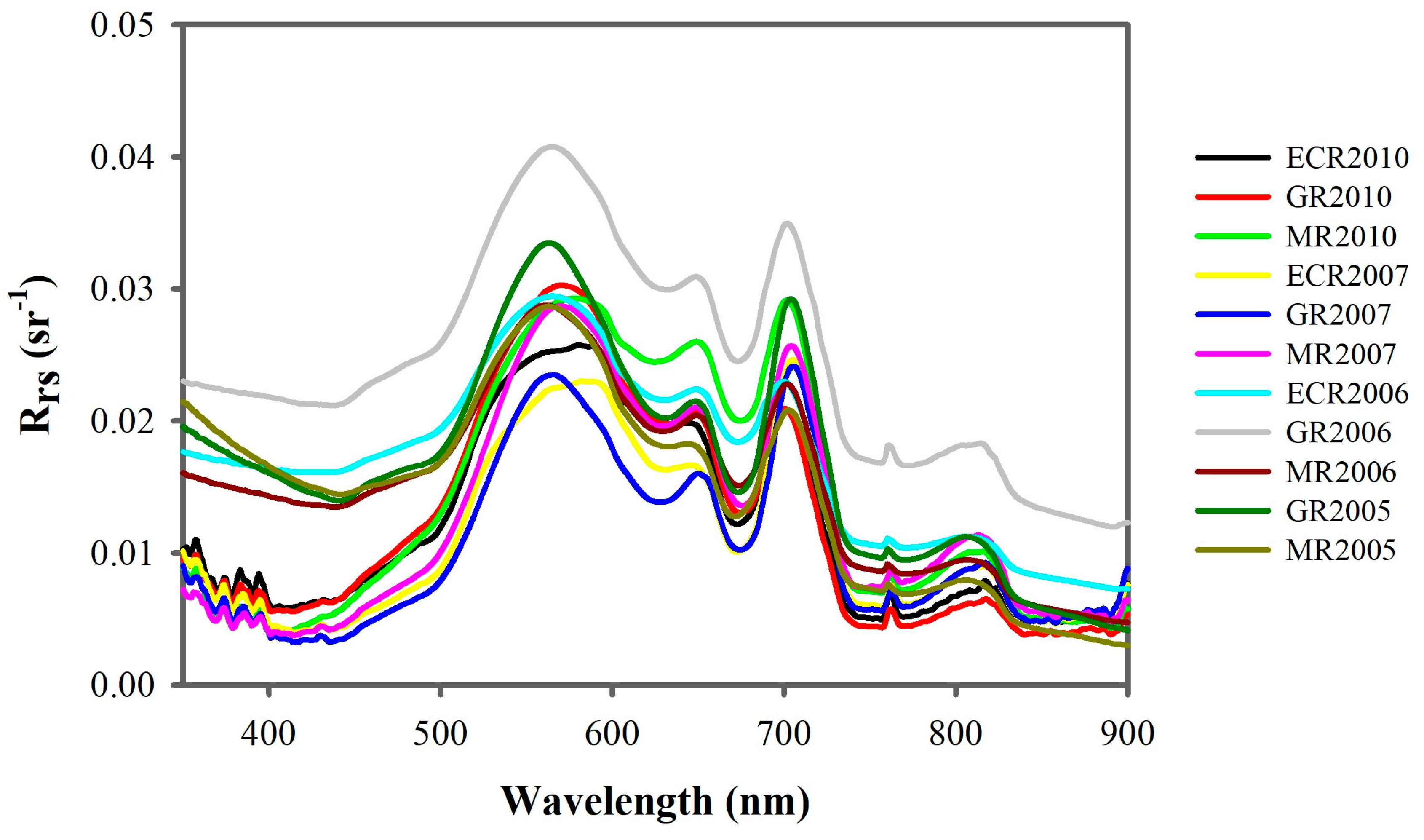
Figure 3.
Average Rrs (sr−1) spectra for each dataset.

Figure 4.
Validation of the semi-empirical algorithms using 2010 datasets for ECR (A), GR (B), and MR (C).
Figure 4.
Validation of the semi-empirical algorithms using 2010 datasets for ECR (A), GR (B), and MR (C).

Figure 5.
Tuning results for SIM05 (left) and OGA19 (right) using 2005–2007 datasets for ECR (A,B), GR (C,D) and MR (E,F).
Figure 5.
Tuning results for SIM05 (left) and OGA19 (right) using 2005–2007 datasets for ECR (A,B), GR (C,D) and MR (E,F).

Figure 6.
Validation results for SIM05 and OGA19 using the 2010 datasets of ECR (A), GR (B), and MR (C).
Figure 6.
Validation results for SIM05 and OGA19 using the 2010 datasets of ECR (A), GR (B), and MR (C).

Figure 7.
Sensitivity analysis of MIS14 (A) and OGA19 (B) when applied to the MR data collected in years 2005–2007 and 2010.
Figure 7.
Sensitivity analysis of MIS14 (A) and OGA19 (B) when applied to the MR data collected in years 2005–2007 and 2010.

Figure 8.
Validation results for the band ratio (BR) and OGA19 algorithms using the 2010 datasets of ECR (A), GR (B), and MR (C).
Figure 8.
Validation results for the band ratio (BR) and OGA19 algorithms using the 2010 datasets of ECR (A), GR (B), and MR (C).


Table 1.
Semi-empirical algorithms for remote estimation of PC.
| Acronym | Formulation | References |
|---|---|---|
| HUN08 | * | [41] |
| MIS14 | [42] | |
| LIU17 | [43] |
* Adjusted for MERIS/OLCI spectral bands.
Table 2.
Limnological variables for central Indiana reservoirs ECR, GR, and MR.
| ECR | GR | MR | |||||||
|---|---|---|---|---|---|---|---|---|---|
| Chl-a (µg/L) | PC (µg/L) | TSS (mg/L) | Chl-a (µg/L) | PC (µg/L) | TSS (mg/L) | Chl-a (µg/L) | PC (µg/L) | TSS (mg/L) | |
| Mean | 53.54 | 51.29 | 13.65 | 70.44 | 82.58 | 17.02 | 58.64 | 75.46 | 16.37 |
| Median | 40.14 | 31.46 | 12.25 | 61.70 | 77.49 | 15.56 | 51.63 | 57.94 | 13.96 |
| Minimum | 2.93 | 0.73 | 3.14 | 14.45 | 0.91 | 6.30 | 1.85 | 1.39 | 3.85 |
| Maximum | 255.00 | 234.28 | 38.24 | 193.18 | 210.20 | 81.17 | 214.20 | 370.95 | 123.79 |
Table 3.
Coefficients of Determination for semi-empirical PC estimation algorithms calibrated on the 2005–2007 datasets. Best performances are highlighted in bold.
Table 3.
Coefficients of Determination for semi-empirical PC estimation algorithms calibrated on the 2005–2007 datasets. Best performances are highlighted in bold.
| Year | Reservoir | HUN08 | MIS14 | LIU17 | OGA19 |
|---|---|---|---|---|---|
| 2006 | ECR (n = 84) | R2 < 0.01 | R2 = 0.17 | R2 = 0.39 | R2 = 0.81 |
| 2007 | ECR (n = 22) | R2 = 0.32 | R2 = 0.41 | R2 = 0.21 | R2 = 0.85 |
| 2005 | GR (n = 27) | R2 < 0.01 | R2 = 0.35 | R2 = 0.46 | R2 = 0.68 |
| 2006 | GR (n = 86) | R2 < 0.01 | R2 = 0.04 | R2 = 0.15 | R2 = 0.38 |
| 2007 | GR (n = 16) | R2 = 0.14 | R2 = 0.70 | R2 = 0.48 | R2 = 0.93 |
| 2005 | MR (n = 23) | R2 = 0.63 | R2 = 0.61 | R2 = 0.35 | R2 = 0.91 |
| 2006 | MR (n = 85) | R2 = 0.36 | R2 < 0.01 | R2 = 0.66 | R2 = 0.76 |
| 2007 | MR (n = 16) | R2 = 0.47 | R2 = 0.67 | R2 = 0.22 | R2 = 0.77 |
Table 4.
Algorithm’s coefficients resulting from tuning.
| ECR | GR | MR | ||||
|---|---|---|---|---|---|---|
| Slope | Intercept | Slope | Intercept | Slope | Intercept | |
| HUN08 | −87.194 | 52.725 | −165 | 68.823 | 228.14 | 101.19 |
| MIS14 | −76.307 | 47.651 | −111.45 | 62.555 | −30.935 | 72.901 |
| LIU17 | 53.445 | 62.866 | 703.77 | 87.124 | 710.13 | 80.615 |
| OGA19 | 165.89 | −127.05 | 57.92 | 7.2021 | 167.91 | −123.04 |
Table 5.
Comparison of error metrics among different semi-empirical algorithms.
| ECR | GR | MR | ||||
|---|---|---|---|---|---|---|
| MAE | RMSE | MAE | RMSE | MAE | RMSE | |
| HUN08 | 34.511 | 20.381 | 44.302 | 34.498 | 51.247 | 31.576 |
| MIS14 | 35.128 | 21.466 | 42.825 | 45.070 | 35.529 | 20.051 |
| LIU17 | 28.218 | 18.427 | 31.530 | 27.564 | 48.980 | 45.616 |
| OGA19 | 15.168 | 14.439 | 29.935 | 18.609 | 40.858 | 23.004 |
Table 6.
Comparison of error metrics between SIM05 and OGA19.
| ECR | GR | MR | ||||
|---|---|---|---|---|---|---|
| MAE | RMSE | MAE | RMSE | MAE | RMSE | |
| SIM05 | 20.204 | 15.856 | 25.415 | 19.603 | 42.096 | 23.658 |
| OGA19 | 15.168 | 14.439 | 29.935 | 18.609 | 40.858 | 23.004 |
Table 7.
Calibration for SIM05 and OGA19 using simulated OLCI spectra.
| Year | Reservoir | SIM05 | OGA19 | SIM05 with φ1 | OGA19 with ε |
|---|---|---|---|---|---|
| 2006 | ECR (n = 84) | R2 = 0.80 | R2 = 0.80 | R2 = 0.80 | R2 = 0.80 |
| 2007 | ECR (n = 22) | R2 = 0.24 | R2 = 0.85 | R2 = 0.45 | R2 = 0.86 |
| 2005 | GR (n = 27) | R2 =0.69 | R2 = 0.68 | R2 = 0.69 | R2 = 0.68 |
| 2006 | GR (n = 86) | R2 =0.37 | R2 = 0.38 | R2 = 0.37 | R2 = 0.38 |
| 2007 | GR (n = 16) | R2 = 0.82 | R2 = 0.93 | R2 = 0.85 | R2 = 0.93 |
| 2005 | MR (n = 23) | R2 = 0.88 | R2 = 0.91 | R2 = 0.89 | R2 = 0.91 |
| 2006 | MR (n = 85) | R2 = 0.74 | R2 = 0.76 | R2 =0.73 | R2 = 0.77 |
| 2007 | MR (n = 16) | R2 = 0.73 | R2 = 0.77 | R2 = 0.75 | R2 = 0.77 |
Table 8.
Tuned models for OGA19 and Band Ratio (709/620), values in bold indicate the highest R2.
| ECR (2006–2007) | GR (2005–2007) | MR (2005–2007) | |
|---|---|---|---|
| OGA19 | y = 165.89x − 127.05 R2 = 0.6793 | y = 57.92x + 7.2021 R2 = 0.2012 | y = 167.91x − 123.04 R2 = 0.6503 |
| Band Ratio (709/620) | y = 128.58x − 75.63 R2 = 0.504 | y = 61.01x + 9.6893 R2 = 0.1843 | y = 166.35x − 106.36 R2 = 0.5247 |
Table 9.
Error’s estimators for the comparison between BR and OGA19.
| ECR | GR | MR | ||||
|---|---|---|---|---|---|---|
| MAE | RMSE | MAE | RMSE | MAE | RMSE | |
| BR | 17.913 | 20.06 | 32.211 | 21.13 | 39.805 | 19.73 |
| OGA19 | 15.168 | 14.439 | 29.935 | 18.609 | 40.858 | 23.004 |
Table 10.
Comparison between OGA19 performances with and without the package effect correction for all datasets.
Table 10.
Comparison between OGA19 performances with and without the package effect correction for all datasets.
| Datasets | OGA19 | OGA19 − Package Effect | F-Test | Statistical Difference |
|---|---|---|---|---|
| ECR 2006 | y = 220.16x − 178.42 R2 = 0.8104 | y = 197.91x − 174.03 R2 = 0.7999 | F = 1.221 p = 0.36 | No |
| ECR 2007 | y = 76.787x − 31.005 R2 = 0.8558 | y = 82.362x − 42.813 R2 = 0.8624 | F = 1.141 p = 0.76 | No |
| ECR2010 | y = 96.316x − 61.383 R2 = 0.5647 | y = 91.725x − 54.992 R2 = 0.4646 | F = 1.102 p=0.70 | No |
| GR2005 | y = 147.85x − 121.93 R2 = 0.6802 | y = 133.07x − 115.63 R2 = 0.6872 | F = 1.247 p = 0.57 | No |
| GR2006 | y = 256.07x − 224.69 R2 = 0.3824 | y = 224.73x − 210.88 R2 = 0.3783 | F = 1.284 p = 0.25 | No |
| GR2007 | y = 84.39x − 85.562 R2 = 0.9312 | y = 76.52x − 83.09 R2 = 0.9248 | F = 1.207 p = 0.71 | No |
| GR2010 | y = 174.76x − 147.56 R2 = 0.834 | y = 188.38x − 154.84 R2 = 0.8262 | F = 1.172 p = 0.63 | No |
| MR2005 | y = 106.24x − 67.876 R2 = 0.9158 | y = 99.283x − 67.687 R2 = 0.9128 | F = 1.141 p = 0.75 | No |
| MR2006 | y = 236.45x − 202.87 R2 = 0.7686 | y = 210.96x − 195.43 R2 = 0.7858 | F = 1.284 p = 0.25 | No |
| MR2007 | y = 61.378x + 2.624 R2 = 0.7744 | y = 58.56x + 2.1764 R2 = 0.7722 | F = 1.095 p = 0.86 | No |
| MR2010 | y = 141.61x − 127.82 R2 = 0.7519 | y = 147.27x − 127.47 R2 = 0.7802 | F = 1.042 p = 0.88 | No |
Table 11.
Comparison of SIM05 and OGA19 for their sensitivity to φ1 and ε. Bold font indicates the best model performance for each dataset.
Table 11.
Comparison of SIM05 and OGA19 for their sensitivity to φ1 and ε. Bold font indicates the best model performance for each dataset.
| Year | Reservoir | SIM05 | OGA19 | SIM05 with φ1 | OGA19 with ε |
|---|---|---|---|---|---|
| 2006 | ECR (n = 84) | R2 = 0.80 | R2 = 0.81 | R2 = 0.80 | R2 = 0.80 |
| 2007 | ECR (n = 22) | R2 = 0.16 | R2 = 0.85 | R2 = 0.34 | R2 = 0.86 |
| 2005 | GR (n = 27) | R2 =0.69 | R2 = 0.68 | R2 = 0.69 | R2 = 0.68 |
| 2006 | GR (n = 86) | R2 =0.38 | R2 = 0.38 | R2 = 0.38 | R2 = 0.38 |
| 2007 | GR (n = 16) | R2 = 0.80 | R2 = 0.93 | R2 = 0.84 | R2 = 0.92 |
| 2005 | MR (n = 23) | R2 = 0.87 | R2 = 0.91 | R2 = 0.88 | R2 = 0.91 |
| 2006 | MR (n = 85) | R2 = 0.74 | R2 = 0.76 | R2 =0.73 | R2 = 0.77 |
| 2007 | MR (n = 16) | R2 = 0.72 | R2 = 0.77 | R2 = 0.64 | R2 = 0.77 |
© 2019 by the authors. Licensee MDPI, Basel, Switzerland. This article is an open access article distributed under the terms and conditions of the Creative Commons Attribution (CC BY) license (http://creativecommons.org/licenses/by/4.0/).
Share and Cite
MDPI and ACS Style
Ogashawara, I.; Li, L. Removal of Chlorophyll-a Spectral Interference for Improved Phycocyanin Estimation from Remote Sensing Reflectance. Remote Sens. 2019, 11, 1764. https://doi.org/10.3390/rs11151764
AMA Style
Ogashawara I, Li L. Removal of Chlorophyll-a Spectral Interference for Improved Phycocyanin Estimation from Remote Sensing Reflectance. Remote Sensing. 2019; 11(15):1764. https://doi.org/10.3390/rs11151764
Chicago/Turabian StyleOgashawara, Igor, and Lin Li. 2019. "Removal of Chlorophyll-a Spectral Interference for Improved Phycocyanin Estimation from Remote Sensing Reflectance" Remote Sensing 11, no. 15: 1764. https://doi.org/10.3390/rs11151764
Note that from the first issue of 2016, this journal uses article numbers instead of page numbers. See further details here.