A Simulation Environment for Validation and Verification of Real Time Hyperspectral Processing Algorithms on-Board a UAV

Abstract

The utilization of hyperspectral imaging sensors has gained a significant relevance among many different applications due to their capability for collecting a huge amount of information across the electromagnetic spectrum. These sensors have been traditionally mounted on-board satellites and airplanes in order to extract information from the Earth’s surface. Fortunately, the progressive miniaturization of these sensors during the last lustrum has enabled their use in other remote sensing platforms, such as drones equipped with hyperspectral cameras which bring advantages in terms of higher spatial resolution of the acquired images, more flexible revisit times and lower cost of the flight campaigns. However, when these drones are autonomously flying and taking real-time critical decisions from the information contained in the captured images, it is crucial that the whole process takes place in a safe and predictable manner. In order to deal with this problem, a simulation environment is presented in this work to analyze the virtual behavior of a drone equipped with a pushbroom hyperspectral camera used for assisting harvesting applications, which enables an exhaustive and realistic validation and verification of the drone real-time hyperspectral imaging system prior to its launch. To the best of the authors’ knowledge, the proposed environment represents the only solution in the state-of-the-art that allows the virtual verification of real-time hyperspectral image processing algorithms under realistic conditions.

1. Introduction

Hyperspectral imaging technology has gained momentum over the last years because of its capability for providing abundant spectral information that allows discover subtle differences of the scene that cannot be uncovered with other optical devices. Moreover, nowadays hyperspectral sensors have substantially reduced their sizes and have reached very competitive prices. This has led to the appearance of several applications in fields such as defense [1], security [2], mineral identification [3], and environmental protection [4], among others [5]. Alongside with the hyperspectral technology expansion, unmanned aerial vehicles (UAVs) have opened a new era in remote sensing, enabling the development of ad-hoc platforms at a much lower price, with some relevant advantages compared to satellites and airplanes. A flexible revisit time, enhanced spatial resolution and their capability of being controlled autonomously are some of the most important ones that make such platforms very appealing. Additionally, these platforms have the potential of performing missions that eventually provide results in real time, what makes them suitable for specific monitoring and surveillance applications that demand a prompt reaction to an stimulus. For all the mentioned reasons, the use of hyperspectral sensors on-board UAVs has gained widespread attention in the scientific community [6,7].

However, the use of such autonomous systems equipped with hyperspectral sensors poses a new challenge for researchers and developers, not only adapting the algorithm implementations to be able to work in real-time as images are being captured, but also making the appropriate modifications to let it coexist with the autonomous system control. Presently, the algorithm development process starts with a design phase consisting of analysing the target application needs and defining a few possible solutions, followed by the implementation phase where the solution is coded into a high level language to rapidly have results available and start looking for the most suitable solution. Usually this latter phase is carried out offline, with synthetic or real hyperspectral images downloaded from public repositories. The main problem of this approach comes when the image processing algorithms are transferred to the target device and the real system is brought to the field to run test campaigns. Then, it is usually realized that several aspects were overlooked both in the design and implementation phase carried out offline, and hence, the system does not perform as expected. It is then when a back and forth process starts in order to try to accomplish the desired results with the algorithm, incurring in delays and extra costs that were not initially foreseen.

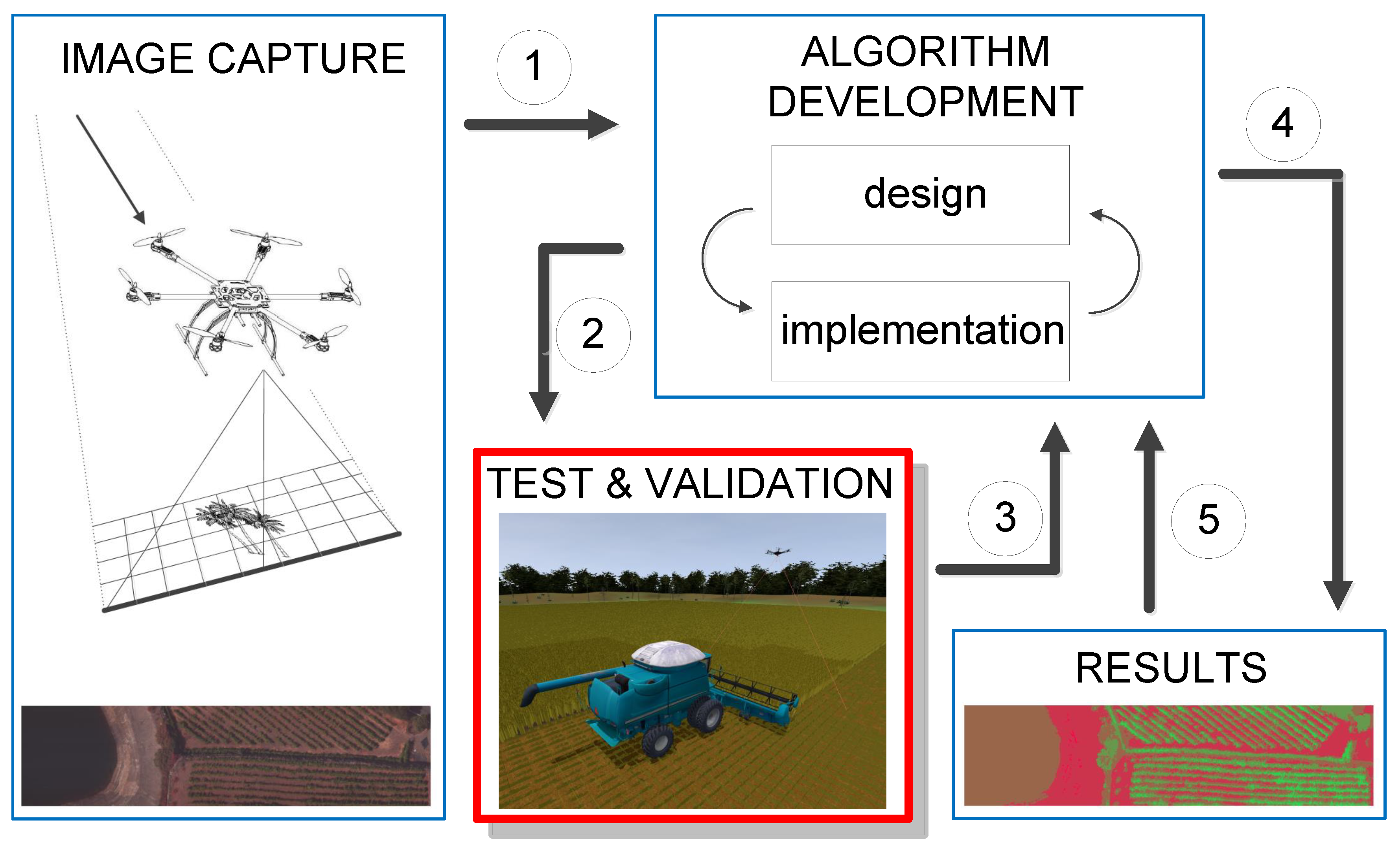
The contribution of this work consists in bringing in a novel intermediate phase for testing and validating the behaviour of hyperspectral image processing algorithms for real-time systems, based on a simulation environment that provides a faithful virtual representation of the real world. Figure 1 shows all the involved stages, including the new one proposed in this work, highlighted in red, which significantly shortens the gap between the offline image processing algorithm implementation and its use in a real scenario. In particular, the work uncovered in this paper is based on using a pushbroom hyperspectral camera, that presently constitutes one of the most widely chosen sensors to be mounted on a UAV [8,9] due to its trade off between spatial and spectral resolution. The integration of this type of camera into a UAV is nonetheless a rather complex task since the captured frames are individual lines that share no overlapping, and hence, much more effort has to be put into the acquisition and processing stages, in order to generate a 2D image.

The virtual environment developed in this work offers the possibility of simulating and stimulating the sensor, virtually creating hyperspectral images as they are captured by the targeted hyperspectral sensor and applying the processing algorithms to them in order to obtain the results straight away. In this way, before performing a real testing with the whole system, simulations can be run several times making modifications in the code and/or in the input parameters. This shortens the testing phase and reduces the required overall manpower required, what in the end translates into considerable cost savings in the whole system implementation.

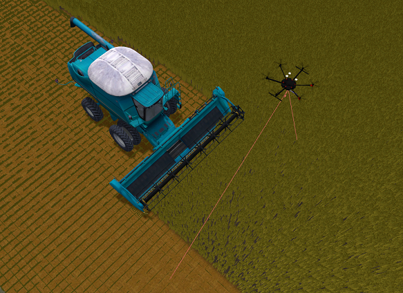
The research presented in this paper has been demonstrated within the frame of a use case of a European H2020 ECSEL project named ENABLE-S3 (European Initiative to Enable Validation for Highly Automated Safe and Secure Systems) [10]. The goal for this particular scenario called “Farming Use Case” [11], is the automated driving of a harvester in an agricultural field performing the cropping, watering or pesticide spraying tasks. Initially, a drone equipped with a hyperspectral camera inspects the terrain in order to generate a set of maps with different vegetation indices which give the information related to the status of the crop. This information, together with the specific coordinates, is then sent to the harvester, which initiates its autonomous driving to the region of interest and starts its labour. Additionally, in order to minimize the risk of fatal accidents due to agricultural mowing operations and/or collisions with big obstacles (animals or rocks), the scheme shown in Figure 2 has been considered, in which the drone flies at a certain height above ground, and some meters ahead of the harvester (security distance) scanning the field for the possible appearance of static or dynamic objects. Hence, due to the criticality of the decisions that have to be made in real-time within this use case, it is recommendable to count with the proposed environment in order to exhaustively evaluate the behaviour of the whole system in a realistic way before operating in the field.

At this point, it is important to highlight that in order to cope with the requirements of the mentioned use case, we have utilized the preexisting agriculture graphical simulation environment (AgSim) which is able to virtually recreate the different scenarios considered within the ENABLE-S3 farming use case, introducing different machinery such as a harvester, a tractor, and a drone onto a farming field. In this work, just a part of the proposed simulation environment is presented, i.e., the one that focuses on the drone and its sensor (the on-board hyperspectral camera), all together being considered as the device under test. More precisely, the system that has been simulated is the one presented in [12], based on a Matrice 600 drone [13] and a Specim FX10 hyperspectral camera [14]. As it will be further detailed, the proposed environment is able to simultaneously test the drone control routines together with the capturing and processing of the hyperspectral images. This software in the loop testing setup permits the validation and verification of different hyperspectral image processing algorithms such as image generation, vegetation indices map creation and target detection. Finally, it is worth to mention that the proposed tool has been conceived in a modular way, hence different real time processing algorithms can be tested or different hyperspectral sensor characteristics can be used, just by replacing the corresponding module, which represents yet another contribution of this work.

The rest of this manuscript is organized as follows. Section 2 introduces the AgSim environment as an actor that allows to virtually recreate a realistic farming scenario in which we can test the benefits of the proposed simulation environment for the validation and verification of real-time hyperspectral image processing algorithms on-board a UAV. Section 3 presents the proposed hyperspectral simulation environment and its main elements. Section 4 introduces the creation of two types of hyperspectral scenarios: target detection scenarios, presented in Section 4.1, and map scenarios based on real bitmaps, presented in Section 4.2. Section 5 displays the results using the scenarios presented earlier. In Section 5.1, target detection scenarios are used to test an anomaly detection algorithm, while in Section 5.2, a virtual mission flight results are laid out. Finally, Section 6 discloses the obtained conclusions and outlines further research lines.

2. The Agriculture Graphical Simulation Environment: AgSim

The agriculture graphical simulation environment, AgSim, has been utilized in this work in order to recreate a virtual farming domain in which the proposed simulation environment is validated. The simulated scenario consists of a farming field together with a harvester, a tractor with trailer, and the already mentioned drone. AgSim is comprised of two main parts: the simulation engine and the 3D visual system. Machine models, i.e., harvester, tractor and drone models, are built on top of the simulation engine which interfaces to external control systems, either simulated, in case the testing setup is a software in the loop (SiL), or a real controller, in case the testing setup is a hardware in the loop (HiL). A script-based test command interface is used to load test cases and to set proper initial state for the machine simulation variables. Based on the control system behaviour and test script control of the real time simulation, results are produced for the test case evaluation.

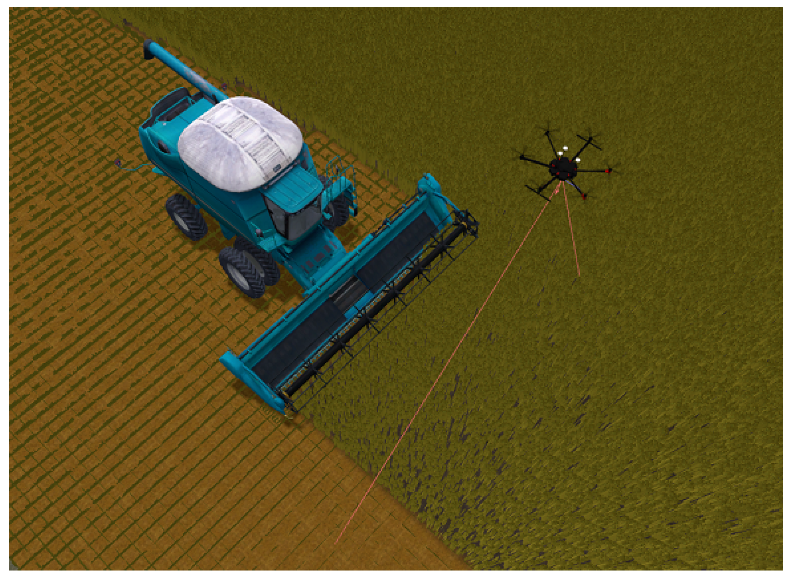
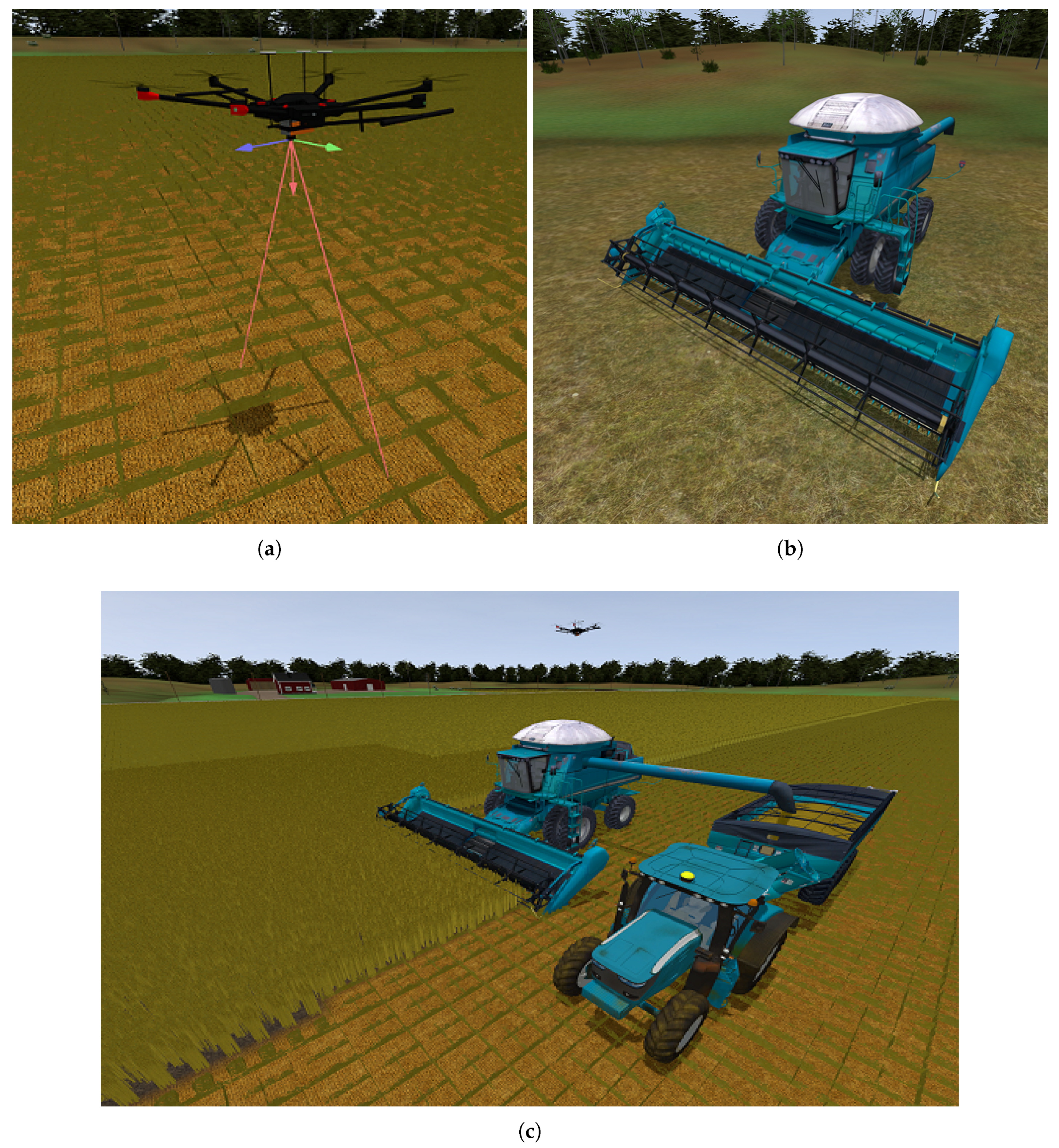
Figure 3 shows the main equipment simulated in the AgSim environment. The drone with the hyperspectral camera, its axis and the vision scope can be seen in Figure 3a. In Figure 3b, the combine-harvester is presented. Figure 3c displays a parallel driving representation involving all the autonomous vehicles available in the AgSim environment, namely, the combine-harvester, the tractor and the drone.

The 3D visual system helps the final user to see the simulated events, allowing to check that the simulation runs as expected and fulfills the machine operation requirements under test. The initial state of a testing scenario may contain a description of different situations and events. These are, for instance, stationary or moving objects, obstacles not known by the control systems, or animals running on the field, just to name some. The simulated models of the machines have interfaces for external control algorithms running in Python. The simulation environment supports the hardware in the loop testing setup through I/O boards or adapters for serial communication such as CAN or Ethernet connected to real embedded control modules. As an example, also within the project ENABLE-S3, the partner TTControl has integrated one of their electronic control units (ECU), the model HY-TTC 580, into the AgSim using CAN signals.

3. Proposed Hyperspectral Simulation Environment

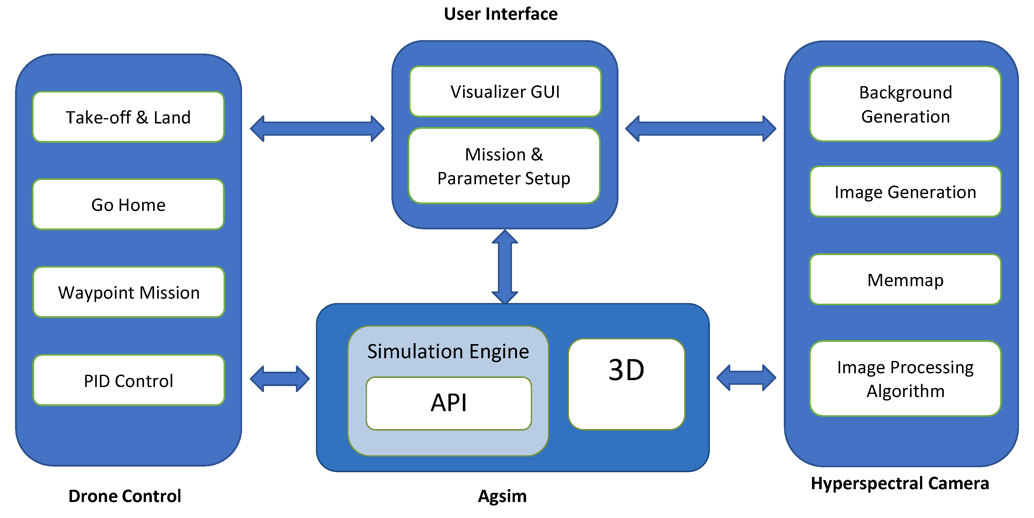
The main purpose of creating the proposed hyperspectral simulation environment is to be able to validate and verify real-time image processing algorithms in combination with flight control functions within realistic scenarios. Figure 4 displays the diagram of the implemented system in terms of functional modules. As it is seen, it has been designed and programmed in a modular way, easing the replacement of modules if another hyperspectral sensor and/or image processing algorithm is to be tested. Another important aspect that supports the mentioned modularity is the parameterization of the whole environment, making use of configuration files that are loaded when the system is started.

The whole system is comprised of four main modules: the user interface module, the hyperspectral camera module, the drone control module, and finally, the AgSim environment already introduced. It is important to highlight that these four modules run in separate threads completely decoupled one from another.

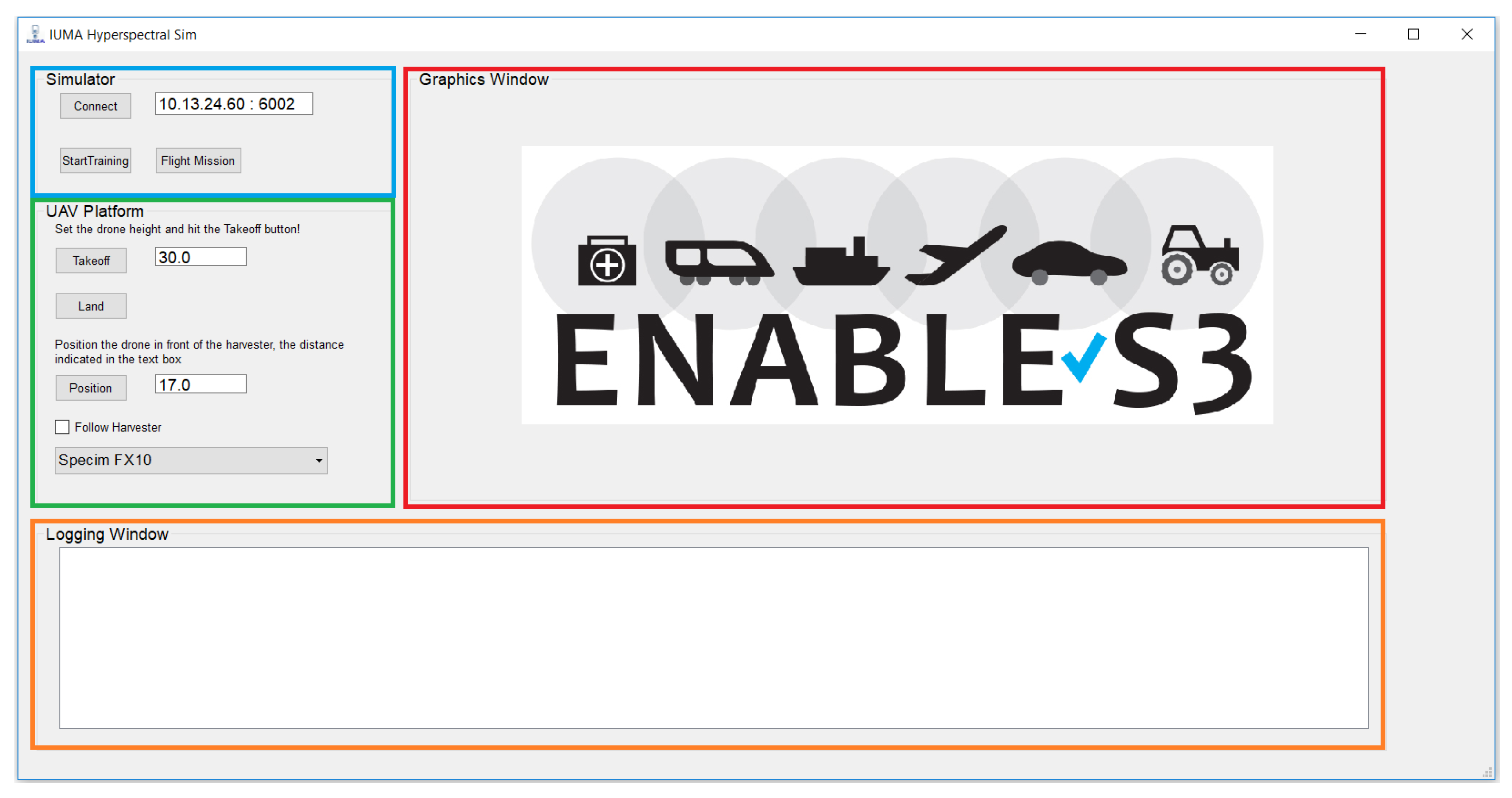
The user interface in Figure 4 is made of a visualizer where images are displayed, the mission is selected and its parameters are setup by the user. Figure 5 displays the layout of the main user interface window, where its different sections are shown. The first section, highlighted in blue, is meant for the simulation environment’s main functions, such as establishing a connection at a given IP address and port number, starting a specific training loaded from memory and opening the flight mission window to setup a custom mission, as it will be later detailed. Highlighted in green is the section related to the UAV platform, where it can be issued a takeoff command at a predefined height above ground, land the drone, position it in front of the harvester at a given distance and start the follow function routine (where the drone stays ahead of the harvester a selected distance), and inspecting the field. At the bottom of this section, a drop-down menu is available where the targeted hyperspectral sensor is selected. The section on the right, in red, is the graphics window where synthetic hyperspectral images are displayed in real time, as they are being generated while a mission is running. If a target detection mission is being executed, the window is split into two, in order to show the false RGB composition of the synthetic image on one display, and on the other one, the real time processing result obtained with the applied anomaly detection algorithm. Finally, the bottom panel, highlighted in orange, displays relevant information for the user in a logging window.

The drone control module in Figure 4 creates an instance of the AgSim drone and implements functions such as take-off and land, return home, perform a flight mission according to the defined waypoints, and a PID control that allows the drone to follow another vehicle, i.e, the combine-harvester. These implemented functions are based on application programming interface (API) drone functions that will be discussed later in the section.

As it was mentioned before, the hyperspectral camera module runs in a different process than the other main three modules, hence a data sharing policy has to be implemented for the other processes to access the captured images, and a synchronization mechanism between the capturing process and the flight in order to capture images at the desired sectors. The block that facilitates such implementation is the $memmap$, also displayed in Figure 4. It mainly consists of a memory block that buffers a predefined number of captured frames into the system RAM memory as well as other signals, such as the camera trigger and the image data type, among others. The memory mapped by the $memmap$ block is accessible by all other processes running in parallel within the application software, permitting, for instance, that the image visualization, processing or storing in memory of data take place simultaneously. This block is implemented using the homonymous library from Python which essentially works as a shared memory that is initialized with a unique id and the required memory size.

Regarding AgSim, as it was previously introduced, it includes an API that can be used for externally controlling the machinery through available commands and read out sensor signals. This API connects to the environment software via a transmission control protocol/internet protocol (TCP-IP) tunnel and it is programmed using Python language. It is mainly used to support external models and external sensor simulations, enabling the possibility of defining and running test cases which interact with the environment.

Table 1. Agriculture graphical simulation environment (AgSim) application programming interface (API) drone functions.

Function	Description
CaddRotation	Set rotation angle to turn the drone on Z-axis.
getPixelData	Get hyperspectral pushbroom camera pixel data.
getPose	Get position and orientation of a drone.
isLandingGearDown	Check if the landing gear is down.
setConnection	Set Creanex simulator remote services instance for the module.
setDroneEngineRunningState	Set drone engine to on or off.
setLandingGearState	Set drone landing gear state.
setVelocity	Set velocity vector for the drone.

presents the main API functions to control the drone. First, a drone instance has to be created by setting a proper connection, using the right IP address and port, and afterwards, the control commands and signals are ready to be called.

As mentioned before, AgSim offers the capability of reading out pixel label information that can be transformed into sensor data. The information provided per line of pixels by the tool depends on how many materials from a predefined list of materials are present in the line, which materials are they, and in which proportions are they mixed in each pixel of the sensed line. With this information and the stored hyperspectral signature of each material, the tool is able to generate the synthetic hyperspectral images that emulate the targeted scenario. 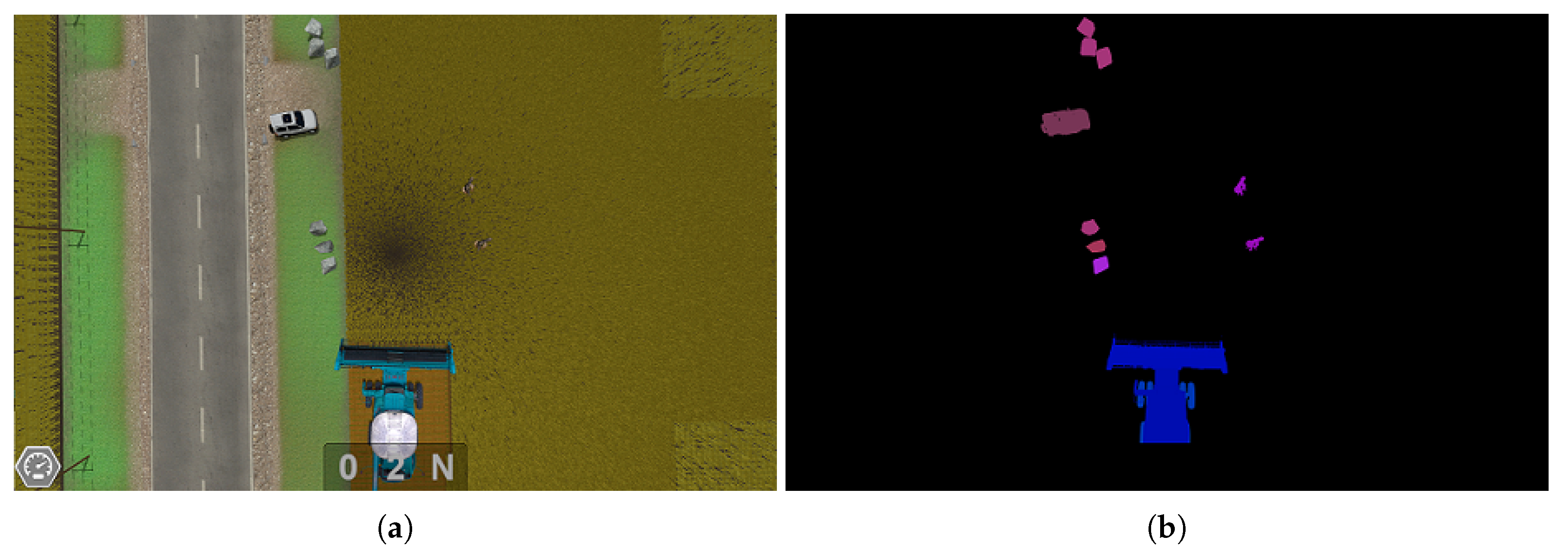Figure 6 shows how the material label assignment works. In Figure 6a, the scenario from the drone perspective is shown, where it can be seen that some objects have been placed in the environment, such as a car, some rocks and two mooses located in the center of the image. In Figure 6b just the material label image is shown, highlighting in different colors each material group. Last but not least, it is worth to mention that the same procedure has been applied to other sensors mounted on the harvester, such as radar sensors [15].

4. Creation of Hyperspectral Scenarios

The proposed simulation environment works with two hyperspectral scenarios aided by the generation of synthetic images in two different fashions. On one hand, the scenarios created for target detection to test hyperspectral anomaly detection algorithms. On the other hand, the generation of hyperspectral maps based on a real grayscale bitmap overlayed on top of the virtual scenario, that allow testing geometric correction algorithms.

4.1. Target Detection Scenarios

The creation of synthetic target detection scenarios is based on the process described in [16], with a set of adjustments that will be discussed throughout this section, due to the fact the process was not conceived for real time applications.This synthetic image generation process can be split into two parts: the background generation and the insertion of anomalies.

The background generation follows the linear unmixing principle [17]. This is based on the idea that each captured pixel in a hyperspectral image, $M=[r_1,r_2,\dots ,r_{N_p}]$, which is composed by $N_p$ pixels with $N_b$ spectral bands each, can be represented as a linear combination of a set of p spectrally pure constituent spectra or endmembers, e, weighted by an abundance factor, a, that establishes the proportion of each endmember in the pixel under inspection. This is shown in Equation (1), where $e_j$ represents the j-th endmember signature, p is the number of endmembers in the image and $a_{i,j}$ is the abundance of endmember $e_j$ in the pixel $r_i$. The noise present in the pixel $r_i$ is contained in the vector $n_i$.

$$r_i={\displaystyle \sum _{j=1}^p}{e}_j·a_{i,j}+n_i$$

(1)

For the synthetic image generation, the endmembers are the background signatures stored in memory which are combined based on the generated abundances. There are two main methods to obtain the abundances as described in [16], Legendre and Gaussian fields, and within the latter, four extra options appear, depending on the selected type: Spheric, Exponential, Rational and Mattern. In this work, Spheric Gaussian fields have been extensively used due to the pattern resemblance to a cropping field and its higher adaptability to a real time calculation thanks to the slightly simpler operations involved. The steps followed are described below:

(a)

The number of endmembers used to create the background is set to four. Endmembers are selected from real images taken over a vineyard and from a database, as it will be described later.

(b)

The simulated abundance image for each endmember is computed as a Gaussian random field following the procedure proposed in [18]. Since this process is computationally intensive, it has been split into the calculation of a matrix called $lambda$, performed offline using different $theta$ values which define the size of the gaussian spheres. The rest of the process, which contains the random part, is executed in real time. The $lambda$ matrices are stored in memory and the one selected by the user loaded during run-time.

(c)

The abundances of each pixel are normalized. The greatest abundance coefficient value is preserved, normalizing the remaining coefficients to ensure that the sum of the abundance coefficients gives one as a result.

Generating the abundances for the background of an image of size $1024\times 100$ pixels takes about two seconds, clearly beyond the simulator minimum step time of 20 ms, which has been established after running tests on machines with different characteristics with the goal of ensuring that no frame is dropped. For this reason, the background generation is performed in a different block that is launched in a separate thread that runs in parallel. Every time it is executed, a buffer of b lines is generated, so when the main process needs a new line to create a new hyperspectral synthetic frame, a line from the buffer is withdrawn. When the number of lines in the buffer goes below a predefined threshold, the background generation function is invoked again to fill it up.

The insertion of anomalies is the last step in the synthetic generation process. Spectral signatures of the labels available in AgSim are stored in memory and every time a specific label is present in the field, its spectra is inserted in the image at the specific pixel location. In order to make it more realistic, the final pixel array is a combination of the background and the anomaly spectra equally proportioned.

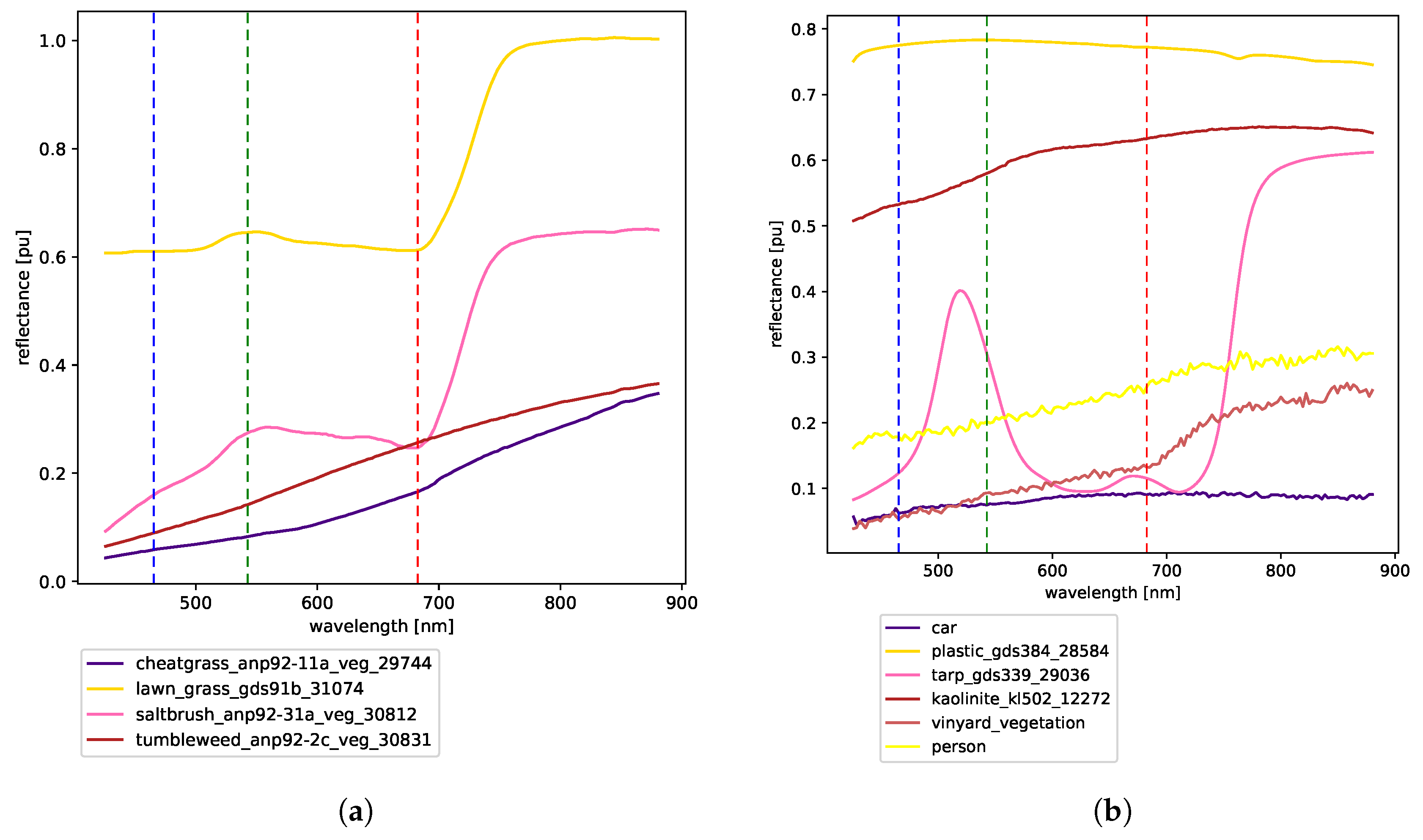
The spectra to be used in the synthetic generation of hyperspectral images must be carefully selected. In this particular case, both real spectra captured with the Specim FX10 on-board a UAV [12] and from a spectral library collected from the United States Geological Survey (USGS) [19] have been used. Since a specific hyperspectral sensor is being tested, signatures not captured with this camera shall be interpolated to its wavelengths. The FX10 has 224 bands spanned in the range of 400 nm to 1000 nm. However, due to the low signal-to-noise ratio (SNR) of the first and last spectral bands, bands 1-11 and 181-224 have been removed, so that only 169 bands are retained. Figure 7 displays the spectra used to obtain the background, represented on chart Figure 7a, and some of the spectra selected for the anomalies, represented on chart Figure 7b. For instance, the spectra named “car”, “person” and “vinyard_vegetation” were obtained on a real flight at 45 m of height above the ground, during a flight campaign presented in [12].

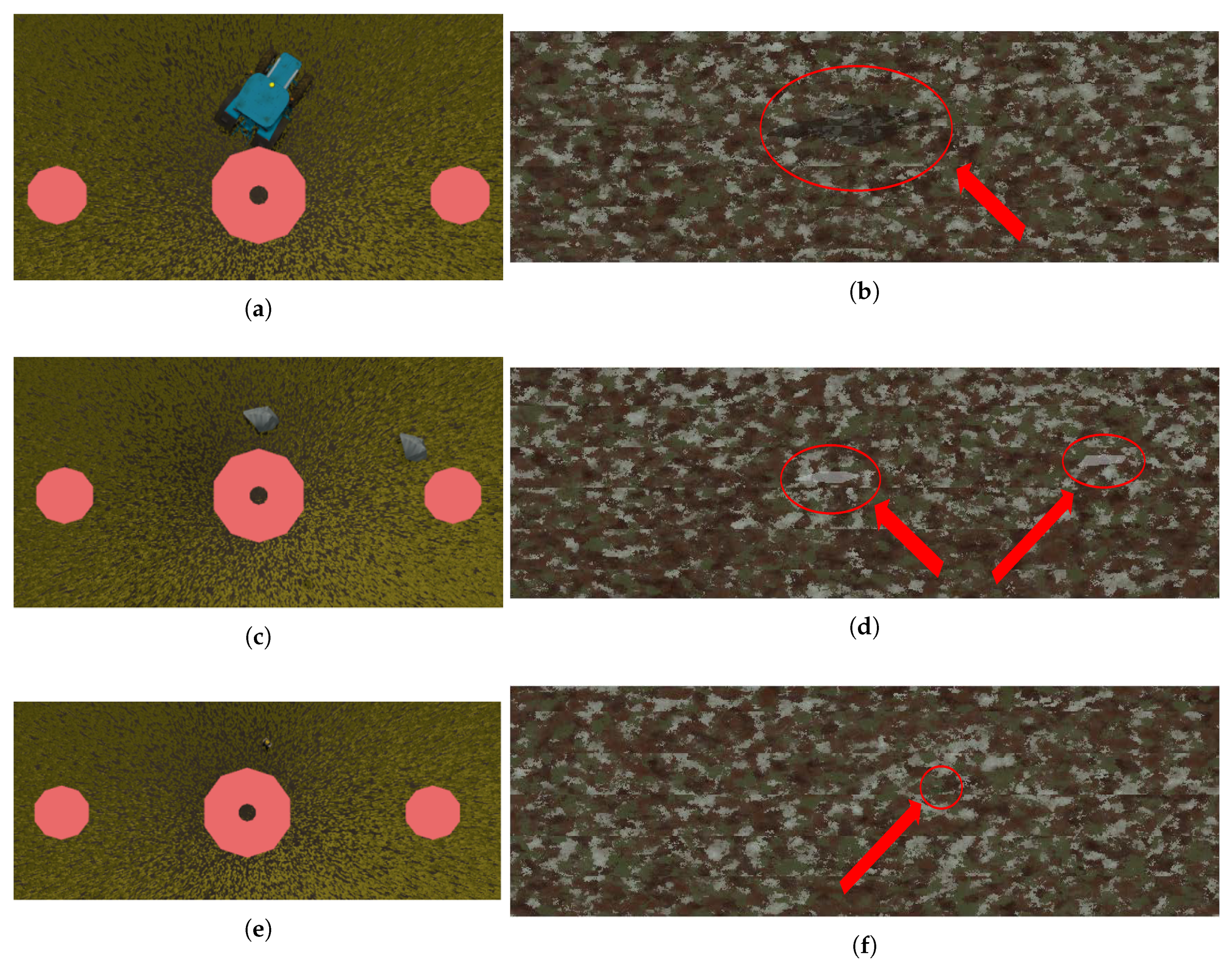
Figure 8 shows examples of the synthetic image generation process in which the virtual tool inserts different objects. For the representation of the synthetic images, a false RGB composition has been created. In Figure 8a, the drone view of the field is represented with a tractor incorporated to the scene. The synthetic image of that view from the drone is represented in Figure 8b. Figure 8c shows two rocks located on the virtual scene and the synthetic image of that view is represented on Figure 8d. Finally, in Figure 8e, a human being has been placed on the scene and its synthetic image is shown in Figure 8f. For clarity, the anomalies placed on the synthetic image has been circled in red and pointed with an arrow.

4.2. Hyperspectral Map Scenarios Based on Real Bitmaps

The creation of hyperspectral maps from a set of images taken over a field faces several challenges in the real world, in the sense that it is paramount to have a steady drone flight to achieve a proper image capture. In fact, if the goal is to obtain a high quality map, an image geometric correction process is unavoidable.

For this purpose, the proposed tool acquires the required additional data to perform such correction, which mainly consists of the drone position and orientation at the time every capture takes place. As it was previously mentioned, the image capturing process and the drone flight control are completely decoupled, therefore, both the frame timestamp and the position and orientation timestamp are stored separately in different files to later perform an interpolation.

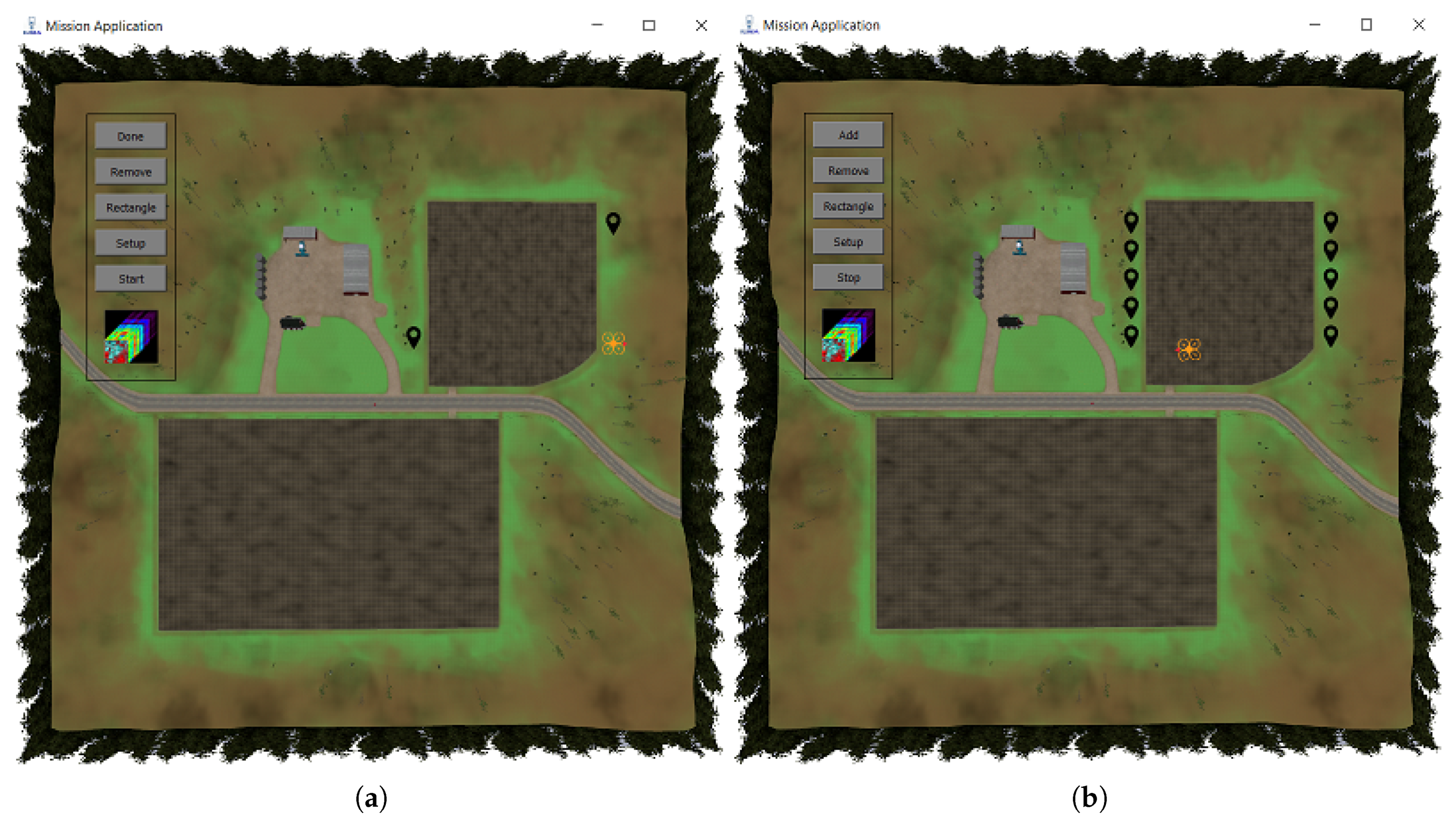
In order to obtain the hyperspectral map, the first step is to create a flight mission. Figure 9 shows the user interface created for the purpose of selecting a region of interest to be scouted and laying out the waypoints. The steps followed for the waypoints layout are defined below:

• First, the user selects the diagonally opposed rectangle corners providing the result shown in Figure 9a. After that, the other two corners are internally calculated and added to the interface.
• Second, the shortest distance of the created rectangle is selected to lay down additional waypoints in between those corners. In this way, each individual flight swath has a bigger length and therefore, the flying time is reduced. It has to be mentioned that distances in AgSim are defined in meters, being the reference coordinates located at the center position of the virtual environment.
• Third, when the user clicks the setup button, a new window appears requesting the following parameters:
  • relative height, h, from the ground, in $meters$
  • frames per second, in $FPS$
  • overlap of captured swathes, in %, in order to facilitate a mosaicking process.
• Fourth, based on the inputs provided by the user in step 3, the image width in meters is obtained by multiplying the resolution by the spatial sampling of the camera and corrected with the input overlap.
• Finally, the number of waypoints to be added in between the corner waypoints is calculated and added to the user interface, as indicated in Figure 9b.

The calculation of the number of waypoints is performed using the formulas defined below:

$$widt{h}^{\prime }=width\ast \left(1-\frac{overlap}{100}\right)$$

(2)

$$N_{\mathrm{waypoints}}=\left({\displaystyle \frac{side\_distance}{widt{h}^{\prime }}}-1\right),$$

(3)

where $side\_distance$ is the distance in meters of the shortest rectangle side. As this calculation does not always provide an integer number, the result is rounded up to the next integer value, giving as a result a larger overlap between images than what it was previously defined.

Based on the given inputs defined before, the drone flight speed shall be obtained in order to capture the whole scene. The formulas defined below are applied for the speed calculation:

$$\mathrm{resolution}={\displaystyle \frac{spatial\_sampling}{2\ast h\ast tan{\displaystyle \frac{\alpha }{2}}}}$$

(4)

$$\mathrm{speed}=\mathrm{resolution}\times FPS$$

(5)

Equation (4) defines the resolution based on the camera and flight parameters, such as the camera $spatial\_sampling$, field of view, $\alpha$, and the flight height, h.

As previously indicated, the tool lets the user define a bitmap pattern in order to simulate a real scenario. The reason why bitmaps are used, instead of other type of images, is because they can be ranged from 0 to 1, what enables the creation of hyperspectral maps. For instance, if the pattern is an already obtained result of a normalized difference vegetation index (NDVI) [20], ranged between 0 and 1 as well, pixels of the pattern can be replaced by spectra from a database that has the same NDVI value.

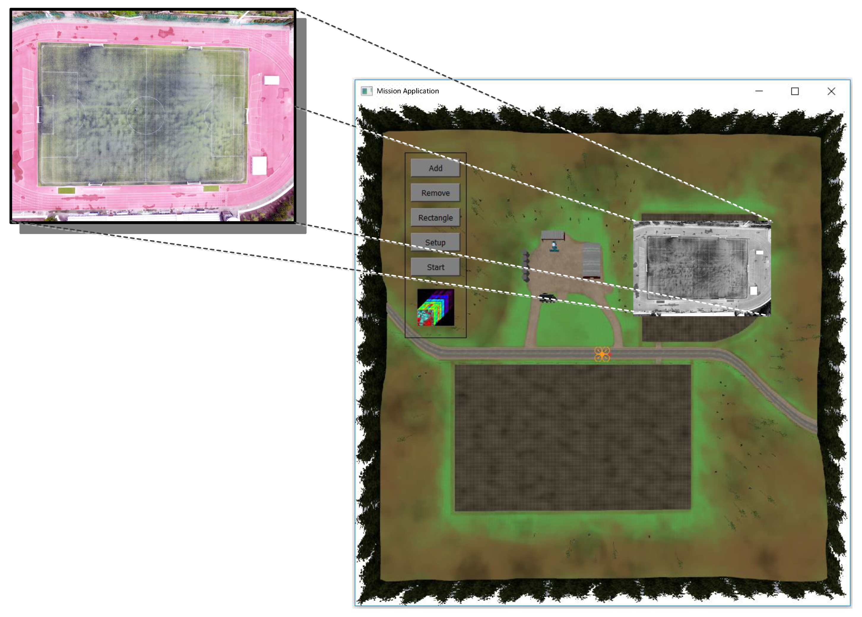
In our case an image taken from the football field located at the University of Las Palmas de Gran Canaria campus has been used, due to the fact that it presents straight lines which are an excellent visual inspection tool to check distortions in the captured swathes as well as the created mosaic. GPS coordinates of the football field are 28°04${}^{\prime }$17.9${}^{″}$N 15°27${}^{\prime }$25.9${}^{″}$W. Figure 10 shows the pattern image on the left, taken with a Phantom 4 UAV at a height of 80 m and on the right hand side, the image has been placed in the upper right corner, on top of the cropping field.

The procedure to import the image to AgSim is done manually, even before the software is started, consisting of two main steps. First, the image has to be converted to grayscale values. Secondly, in the AgSim configuration files, the simulation scenario corner positions where the pattern is to be placed are defined in meters. For this purpose, it is important to know the width and height of the imported image in order to avoid having any distortions in the final result.

Obtaining the width and height of the image in meters requires knowing the field of view (FOV) and the image resolution. In this case, the Phantom 4 has a camera FOV with 94° in diagonal, and a resolution of $3000\times 4000$ pixels. Based on these values, the image taken at 80 m of height has a width of 137 m and a length of 103 m.

5. Results

The scenario creation presented in the previous section can potentially be used to test the performance of two different types of algorithms: anomaly detection algorithms and geometric correction algorithms.

In this section, the tests performed with specific image processing algorithms for these two applications are presented.

5.1. Anomaly Detection Algorithms

The scientific community has invested a huge effort in creating new algorithms to tackle the anomaly detection problem. The most well known is the Reed–Xiaoli (RX) algorithm [21], which is one of the first developments in this field, and nowadays, it is considered as a benchmark to which other methods are compared. Several variations of the RX detection technique have been proposed in order to improve its performance. Subspace RX (SSRX) [22] and RX after orthogonal subspace projection (OSPRX) [23] are global anomaly detectors that apply principal component analysis (PCA) or singular value decomposition (SVD) to the datacube.

In the recent years, new approaches to the problem have emerged in order to cope, for instance, with inadequate Gaussian-distributed representations for non-homogeneous backgrounds [24], the presence of noise in the images, by using a combined similarity criterion anomaly detector (CSCAD) method [25], as well as the removal of outliers by using a collaborative representation detector (CRD) [26,27].

However, the above algorithms are not suitable for those applications that demand a real-time response, since they require the sensing of the whole hyperspectral image before starting with the process of finding the anomalies in the captured scene. The hyperspectral sensor considered in this work is a pushbroom type scanner, meaning that the image is captured in a line-by-line fashion. For applications under strict real-time constraints in which the captured images must be processed in a short period of time, it is more efficient if the anomalies are uncovered as soon as the hyperspectral data are sensed. For this purpose, there have been recent solutions proposed to cope with this situation [28,29,30].

In the next part, the results of the line by line anomaly detection (LbL-AD) implementation [29] are presented as an example of how extensively the algorithm can be tested and what type of results the proposed tool is able to provide.

The LbL-AD implementation has a set of fixed parameters that have to be set before its execution. In this manuscript, the results of the algorithm varying the parameter d, which is the number of eigenvalues and eigenvectors to be calculated when applying the transformation to the new subspace, are displayed.

Table 2. Results from two simulation runs, changing the algorithms parameter d.

(a) Simulation run of 51.5 s, 1030 frames captured and d set to 5.					(b) Simulation run of 44.85 s, 897 frames captured and d set to 4.
		Ground truth		Positive rate			Ground truth		Positive rate
		✚	▬				✚	▬
Results	✚	171442	56	0.9967	Results	✚	1587	15	0.9906
	▬	1017	1036503	0.999		▬	12321	904605	0.9866

shows the results of two simulation runs changing the mentioned parameter (it has been set to 5 in the Table displayed on the left and to 4 in Table on the right ). The displayed values on the tables are the true positives (TP) on the top left hand side and the false negatives (FN) on the bottom left hand side. On the right hand side, from top to bottom, false positives (FP) and true negatives (TN) are respectively displayed.

In order to obtain normalized metrics that let us compare the results between different simulation runs, a true positive rate (TPR) and a false positive rate (FPR) have been defined as:

$$TPR={\displaystyle \frac{TP}{TP+FP}}$$

(6)

$$FPR={\displaystyle \frac{FP}{TP+FP}}.$$

(7)

The TPR is the probability that the anomaly is present when the test is positive and the FPR is the probability that the anomaly is not present when the test is negative. As it is seen in Table 2, when the number of eigenvalues is decreased the number of false negatives substantially increases, mainly because the new calculated subspace does not contain enough information to detect all the anomaly signatures. This translates into a lower FPR, which for the specific application of the ENABLE-S3 project is quite critical since one of the goals is the avoidance of fatal accidents. Therefore, for such application, it is desirable to achieve a FPR as close to 1 as possible.

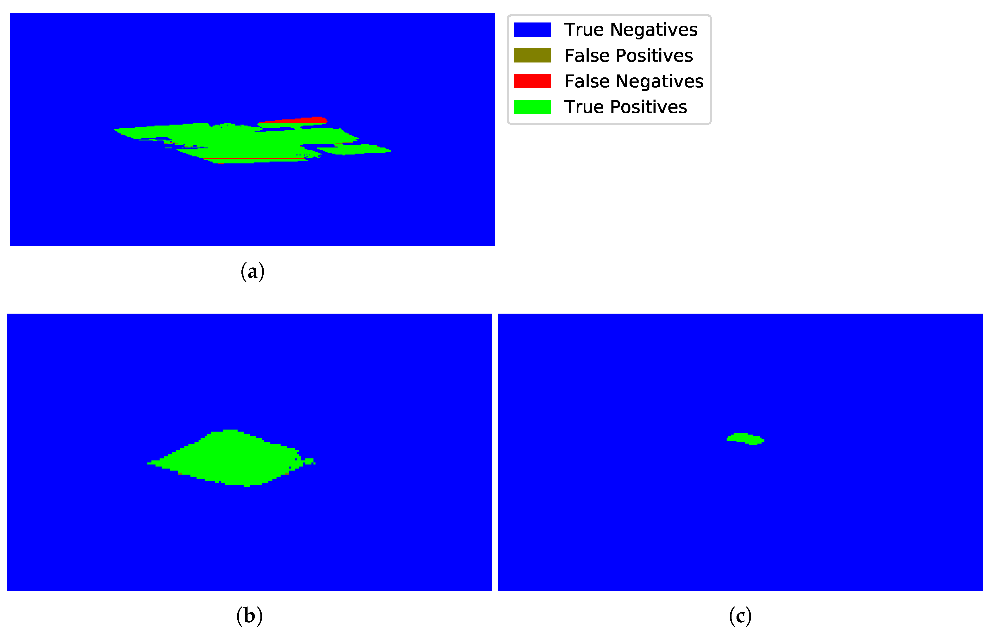
Figure 11 visually presents the results previously shown in Table 2, with parameter d set to 5. It has to be highlighted that in order to produce these results and the ones shown in Table 2, the output of the algorithm has been binarized using a threshold. In Figure 11a the detection of a tractor is depicted, showing some false negatives, probably due to a non-optimal threshold set. Figure 11b,c show the results of a rock detection and person detection, respectively. In both cases, just a few false positives are present in the result.

5.2. Mosaic Creation Algorithms

UAV platforms equipped with vision sensors are normally used to scan large fields that require the platform to split the area in several sectors which are assembled together in an ulterior post-processing stage. In case of dealing with pushbroom sensors the situation becomes complex since the captured frames/lines within each sector share no overlapping so they are subjected to miss-alignments due to adverse weather conditions, mainly wind, during the flight that need to be corrected.

The scientific community has put a lot of efforts in this post-processing phase, correcting remotely sensed images both, geometrically and radiometrically, either by having a very precise positioning system in order to know the camera orientation and position for every frame [31] or by having incorporated an RGB snapshot sensor [32] that through image processing is able to make a 3D reconstruction and obtain the hyperspectral camera features in each captured frame.

The geometric correction process is performed in two steps. First, determining the position and orientation of the platform at the time every capture takes place, based on the information provided by other sensors available. Secondly, using the aforementioned data to project the image onto a plane and perform the necessary interpolations when required.

The first step, the position and orientation of the platform can be easily obtained in the simulation environment with a high degree of accuracy. Then the algorithms corresponding to the second step are run in order to obtain a final result.

The potential of the presented system is that, in order to test the geometric correction algorithms, the position and orientation data can be altered, for instance, by adding some distortions or by obtaining samples in a lower rate than the image capturing frame rate, testing the robustness of the mentioned algorithms.

The results of a mission performed in the simulation environment are presented next.

Table 3. Waypoint mission setup.

Inputs	Height [m]	50	Outputs	Speed [m/s]	0.84
	Frame rate [FPS]	25		Resolution [m]	0.0336
	Overlap [%]	40		Scanned Area [m${}^2$]	31,519.88
	Area [m${}^2$]	14,773.47		Number Waypoints [–]	10

depicts the mission parameters, with the inputs defined by the user on the left hand side, and on the right hand side the values calculated using Equations (2)–(5). After having calculated all the required parameters, the application proceeds to layout the mission waypoints, which matches the setup already presented in Figure 9b.

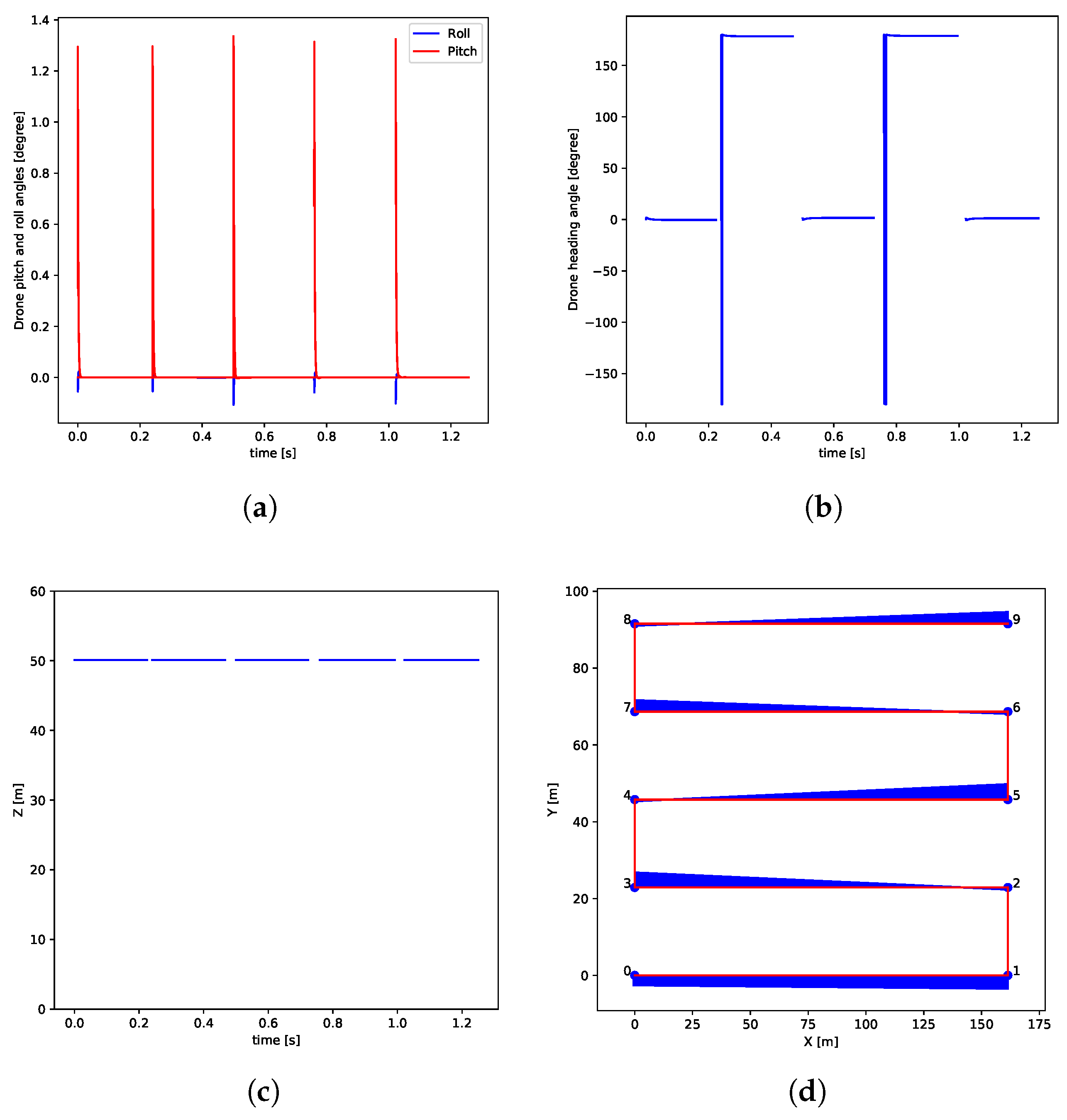
As mentioned before, during the mission, the system records important data that serves both to analyze the flight, as well as input to the geometric correction algorithms. In Figure 12, the UAV platform signals recorded during the flight are shown. Roll and pitch angles are depicted in Figure 12a. Discontinuities in the chart come from the fact that data are just recorded in the long sectors when images are also being captured, therefore, only five different sectors are displayed in the Figure 12. Drone heading angle is presented in a separate graph (Figure 12b) due to the scale difference in the Y-axis compared to the other two orientation signals. The same five sectors are shown in Figure 12c, where altitude above ground values are plotted. Finally, the real trajectory versus the ideal one is presented in Figure 12d, in blue and red, respectively.

Analyzing the data presented in Figure 12 it is confirmed that this is a very stable flight compared to an actual one performed by a real platform based on a UAV with a hyperspectral camera as payload. Altitude above ground stays almost constant throughout the whole flight, the roll and pitch angles show a slight peak at the beginning of the sector but then remain constant, while the trajectory is the only one that looks more alike a real situation deviating considerably especially in sectors 2 and 4. From these charts it can be inferred that the intra-sector miss-alignments are going to be negligible, and therefore, the captured lines are fitting well one after the other without having to apply a geometric correction algorithm, which is unfortunately not the case in a real scenario. Nonetheless, the aim of this work is to present the methodology for testing algorithms using virtual environments and we certainly acknowledge that the proposed environment should be further improved, trying to bring it closer to a real situation by, for instance, incorporating weather phenomena, such as wind and dust, among others.

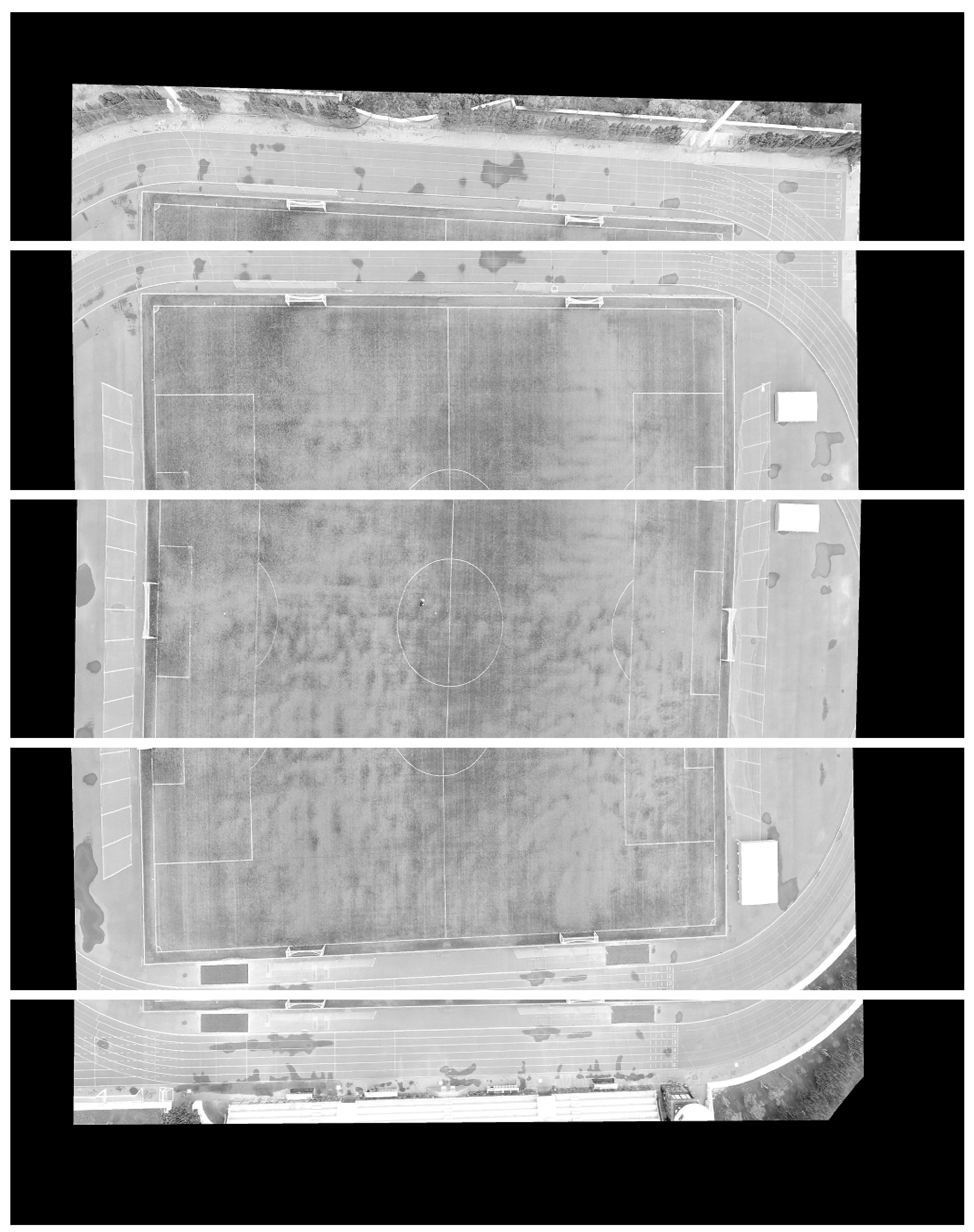
In Figure 13, the captured swathes per each sector are displayed. There were 10 waypoints layout in the map, thus, five swathes were captured. Here we can check that the assumption made before about the lack of intra-sector distortions was correct. There is however a slight rotation distortion between sectors that was also appreciated in Figure 12d. Anyhow, this effect is not corrected in the flight control code, since it is preferable to have a straight line rather than rotations and changes of trajectory in the middle of the sector in order to facilitate the post-processing algorithm’s task.

6. Conclusions

The validation and verification (V&V) process during the development cycle of any commercial product represents a high percentage of its success as they define the product functionality and its reliability. Autonomous systems require a tough battery of testing in different scenarios in order to ensure low risk affecting humans and/or costly equipment. However, there is a balance between financial aspects and time to market when conducting these tests in the real world, and repeating exactly the same testing conditions, time after time, is not an easy task and in many times impossible to reproduce. This is especially true for the particular case of UAVs, in which climate (mainly wind and rain) is unpredictable and affect the performance of these flying platforms. A new level of difficulty is introduced depending on the target application. For example, using UAVs and spectral sensors in precision farming means dealing in some cases with temporary croplands which in the worst case feature a one-year growing cycle. In order to deal with all of these variables, in this work a hyperspectral simulation environment has been presented to analyze the virtual behavior of a UAV equipped with a pushbroom hyperspectral camera used for harvesting applications. As result, this tool alleviates the process of testing different phases involved in the automation of future farming such as image generation, health status inspection and target detection. As a future line, the perturbations from wind and other climate phenomena should be brought into the physical model of the AgSim environment to be able to have an even closer representation of real scenarios with additional distortions, testing the algorithms in tougher conditions.