Article

Remotely Sensed Water Limitation in Vegetation: Insights from an Experiment with Unmanned Aerial Vehicles (UAVs)

1
Department of Environmental Sciences, Policy and Management, University of California, Berkeley, CA 94720, USA
2
Department of Integrative Biology, University of California, Berkeley, CA 94720, USA
3
University of California Division of Agriculture and Natural Resources, Davis, CA 95618, USA
*
Author to whom correspondence should be addressed.
Remote Sens. 2019, 11(16), 1853; https://doi.org/10.3390/rs11161853
Submission received: 3 July 2019 / Revised: 30 July 2019 / Accepted: 6 August 2019 / Published: 9 August 2019
(This article belongs to the Section Remote Sensing in Agriculture and Vegetation)

Abstract

:
Unmanned aerial vehicles (UAVs) equipped with multispectral sensors present an opportunity to monitor vegetation with on-demand high spatial and temporal resolution. In this study we use multispectral imagery from quadcopter UAVs to monitor the progression of a water manipulation experiment on a common shrub, Baccharis pilularis (coyote brush) at the Blue Oak Ranch Reserve (BORR) ~20 km east of San Jose, California. We recorded multispectral imagery at several altitudes with nearly hourly intervals to explore the relationship between two common spectral indices, NDVI (normalized difference vegetation index) and NDRE (normalized difference red edge index), leaf water content and water potential as physiological metrics of plant water status, across a gradient of water deficit. An examination of the spatial and temporal thresholds at which water limitations were most detectable revealed that the best separation between levels of water deficit were at higher resolution (lower flying height), and in the morning (NDVI) and early morning (NDRE). We found that both measures were able to identify moisture deficit across treatments; however, NDVI was better able to distinguish between treatments than NDRE and was more positively correlated with field measurements of leaf water content. Finally, we explored how relationships between spectral indices and water status changed when the imagery was scaled to courser resolutions provided by satellite-based imagery (PlanetScope).We found that PlanetScope data was able to capture the overall trend in treatments but unable to capture subtle changes in water content. These kinds of experiments that evaluate the relationship between direct field measurements and UAV camera sensitivity are needed to enable translation of field-based physiology measurements to landscape or regional scales.

Graphical Abstract

1. Introduction

1.1. Ecohydrological Context

Plants play a key role in the hydrologic cycle where they are a dominant conduit for returning water in, and on, the Earth surface to the atmosphere [1]. As they do, plants also impact ecosystem productivity. Because water is so pivotal to plant resource acquisition strategies, a reduction or complete depletion of water will induce several plant physiological effects including declines in plant water potential, reduced tissue relative water content, loss of cell turgor, xylem cavitation, and eventual tissue or whole plant death [1]. Water availability is often measured using “water potential″ before dawn, when plants have largely equilibrated to soil water resources in the absence of transpiration, but see [2]. When soil water supply is less than plant demand, plants can experience water limitation. Plant water limitation can thus result in the down-regulation of plant water use, which also reduces photosynthesis and therefore a reduction in plant productivity that has consequences for growth and survival [3,4,5,6]. Such water limitation can result in a diversity of plant responses, such as reductions in carbon fixation, growth, and even reproduction.
Early detection of water limitation in vegetated land surfaces is important for several reasons. Water-limited plants are fuels for wildfire, and live fuel moisture, the ratio of water to dry material in live plants, is a critical determinant of plant flammability and fire intensity [7,8]. Additionally, trees experiencing water limitation throughout the western US have been shown to be at risk to infestations from pests and disease [9]. Recent work in California suggests that long term water limitation may contribute to changes in forest structure and function across large areas [10,11], and short-term drought or water limitation increases the probability of mortality [12,13]. Unless hydrologically buffered in some way [14], droughts can lead to marked vegetation changes, and such drought-induced changes are predicted to occur more frequently in California as a consequence of climatic (hydrological) change [15,16,17,18]. Additionally, water limitation in the form of reduced winter precipitation can affect overall growth and reproduction of native plants. We focused on coyote brush (Baccharis pilularis), a common shrub throughout California, where in late summer months, this evergreen chaparral species commonly experiences severe water deficits [19].

1.2. Remote Sensing Context

Since the launch of the first Landsat satellite in the 1970s, a significant body of research has shown the utility of satellite imagery in quantifying aspects of vegetation productivity, health, and change. Using broadband multispectral remote sensing, it is common to utilize the visible portion of the electromagnetic spectrum to assess leaf chlorophyll and pigment content, the near-infrared (NIR) for cell properties, and the shortwave infrared for water content [20]. Most often this is done through the development of simple band ratio indices such as the normalized difference vegetation index, NDVI (normalized ratio of the red and NIR bands). NDVI is an indicator of photosynthetic capacity of plants [21], and it correlates with leaf chlorophyll, green color, and plant vigor [22] and is often used as a proxy for vegetation abundance, health, and growth [23,24,25], and to measure land cover dynamics and evapotranspiration [26]. Newer satellite sensors (e.g., WorldView-3, Sentinel and Planet RapidEye) include narrowband red-edge band or bands (in the region between 680 nm to 730 nm). This area of the spectrum is particularly suitable for detecting differences in chlorophyll content and leaf structure. The red-edge band has been used to measure plant productivity [27], leaf chlorophyll [28,29,30], and to estimate biomass at varying canopy covers [1,21,31,32,33]. In particular, this band has been useful for studying how experimental water deficits (such as those induced by girdling trees) change characteristics of plant physiology (e.g., chlorophyll a/b ratio); as plants experiencing a water deficit change their foliar chlorophyll composition, resulting in a shift of red-edge reflectance towards shorter wavelengths [1,34]. Substituting the red band with a red-edge band in a vegetation index (i.e., NDRE, or normalized difference red edge index) can show plant pigment changes [35] and has been correlated with drought-induced variation in leaf photosynthetic rates [36].
Remote sensing has been used to map the spatial extent of water limitation and drought impacts on vegetation, and many prominent examples come from agricultural experiments in greenhouses [37]. For example, Behman et al. [38] compared the ability of hyperspectral indices and NDVI (from imagery covering 430 nm and 890 nm) to detect what they called “water stress″ in barley experiments using greenhouse potted plants under well-watered and drought conditions. Plant response to water limitation was detected up to ten days earlier using a combined model of several hyperspectral indices. In agricultural field applications, Wang et al. [39] found success using NDVI to predict water limitation in a corn crop using a time series of NDVI from multiple years (2000–2010) of Landsat 5 TM imagery. The red-edge band and moderate spatial resolution (20 m ground sampling distance (GSD)) of the Sentinel-2 and Sentinel-3 satellites have also shown great promise for agricultural work. Clevers and Gitelson [40] showcase the potential of several red-edge indices to estimate canopy chlorophyll and nitrogen content in regional agricultural applications.
In addition to agricultural applications of remotely sensed plant properties, recent studies in natural environments have also used multispectral data for monitoring leaf and canopy moisture status, including narrow bands in the shortwave infrared (SWIR) region as well as the red edge. For example, Asner et al. [12] had success evaluating changes in canopy water content in the California Sierra Nevada forests with narrow spectral features centered at 980 nm and 1160 nm in combination with LiDAR scans. Eitel et al. [34] evaluated a time series of RapidEye scenes covering a piñon-juniper woodland in central New Mexico acquired before and after water deficit was induced by girdling. They found that the NDRE (normalized difference red edge index) detected changes in plant stress, as indicated by shifts in chlorophyll a/b ratio, much earlier than NDVI and GNDVI. Red-edge information has the potential to considerably improve monitoring of forest health from satellites and warrants further investigation in other ecosystems. Pu et al. [41,42] used multispectral data (the 4 band CASI sensor) and hyperspectral data from a spectrometer to predict moisture deficits in oaks infected with an emerging oak disease. They found several band and band ratios in the SWIR (short-wave infrared) spectra (e.g., 975 nm, 1200 nm, and 1750 nm) that were useful in separating the water status of specific leaves, but the accuracy of distinguishing differences in leaf water status using only 4 band multispectral imagery was difficult.
Satellite-based remote sensing information has and is clearly helping to advance many agricultural and ecological research programs. Unmanned aerial vehicles (UAVs) present a new and potentially very different opportunity to monitor protected and semi managed lands with on-demand high spatial and temporal resolution [43]. Imagery from off-the-shelf multispectral cameras can be used to create similar vegetation indices as mentioned above, but at much finer scales. Quantifying plant water status using imagery from UAVs has been achieved in the agricultural domain including in vineyards, orchards, and other crop systems [43,44,45,46]. Many of these UAV projects cover small study areas (<100 ha) and often focus on commercial grade RGB and multispectral cameras. For example, Jorge et al. [47] used UAVs equipped with commercial grade multispectral cameras (a DJI quadcopter Phantom 4 Pro with a Parrot Sequoia 4.0 camera) to map a 13 ha olive farm and compared it with olive groves and vineyards in Spain. They evaluated four vegetation indices (NDVI, GNDVI, SAVI (soil-adjusted vegetation index), and NDRE) from imagery and found that NDRE was the most useful in detecting growth inhomogeneities in these trees. Wahab et al. [48] showcased the utility of UAVs for crop yield monitoring on smallholding farms in Sub-Saharan Africa. They used an Enduro quadcopter, mounted with two GoPro RGB cameras as well as a postconsumer modification to the red band with a special filter to instead measure NIR, to monitor several smallholding farms in Ghana. They found that the GNDVI (green and NIR index) could be used to accurately predict not just maize crop vigor but also yields. Díaz-Delgado et al. [49] flew a DJI Phantom 4+ quadcopter equipped with an RGB camera as well as a Parrot Sequoia multispectral camera over a 4 ha semi-arid perennial grassland study area dominated by C3 bunchgrasses, which was the focus of a multiyear water limitation experiment. The NDVI values retrieved from the imagery were significantly related to field-based measurements of water status, although this relationship was stronger at coarser scales, and stronger for those plots submitted to severe and moderate drought. Similar studies have been conducted with noncultivated species. Dunford et al. [50] detected unhealthy and dead canopy areas in a Mediterranean riparian forest, and Hernández-Clemente et al. [51] utilized narrowband multispectral and hyperspectral imagery to examine evergreen chlorophyll, xanthophyll, and carotenoid features of forest health. Aside from these studies, our literature review revealed that the majority of UAV-based water deficit assessments are conducted using hyperspectral or thermal cameras in the field of precision agriculture. Through optical detection of water status in a natural ecosystem, our study is the first to employ multispectral UAV imagery for water deficit assessments of native California vegetation.
In this paper, we report on the use of multispectral imagery from quadcopter UAVs to monitor the experimentally imposed progression of plant water status. We performed a manipulative experiment using the common California shrub coyote brush, Baccharis pilularis, at the Blue Oak Ranch Reserve (BORR) outside of San Jose, in central California. In each manipulation, plants were completely cut from their root systems and propped up vertically in their original orientation. These treatment cuttings were staggered and occurred once every other day for one week. Therefore, the UAV images we obtained were of the same plant species at various stages of desiccation. Control and watered plots were also established for reference. We hypothesized that we would observe reduced NIR reflectance values and increased red and red-edge reflectance values (indicating reduced photosynthetic capacity), along with decreased relative water content and water potential values, due to immediate and severe water limitation. To test these hypotheses, we had three main objectives. First, we explored the empirical relationship between two common multispectral remote sensing indices (NDVI and NDRE) and water content and water potential across experimental plots with a gradient of water limitation. Second, we sought to understand the applicability of imagery from off-the-shelf cameras and UAVs to detect slight variations in plant responses to water limitation across the gradient. As part of this objective, we tested the effect of ground sample distance (GSD, i.e., flying height) and time of day on detectability of plant stress. Finally, we explored how relationships between indices and the detectability of water limitation changed when the imagery was scaled to coarser resolutions provided by PlanetScope imagery.

2. Materials and Methods

2.1. Study Area

Blue Oak Ranch Reserve (BORR) is a 1319 ha (3259 ac) property and is one of 41 systemwide natural reserves managed by the University of California Natural Reserve System (UCNRS), located in the foothills of San Jose, California (37°22′54″N, -121°44′15″E). The reserve experiences a Mediterranean-type climate with warm dry summers and cool wet winters (annual precipitation is 60.27 cm (23.7 in)). Annual minimum and maximum mean air temperatures occur in January and September, with average temperatures of 9°C (49°F) and 18°C (64°F), respectively. The landscape has rolling hills ranging from 454 to 870 m (1489–2855 ft) elevation, and is dominated by oak woodland with blue, black, valley, and coast live oaks (Quercus douglasii, Q. kelloggii, Q. lobata, Q. agrifolia). Additionally, chaparral and shrub communities (e.g., Artemisia spp., Arctostaphylos spp., Baccharis pilularis.), as well as both native and nonnative grasslands (e.g., Nasella pulchra, Hordeum, Poa spp.) are common on this reserve. The experiment described in this paper took place in a stand of coyote brush (Baccharis pilularis), a native shrub (Figure 1) growing 1–3 m in height in dense stands.

2.2. Field Data and Experimental Design

Over the course of a week, water limitation treatments were applied to Baccharis pilularis plots, and coincident spectral, chemical, and physiological measurements were taken to discern responses to desiccation and saturation. In a 25 m × 15 m study area (Figure 1), we cut a series of ~2.5 m2 sections of coyote brush, and left the main stems standing in the pre-cut orientation. Each section was cut 48 h apart, creating a total of four treatments, Tx1 was cut first on 19 July and Tx4 cut last on 25 July. The surrounding brush was left alone and used as a control (C), and a section was watered (W) four gallons per bushel every other day during the experiment.

Field Data Collection

Water content measurements of roughly 50 leaves per treatment were taken for multiple samples of Tx1, Tx2, Tx3, Tx4, C, and W. Leaf water content samples were collected from shoots located adjacent to leaf water potential sample locations. The fresh mass of each sample was measured to the nearest 0.001 g, and once brought back to the lab, all samples were oven-dried for 48 h at 60 C and measured again for dry mass, measured to the nearest 0.001 g. The fresh and dry mass of each sample were then used to calculate leaf water content as (fresh mass–dry mass)/dry mass. Water content samples were taken on July 25 and July 26 for all treatments.
Pre-dawn and midday water potentials were measured using a Scholander pressure chamber [52]. Three samples for treatments Tx3, Tx4, C, and W were cut, sealed in plastic bags, placed into a cooler, and then immediately measured. The pressure chamber allows for the addition of compressed nitrogen gas to be added to a cut stem to measure water tension; the amount of pressure that it takes to cause water to appear at the cut surface of the petiole is equal to the tension the leaf is experiencing. A high value of pressure means a high value of tension and a high level of water deficit. Water potential samples were taken on 25 July and 26 July only for treatments that had been removed from their roots less than 2 days from sample collection (Table 2). Treatments that were cut from their roots more than 3 days prior were not sampled, as after three days the values obtained from the samples saturated.

2.3. UAV Data Acquisition and Processing

All imagery data were captured using a DJI Matrice 100 quadcopter platform equipped with a MicaSense Red Edge camera. The MicaSense Red Edge has five sensors (blue: 465–485 nm, green: 550–570 nm, red: 663–673 nm, red edge: 712–722 nm, and near-infrared: 820–860 nm), and an external irradiance sensor with GPS and inertial measurement unit (IMU) placed on top of the UAV to capture sensor angle, sun angle, location, and irradiance for each image during flight. Physical radiometric targets were imaged prior to flight for radiometric calibration. This camera can capture imagery at 8 cm of pixel GSD (per band) at 120 m (~400 ft) above ground level (AGL) flying height. Visually contrasting white and black ground control points (0.25 m2) were surveyed using a Trimble GEO 7X, and differentially corrected to <5 cm of horizontal accuracy. Mission planning was conducted using Pix4Dcapture software and flown in a grid pattern. We flew over the treatment plots on two days with clear conditions. On Day 1 (25 July 2018) we varied the altitude of flight from 30 m to 120 m during one-hour pre and post solar noon (four flights). On Day 2 (26 July 2018) we flew at a constant altitude (60 m) every hour from 8 am to 3 pm (eight flights). Overall, we captured the experiment 12 times (Table 1).
The images were imported into Pix4Dmapper 4.3.31 [53] for processing. Camera correction and calibration were applied to remove geometric distortions from images. A stitched orthomosaic image was generated with a GSD resolution ranging from 2.2 cm (30 m altitude) to 8.7 cm (120 m altitude). Each orthomosaic image was radiometrically calibrated with the image of the standard white reflectance panel. Individual crowns from the experiment were delineated manually using the highest resolution image (flown at 30 m altitude with a GSD of 2.2 cm). In this image, treatment canopies are easily and precisely identified. The outlines of each plot (e.g., Figure 1) were used in subsequent analyses.

2.4. Methods

2.4.1. Spectral Index Detection of Changes in Plant Status Across GSD and Time

Each geometrically and radiometrically calibrated orthomosaic was left at its native resolution, as NDVI and NDRE were calculated from the multispectral bands. The values for all pixels within the delineated boundaries of the treatment and control canopies were averaged, to provide a mean value for each treatment block at each time period/flight. The pixels within the entire study area, formed by a bounding box of the treatment and control areas were also averaged. We plotted the average NDVI and NDRE across each ground sample distance (GSD) that correspond to the varying altitude at which the UAV was flown (Figure 2). Further, using all flights flown on Day 2 at 60 m altitude (4.3 cm GSD), we plotted the average NDVI and NDRE values for each treatment, flown every hour from 8 am to 3 pm (n = 8) (Figure 2).

2.4.2. Relationship Between NDVI and NDRE and Leaf Water Content and Water Potential

NDVI and NDRE were calculated from each UAV image mosaic using standard formulas. All data from all flights were clipped to the boundaries of the study area, described above, and either left at their native resolution or resampled to a common resolution. The values for all pixels within the delineated boundaries for each treatment were averaged to provide a mean value for each treatment at each time period. For the control (untreated) plots, pixels were averaged within the boundary of each plot, and then averaged overall (Table S1). NDVI and NDRE values for the 1 pm flight were plotted with field-measured leaf water content measured at 1 pm for both Day 1 and Day 2. The average NDVI and NDRE values for all flights (n = 12) were also plotted against the average of water content over the two days. Correlations between these values were assessed with the nonparametric Spearman correlation coefficient. Additionally, we assessed the relationship between leaf water content and leaf water potential with a linear regression. Finally, to determine significant difference between the treatment values, we ran a nonparametric Wilcox test to distinguish pairwise significant differences between each treatment. The Wilcox test is a statistical comparison of the average of two dependent samples and a nonparametric version of a t-test that assesses the difference between observations [54].

2.4.3. Scaling Behavior of Spectral Indices

PlanetScope imagery for the area acquired on 26 July 2018 at 11:17 am was downloaded from the Planet API [55]. PlanetScope Imagery is 16 bit with four bands: blue (455–515 nm), green (500–590 nm), red (590–670 nm), and NIR (780–860 nm). This imagery has a pixel resolution of 3.0 m with the sun synchronous orbit [55]. We resampled each of the radiometrically calibrated bands from the UAV flight on 26 July 2018 at 11:10am (the closest temporal match to PlanetScope Imagery), to 3 m to match the native pixel resolution of PlanetScope imagery. Using the resampled UAV band values, we then calculated NDVI. The PlanetScope Ortho Scenes Surface Reflectance product is a 16 bit GeoTIFF, with reflectance values scaled by 10,000. We divided the pixel values by 10,000, to compare the reflectance bands and NDVI index of the PlanetScope Imagery with those collected from the UAV [55]. Although Planet Labs does have a satellite constellation that also collects information on the red edge portion of the spectrum, RapidEye, we were not able to use it as it has a 5.5 day nadir repeat interval, a coarser ground sampling distance (6.5 m), and did not capture our study site during key points in the experimental treatments. We assessed the distribution of pixels within the study area between resampled UAV NDVI data and the NDVI derived from PlanetScope (Figure 5a) and used a scatter plot with a 1:1 reference line to determine agreement in NDVI values across platforms. Finally, we calculated percent change in the treatment plot values from the control plot for the resampled UAV data (3.0 m) and the native resolution PlanetScope data (3.0 m) and plotted their differences.

3. Results

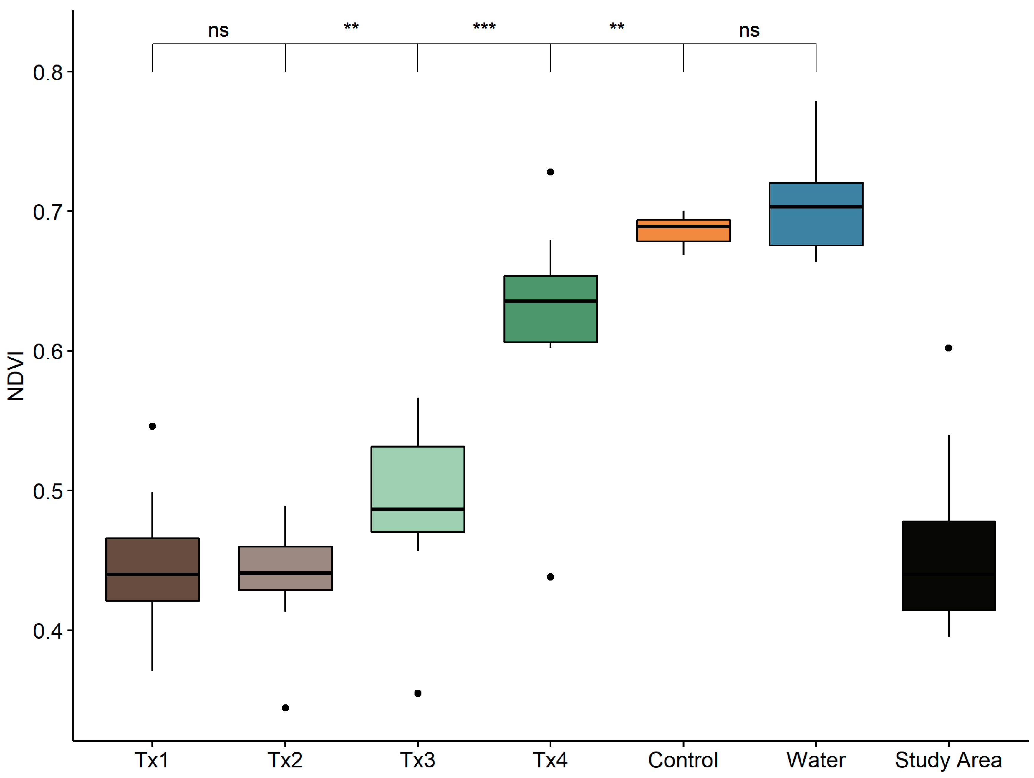
3.1. Detectability of Plant Water Status Over GSD and Time

Leaf water content samples for all treatments (Tx1, Tx2, Tx3, Tx4, C, and W) and pre-dawn and midday leaf water potential for treatments Tx3, Tx4, C, and W are shown in Table 2.
The relationship between flying height (and GSD) and time of day on detectability of leaf water status NDVI and NDRE values is plotted in Figure 2. Spectral indices vary with spatial resolution for several reasons, including the fact that lighting changes throughout the day, as well as leaf moisture. While it is possible to separate treatments and control at all resolutions (i.e., 2.2–8.7 cm GSD), the best separation between all treatments, including the water and control was at 2.2 cm and 4.3 cm GSD flown at altitude 30 m and 60 m, for both NDVI and NDRE (Figure 2a,b). At slightly coarser resolutions (7.2 cm and 8.7 cm GSD) the difference between control and water was less pronounced. NDVI and NDRE values by time of day are shown in Figure 2c. The best separation between treatments was found in the morning imagery for NDVI (between 10:00 and 12:00), and in the early morning for NDRE (between 8:00 and 10:00). The drier plots (e.g., Tx1 and Tx2) were less separable as the day progressed within both indices. The NDVI for Tx4 declined throughout the day, as we would expect, given this treatment had been enacted one day prior to the flights represented.

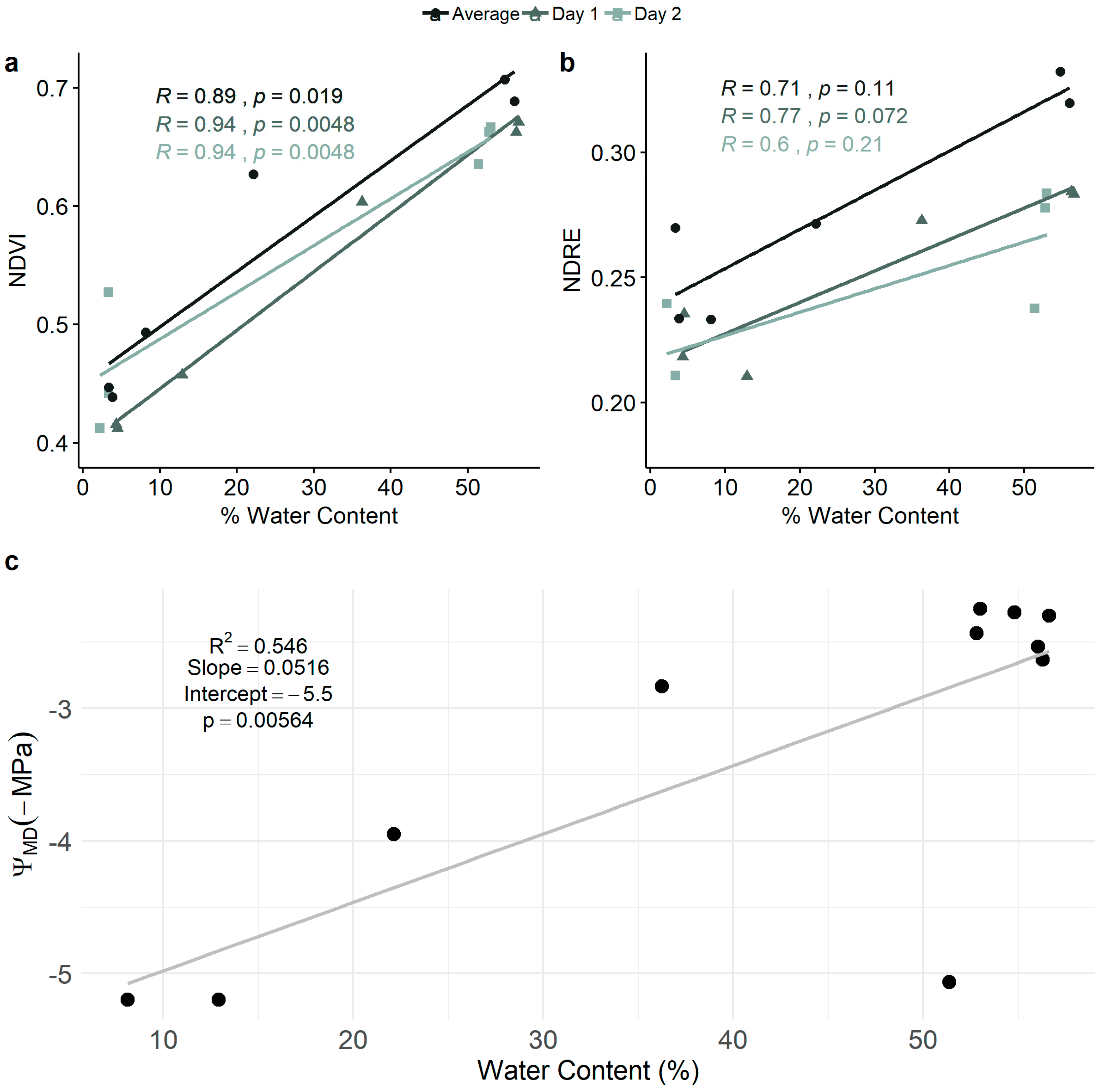
3.2. Relationships Among NDVI, NDRE, Leaf Water Content, and Leaf Water Potential

NDVI showed a statistically strong positive correlation with leaf water content. NDVI values from Day 1 and Day 2 correlated well with percent water content (rs = 0.94 for both days), and the average of all flights and leaf water content was associated with a slightly weaker yet statistically significant correlation of rs = 0.89 (Figure 3a). A weak correlation was found with NDRE and leaf water content (rs for Day 1, Day 2, and overall were 0.77, 0.60, and 0.71, respectively) (Figure 3b), therefore we present the rest of the results with NDVI. A simple linear regression was calculated to predict mid-day water potential based on water content. A significant regression equation was found with an R2 of 0.546 (Figure 3c). Leaf water potential decreased by 0.0516 (MPa) for each percent of water content. The regression was much stronger when Tx4 from Day 2 was removed as an outlier, resulting in an R2 of 0.921 (Figure S1).
The distribution of NDVI and NDRE for all resampled flights (n = 12, 8.7 cm) by treatment and in the overall study area is shown in Figure 4 and Figure S2 and Figure S3. Statistically significant differences were found in the NDVI values between Tx2 and Tx3, between Tx3 and Tx4, and between Tx4 and the control. Nonsignificant differences were found between Tx1 and Tx2, as well as the control and the water treatment (see Figure S2 for NDRE).

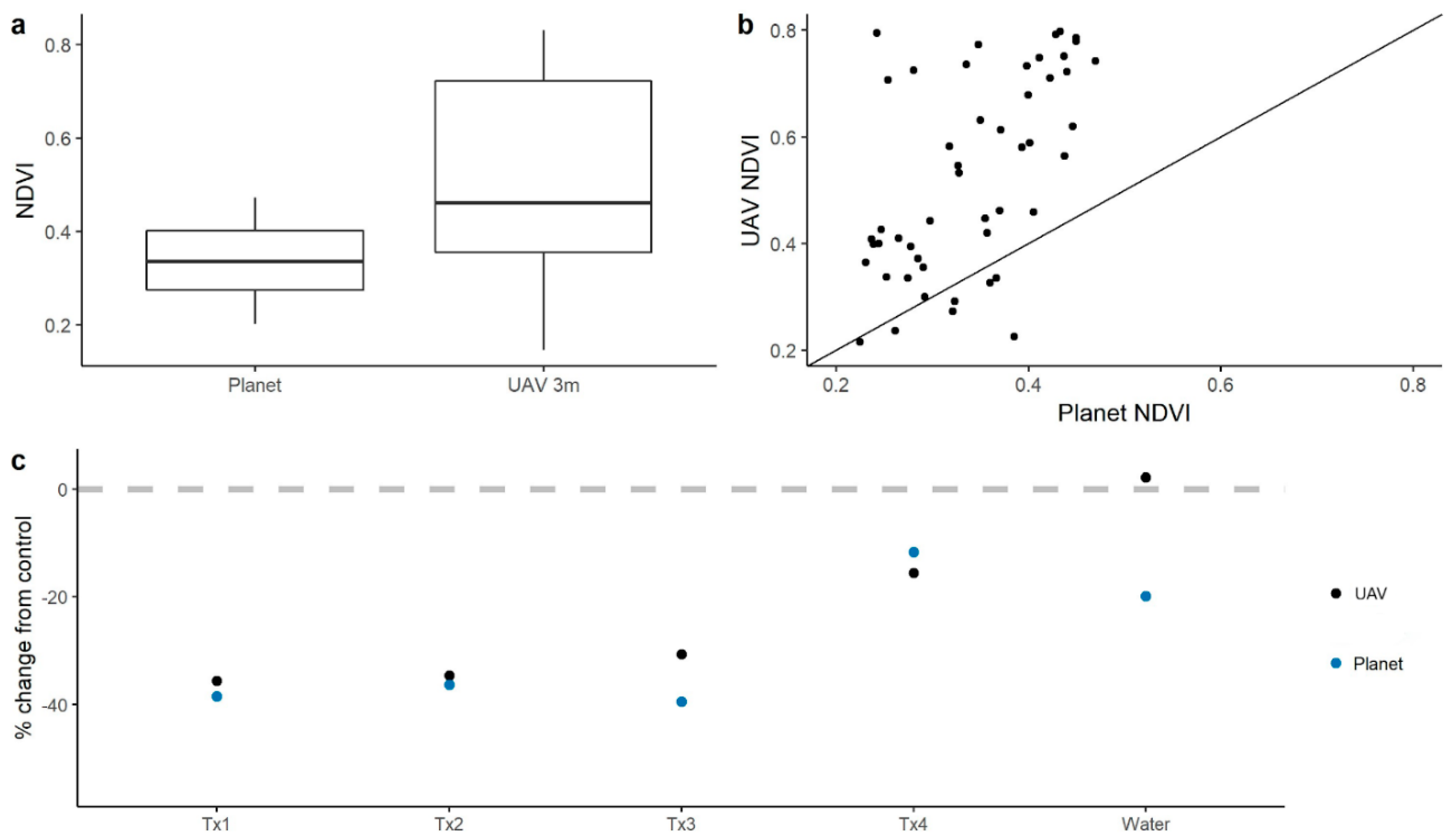
3.3. Scaling behavior of spectral indices

Our third objective was to explore how the relationship between indices and water status changed when the imagery was scaled to the coarser resolutions provided by satellites (Figure S4). Because our study area is small, only imagery from PlanetScope was used in the scaling experiment.
Assessing the distribution of pixels within the study area between the resampled UAV NDVI data (n = 35) and the NDVI derived from Planet (n = 35) (Figure 5a), we found that the range in NDVI values was much smaller for the PlanetScope data, with values across the study area ranging from 0.2 to 0.5. The resampled UAV NDVI pixel values contained more spectral information, suggesting higher spectral sensitivity of the MicaSense RedEdge narrow-band sensor in comparison with PlantScope’s sensor. A narrow-band sensor such as the RedEdge can provide more detailed information by capturing a more precise measurement of specific wavelengths (see Figure S5). Therefore, the spectral sensitivity of the sensor was preserved despite the change in spatial resolution. We found a positive correlation between the UAV NDVI and Planet NDVI, spearman’s rho statistic (rs) = 0.64, p = < 0.001(Figure 5b, Figure S6). The UAV NDVI values trended higher than the Planet NDVI values, which is consistent with higher sensitivity in the MicaSense RedEdge red and infrared spectral bands (Figure S5). We found that Planet data was able to capture an overall trend in treatments (i.e., able to detect healthy green vegetation from dead dry vegetation), even when treatments were represented by single pixels (Figure 5c). However, PlanetScope data was not able to capture subtle changes in water content (e.g., the water treatment had lower NDVI than the control).

4. Discussion

UAVs are increasingly being used to map natural and agricultural vegetation [43] due to their precision and flexibility [56]: UAVs allow the use of a range of cameras, control over ground sample distance, and the ability to precisely control the timing of image acquisition. Because of the ability to acquire data throughout the day, imagery from UAVs can offer very precise and new insights into the dynamics of land surface behavior at detailed spatial scales. Scientific interests such as phenology, changes in transpiration, plant water status, and carbon fluxes can be studied at unprecedented temporal resolutions (e.g., hourly or daily), potentially creating hypertemporal vegetation products for input into ecosystem models and new insights into ecosystem behavior. For example, Malbéteau et al. [57] explored diurnal temperature dynamics of grass and maize canopies in Saudi Arabia with varying water status levels at ultra-high spatial resolution (0.02 m). The use of UAVs allowed for fine temporal characterization of plant–water relations, as leaf skin temperature is strongly coupled with stomatal conductance and related to transpiration rates [58]. Several papers focusing on orchards in Spain showcase the ability of UAV-based hyperspectral imagery (and the PRI index in particular) to relate diurnal changes in plant water content to measures in the field at the time of each image acquisition [59,60].
Despite increasing spatiotemporal resolutions to understand variations in plant water relations, capturing accurate and meaningful data from UAVs and their associated sensors can be difficult. Key error sources associated with UAV data collection and processing, such as solar angle, weather conditions, geolocation, and radiometric calibration, can all influence the accuracy of the calculated vegetation indices [61]. In our study we found variations in calculated indices of NDVI and NDRE over the course of a day and varying solar angles. We found that NDVI was best able to capture differences across our treatments between 10:00 and 12:00, while the best differentiation in NDRE slightly earlier in the day (9:00). Studies have reported minimum values for vegetation indices at solar noon in areas with LAI (leaf area index) of 0.5–2, and data collected during the traditionally used “high sun″ condition with lower predictive capability than at oblique sun angles (solar zenith angle (SZA) > 40°) [62]. Our study didn’t observe the lowest vegetation index values at peak sun conditions; however, differences across treatments were more accurately captured at larger solar zenith angles earlier in the day. Additionally, the spatial resolution influences the detectability of changes in water condition as well as differences between treatments, therefore, determining the appropriate resolution imagery in which to disentangle these differences is important.
When focusing on plant water relations, commercial grade multispectral cameras are very useful, particularly when they have both red edge and NIR bands. We found complementarity between and nonredundant information content provided by both NDVI and NDRE. Both measures were able to identify moisture deficit in plants and distinguish them from control and watered plants; however, NDVI was better able to distinguish between treatments than NDRE and was more positively correlated with field measurements of leaf water content than NDRE. These results highlight the consistent utility of NDVI in water deficit and plant health studies. Despite these mixed results, it is likely that applications for and evaluation of red edge sensors will grow. As recently as 2014, red-edge cameras were not routinely used for vegetation mapping [63], however, now there are several satellite-based sensors that include one or more red-edge bands: the Sentinel-2 satellite (3 bands between 700 and 790 nm, 20 m GSD), RapidEye (690–730 nm, 6.5 m GSD), and WorldView-3 (but not WorldView-4) (705–745 nm, 1.4 m GSD), and UAV mounted commercial off-the-shelf multispectral cameras with red edge sensitivity are increasingly popular [47]. Our results suggest a more thorough evaluation of the application and underlying physiological responses to changes in the red-edge spectra is needed.
However, assessing the applicability of vegetation indices to represent physiological difference in plants must be continually calibrated. Yan et al. [64] articulated the difficulty in using measures of greenness including NDVI as a proxy for productivity. They concluded that because greenness changes more slowly than plant physiological function, relationships between remotely sensed vegetation indices of drought-tolerant species and gross primary productivity break down on short timescales and decouple during periods of water deficit [64,65]. Consequently, there remains a critical need to calibrate vegetation indices across ecosystems and across time to enable robust remote sensing of plant physiology. Our experiment showed the potential for linking field-based water content and water potential measurements to NDVI and NDRE, with particularly strong correlations between water content and NDVI. Several studies linking plant water content to spectral indices focus on reflected radiation in the 800 nm–2500 nm range from custom sensors or hyperspectral sensors [66,67]. However, the use of such systems is limited due to their high cost and fewer platforms that carry them. With the increased use of off-the-shelf multispectral sensors in environmental and agricultural research, there is a need for continued evaluation of vegetation indices that can be derived from narrow-band multispectral sensors such as MicaSense RedEdge and Sequoia. For good overviews of vegetation indices derived from UAV data see [1,68].
Connecting relative water content, which is an indirect measurement of a change in water status, to physiological determinants of water status such as water potential is still needed. Here we showed that water potential can be derived from estimates of water content with an R2 of 54% (92% with outliers removed), however this is a small sample size, and although the relationship appears encouraging, we do not have enough information to conclude that water potential can reliability be inferred from common vegetation indices such as NDVI or NDRE. NDVI does detect fine scale variations in water deficit, as shown in Figure 4, apart from treatments that were extremely dry (e.g., Tx1 and Tx2) and treatments with fine scale variation (control vs. water). Despite these limitations, UAVs appear to be a useful tool for detecting small-scale changes in water status (content and water potential).
The retrieval of spectral signatures and their association with underlying physiological processes remains a research challenge but also an opportunity, especially in scaling research. Calibration experiments such as the one reported on here are critical to develop robust scaling relationships. In this paper, we show that the derived NDVI values from UAVs and PlanetScope CubeSat imagery across treatments are largely consistent with important differences, particularly in their sensitivity to subtle changes to water content (control and water). Studies have shown that vegetation indices, such as NDVI, can be significantly affected by differences in spectral bandwidth [61,69]. The spectral range of the red band has been found to be of importance to NDVI. Therefore, investment in increased spectral resolution rather than increased spatial resolution in the development of CubeSats may be more important for understanding patterns in vegetation health and water content. In line with our results, several studies document a lower top of atmosphere NDVI compared with NDVI at the surface due to the atmospheric scattering effect [70,71]; however, recent improvements in PlanetScope’s surface reflectance products should minimize this effect [71]. Additionally, acquiring UAV imagery that can be used to scale across sensors, space, and time can be challenging, due to differences between sensors and sensor units, ambient weather, and lighting conditions [61,63].
Narrowband hyperspectral imagery and derived indices are also appropriate for detecting daily changes in plant moisture status, but not yet commonly practical using commercial UAV cameras. Most notably among these is the photochemical reflectance index (PRI), which uses bands at 532 nm and 570 nm and requires a hyperspectral imaging camera [59,60]. PRI was developed to capture diurnal changes in the xanthophyll cycle of leaves and canopies, which contributes to a plant’s ability to efficiently disperse light energy for photosynthesis [72]. Because water limitation affects the light-harvesting capacities and photosynthetic pathways within the leaves of a plant, PRI has become an appropriate index with which to detect the effects of rapid changes in plant health due to lack of water. Additionally, evergreen species, such as coyote brush, alter their chlorophyll:carotenoid ratios in response to water or temperature availability, and this can be detected with PRI on a seasonal or daily timescale [73]. NDVI, however, may be less suited for diurnal detection of water stress impacts on vegetation greenness or photosynthetic capabilities in evergreens, because canopy reflectance remains relatively stable even throughout the beginning and end of a season, when species alter rates of photosynthesis and have access to varying amounts of water. Furthermore, nuanced differences in photosynthetic downregulation during brief or sudden disturbances may not be captured by NDVI. While NDVI is effective in detecting longer-term changes in photosynthesis (such as new growth and leaf development), PRI is more suitable for subtle changes in evergreen leaf pigmentation. However, over longer time scales, NDVI and PRI can be used together to understand rates of photosynthesis, carbon fixation, and net primary production in a plant based on the combination of greenness and light-use efficiency models [72]. New work also highlights the ability to measure solar-induced fluorescence via narrowband remote sensing. About 1% of solar energy captured by plants is re-emitted by chlorophyll as fluorescence. The amount of fluorescence emission is a direct indicator of the photosynthetic activity of a plant and also provides indirect information about the plant stress [74]. Remote sensing of solar-induced fluorescence requires very narrow spectral bands (~0.05 nm) around 690 nm and 760 nm [67,75].

5. Conclusions

We conducted a water exclusion experiment over one week to plots of Baccharis pilularis (coyote brush) at the Blue Oak Ranch Reserve (BORR) near San Jose, California. We monitored the experiment at several altitudes with nearly hourly data collections over two days to determine: (1) spatial and temporal thresholds at which water limitation in plants could be detected via common spectral indices (NDVI and NDRE); (2) relationships between spectral and physiological responses to plant water deficit; and (3) how coarser resolution imagery provided by PlanetScope data compared with UAV-collected imagery. We found the best separation between treatments at higher resolution (lower flying height), and the best separation between treatments in the morning (NDVI) and early morning (NDRE). Overall, most treatments could be differentiated spectrally from each other and from the control, with some exceptions. For example, it was difficult to separate the driest plots (Tx1 and Tx2) using NDVI. These results suggest that while there are important differences between NDVI and NDRE across treatments, there also exists some complementarity between NDVI and NDRE indices that needs further evaluation. We found strong relationships between NDVI and leaf water content (highest r = 0.94).
When comparing PlanetScope to UAV imagery collected at the same time, we found that PlanetScope data was able to capture the overall trend in treatments (i.e., able to detect healthy green vegetation from dead dry vegetation), even when treatments were represented by single pixels. However, PlanetScope data was not able to capture subtle changes in water content. Although there was a positive correlation between NDVI derived from the UAV and PlanetScope, the UAV imagery captured a larger spectral range, suggesting a greater spectral sensitivity to plant responses to water deficit with the UAV camera than with the PlanetScope imagery. In this case a narrow-band sensor such as the RedEdge provided more detailed information by capturing a more precise measurement of specific wavelengths than did the PlanetScope sensor.
What differentiates data collected from UAVs from data collected by high-resolution satellite sensors is their ability to collect data on demand, at high temporal resolution, and with multiple sensor payloads. Because of this and their increasing popularity, more experiments that evaluate the relationship between direct field measurements and camera sensitivity are needed. Scaling simple vegetation indices from UAVs to CubeSats will increase our ability to translate field-based physiology measurements to landscape or regional scales.

Supplementary Materials

The following are available online at https://www.mdpi.com/2072-4292/11/16/1853/s1, Figure S1: A simple linear regression was calculated to predict mid-day water potential on the basis of water content. Data gathered for Tx4 from Day 2 (outlier) was removed to further assess fit. A significant regression equation was found with an R2 of 0.921. Leaf water potential decreased 0.0585 (MPa) for each percent water content; Figure S2: Spectral index value for all pixels (Day 1 and Day 2) by treatment: NDRE values. Difference between pairs of treatments determined from Wilcox test are indicated at the top of each pair: ns = not significant at 0.05 significance level (p > 0.05), *: p ≤ 0.05, **: p ≤ 0.01, ***: p ≤ 0.001; Figure S3: Density plot of distribution of NDVI vs. NDRE values for a) all pixels within all n = 12 UAV flights, b) all pixels for all flights for each treatment. Colors are representative of similarity in values, with blue colors showing lower correlation, and red colors showing higher correlation between the values of the two indices; Figure S4: General study area before and after treatments for UAV and PlanetScope; Figure S5: Band wavelengths (nm) of the MicaSense Red-Edge Sensor with PlanetScope and RapidEye sensors; Figure S6: Spearman’s rho statistic (rs) = 0.64 positive correlation between UAV NDVI and PlanetScope NDVI. Table S1: Pixel counts for the overall study area and each treatment at 4.45 cm GSD or 60 m flying altitude.

Author Contributions

Conceptualization: T.E.D., K.E., M.K.; Data curation: K.E., S.H.; Formal analysis, K.E., C.K.; Methodology: K.E., T.E.D., M.K., S.H.; Project administration: T.E.D., K.E., M.K.; Validation, K.E., M.K.; Writing—original draft, K.E., M.K., C.K., T.E.D.; Writing—review & editing, K.E., C.K., M.K., S.H., T.E.D.

Funding

This research was funded by the Betty & Gordon Moore Foundation under the project title: The California Heartbeat Initiative.

Acknowledgments

The authors would like to acknowledge the financial support provided by the Betty and Gordon Moore Foundation. We also thank Zac Harlow and Zac Tuthill for helping us carrying out the experimental design. Members of the California Heartbeat Initiative-Freshwater program, David Ackerly, Collin Bode, Becca Fenwick, Peggy Fiedler, Kerri Johnson and Jim Norris provided key assistance and thoughtful help.

Conflicts of Interest

The authors declare no conflict of interest.

References

  1. Govender, M.; Govender, P.J.; Weiersbye, I.M.; Witkowski, E.T.F.; Ahmed, F. Review of commonly used remote sensing and ground-based technologies to measure plant water stress. Water SA 2009, 35. [Google Scholar] [CrossRef] [Green Version]
  2. Donovan, L.A.; Richards, J.H.; Linton, M.J. Magnitude and Mechanisms of Disequilibrium between Predawn Plant and Soil Water Potentials. Ecology 2003, 84, 463–470. [Google Scholar] [CrossRef]
  3. Ambrose, A.R.; Baxter, W.L.; Martin, R.E.; Francis, E.; Asner, G.P.; Nydick, K.R.; Dawson, T.E. Leaf- and crown-level adjustments help giant sequoias maintain favorable water status during severe drought. For. Ecol. Manag. 2018, 419–420, 257–267. [Google Scholar] [CrossRef]
  4. Allen, C.D.; Macalady, A.K.; Chenchouni, H.; Bachelet, D.; McDowell, N.; Vennetier, M.; Kitzberger, T.; Rigling, A.; Breshears, D.D.; Hogg, E.H.; et al. A global overview of drought and heat-induced tree mortality reveals emerging climate change risks for forests. For. Ecol. Manag. 2010, 259, 660–684. [Google Scholar] [CrossRef] [Green Version]
  5. McDowell, N.; Pockman, W.T.; Allen, C.D.; Breshears, D.D.; Cobb, N.; Kolb, T.; Plaut, J.; Sperry, J.; West, A.; Williams, D.G.; et al. Mechanisms of plant survival and mortality during drought: Why do some plants survive while others succumb to drought? New Phytol. 2008, 178, 719–739. [Google Scholar] [CrossRef] [PubMed]
  6. Mencuccini, M.; Manzoni, S.; Christoffersen, B. Modelling water fluxes in plants: From tissues to biosphere. New Phytol. 2019, 222, 1207–1222. [Google Scholar] [CrossRef] [PubMed]
  7. Dennison, P.E.; Roberts, D.A.; Thorgusen, S.R.; Regelbrugge, J.C.; Weise, D.; Lee, C. Modeling seasonal changes in live fuel moisture and equivalent water thickness using a cumulative water balance index. Remote Sens. Environ. 2003, 88, 442–452. [Google Scholar] [CrossRef]
  8. Emery, N.C.; D’Antonio, C.M.; Still, C.J. Fog and live fuel moisture in coastal California shrublands. Ecosphere 2018, 9, e02167. [Google Scholar] [CrossRef]
  9. Millar, C.I.; Westfall, R.D.; Delany, D.L.; Bokach, M.J.; Flint, A.L.; Flint, L.E. Forest mortality in high-elevation whitebark pine (Pinus albicaulis) forests of eastern California, USA; influence of environmental context, bark beetles, climatic water deficit, and warming. Can. J. For. Res. 2012, 42, 749–765. [Google Scholar] [CrossRef]
  10. McIntyre, P.J.; Thorne, J.H.; Dolanc, C.R.; Flint, A.L.; Flint, L.E.; Kelly, M.; Ackerly, D.D. Twentieth-century shifts in forest structure in California: Denser forests, smaller trees, and increased dominance of oaks. Proc. Natl. Acad. Sci. USA 2015, 112, 1458–1463. [Google Scholar] [CrossRef] [Green Version]
  11. Asbjornsen, H.; Goldsmith, G.R.; Alvarado-Barrientos, M.S.; Rebel, K.; Van Osch, F.P.; Rietkerk, M.; Chen, J.; Gotsch, S.; Tobón, C.; Geissert, D.R.; et al. Ecohydrological advances and applications in plant–water relations research: A review. J. Plant Ecol. 2011, 4, 3–22. [Google Scholar] [CrossRef]
  12. Asner, G.P.; Brodrick, P.G.; Anderson, C.B.; Vaughn, N.; Knapp, D.E.; Martin, R.E. Progressive forest canopy water loss during the 2012–2015 California drought. Proc. Natl. Acad. Sci. USA 2016, 113, E249–E255. [Google Scholar] [CrossRef] [PubMed]
  13. Paz-Kagan, T.; Brodrick, P.G.; Vaughn, N.R.; Das, A.J.; Stephenson, N.L.; Nydick, K.R.; Asner, G.P. What mediates tree mortality during drought in the southern Sierra Nevada? Ecol. Appl. 2017, 27, 2443–2457. [Google Scholar] [CrossRef] [PubMed]
  14. McLaughlin, B.C.; Ackerly, D.D.; Klos, P.Z.; Natali, J.; Dawson, T.E.; Thompson, S.E. Hydrologic refugia, plants, and climate change. Glob. Chang. Biol. 2017, 23, 2941–2961. [Google Scholar] [CrossRef] [PubMed] [Green Version]
  15. Stephens, S.L.; Collins, B.M.; Biber, E.; Fulé, P.Z. US federal fire and forest policy: Emphasizing resilience in dry forests. Ecosphere 2016, 7, e01584. [Google Scholar] [CrossRef]
  16. Westerling, A.L.; Hidalgo, H.G.; Cayan, D.R.; Swetnam, T.W. Warming and earlier spring increase western U.S. forest wildfire activity. Science 2006, 313, 940–943. [Google Scholar] [CrossRef] [PubMed]
  17. Westerling, A.L.; Bryant, B.P. Climate change and wildfire in California. Clim. Chang. 2008, 87, 231–249. [Google Scholar] [CrossRef]
  18. Boisramé, G.F.S.; Thompson, S.E.; Kelly, M.; Cavalli, J.; Wilkin, K.M.; Stephens, S.L. Vegetation change during 40years of repeated managed wildfires in the Sierra Nevada, California. For. Ecol. Manag. 2017, 402, 241–252. [Google Scholar] [CrossRef]
  19. Mazer, S.J.; Gerst, K.L.; Matthews, E.R.; Evenden, A. Species-specific phenological responses to winter temperature and precipitation in a water-limited ecosystem. Ecosphere 2015, 6, 1–27. [Google Scholar] [CrossRef]
  20. Gausman, H.W. Reflectance of leaf components. Remote Sens. Environ. 1977, 6, 1–9. [Google Scholar] [CrossRef]
  21. Byrd, K.B.; O’Connell, J.L.; Di Tommaso, S.; Kelly, M. Evaluation of sensor types and environmental controls on mapping biomass of coastal marsh emergent vegetation. Remote Sens. Environ. 2014, 149, 166–180. [Google Scholar] [CrossRef]
  22. Jensen, J.R. Biophysical Remote Sensing. Ann. Assoc. Am. Geogr. 1983, 73, 111–132. [Google Scholar] [CrossRef]
  23. Tuxen, K.; Schile, L.; Stralberg, D.; Siegel, S.; Parker, T.; Vasey, M.; Callaway, J.; Kelly, M. Mapping changes in tidal wetland vegetation composition and pattern across a salinity gradient using high spatial resolution imagery. Wetl. Ecol. Manag. 2011, 19, 141–157. [Google Scholar] [CrossRef]
  24. Pettorelli, N.; Vik, J.O.; Mysterud, A.; Gaillard, J.-M.; Tucker, C.J.; Stenseth, N.C. Using the satellite-derived NDVI to assess ecological responses to environmental change. Trends Ecol. Evol. 2005, 20, 503–510. [Google Scholar] [CrossRef] [PubMed]
  25. Fung, T.; Siu, W. Environmental quality and its changes, an analysis using NDVI. Int. J. Remote Sens. 2000, 21, 1011–1024. [Google Scholar] [CrossRef]
  26. Nouri, H.; Beecham, S.; Anderson, S.; Nagler, P. High Spatial Resolution WorldView-2 Imagery for Mapping NDVI and Its Relationship to Temporal Urban Landscape Evapotranspiration Factors. Remote Sens. 2014, 6, 580–602. [Google Scholar] [CrossRef] [Green Version]
  27. Viña, A.; Gitelson, A.A.; Nguy-Robertson, A.L.; Peng, Y. Comparison of different vegetation indices for the remote assessment of green leaf area index of crops. Remote Sens. Environ. 2011, 115, 3468–3478. [Google Scholar] [CrossRef]
  28. Horler, D.N.H.; Dockray, M.; Barber, J. The red edge of plant leaf reflectance. Int. J. Remote Sens. 1983, 4, 273–288. [Google Scholar] [CrossRef]
  29. Horler, D.N.H.; Dockray, M.; Barber, J.; Barringer, A.R. Red edge measurements for remotely sensing plant chlorophyll content. Adv. Space Res. 1983, 3, 273–277. [Google Scholar] [CrossRef]
  30. Ju, C.-H.; Tian, Y.-C.; Yao, X.; Cao, W.-X.; Zhu, Y.; Hannaway, D. Estimating Leaf Chlorophyll Content Using Red Edge Parameters. Pedosphere 2010, 20, 633–644. [Google Scholar] [CrossRef]
  31. Mutanga, O.; Skidmore, A.K. Narrow band vegetation indices overcome the saturation problem in biomass estimation. Int. J. Remote Sens. 2004, 25, 3999–4014. [Google Scholar] [CrossRef]
  32. Filella, I.; Penuelas, J. The red edge position and shape as indicators of plant chlorophyll content, biomass and hydric status. Int. J. Remote Sens. 1994, 15, 1459–1470. [Google Scholar] [CrossRef]
  33. Cui, Z.; Kerekes, J.P. Potential of Red Edge Spectral Bands in Future Landsat Satellites on Agroecosystem Canopy Green Leaf Area Index Retrieval. Remote Sens. 2018, 10, 1458. [Google Scholar] [CrossRef]
  34. Eitel, J.U.H.; Vierling, L.A.; Litvak, M.E.; Long, D.S.; Schulthess, U.; Ager, A.A.; Krofcheck, D.J.; Stoscheck, L. Broadband, red-edge information from satellites improves early stress detection in a New Mexico conifer woodland. Remote Sens. Environ. 2011, 115, 3640–3646. [Google Scholar] [CrossRef]
  35. Gitelson, A.; Merzlyak, M.N. Spectral Reflectance Changes Associated with Autumn Senescence of Aesculus hippocastanum L. and Acer platanoides L. Leaves. Spectral Features and Relation to Chlorophyll Estimation. J. Plant Physiol. 1994, 143, 286–292. [Google Scholar] [CrossRef]
  36. Sims, D.A.; Gamon, J.A. Relationships between leaf pigment content and spectral reflectance across a wide range of species, leaf structures and developmental stages. Remote Sens. Environ. 2002, 81, 337–354. [Google Scholar] [CrossRef]
  37. Katsoulas, N.; Elvanidi, A.; Ferentinos, K.P.; Kacira, M.; Bartzanas, T.; Kittas, C. Crop reflectance monitoring as a tool for water stress detection in greenhouses: A review. Biosyst. Eng. 2016, 151, 374–398. [Google Scholar] [CrossRef]
  38. Behmann, J.; Steinrücken, J.; Plümer, L. Detection of early plant stress responses in hyperspectral images. ISPRS J. Photogramm. Remote Sens. 2014, 93, 98–111. [Google Scholar] [CrossRef]
  39. Wang, R.; Cherkauer, K.; Bowling, L. Corn Response to Climate Stress Detected with Satellite-Based NDVI Time Series. Remote Sens. 2016, 8, 269. [Google Scholar] [CrossRef]
  40. Clevers, J.G.P.W.; Gitelson, A.A. Remote estimation of crop and grass chlorophyll and nitrogen content using red-edge bands on Sentinel-2 and -3. Int. J. Appl. Earth Obs. Geoinf. 2013, 23, 344–351. [Google Scholar] [CrossRef]
  41. Pu, R.; Kelly, M.; Anderson, G.L.; Gong, P. Using CASI Hyperspectral Imagery to Detect Mortality and Vegetation Stress Associated with a New Hardwood Forest Disease. Photogramm. Eng. Remote Sens. 2008, 74, 65–75. [Google Scholar] [CrossRef] [Green Version]
  42. Pu, R.; Ge, S.; Kelly, N.M.; Gong, P. Spectral absorption features as indicators of water status in coast live oak (Quercus agrifolia) leaves. Int. J. Remote Sens. 2003, 24, 1799–1810. [Google Scholar] [CrossRef]
  43. Hogan, S.D.; Kelly, M.; Stark, B.; Chen, Y. Unmanned aerial systems for agriculture and natural resources. Calif. Agric. 2017, 71, 5–14. [Google Scholar] [CrossRef]
  44. Hunt, E.R.; Daughtry, C.S.T. What good are unmanned aircraft systems for agricultural remote sensing and precision agriculture? Int. J. Remote Sens. 2018, 39, 5345–5376. [Google Scholar] [CrossRef]
  45. Gago, J.; Douthe, C.; Coopman, R.E.; Gallego, P.P.; Ribas-Carbo, M.; Flexas, J.; Escalona, J.; Medrano, H. UAVs challenge to assess water stress for sustainable agriculture. Agric. Water Manag. 2015, 153, 9–19. [Google Scholar] [CrossRef]
  46. Zhao, T.; Stark, B.; Chen, Y.; Ray, A.; Doll, D. More Reliable Crop Water Stress Quantification Using Small Unmanned Aerial Systems (sUAS). IFAC PapersOnLine 2016, 49, 409–414. [Google Scholar] [CrossRef]
  47. Jorge, J.; Vallbé, M.; Soler, J.A. Detection of irrigation inhomogeneities in an olive grove using the NDRE vegetation index obtained from UAV images. Eur. J. Remote Sens. 2019, 52, 169–177. [Google Scholar] [CrossRef] [Green Version]
  48. Wahab, I.; Hall, O.; Jirström, M. Remote Sensing of Yields: Application of UAV Imagery-Derived NDVI for Estimating Maize Vigor and Yields in Complex Farming Systems in Sub-Saharan Africa. Drones 2018, 2, 28. [Google Scholar] [CrossRef]
  49. Díaz-Delgado, R.; Ónodi, G.; Kröel-Dulay, G.; Kertész, M. Enhancement of Ecological Field Experimental Research by Means of UAV Multispectral Sensing. Drones 2019, 3, 7. [Google Scholar] [CrossRef]
  50. Dunford, R.; Michel, K.; Gagnage, M.; Piégay, H.; Trémelo, M.-L. Potential and constraints of Unmanned Aerial Vehicle technology for the characterization of Mediterranean riparian forest. Int. J. Remote Sens. 2009, 30, 4915–4935. [Google Scholar] [CrossRef]
  51. Hernández-Clemente, R.; Navarro-Cerrillo, R.M.; Zarco-Tejada, P.J. Carotenoid content estimation in a heterogeneous conifer forest using narrow-band indices and PROSPECT+ DART simulations. Remote Sens. Environ. 2012, 127, 298–315. [Google Scholar] [CrossRef]
  52. Scholander, P.F.; Bradstreet, E.D.; Hemmingsen, E.A.; Hammel, H.T. Sap Pressure in Vascular Plants: Negative hydrostatic pressure can be measured in plants. Science 1965, 148, 339–346. [Google Scholar] [CrossRef] [PubMed]
  53. Pix4D Software. Available online: https://pix4d.com/ (accessed on 7 August 2018).
  54. Kerby, D.S. The Simple Difference Formula: An Approach to Teaching Nonparametric Correlation. Compr. Psychol. 2014, 3, 11-IT. [Google Scholar] [CrossRef]
  55. Planet Team. Planet Team. Planet Application Program Interface. In Space for Life on Earth; Planet Team: San Francisco, CA, USA, 2017. [Google Scholar]
  56. Shiklomanov, A.N.; Bradley, B.A.; Dahlin, K.M.; Fox, A.M.; Gough, C.M.; Hoffman, F.M.; Middleton, E.M.; Serbin, S.P.; Smallman, L.; Smith, W.K. Enhancing global change experiments through integration of remote-sensing techniques. Front. Ecol. Environ. 2019, 11, 138. [Google Scholar] [CrossRef]
  57. Malbéteau, Y.; Parkes, S.; Aragon, B.; Rosas, J.; McCabe, M. Capturing the Diurnal Cycle of Land Surface Temperature Using an Unmanned Aerial Vehicle. Remote Sens. 2018, 10, 1407. [Google Scholar] [CrossRef]
  58. Damm, A.; Paul-Limoges, E.; Haghighi, E.; Simmer, C.; Morsdorf, F.; Schneider, F.D.; van der Tol, C.; Migliavacca, M.; Rascher, U. Remote sensing of plant-water relations: An overview and future perspectives. J. Plant Physiol. 2018, 227, 3–19. [Google Scholar] [CrossRef] [PubMed]
  59. Zarco-Tejada, P.J.; González-Dugo, V.; Williams, L.E.; Suárez, L.; Berni, J.A.J.; Goldhamer, D.; Fereres, E. A PRI-based water stress index combining structural and chlorophyll effects: Assessment using diurnal narrow-band airborne imagery and the CWSI thermal index. Remote Sens. Environ. 2013, 138, 38–50. [Google Scholar] [CrossRef]
  60. Suárez, L.; Zarco-Tejada, P.J.; Sepulcre-Cantó, G.; Pérez-Priego, O.; Miller, J.R.; Jiménez-Muñoz, J.C.; Sobrino, J. Assessing canopy PRI for water stress detection with diurnal airborne imagery. Remote Sens. Environ. 2008, 112, 560–575. [Google Scholar] [CrossRef]
  61. Assmann, J.J.; Kerby, J.T.; Cunliffe, A.M.; Myers-Smith, I.H. Vegetation monitoring using multispectral sensors—Best practices and lessons learned from high latitudes. J. Unmanned Veh. Syst. 2019, 7, 54–75. [Google Scholar] [CrossRef]
  62. Middleton, E.M. Solar zenith angle effects on vegetation indices in tallgrass prairie. Remote Sens. Environ. 1991, 38, 45–62. [Google Scholar] [CrossRef]
  63. Salamí, E.; Barrado, C.; Pastor, E. UAV Flight Experiments Applied to the Remote Sensing of Vegetated Areas. Remote Sens. 2014, 6, 11051–11081. [Google Scholar] [CrossRef] [Green Version]
  64. Yan, D.; Scott, R.L.; Moore, D.J.P.; Biederman, J.A.; Smith, W.K. Understanding the relationship between vegetation greenness and productivity across dryland ecosystems through the integration of PhenoCam, satellite, and eddy covariance data. Remote Sens. Environ. 2019, 223, 50–62. [Google Scholar] [CrossRef]
  65. Helman, D. Land surface phenology: What do we really “see″ from space? Sci. Total Environ. 2018, 618, 665–673. [Google Scholar] [CrossRef]
  66. Martin, R.E.; Asner, G.P.; Francis, E.; Ambrose, A.; Baxter, W.; Das, A.J.; Vaughn, N.R.; Paz-Kagan, T.; Dawson, T.; Nydick, K.; et al. Remote measurement of canopy water content in giant sequoias (Sequoiadendron giganteum) during drought. For. Ecol. Manag. 2018, 419–420, 279–290. [Google Scholar] [CrossRef]
  67. Zarco-Tejada, P.J.; González-Dugo, V.; Berni, J.A.J. Fluorescence, temperature and narrow-band indices acquired from a UAV platform for water stress detection using a micro-hyperspectral imager and a thermal camera. Remote Sens. Environ. 2012, 117, 322–337. [Google Scholar] [CrossRef]
  68. Pádua, L.; Vanko, J.; Hruška, J.; Adão, T.; Morais, R. UAS, sensors, and data processing in agroforestry: A review towards practical applications. Int. J. Remote Sens. 2017, 38, 2349–2391. [Google Scholar] [CrossRef]
  69. Rossi, M.; Niedrist, G.; Asam, S.; Tonon, G.; Tomelleri, E.; Zebisch, M. A Comparison of the Signal from Diverse Optical Sensors for Monitoring Alpine Grassland Dynamics. Remote Sens. 2019, 11, 296. [Google Scholar] [CrossRef]
  70. Trishchenko, A.P.; Cihlar, J.; Li, Z. Effects of spectral response function on surface reflectance and NDVI measured with moderate resolution satellite sensors. Remote Sens. Environ. 2002, 81, 1–18. [Google Scholar] [CrossRef]
  71. Liu, H.; Dahlgren, R.A.; Larsen, R.E.; Devine, S.M.; Roche, L.M.; O’Geen, A.T.; Wong, A.J.Y.; Covello, S.; Jin, Y. Estimating Rangeland Forage Production Using Remote Sensing Data from a Small Unmanned Aerial System (sUAS) and PlanetScope Satellite. Remote Sensing 2019, 11, 595. [Google Scholar] [CrossRef]
  72. Gamon, J.A.; Kovalchuck, O.; Wong, C.Y.S.; Harris, A.; Garrity, S.R. Monitoring seasonal and diurnal changes in photosynthetic pigments with automated PRI and NDVI sensors. Biogeosciences 2015, 12, 4149–4159. [Google Scholar] [CrossRef] [Green Version]
  73. Stylinski, C.; Gamon, J.; Oechel, W. Seasonal patterns of reflectance indices, carotenoid pigments and photosynthesis of evergreen chaparral species. Oecologia 2002, 131, 366–374. [Google Scholar] [CrossRef] [PubMed]
  74. Kalaji, H.M.; Jajoo, A.; Oukarroum, A.; Brestic, M.; Zivcak, M.; Samborska, I.A.; Cetner, M.D.; Łukasik, I.; Goltsev, V.; Ladle, R.J. Chlorophyll a fluorescence as a tool to monitor physiological status of plants under abiotic stress conditions. Acta Physiol. Plant 2016, 38, 102. [Google Scholar] [CrossRef]
  75. Porcar-Castell, A.; Tyystjärvi, E.; Atherton, J.; van der Tol, C.; Flexas, J.; Pfündel, E.E.; Moreno, J.; Frankenberg, C.; Berry, J.A. Linking chlorophyll a fluorescence to photosynthesis for remote sensing applications: Mechanisms and challenges. J. Exp. Bot. 2014, 65, 4065–4095. [Google Scholar] [CrossRef] [PubMed]
Figure 1. Experimental plot at Blue Oak Ranch Reserve (BORR): (a) study area location near San Jose, California, and range of B. pilularis; (b) experimental site from the ground; (c) detailed aerial depiction of experiment.
Remotesensing 11 01853 g001
Figure 2. (a) NDVI values and (b) NDRE values per treatment for flights with GSD of 2.2 cm, 4.3 cm, 7.2 cm, and 8.7 cm (flying height of 30m, 60m, 100m, and 120m); and (c) spectral index value per treatment over the course of eight flights in one day (resampled to 4.3 cm resolution). NDVI: normalized difference vegetation index. NDRE: normalized difference red edge index.
Remotesensing 11 01853 g002
Figure 3. (a) Relationship ((R = spearman’s rho statistic (rs)) between NDVI and water content at: 1pm on Day 1; 1pm on Day 2; and all values; (b) Relationship (R = spearman’s rho statistic (rs)) between NDRE and Water Content at: 1pm on Day 1; 1pm on Day 2; and all values; and (c) relationship (R-squared from linear regression) between plant water content and mid-day water potential (Note: the data point at −5 MPa and 52% water content is an anomaly and likely due to the timing of the treatment (immediately following cutting)).
Remotesensing 11 01853 g003
Figure 4. Spectral index value for all pixels (Day 1 and Day 2) by treatment: Difference between pairs of treatments determined from Wilcox test are indicated at the top of each pair: ns = not significant at 0.05 significance level (p > 0.05), *: p ≤ 0.05 **: p ≤ 0.01, ***: p ≤ 0.001.
Remotesensing 11 01853 g004
Figure 5. Scaling results comparing UAV data and PlanetScope data: (a) boxplot of NDVI for PlanetScope and UAV resampled to 3 m; (b) correlation between UAV NDVI and PlanetScope NDVI; and (c) % change from control in NDVI value for UAS raw value and PlanetScope.
Remotesensing 11 01853 g005
Table 1. Overview of UAV (unmanned aerial vehicles) flights flown on 25 July 2018 and 26 July 2018 with a MicaSense RedEdge multispectral camera at varying times and ground sampling distances (GSDs).
FlightDateTimeAltitudeGSD RedEdge (cm)
F125 July 201812:00120m8.81
F225 July 201813:15100m7.29
F325 July 201814:1030m2.26
F425 July 201815:1060m4.45
F526 July 201808:1760m4.47
F626 July 201809:3260m4.42
F726 July 201810:1360m4.48
F826 July 201811:1060m4.49
F926 July 201812:1060m4.71
F1026 July 201813:2460m4.42
F1126 July 201814:1060m4.40
F1226 July 201815:1060m4.36
Table 2. Acquired water content (WC) and water potential (WP) samples and averages for Day 1 (25 July) and Day 2 (26 July) for each treatment.
SamplesDay 1 WCDay 2 WCWC AveragesDay 1 Midday WPDay 2 Midday WPMidday WP (average)Day 1 Pre-dawn WPDay 2 Pre-dawn WPPre-dawn WP (average)
Tx14.492.183.33NANANANANANA
Tx24.333.343.83NANANANANANA
Tx312.913.338.12−5.20NA−5.20−2.72−4.78−3.75
Tx436.2551.3922.13−2.83−5.07−3.95NA*−4.02−4.83
Control56.2952.8256.05−2.63−2.43−2.53−0.50−0.65−0.61
Water56.6353.0054.82−2.30−2.25−2.28−0.37−0.52−0.47
* NA Tx4 was conducted at 10am Day 1 and was not yet available for sampling.

