Deep Learning for Soil and Crop Segmentation from Remotely Sensed Data


Dipartimento di Ingegneria dell’Informazione, Università Politecnica delle Marche, 60131 Ancona, Italy
*
Author to whom correspondence should be addressed.
Remote Sens. 2019, 11(16), 1859; https://doi.org/10.3390/rs11161859
Submission received: 29 June 2019
/
Revised: 5 August 2019
/
Accepted: 7 August 2019
/
Published: 9 August 2019
(This article belongs to the Special Issue Joint Artificial Intelligence and Computer Vision Applications in Remote Sensing)
Abstract
:One of the most challenging problems in precision agriculture is to correctly identify and separate crops from the soil. Current precision farming algorithms based on artificially intelligent networks use multi-spectral or hyper-spectral data to derive radiometric indices that guide the operational management of agricultural complexes. Deep learning applications using these big data require sensitive filtering of raw data to effectively drive their hidden layer neural network architectures. Threshold techniques based on the normalized difference vegetation index (NDVI) or other similar metrics are generally used to simplify the development and training of deep learning neural networks. They have the advantage of being natural transformations of hyper-spectral or multi-spectral images that filter the data stream into a neural network, while reducing training requirements and increasing system classification performance. In this paper, to calculate a detailed crop/soil segmentation based on high resolution Digital Surface Model (DSM) data, we propose the redefinition of the radiometric index using a directional mathematical filter. To further refine the analysis, we feed this new radiometric index image of about 3500 × 4500 pixels into a relatively small Convolution Neural Network (CNN) designed for general image pattern recognition at 28 × 28 pixels to evaluate and resolve the vegetation correctly. We show that the result of applying a DSM filter to the NDVI radiometric index before feeding it into a Convolutional Neural Network can potentially improve crop separation hit rate by 65%.
1. Introduction
In precision agriculture applications, the typical object of interest is a prescription map that will direct tractor operations like spraying nitrogen or weed treatment over the agricultural field. The generation of a correct prescription map requires the definition of specific management zones that reflect areas and their status [1]. The planning of agricultural tasks requires a deep knowledge of crop state [2]. For example, an important but typical case is the application of variable rate nitrogen fertilizers, as discussed in [3]. Vineyards and fruit plants are also especially good examples of complex exercises in both crop detection and study for agricultural image segmentation [4] problems such as weed detection [5], nitrogen application at hot-spots and selective harvesting.
Segmentation of images from unmanned aerial vehicles (UAVs) is usually an important and essential step for tasks such as estimating the physiological status of plants [6], identifying plant or weed [5,7,8,9], fruit grading and picking [10,11], crop energy inputs and productivity analysis [12] and crop disease detection [13,14].
The automatic generation of management zones and related prescription maps uses decision support systems that fuse heterogeneous data, soil signal and previous yields with radiometric indices such as normalized difference vegetation index (NDVI) [15,16]. NDVI baseline data play a key role in feature extraction, where spectral band manipulation in radiometric indices is usually the context in which machine learning algorithms are used to classify data into soil and plant domains.
Unsupervised algorithms (e.g., hierarchical clustering, ISODATA, K-means) require that the area contains objects (e.g., tree, crop, soil) that are spectrally separable, which is not always the case. Especially the response of the soil in the presence of grass produces incorrect results considering only the spectral response of the bare soil compared to the grassland. In non-radiometric approaches crop/soil detection is usually carried out by using parametric algorithms based on feature classification by hand, for example frequency analysis [17], Hough space clustering or total least squares as in [18]. These methodologies have their limitations so that for the production of high quality prescription maps today fully automated techniques are used. These automatic techniques provide crop/soil segmentation while improving the spectral response of radiometric filters. The development and classification by deep learning networks of such a data filter is a general statement of the problem.
The idea behind this paper is to deviate slightly from baseline parametric techniques by proposing a generalization of the NDVI filter by analytically crossing it with gradient cleaned DSM data from the same agricultural plot. The presence of grass on the ground is one scenario that potentially benefits from this move, where things like shadows and other artifacts need to be accounted for using human intervention [19]. A DSM/NDVI index such as the one we propose (see Equation (15)) would remove the radiometric map degeneracy and bring it closer to the ground truth of the agricultural plot. This is achieved when the transformation simplifies the mathematical geometry of the problem and at the same time provides a good approximation of where the vegetation is in the image. Once we know the DSM/NDVI index, a variety of methods can be used to develop and enhance the image further. The high quality image map calculated by the combined DSM/NDVI index implies that the problem space for a successive filter is much reduced. The filter chosen for further image enhancement does not therefore have to be very specialized.
The scheme of this paper is therefore set to test this idea: a noise free DSM/NDVI probability map is derived and then fed into a “basic” CNN image classifier. The baseline result is the output of the classifier for DSM and NDVI images when it processes these separately. We do not favor a non-parametric methodology such as Support Vector Machines (SVMs) as a candidate for the classifier, because it uses specialized feature extraction and is resistant to generalization. Supervised deep learning on the other hand, if properly trained, has the capacity to be able to capture different crop typologies such grassed soil, bare soil and tree/canopy. We feel that the purpose of extending the definition of a radiometric index to the geo-radiometric DSM/NDVI generalization is to provide data to a neural image processor instead of a parametric classifier. In fact, the extraction of NDVI and DSM referred to in this paper are already forms of low order parametric classifiers.
The strategy we will use in this article is to take the DSM/NDVI image and to refine it through a very basic general purpose CNN.
The paper is structured as follows. Section 2.1 shows that the probability density of scattered objects over terrain has a natural connection to the DSM image Fourier transform (through regularly repeating objects in the terrain). These considerations lead to a segmentation formula where the DSM image data can be interpreted as a probability density across the orthophoto and the spatial frequency of the local object field is related to the integration window over the terrain. Section 2.2 applies Bayes Theorem to integrate the NDVI and DSM data streams into a single fused DSM/NDVI index. This is an attempt to solve the problem of degeneracy in the NDVI index in a formulaic way. If this succeeds, the index does not confuse, for example, canopy with spurious objects. In this sense the image is of higher quality for input to a prospective neural network classifier. The DSM/NDVI index can be understood as a form of regularization that is not applied to the neural network cost function directly, as is common practice when using parameter penalty norms, but through a deliberate reduction in the number of input cases (or input space) the network is expected to decipher. Specifically, the better the initial image construction is, the lower the ability of the neural network classifier to distinguish the vegetation, which regularizes the problem by simplifying the input problem space instead of tinkering directly with the network weights. The section will end by introducing the real DSM data models and terrain orthophotos that are used to demonstrate and verify the DSM/NDVI index in the following sections. Section 3.3 proceeds to convert the DSM formula (see Equation (13)) into a Cartesian scanning algorithm, CARSCAN. The performance of this technique is studied on an artificially created test data set of a Gaussian hill with a constant height crop polluted with a known noise distribution that is designed to benchmark the algorithm’s segmentation performance, despite the noise. In practice, high frequency and high amplitude noise can simulate or include the presence of irregularities, crop and other objects placed upon the slowly undulating terrain. The artificially added noise seeks to demonstrate that Equation (13) tends to automatically produce a successful segmentation provided the noise frequencies are high and not similar to harmonics present in the terrain undulation. By successfully segmenting the noise into the object field the procedure verifies the mathematical properties of Equation (13) among which is the fact that the equation does indeed have the important property of a low pass frequency filter over the terrain. This fact is critical to the robustness of the DSM algorithm. For the sake of completeness, the results of the segmentation are then fed into a MultiLayer Perceptron (MLP) network to denoise them automatically. A reasonable copy of the original noise distribution is thus obtained (see Figure 6). Section 3.4 discretizes Equation (13) using a radial coordinate system (see Figure 8), FANSCAN. This second system is used because it allows a better appreciation of the periodicity patterns of objects scattered on the terrain than CARSCAN, even though it is of much higher complexity. Thus, comparing the design of the two coordinate systems and an assumption of the Cauchy convergence criterion (nearly always true for low signal to noise ratio images) permits a metric that allows one to characterize the difference between the two algorithms in terms of the object distribution frequencies (Fourier transform) on the terrain they analyze. This distance leads directly to a way of discerning when the image extraction is of maximal quality (see Equation (21)) Section 3.6 develops the simplistic CNN used for identifying vegetation areas in the DSM/NDVI index image. As already mentioned, one of the important aims of this research was to reduce the capability of neural network required for the crop/soil differentiation stage. Therefore, having developed the DSM/NDVI index we wanted to be sure that we had chosen a relatively low capability image processing CNN for the final soil/crop identification stage to test this idea. Application to deep learning is therefore discussed in the context of a simple 12 layer, 28 × 28 pixel pattern recognition convolutional neural network (CNN) with three cross-entropy classification states: ’plant’, ’soil’ and ’other’. This CNN topology is commonly available or can be easily assembled (see Table 2) in many technical calculation libraries like Python, MATLAB®, Mathematica® and so on. It is general purpose and designed for small image recognition problems like alphabet and hand writing image recognition work that can be easily fitted into its 28 × 28 pixel image size. An immediate advantage of this are the gains in processing speed and ease of training the CNN. This encourages better dropout [20] and regularization in the CNN hidden layers. We provide a demonstration of this by using the DSM/NDVI filter to remove artifacts such as buildings and grass from the large input image (∼30002 pixels) to the CNN and getting the correct result. Equation (24) quantifies the success of the entire operation by showing improvements of 65% for the DSM/NDVI index over the NDVI radiometric index alone. Section 4.1 analyzes the performance of Equation (13) in Fourier space. The equation is seen to be effective even when treating different terrain types (see Figure 4). The stability of the DSM algorithm (see Algorithm 2) is discussed along with its mathematical properties when applied to the real data sets (see Section 2.3.2) used in this research. Section 4.2 discusses a potentially serious problem with Algorithm 2. The problem is to do with a weakness of the segmentation Equation (13) when a radial arm aligns with, for example, a row of trees on the DSM image. This situation along with its “solution” is discussed and codified (see Equation (25)). Section 4.3 discusses the results obtained in Section 3.6 in detail. In particular, a detailed evaluation is made as to why Equation (24) seems to imply gains exceeding a hundred percent in the case where only a DSM object field is input into the CNN. Finally Section 5 is a summary of what has been achieved.
2. DSM Segmentation Methodology
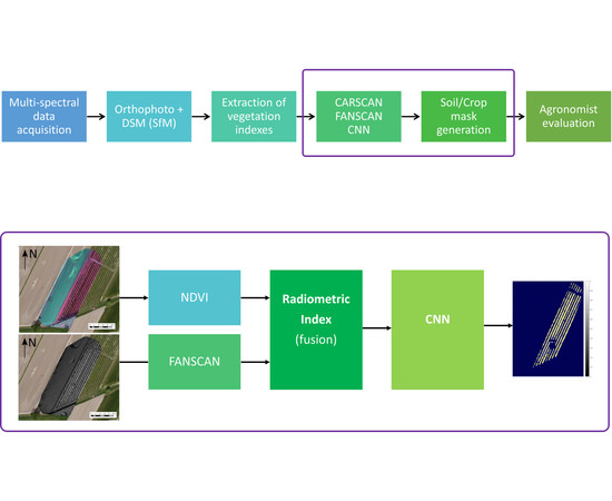
This section introduces different methodologies developed to segment soil and crop from remotely sensed data. The presented methodologies start from a multi-spectral orthophoto and derived DSM. Figure 1 depicts the workflow behind this research, which broadly reflects that common to precision agriculture scenarios. Specifically, precision agriculture requires data to make decisions to improve yield, reduce the rate of fertilizers/pesticides as the number of operations. The remotely sensed data, as presented here, help the agronomist to evaluate the different nutritional plant stresses, such as nitrogen/water, in order to generate prescription maps that can be used by variable rate controllers on tractors to differentiate operations in a given field. The use of remotely sensed data is therefore a useful part of a larger puzzle involving historical data such as soil maps, yield maps and, last but not least, satellite data.
2.1. One Dimensional Rasterization
The DSM is the output of an orthorectification engine that processes high-resolution images (with a typical ground sampling distance (GSD) in the 10–50 cm range). The overall orthophoto DSM image is the algebraic sum of the soil (symbol ) and object (symbol ) fields:
The combined terrain and foliage signal y is raster scanned along a coordinate direction such as z. Separating out the original surface h into a series of sample points in the z-direction obtains a set of ‘unrelated’ one dimensional images ready to be processed independently.
Taking an arbitrary section across the image in Figure 2 can reduce the problem of soil extraction into a series of one-dimensional sub-problems that are theoretically easier and faster to process. Therefore, at some fixed z:
where and are, respectively, the tree and soil fields across some given z-coordinate.
The function y, when discretized, is never in , the set of all one-fold differentiable functions. Differential methods are not general enough without significant pre-processing and a potential loss of data. Fourier transforms are unsuitable due to the instability of the FFT when the signal is contaminated with any significant level of noise: any potential advantage that a low pass filter would have is negated by the fact that any attempt to control noise through expedients, such as Weiner or spectral filters, will tend to remove high frequency details from the image. In this way the quickly-varying tree or contoured terrain signals are inaccurate or even omitted completely. We will show below that the use of a direct method can recover information from the Fourier space in a non-destructive fashion.
The digital nature of the data allows the use of efficient filter sets designed to separate a slow digital derivative from a relatively fast one. We will show below that this observation can be linked to statistical integral methods for solving the general problem.
Trees on the ground can be defined by their scatter probability density function . The importance of this function is in defining the nearest neighbor distance from any given point . Idealizing, at some point, the tree population probability density function maximizes locally over some differential . The associated probability density maximum is therefore constrained over some nearest neighbor contour on the -plane:
The nearest neighbor (generally non-differentiable) probability contour serves to define a correlation distance or integral of a tree or other object class to its nearest neighbors. Every point on the nearest neighbor contour will tend to satisfy a maximum of this correlation integral:
In one dimensional language this equation simplifies to:
over the object separation w. In other words, when this integral is at a stationary maximum, it corresponds to a local probability maximum in one dimension that dictates the local distance w to a nearest neighbor for the object class . The local spatial frequency of the object class at the point x is:
and corresponds to the Fourier or correlation frequency of the object class embedded into the signal y. The frequency distribution of object classes on the ground gives rise to a relative symmetry: when the solution of Equation (3) is a correlation minimum, from Equation (2), the cross-correlation function of the soil will be a maximum instead:
At such points y is a local minimum since there is no object field, by replacing with a normalized window k of integration width w:
for some constant c. If the integration window width is made equal to the correlation distance less the object width b in the field at x then the inequality is removed on the left and we have:
for any point x that is inside the window of integration but outside the object . Applying a spline operator S to the set of all points
smooths the soil field data to a resolution of :
where inf represents the greatest lower bound. From Equation (2)
In practice, the dimension b of a local object is not essential knowledge if one manipulates Equation (7) into:
where the integral is taken over the range with and . The resulting set of points are solutions to Equation (5) and are exactly where the correlation integral (4) of the object class minimizes.
2.2. Derivation of the DSM/NDVI Index
A neural network strongly depends on how it has been trained and what it has been trained on. For this reason, neither of the two approaches, deterministic feature extraction nor deep learning feature extraction, can be described as completely satisfactory for the intelligent processing of UAV data, and much of the literature reflects this fact. However, as remarked so far, the next logical step is to assume that both a supervised learning approach and a deterministic methodology (e.g., [21]) such as the one presented here may improve the state-of-the-art at low training energy. For example, by introducing natural information that removes the need for artificial thresholding and other parametrization that can be resolved naturally within the framework of the data itself. One good way of achieving such data representation is to fuse together the output signal from different instruments or different transformations of the data.
We found that the key to doing this is to recognize that the information contained in the DSM object field and the NDVI index have mutually exclusive relationships to potentially relevant image pollutants. This is what can be efficiently filtered using basic set theoretical methods and only then sent to a neural network for a pattern recognition analysis. This, as opposed to a complicated neural network that operates on the basis of an independent index or other segmentations, which, in our opinion, is expensive and unreliable to try to achieve in terms of agricultural training data on the remote sensing scale. In particular, such an approach has more in common with brute force methodologies than a general optimization of the best qualities of each available data source and processor—creating an unreliable system overall.
For generality, consider a deterministic Hough, K-means or DSM object field segmentation of a terrain with canopy, buildings and cars included in the image characteristic pixel set D (see Equation (17)). Consider also a radiometrically indexed image pixel set R of the same terrain, with both grass and canopy features in high probability pixel positions. The precision agricultural information of greatest value is the canopy image set C that, in terms of Baye’s probabilities P, can be defined at the pixel level through the set theoretic relation:
for a given field at a given time under a set of given environmental conditions. This is our model for tentatively combining the two approaches in a DSM/radiometric preprocessing stage for a neural network. This neural network is not configured to segment extensively, as is currently the trend, but rather to differentiate the DSM/radiometric filter and obtain the plant canopy probability tiles from it. The convolutional neural network effectively performs a geometric pattern recognition on high resolution image data to detect the presence of a vegetation canopy against ground truth training data. This is also in line with the interpretations put forward in Equation (3).
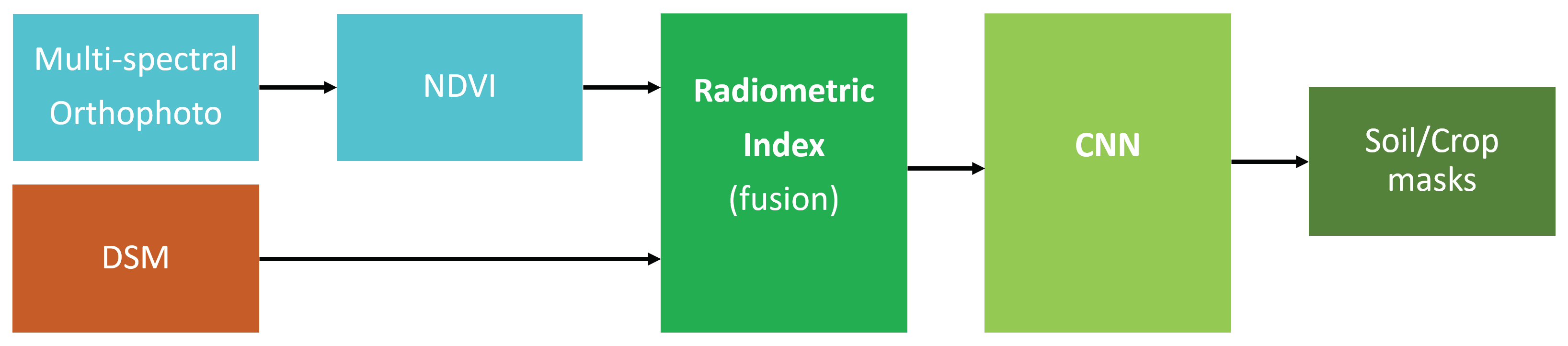
If that is true then we propose the probabilistic DSM/NDVI radiometric index for remote sensing images using Equation (14):
The structure of this equation is interesting: the NDVI signal is now thresholded by the natural ground based features found in the DSM object field. The radiometric absorption image probabilities are now modulated in a natural way by the DSM probability interpretation made in Equation (3) in Section 2.1. However, the relationship is mathematically symmetric: the radiometric measure also modulates the DSM object probabilities to produce a fused DSM/NDVI data stream that contains the relevant information from both, but clears the improbable feature sets that each of them is able to acquire as part of its natural physical characteristics. Figure 3 depicts the adopted strategy to combine and use DSM/radiometric data.
2.3. Control Dataset
2.3.1. Noise Benchmarking Dataset
To benchmark the operation of these mathematical results over the DSM plane when noise is present, we generate a unit white noise signal over a constant height crop DSM arbitrary units overlaid onto a Gaussian hill profile, :
The white noise taken together with the crop simulates an erratic object set of average height 2.5 units and standard deviation 1 arbitrary unit over the soil (see Figure 2). The maximum height of the object field is therefore about 33% of the maximum height of the hill (∼15 units) and will have a non zero derivative. As will be shown below, this fact allows Equation (13) to segment out the rapidly varying quantity from the smooth terrain below it.
2.3.2. Real Flight Dataset
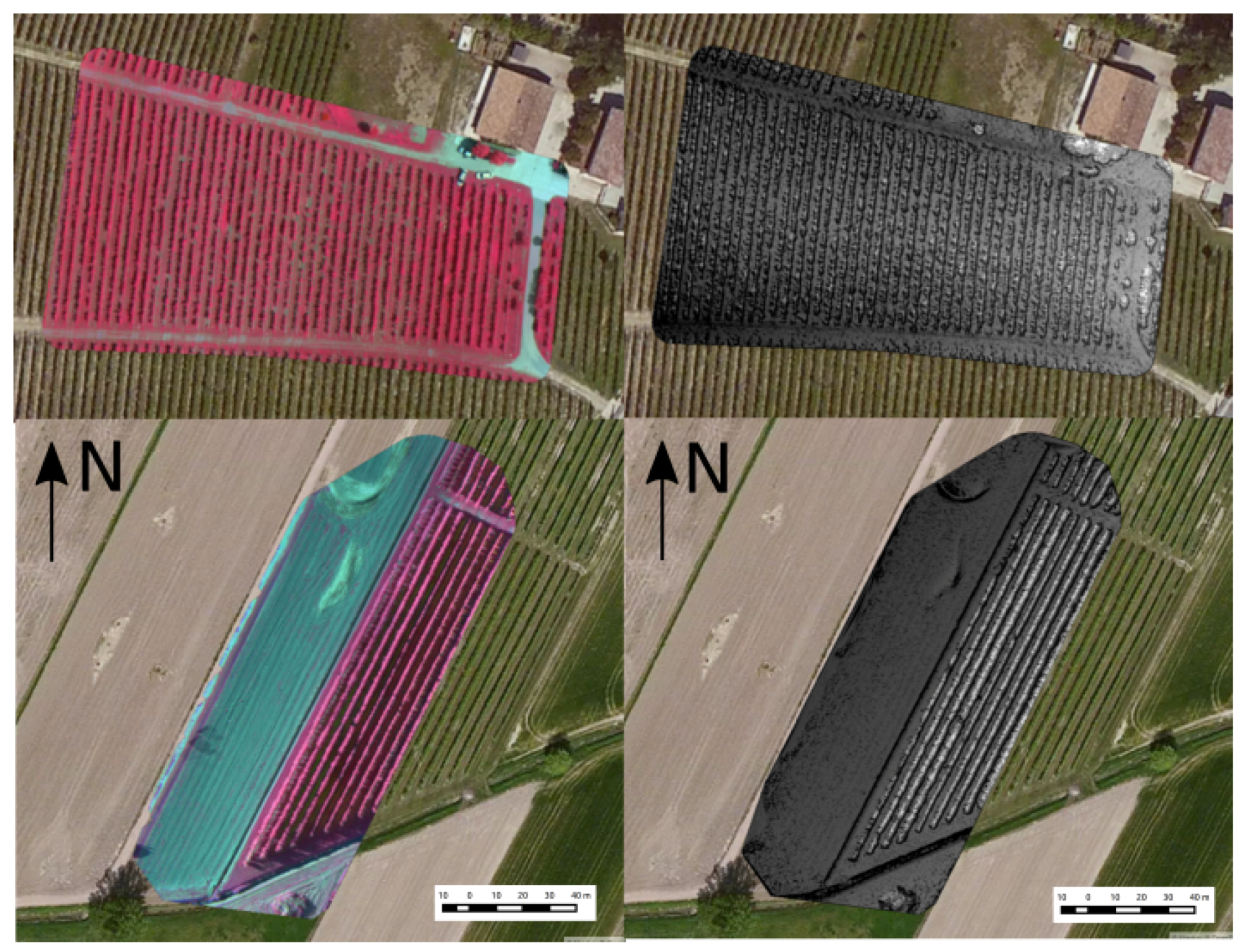
To test the methodology on real data we, obtained multi-spectral data from UAV flights over a hilly farmland area. The acquisition campaigns were performed with an AscTec Pelican equipped with the Sequoia multi-spectral camera. Figure 4 shows the study areas and the extracted DSM. The final orthophotos have a final GSD of 4 cm with ±0.5 m of horizontal accuracy.
The quality of acquired data reflects on both orthophoto and DSM. Quality is mainly influenced by the attitude of vehicle during the acquisition, height above the ground. This last aspect plays a key role especially in hilly areas. If the mission was planned with a constant height then each single image will have a different GSD especially in areas where the underlying soil gradient is high. Therefore, we tried to set-up the experiment by using a constant height above the ground even if this required an a priori knowledge of the DEM of the area.
Study area 1 represents a hilly area of vineyards where several rows of trees are present with varying spatial frequencies. Trees have an average height above the ground of 2 m with a small canopy at the top (0.7 m). Study area 2 represents an area covered by fruit plants with a small and constant slope over the area.
3. Results, Algorithms and Verification
3.1. Work with the CARSCAN Algorithm
CARSCAN is a DSM that uses a Cartesian grid generalization of Equation (13) over the terrain image. The noise benchmarking dataset (see Section 2.3.1) of the Gaussian hill (see Equation (16) and Figure 2) is tested through the basic CARSCAN algorithm over the artificial terrain model in the dataset. It aims to segment both the artificial white noise and object fields from the hill profile (see Figure 6) and in so doing demonstrates that Equation (13) is indeed a robust foundation for segmentation algorithms.
3.2. Work with the FANSCAN Algorithm
FANSCAN is a radial grid rasterisation DSM which, as we will see, does indeed recover more information from the original image on the Fourier plane. To see how it does this in detail, we use the Real Flight Dataset (see Section 2.3.2) for both study areas taken by aerial survey (noise included, see Figure 4) to test CARSCAN against the FANSCAN algorithm. As expected, this leads to a demonstration of the mathematical properties of the algorithm in Fourier space. Finally, the object field DSM derived from FANSCAN will be polluted with a common artifact and fed together with the DSM/NDVI index (calculated from Equation (14)) into a simple pattern recognition CNN to derive the required recognition of crop in the field.
3.3. CARSCAN: Cartesian Grid Soil Field Extraction
Repeated raster scanning of the field along the z axis generates an array of vectors along x. Each vector in this array can be operated on with Equation (13) to develop the soil profile at some value of z as a function of x. Used in this way on the entire profile array, Equation (13) will generate a surface soil field at some integration window width w (see Equation (13)). Here, instead of applying the spline operator S to the one dimensional Equation (9), it is faster and more expedient from a computational point of view to apply a grid interpolation operator G (written in c++ and accessed via Python’s Numpy framework for example) to the soil surface data, . Algorithm 1 codifies this methodology.
| Algorithm 1 Pseudo code description of a Cartesian soil field extraction. Input = discretized horizontal image slices . Output = and fields. |
|
To test the DSM object and noise field extraction properties for CARSCAN, we now use the noise benchmarking dataset (see Section 2.3.1). The objective is to take the complete polluted profile (see Figure 2) and to pull out the DSM for the Gaussian hill, .
The field that results from Algorithm 1 is the original Gaussian hill profile. This two dimensional functional representation of the soil signal is then used to extract the variation over just the terrain using Equation (1) directly, resulting in the object field (see Figure 5).
Defining the characteristic function of the signal:
allows a quick graphical appreciation of the object detection/classification area in the DSM model. This is correctly calculated in Figure 5, where the threshold level is set to the mean object field height.
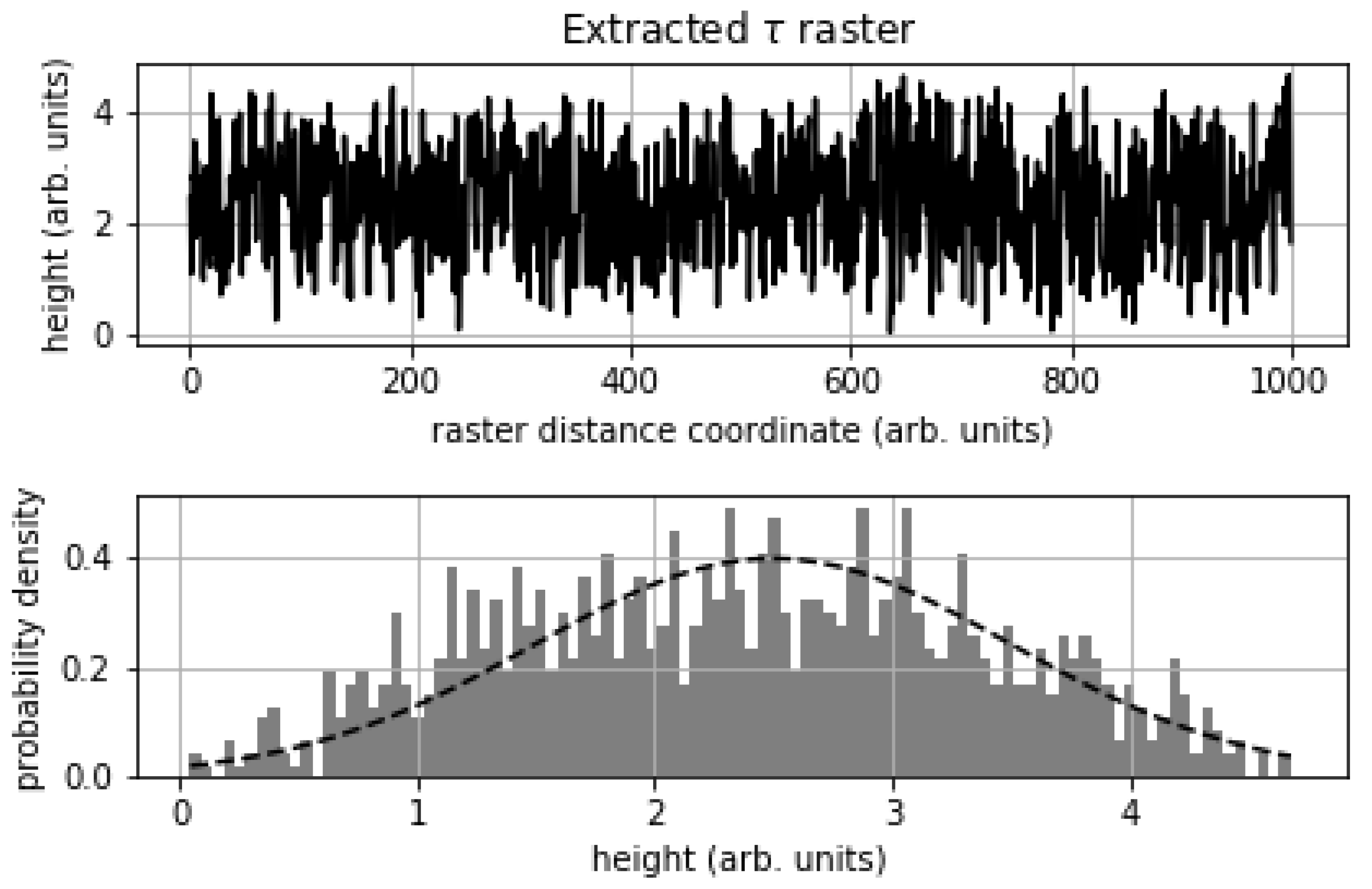
Figure 6 shows in detail the performance characteristics of CARSCAN during the Gaussian hill profile test. The time series extracted from Figure 5 (image pixel coordinates, principle diagonal) shows a completely stochastic trend over 1.000 samples taken along the line of integration. The probability distribution of the time series shows a clear similarity to the original (dotted line in the lower graph shown in Figure 6) generating density function. This behavior is entirely expected and is due to the integral nature of the filter (Equation (13)), Algorithm 1 is therefore quite noise resistant, tending to preserve or segment noise into the object field (up to the maximum tree height) and thus removing it from the soil field.
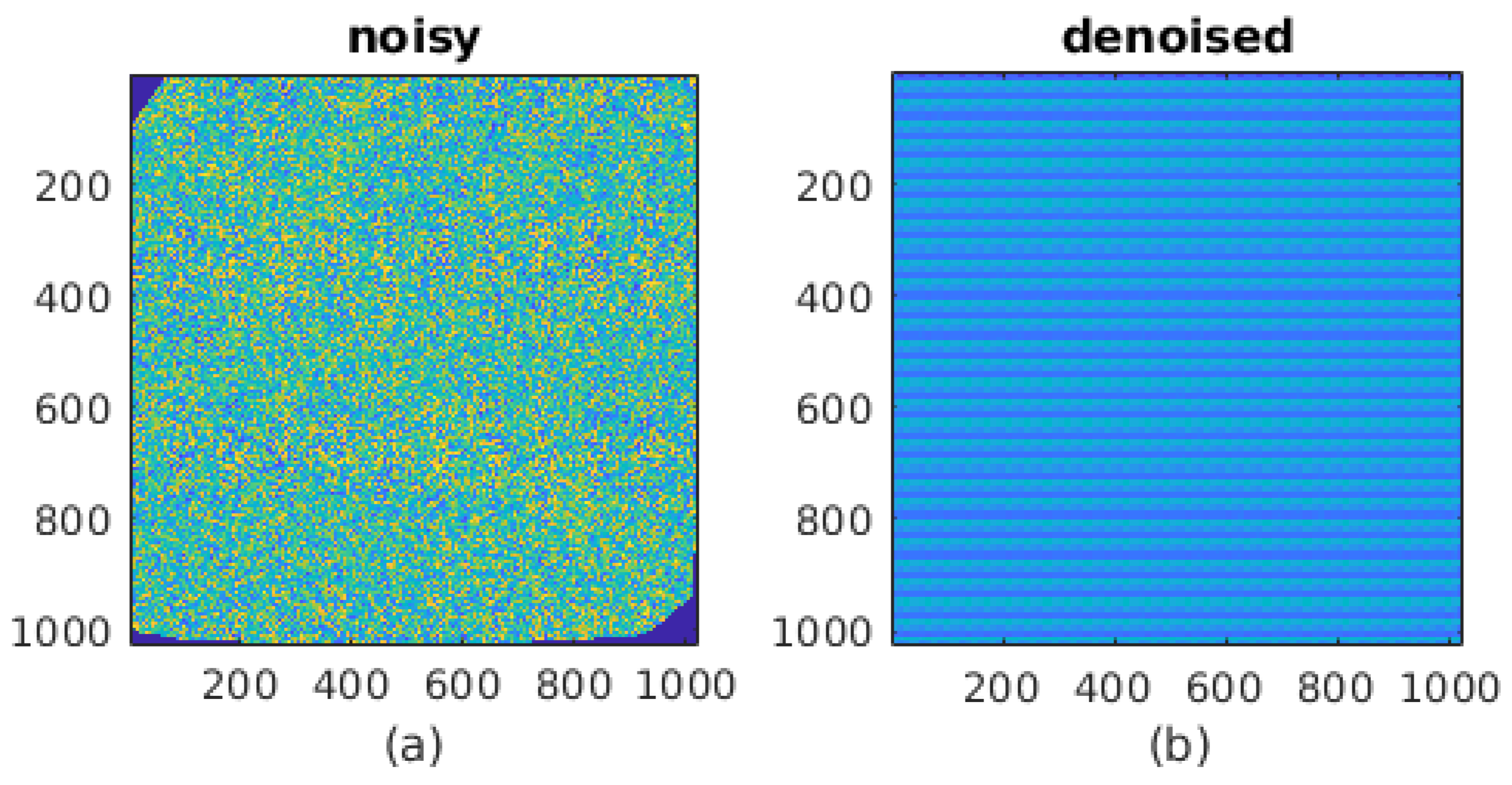
The Burger MLP [22] provides an ideal denoising platform for the CARSCAN output. The image derived from Figure 2 is fed directly into the MLP, resulting in a denoised image of the terrain as shown in false color in Figure 7.
To compare the quality of the recovered crop signal by the algorithm/MLP combination we recourse to Table 1, which confirms the visual impressions in Figure 7 that the MLP succeeds in smoothing out the noise, but at the same time reduces the image intensity. The Peak Signal-to-Noise Ratio (PSNR) calculation in Table 1 against the ground truth confirms this immediately—the denoised image shows a degraded PSNR. The PSNR of the ground truth to the noisy image is 7.21 dB. This falls to a value of 5.28 dB, which if taken by itself indicates a noisier image. This power anomaly can be corrected by equalizing the brightness of the denoised image with respect to that of the noisy image and the corrected values are also reported in the table below. This time, the denoised image has a PSNR double that of the noisy image. Corrected this way the PSNR is sensitive to changes in the standard deviation of the noise as opposed to shifts in image brightness.
3.4. FANSCAN: Moving Radial Soil Field Extraction
The rasterization method provides a convenient recipe for separating the aerial image into object and soil fields, as was demonstrated by the CARSCAN algorithm above. This Cartesian strategy can be envisaged along any direction in the image to yield information particular to that orientation. The advantage of such rasterized vectorization (or radial scanning) of the image is that it produces more information about the image frequencies in an off-axis direction and is therefore akin to a high resolution Fourier sampling of the ground object frequencies along some line L. The essential difference is that this is a direct space and hence more stable methodology for sampling complex terrains, with the advantage that the numerical errors commonly associated with passages into and out of transform spaces can be avoided while collecting information on those frequencies. An algorithm designed around this principle would in theory be capable of obtaining the most complete directional frequency scan of an image in direct space. It would also be expensive to compute.
One way of getting this design to work is to make the series of direct horizontal rasters across the image in the CARSCAN algorithm act as seeds for such a strategy. A given raster at can be rotated along any direction in the image and rasterized to develop a one dimensional picture of the object distribution along that line. Equation (17) would then develop the object and soil extractions for the raster as planned earlier but in the direction . Fanning the original raster along all the possible directions forms a basis for the FANSCAN algorithm presented here (see Algorithm 2 and Figure 8).
| Algorithm 2 Pseudo code description of FANSCAN. Input = discretized radial image slices . Output = raw raster point field. | |||
| 1: | procedureFANSCAN(image,slices) | ||
| 2: | |||
| 3: | |||
| 4: | ▹ | ||
| 5: | vertical scan ath: | ||
| 6: | for do | ||
| 7: | ▹ | ||
| 8: | raster scan at θ: | ||
| 9: | for do | ||
| 10: | |||
| 11: | |||
| 12: | for do | ||
| 13: | |||
| 14: | end for | ||
| 15: | end for | ||
| 16: | end for | ||
| 17: | end procedure | ||
FANSCAN delivers the soil and tree segmentation as a series of degenerate raw data points classified along their raster directions through the fan or direction vector (we take this symbol to mean both a direction or discretisation set of vectors as will be apparent from the context). Equation (13) applied along any of these directions extracts the soil component of the raster and can be used to develop a directionally sensitive picture of the soil structure at any point in the image. The data that contains this information is a three dimensional point cloud that is interpolated to fit the original point cloud of the raw image to extract a directionally rich soil field DSM model .
To test the DSM object and noise field extraction properties for FANSCAN, we now use the real flight dataset (see Section 2.3.2). The objective is to take the aerial images (see Figure 4) and to pull out the DSM, , for each one.
Once the DSM soil field has been extracted from the FANSCAN algorithm in this way, the original image and it can be subtracted over the plane to extract the three dimensional point cloud, which is in fact a high resolution DSM object field of the image in direct space.
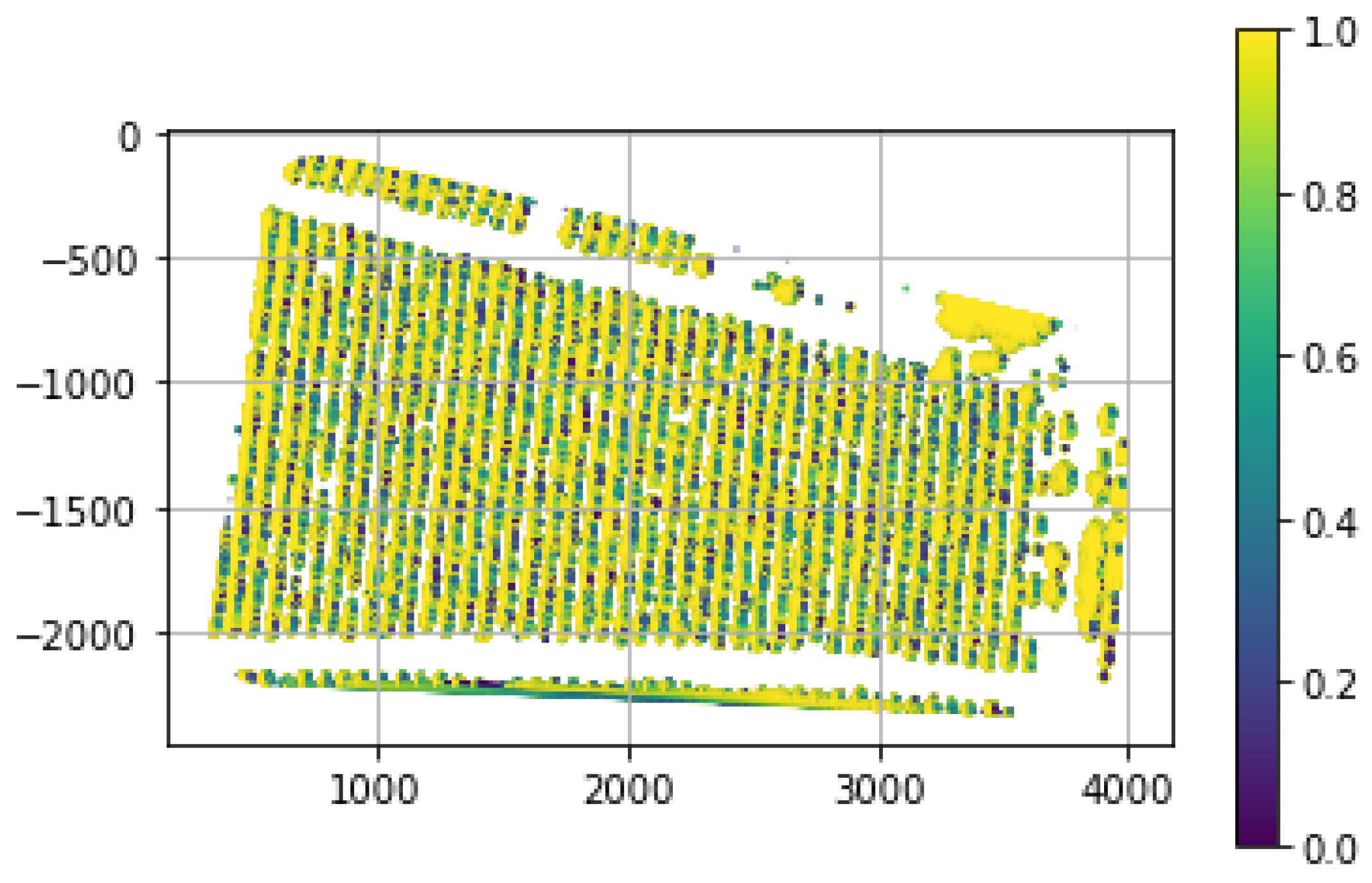
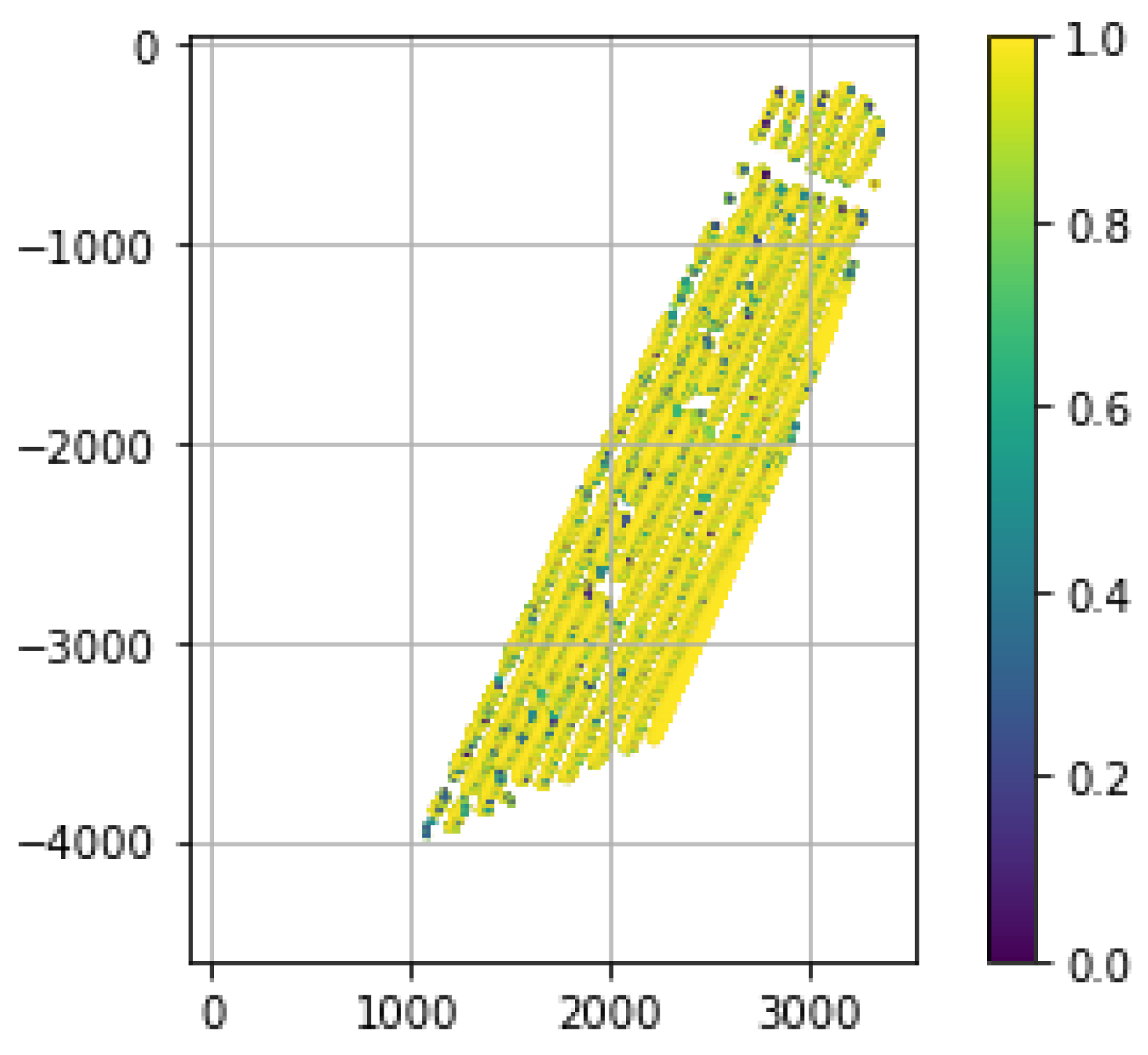
Using the top right DSM in Figure 4 and applying Algorithm 2 obtains the interpolated object field characteristic , as shown in Figure 9. The same procedure is applied to the bottom right DSM in Figure 4 and obtains the interpolated object field characteristic , as shown in Figure 10. The extraction metric for these images are the left and right graphs in Figure 11.
3.5. Convergence Properties for FANSCAN
If we ignore numerical sources of error, the fact that Equation (13) is bounded means that increasing the image discretisation produces a Cauchy sequence of images tending to the “true” soil field image. Since the benefit of using a radial scan in this manner is to provide more information on directional object features, a metric defined in Fourier space will be connected to the object frequencies in Equation (6). To compare the CARSCAN and FANSCAN algorithms, we start with the basic mathematical properties of FANSCAN and use them to work out the mathematical distance from a CARSCAN evaluation of the soil field for the same number of horizontal seeds.
Ideally, the “convergence” of a FANSCAN extracted image can be written as:
where is the fast Fourier transform of the true underlying soil field image, , and is the computed fast Fourier transform of the interpolated approximation, , to it. This is just the “percentage distance” the FANSCAN algorithm has “walked” towards the “true” value of image , written here as . Equation (18), as it stands, is impossible to calculate because in this case the true soil surface is of course unknown. However, there is a classic way around that problem if we invoke the Cauchy convergence criterion for some sufficiently large i:
Then:
Now we can redefine Equation (18) by using the fact that adjacent products of Equation (19) cancel:
where is the “percentage similarity” between the initial and final resolutions of the approximated image. As seen in Section 3.4, if FANSCAN is stopped at then, by definition, the result is a CARSCAN procedure. This is just FANSCAN at fanning vectors. Thus, as was seen above, the CARSCAN image is the “zero order” approximation to any higher order FANSCAN applied across the DSM orthophoto. Specifically, fanning vectors produces a FANSCAN image of resolution proportional to . In this sense the distance between the CARSCAN and FANSCAN images is defined:
It will be observed that under these conditions, Equations (20) and (21) imply that:
which defines when the algorithm has converged.
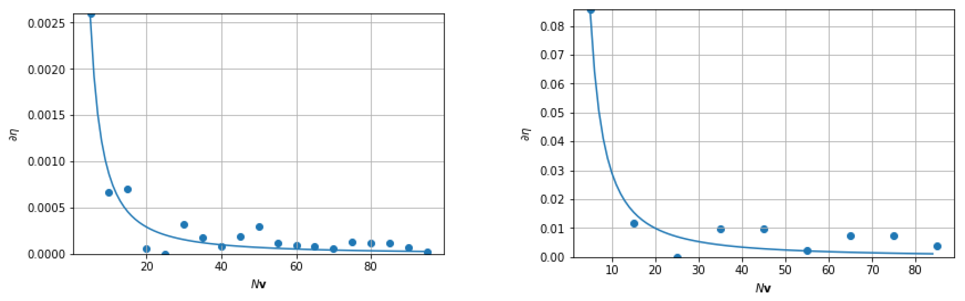
In a world where numerical round off and image noise are significant technological issues, Equations (20), (22) and (23) can be interpreted to say that when the FANSCAN algorithm has converged to its best possible image value, the distance of that image to the equivalent CARSCAN result is maximized and stable for further iterations. In simpler terms, one cannot do better than Equation (23) using just FANSCAN. Therefore, when is at its least possible value the “quality” of the FANSCAN DSM segmentation is maximal. The results of Equation (23) are calculated for the DSM data shown in top right and bottom right images of Figure 4 and plotted in Figure 11.
3.6. Convolutional Neural Network: A DSM/NDVI Strategy
All calculations carried out for this research were done on an Intel® Core™ i7 6820HK Processor with 32 Gb DDR4 2133 MHz SDRAM and a NVIDIA® GeForce® GTX980M GPU with 4GB GDDR5. The programming platform was Python 2.7 and some trials were carried out on MATLAB®.
In what follows, we develop an example using a simple supervised CNN to test how effective the strategy presented in Section 2.2 can be when using a DSM/NDVI index. The baseline is set to be the performance of the network in discerning crops using only NDVI, only DSM and then with the DSM/NDVI index defined by Equation (15). The CNN we used for these experiments was a standard image object detection framework, which uses a convolutional neural network to classify 28 × 28 square pixel image tiles within a larger image.
The network training follows the transfer learning work flow that is commonly used in deep learning applications [23]. The network is trained on a large collection of images [24], and then used to solve a new classification or detection task. The advantage of transfer learning is that the number of specific images required for training and the training time are reduced. The present CNN is initially trained using the CIFAR-10 data set, which has 50,000 training images. Then this pre-trained CNN is transfer trained for crop object pattern detection using just 90 training images that have been segmented for aerial views of crop patterns at the dimension scale of the orthophoto (see Figure 12).
The training sets were constructed directly from samples taken from the output of the DSM segmented images. The object field was sourced from the FANSCAN algorithm, for example the training set element in Figure 12 is taken from the DSM object field in Figure 17. That is to say, height and random border variation on the object field is what the CNN was trained to search for when it had to classify a plant, while black pixels it associated by default with soil (see the discussion following Equation (15)). Should anything fall in between these two images—it is classified as ‘other’, which may be cars, buildings or other man-made structures included in the DSM object field segmentation. This training scheme therefore tends to reflect the natural information hierarchy encoded inside the DSM/NDVI map—black for automatically thresholded soil (since it has been segmented out by Equation (13) and represents a zero information state in the DSM object field) and plants when for high probability NDVI and DSM patterns. This amounts to the DSM modulating the mathematical amplitude of the NDVI signal and vice-versa, and the consequence of this mathematics is that the CNN is trained to perform a specialized crop edge detection along rows of crops. When a crop edge is located the CNN identifies it as a high probability (>70%) yellow colored tile and when it is not, tile is colored as a blue square (see Figure 15).
To increase training efficiency we also used an image augmentation technique which included randomized scaling, rotation and translations of the training data to increase the network’s robustness or invariance to these affine transformations on the plane. The fact that the network is over specified in design and limited to just three crossentropyx (i.e., cross entropy function for k mutually exclusive classes) classifications drastically increases the dropout rate and renders the training more efficient. The 90 images were divided into a 75:25 training to validation set ratio as is common practice in deep learning applications.
The network achieves a transferred classification efficiency of 100% by setting up and training mini-batches of the 68 images for over more than 20 epochs, cross validating from the 22 remaining images at the close of every epoch (see Figure 13). Once training has been completed the CNN is ready to differentiate crop from soil or classify the object as ‘other’ (see Table 2 and Figure 13).
In order to test Equation (14) with this pattern recognition CNN, we use the (bottom right) DSM dataset in Figure 4 and extract the function already worked out in Figure 10. The NDVI radiometric index derived from the (bottom left) multi-spectral dataset in Figure 4 is shown (left) in Figure 14. Immediately obvious is that the NDVI index alone includes substantial areas outside the rows of crops.
The next step was to pollute both the NDVI and DSM images with an artifact not present in the ground truth images used to train the CNN (see Table 2). A practical scenario was to place a small building or other man made structures with an adjoining grass area artificially into the crop field so that only a subset of naturally exclusive features would be present in the radiometric and DSM images. In simpler terms, this means that we deliberately add a grass and building anomaly into the test in an attempt to try and confuse the CNN. The modified test images are centre and right in Figure 14 for the NDVI and DSM signals, respectively.
The grass NDVI index was simulated from a Gaussian distribution and the adjoining building or man-made structure is higher than the threshold height used for calculating the DSM picture. For its NDVI index, the man made structure is ranked well below unity and so is absent from the simulated NDVI image completely. However, the grass area is present at a mean index strength of 0.55 with standard deviation 0.225, which is a close match to the ground truth NDVI index of the crops. The geometry of the grass plot is a small square measuring 300 × 300 square pixels. In the DSM, on the other hand, this grass is well below the threshold height and, consequently, completely absent from the DSM image. For its representation on the DSM plane, the building is present at a uniform strength of units and measures 300 × 100 square pixels.
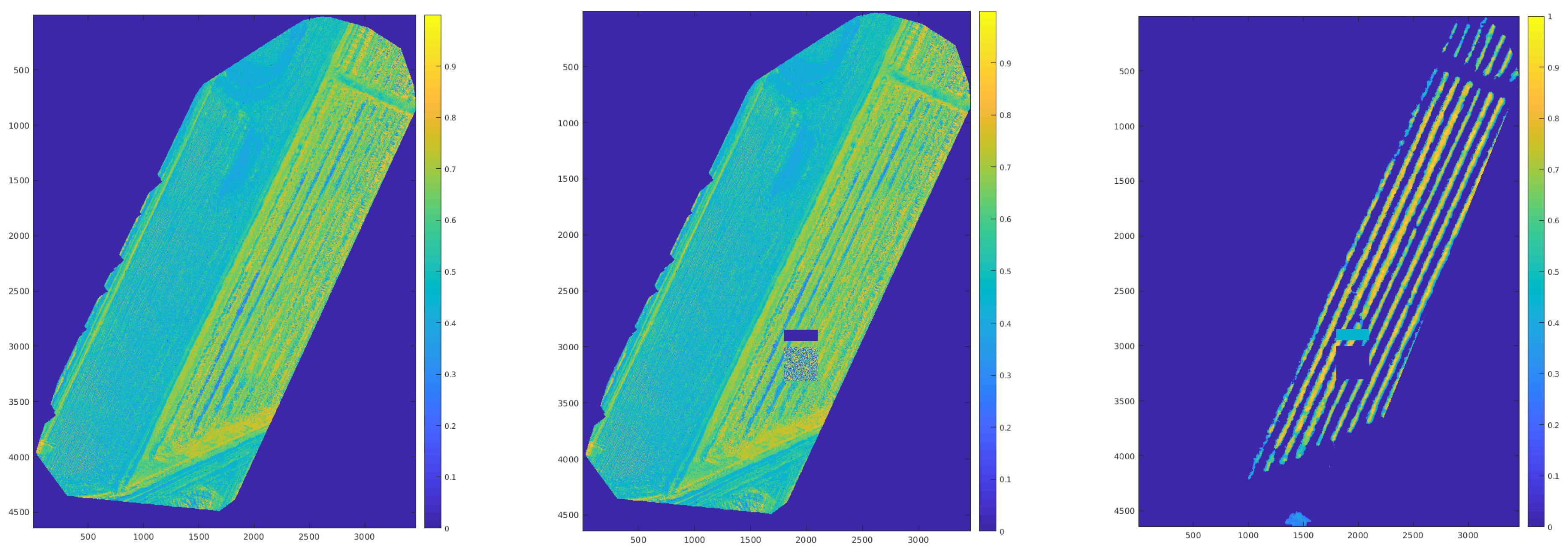
As a first test, the CNN is fed the modified NDVI image by itself and the results are shown left in Figure 15. Crop and grass are indeed identified together including the border areas and substantial parts of shrubbery in on the adjoining field. For the second test we move to pre-filtering the data, fusing both NDVI and DSM data streams using Equation (15) as the model. In this scenario the CNN extracts only groups of pixels (or tiles) with probability of crop presence exceeding 70% and the result is a correct crop extraction (see the centre panel in Figure 15 and Table 3) with no visible artifacts. As the third and final test, the CNN is given only modified the DSM object field and identifies the crops and correctly excludes most of the man-made structure with significant probability indicating that the man made structure is part of the crop (see the right panel in Figure 15). Furthermore, this last test has also included some shrubbery at the lower part of the figure.
Table 3 below summarizes the quality (density) of the DSM/NDVI-CNN tests of Figure 15 in terms of the relative ground truth gain or brightness of every image defined as the ratio of the number of correctly identified (black) 28 × 28 pixel tiles in the man-made structure to the ground truth expectation value for that image:
The ideal value for the gain (or brightness) is 100%. This value signifies that the result of the segmentation is congruent to the ground truth geometry and that all tiles have been correctly identified.
4. Discussion
4.1. Convergence in Fourier Space
Figure 11 demonstrates the convergence properties—and hence the robustness—of the theoretical framework proposed in Section 2.1 and the subsequent implementation of those ideas in Section 3.4. The series of iterations produces a figure sequence of ever increasing detail in frequency space, which is unsurprising. However, the fact that the results for both sets of DSM data, each markedly different from the other, produce very similar convergences is of note. It seems to imply that the FANSCAN procedure does not depend on the precise geometry of the soil or the crop distribution in the photos, but perhaps depends more on the resolution or detail present in them.
The existence of an asymptote in both DSM configurations also implies that the algorithm is capable of extracting frequencies below a theoretical maximum from the photos in direct space, as hoped. This feature is important because it also tends to steadily denoise the object field DSM. We saw in Section 3.3 that the CARSCAN (and by extension FANSCAN) procedure tends to dump high frequency noise from the original DSM image (see Figure 4, right) into the segmented object field DSM (see Figure 6). Taken together with the fact that every iteration in FANSCAN uses the spline operation S in Equation (10) (or its two dimensional equivalent G in Section 3.3) at ever greater levels of directional sampling, the CARSCAN result at is radially averaged for every iteration beyond it. Evidence for this can also be seen in the convergence curves of Figure 11 where the fluctuations in the image derivative decrease with .
The images are steadily computed at higher levels of accuracy until the algorithm cannot extract any more information from the data (appearing as the asymptotes in Figure 11). This limit corresponds to every pixel having been analyzed and averaged over the plane, not unlike a convolution. The resolution limit therefore implies an upper bound to the frequency present in the data on the Fourier plane—the discretization or instrumentation limit.
Thus, moving backwards along the abscissa in Figure 11 and reducing the raster discretization to zero (i.e., towards the CARSCAN rasterization) shows an accompanying depreciation in the Fourier space of the algorithm and an increase in the possible noise content of the extracted object field DSM. Properties such as these can only help to strengthen the performance of potential denoising algorithms (see [22,25]) associated with deep learning applications.
4.2. Radial Raster Geometry: An Achilles Heel
Running FANSCAN on this data shows the theoretical consistency of the method and at the same time an inherent weakness in its geometric design.
When a raster vector falls directly upon a row of trees, the soil extraction as developed in Equation (13) will fail. This aspect is nicely illustrated in Figure 16 for the bottom dataset in Figure 4, where part of the object field gets extracted out with the soil field at around fans.
There are several solutions to this problem and all of them involve avoiding such a situation in the first place. One solution is to limit the maximum resolution (number of FANSCAN raster lines) manually. The second is to randomize both the horizontal seeding and the FANSCAN rasterization. A combination of both of these measures can produce good results for the simple test images, as studied here, but will fail in places for complex object field extractions.
The more costly, but guaranteed solution, is to search successive soil field approximations for competing minima and to reject any outliers from the soil field sequence. There are however considerable difficulties in achieving this: the main one being that the physical number of points in each extracted image is different and therefore extensive use of back interpolation needs to be made to co-register the entire sequence being considered for correction. That can require lots of memory (∼Gigabytes) for even the most modest of images.
While a fully automated solution can take time, in essence all that is actually required is one artifact free image from the sequence so that artifacts in the sequence can be automatically recognized and then removed. Following the discussion above, a good candidate for that image is the very first (CARSCAN) iteration: . Using Hadamard products, the logical matrix operation:
will quickly post process and correct the artifacts from the soil field. The multiplicity of rasters across the object field makes it highly unlikely that the object field is adversely affected by this phenomenon, so no correction need be applied. However, if necessary, it is easily generated together with the soil field correction itself, as shown in Figure 17.
4.3. The DSM/Radiometric Approach to Canopy Segmentation
In Section 3.3 we recovered a test crop signal by using an efficient denoising MLP. In Section 3.4 we demonstrated the development of a high resolution technique (see Algorithm 2) for the object extraction, and possible noise reduction, through increased frequency sampling of the DSM data, presented in Figure 4 of Section 2.3.
Section 2.2 uses the Algorithm 2 (FANSCAN) derived characteristic image together with the NDVI multi-spectral radiometric index from Figure 4 bottom as arguments to Equation (14). This defines a new input to an object recognition CNN transfer trained on 90 images of crop pattern data for evaluation of the NDVI radiometric index. To this end we deliberately weakened the original data by polluting it with a typical man-made structure among the clearly identifiable crop masses, as shown in Figure 14. The NDVI index was then extracted for the polluted image along with its associated artifact ridden DSM object field, ready for testing the DSM extraction technique FANSCAN and Equation (15).
The artifact NDVI signal was fed into the neural network and the results of Figure 15 left showed that, as expected, the CNN failed to segment the grass object field from the ground truth crop canopy, which has been stated to be an important consideration in this article. This observation is reflected by the value of the corresponding poor value of the tile brightness ∼20% in Table 3. This fact indicates that most of the original NDVI vegetation pixels have been—incorrectly—retained by this small and relatively under powered CNN.
Figure 15 right tested just the DSM object field derived in Figure 14 right as an input image for the object recognition CNN to evaluate: although the visual result looks appealing, the brightness value shows that a significant number of tiles fails the >70% probability test. It is also clearly visible that the test fails to segment the whole man-made structure from the crop and that the shrubbery at the bottom of Figure 14 right has been counted into the crop population. The registered gain or brightness for the image is 225%, which is difficult to explain. Theoretically the entire man-made structure is worth only 38 tiles and the network has selected fewer than these—therefore the error originates elsewhere, for example at the borders of the grass plot, where it is plausible that, given the training of the network, another 43 tiles can be expected. In this case, the corrected brightness value becomes 173%, which is not yet sufficient to explain the observed increase. The sensitivity to training is therefore perhaps a clear weakness of the evaluation process, a fact also noted by other authors working on deep learning applications in precision agriculture (see [21,22] for example).
Both these failures can serve to highlight the dangers associated with using either DSM object field or NDVI index data by themselves with a small CNN. This brings into focus the possible importance of a formulation like Equation (14). Figure 15 centre tests the modified Bayesian radiometric filter and it yields a gain or brightness value of 85%—by far the best of the three. In fact it is actually quite close to the ground truth expectation of 100%. While admittedly not perfect, and as yet not sufficiently tested, the DSM/NDVI radiometric index definition does seem to imply and produce in practice a crop identification that is closer to the ground truth than either the DSM object field or the NDVI radiometric index alone. This does to some degree justify our proposal for Equation (15) being a more appealing substitute for a naked radiometric index.
The entire processing pipeline suggested in this article uses simple and stable mathematical building blocks to create a robust and highly automated segmentation pipeline for pattern recognition problems. No parameters were or are required to be set except for the initial training of the CNN and the window width, w in Equation (13) the image dimension. This makes DSM/NDVI appealing as a black box concept. This is not the case for certain unsupervised methodologies [17,18] or indeed specialized convolutional neural networks with high training cost (see [22]). The specially adapted nature of such methods tends to overfit their generic problem types and as a consequence renders them difficult to adjust to different problem scenarios. By contrast, the probabilistic aspect of the theory provides easy extension to an infinite number of data streams through the use of Bayes Theorem and an extension of Equation (15).
It must be noted that the approach of combining data streams is nothing new, see for example [26,27]. It is also important to realize that the DSM extraction strategy, although robust, is costly in terms pre-processing load, which can impede the application of this technique in onboard deployment on real-time analysis platforms such as UAVs (see [28] for a related example). On the other hand, the methodology deployed here is not overtly parametric, and uses a deep learning (generalizable) approach to classify natural probability data. Therefore, it is susceptible to much further development and real time deployment remains for the time being an open question.
Summarizing, after carrying out the proposed benchmark testing, we find that the DSM/NDVI index produces an improvement of about four times compared to its baseline NDVI marker (see Table 3). It does so at practically no extra data collection cost compared to the standard NDVI radiometric index. There is however a reasonable computational penalty for deriving the DSM object field, but this is perhaps compensated to some extent by the fact that the DSM/NDVI measure is nearly as robust as the original NDVI index and has proven to be definitely the best crop/soil segmentation filter in out trials. Furthermore, we also consider the design and quality of the DSM/NDVI-CNN filter as an adaptable methodology with possible future applications in the field of precision agriculture technologies.
5. Conclusions
In this paper we have presented a strategy for integrating terrain height (DSM) images with radiometric index (NDVI) to segment crops and tree objects over soil through the use of high-resolution images from UAVs. The main objectives of our research are:
- increase the automation of the segmentation process,
- make the segmentation of soil from crop using a more robust radiometric index,
- increase the information content of the methodology in a natural way.
The DSM segmentation approach we have devised is based on a nearest neighbor correlation distance technique where the DSM height field is interpreted as a probability density. In this way, Equation (13) demonstrates that a good basis for terrain and tree structure segmentation is possible in terms of simple mathematical analysis. The results further demonstrate that the method potentially enables the correct segmentation of soil and can thus offer insights into the geometric distribution of surface objects upon it.
We have proposed that the Equation (15) image transform be considered as an alternative to the standard NDVI index when used as a data feed into a small image recognition convolutional neural network cross trained to segment object, plant and soil matter. We show that this is indeed a viable proposition that gives a 65% improvement in artifact pixel recognition over the standard NDVI radiometric index.
Future research in this direction will therefore focus upon improving this statistic.
Author Contributions
Data analysis and programming, J.D.; methodology, A.M., J.D., E.F. and P.Z.; writing, J.D. and A.M.; editing, E.F. and P.Z.
Funding
This research received no external funding.
Acknowledgments
The authors would like to thank Carlo Alberto Bozzi of FIELDTRONICS S.r.l. for his valuable support in collecting, developing and analyzing the UAV data during the preparation of this article.
Conflicts of Interest
The authors declare no conflict of interest.
References
- Schenatto, K.; de Souza, E.; Bazzi, C.; Gavioli, A.; Betzek, N.; Beneduzzi, H. Normalization of data for delineating management zones. Comput. Electron. Agric. 2017, 143, 238–248. [Google Scholar] [CrossRef]
- Hedley, C. The role of precision agriculture for improved nutrient management on farms. J. Sci. Food Agric. 2015, 95, 12–19. [Google Scholar] [CrossRef] [PubMed]
- Jin, Z.; Prasad, R.; Shriver, J.; Zhuang, Q. Crop model- and satellite imagery-based recommendation tool for variable rate N fertilizer application for the US Corn system. Precis. Agric. 2017, 18, 779–800. [Google Scholar] [CrossRef]
- Fuentes-Pacheco, J.; Torres-Olivares, J.; Roman-Rangel, E.; Cervantes, S.; Juarez-Lopez, P.; Hermosillo-Valadez, J.; Rendón-Mancha, J.M. Fig Plant Segmentation from Aerial Images Using a Deep Convolutional Encoder-Decoder Network. Remote Sens. 2019, 11, 1157. [Google Scholar] [CrossRef]
- Sa, I.; Popović, M.; Khanna, R.; Chen, Z.; Lottes, P.; Liebisch, F.; Nieto, J.; Stachniss, C.; Walter, A.; Siegwart, R. WeedMap: A Large-Scale Semantic Weed Mapping Framework Using Aerial Multispectral Imaging and Deep Neural Network for Precision Farming. Remote Sens. 2018, 10, 1423. [Google Scholar] [CrossRef]
- Sakamoto, T.; Gitelson, A.; Nguy-Robertson, A.; Arkebauer, T.; Wardlow, B.; Suyker, A.; Verma, S.; Shibayama, M. An alternative method using digital cameras for continuous monitoring of crop status. Agric. For. Meteorol. 2012, 154–155, 113–126. [Google Scholar] [CrossRef]
- Meyer, G.E. Machine vision identification of plants. In Recent Trends for Enhancing the Diversity and Quality of Soybean Products; InTech: London, UK, 2011. [Google Scholar]
- Onyango, C.M.; Marchant, J.A. Physics-based colour image segmentation for scenes containing vegetation and soil. Image Vis. Comput. 2001, 19, 523–538. [Google Scholar] [CrossRef]
- Sogaard, H. Weed Classification by Active Shape Models. Biosyst. Eng. 2005, 91, 271–281. [Google Scholar] [CrossRef]
- Abbasgholipour, M.; Omid, M.; Keyhani, A.; Mohtasebi, S. Color image segmentation with genetic algorithm in a raisin sorting system based on machine vision in variable conditions. Expert Syst. Appl. 2011, 38, 3671–3678. [Google Scholar] [CrossRef]
- Omid, M.; Khojastehnazhand, M.; Tabatabaeefar, A. Estimating volume and mass of citrus fruits by image processing technique. J. Food Eng. 2010, 100, 315–321. [Google Scholar] [CrossRef]
- Omid, M.; Ghojabeige, F.; Delshad, M.; Ahmadi, H. Energy use pattern and benchmarking of selected greenhouses in Iran using data envelopment analysis. Energy Convers. Manag. 2011, 52, 153–162. [Google Scholar] [CrossRef]
- Pang, J.; Bai, Z.Y.; Lai, J.C.; Li, S.K. Automatic segmentation of crop leaf spot disease images by integrating local threshold and seeded region growing. In Proceedings of the 2011 International Conference on Image Analysis and Signal Processing, Hubei, China, 21–23 October 2011; pp. 590–594. [Google Scholar] [CrossRef]
- Pugoy, R.A.D.; Mariano, V.Y. Automated rice leaf disease detection using color image analysis. In Proceedings of the Third International Conference on Digital Image Processing (ICDIP 2011), Chengdu, China, 15–17 April 2011; p. 80090F. [Google Scholar]
- De Benedetto, D.; Castrignanò, A.; Rinaldi, M.; Ruggieri, S.; Santoro, F.; Figorito, B.; Gualano, S.; Diacono, M.; Tamborrino, R. An approach for delineating homogeneous zones by using multi-sensor data. Geoderma 2013, 199, 117–127. [Google Scholar] [CrossRef]
- Yang, C.; Odvody, G.; Fernandez, C.; Landivar, J.; Minzenmayer, R.; Nichols, R. Evaluating unsupervised and supervised image classification methods for mapping cotton root rot. Precis. Agric. 2015, 16, 201–215. [Google Scholar] [CrossRef]
- Delenne, C.; Rabatel, G.; Deshayes, M. An Automatized Frequency Analysis for Vine Plot Detection and Delineation in Remote Sensing. IEEE Geosci. Remote. Sens. Lett. 2008, 5, 341–345. [Google Scholar] [CrossRef] [Green Version]
- Comba, L.; Gay, P.; Primicerio, J.; Ricauda Aimonino, D. Vineyard detection from unmanned aerial systems images. Comput. Electron. Agric. 2015, 114, 78–87. [Google Scholar] [CrossRef]
- Mancini, A.; Frontoni, E.; Zingaretti, P.; Longhi, S. High-resolution mapping of river and estuary areas by using unmanned aerial and surface platforms. In Proceedings of the 2015 International Conference on Unmanned Aircraft Systems, ICUAS 2015, Denver, CO, USA, 9–12 June 2015; pp. 534–542. [Google Scholar] [CrossRef]
- Srivastava, N.; Hinton, G.; Krizhevsky, A.; Sutskever, I.; Salakhutdinov, R. Dropout: A simple way to prevent neural networks from overfitting. J. Mach. Learn. Res. 2014, 15, 1929–1958. [Google Scholar]
- Cereda, S. A Comparison of Different Neural Networks for Agricultural Image Segmentation. MSc. Thesis, Politecnico di Milano, Milano, Italy, 2017. [Google Scholar]
- Burger, H.C.; Schuler, C.J.; Harmeling, S. Image denoising: Can plain neural networks compete with BM3D? In Proceedings of the 2012 IEEE Conference on Computer Vision and Pattern Recognition, Providence, RI, USA, 16–21 June 2012; pp. 2392–2399. [Google Scholar] [CrossRef]
- Girshick, R.; Donahue, J.; Darrell, T.; Malik, J. Rich feature hierarchies for accurate object detection and semantic segmentation. In Proceedings of the IEEE Conference on Computer Vision and Pattern Recognition, Washington, DC, USA, 23–28 June 2014; pp. 580–587. [Google Scholar]
- Deng, J.; Dong, W.; Socher, R.; Li, L.J.; Li, K.; Fei-Fei, L. Imagenet: A large-scale hierarchical image database. In Proceedings of the CVPR 2009. IEEE Conference on Computer Vision and Pattern Recognition, Miami, FL, USA, 20–25 June 2009; pp. 248–255. [Google Scholar]
- Dabov, K.; Foi, A.; Katkovnik, V.; Egiazarian, K. Image Denoising by Sparse 3-D Transform-Domain Collaborative Filtering. IEEE Trans. Image Process. 2007, 16, 2080–2095. [Google Scholar] [CrossRef] [PubMed]
- Sturari, M.; Frontoni, E.; Pierdicca, R.; Mancini, A.; Malinverni, E.S.; Tassetti, A.N.; Zingaretti, P. Integrating elevation data and multispectral high-resolution images for an improved hybrid Land Use/Land Cover mapping. Eur. J. Remote Sens. 2017, 50, 1–17. [Google Scholar] [CrossRef]
- Bittner, K.; Körner, M.; Fraundorfer, F.; Reinartz, P. Multi-Task cGAN for Simultaneous Spaceborne DSM Refinement and Roof-Type Classification. Remote Sens. 2019, 11, 1262. [Google Scholar] [CrossRef]
- Milioto, A.; Lottes, P.; Stachniss, C. Real-time Semantic Segmentation of Crop and Weed for Precision Agriculture Robots Leveraging Background Knowledge in CNNs. In Proceedings of the 2018 IEEE International Conference on Robotics and Automation (ICRA), Brisbane, QLD, Australia, 21–25 May 2018. [Google Scholar]
Figure 1.
Workflow to process multi-spectral images; crop/soil segmentation enables the generation of masks that will be considered by the agronomist to exclude areas out of interest.
Figure 1.
Workflow to process multi-spectral images; crop/soil segmentation enables the generation of masks that will be considered by the agronomist to exclude areas out of interest.

Figure 2.
Gaussian test image of about 1000 × 1000 pixels generated artificially with a rapidly varying stochastic object field over the z-x pixel plane. The y height field is in arbitrary test units.
Figure 2.
Gaussian test image of about 1000 × 1000 pixels generated artificially with a rapidly varying stochastic object field over the z-x pixel plane. The y height field is in arbitrary test units.

Figure 3.
Adopted workflow to combine DSM and multi-spectral orthophoto to feed CNN.

Figure 4.
(top left) Study area 1, derived orthophoto of vineyard area with false color. (top right) Derived DSM (black represents low height) of about 4000 × 2500 pixels. (bottom left) Study area 2, derived orthophoto of plant fruit area with false color. (bottom right) Derived DSM (black represents low height) of about 3500 × 4500 pixels. The scale bar represents 40 m along level ground.

Figure 5.
The result of applying thresholding to at the mean object field height is the membership function . The raster integration line shown in dashed red is the basis for the analysis of Figure 6.
Figure 5.
The result of applying thresholding to at the mean object field height is the membership function . The raster integration line shown in dashed red is the basis for the analysis of Figure 6.

Figure 6.
The DSM noise-object field and its extraction from the original Gaussian hill profile terrain data along the principle diagonal (image pixel coordinates). The true probability density function of the signal is shown in dashed black. The recovered object field is therefore mapped back to a noise signal normally distributed about the mean object field height. Around 99% of the probability mass is successfully segmented in this test.

Figure 7.
(a) The CARSCAN extracted terrain field from the original Gaussian hill profile data as in Figure 5. (b) The subsequent denoising of (a) using the Burger multilayer perceptron (MLP) [22].

Figure 8.
Geometry of the FANSCAN algorithm (see Algorithm 2). The white arrows are the raster vectors across an extracted object field DSM. The dotted horizontal line is the current vertical scan position. Negative pixels on the z axis are an artifact of matrix to image reflection. The vertical color bar is in metres.

Figure 9.
The FANSCAN object characteristic applied to the (top right) DSM data in Figure 4 at fan rasters per horizontal seed point. The color scale is in meters and negative pixel numbers are an artifact of the image to matrix conversion.
Figure 9.
The FANSCAN object characteristic applied to the (top right) DSM data in Figure 4 at fan rasters per horizontal seed point. The color scale is in meters and negative pixel numbers are an artifact of the image to matrix conversion.

Figure 10.
The FANSCAN object characteristic applied to the (bottom right) DSM data in Figure 4 at fan rasters per horizontal seed point. The color scale is in meters and negative pixel numbers are an artifact of the image to matrix conversion.
Figure 10.
The FANSCAN object characteristic applied to the (bottom right) DSM data in Figure 4 at fan rasters per horizontal seed point. The color scale is in meters and negative pixel numbers are an artifact of the image to matrix conversion.

Figure 11.
(left) Absolute value of Equation (23) for the (top right) DSM data in Figure 4: the closer is to zero, the better the quality (convergence) of the image. The solid blue line is a power law nonlinear regression for the measured data and shows the likely value of the quality metric as a continuous function of . (right) The same quantity plotted for the (bottom right) DSM data in Figure 4.

Figure 12.
A 28 × 28 pixel example of a crop pattern used in transfer training the CNN in Table 2.
Figure 12.
A 28 × 28 pixel example of a crop pattern used in transfer training the CNN in Table 2.

Figure 13.
The training losses of the pattern recognition CNN plotted as a function of iteration for 20 epochs. The black line with data points is a moving average of the fluctuating loss patterns shown above it.
Figure 13.
The training losses of the pattern recognition CNN plotted as a function of iteration for 20 epochs. The black line with data points is a moving average of the fluctuating loss patterns shown above it.

Figure 14.
(left) The normalized difference vegetation index (NDVI) radiometric index for the (bottom left) DSM multi-spectral dataset in Figure 4 clearly identifies crop regions as well as non crop regions along the borders. (centre) The NDVI radiometric index for the (bottom left) DSM multi-spectral dataset in Figure 4 with a building artifact introduced into the crop field. (right) The DSM object field for the (bottom right) DSM multi-spectral dataset in Figure 4 with the same building artifact introduced into the crop field.

Figure 15.
(left) The CNN tile regions identified for the artifact NDVI radiometric index in Figure 14 (left) clearly identifies crop regions as well as non crop regions along the borders with high probability as crops. (centre) The CNN tile regions identified for the DSM/NDVI regularized radiometric index defined by Equation (14) identifies the crop field correctly. (right) The DSM for the (top right) the CNN tile regions identified for the artifact DSM data in Figure 14 (right) clearly identifies crop regions as well as the man-made structure with high probability as crops.

Figure 16.
The result of the FANSCAN soil extraction applied to the (bottom right) DSM data in Figure 4 at fan rasters per horizontal seed point. Note how certain parts of the object field have been included in the soil extraction. The color scale is in meters and negative pixel numbers are an artifact of the image to matrix conversion.

Figure 17.
The result of the FANSCAN object field correction applied to the (bottom right) DSM data in Figure 4 at fan rasters per horizontal seed point. The correction adds the parts of the object field included into the image from Figure 16. The color scale is in meters and negative pixel numbers are an artifact of the image to matrix conversion.


Table 1.
Statistics for multilayer perceptron (MLP) denoising in Figure 7.
Table 1.
Statistics for multilayer perceptron (MLP) denoising in Figure 7.
| Noisy | De-Noised | Ground Truth | |
|---|---|---|---|
| mu (arb. Units) | 2.3149 | 1.2364 | 2.5 |
| sigma | 1.0741 | 0.5069 | 0 |
| PSNR (dB) | 7.21 | 5.28 | ∞ |
| PSNR (corrected dB) | 7.21 | 13.32 | ∞ |
Table 2.
The 12 × 1 hidden layer CNN used for dissemination of crop from soil matter.
| # | Layer | Class | Description |
|---|---|---|---|
| 1 | ‘imageinput’ | Image Input | 28 × 28 × 1 images with ‘zerocenter’ normalization |
| 2 | ‘conv_1’ | Convolution | 16 3 × 3 × 1 conv with stride [1 1] and padding [1 1 1 1] |
| 3 | ‘relu_1’ | ReLU | ReLU |
| 4 | ‘maxpool_1’ | Max Pooling | 2 × 2 max pooling with stride [2 2] and padding [0 0 0 0] |
| 5 | ‘conv_2’ | Convolution | 32 3 × 3 × 16 conv with stride [1 1] and padding [1 1 1 1] |
| 6 | ‘relu_2’ | ReLU | ReLU |
| 7 | ‘maxpool_2’ | Max Pooling | 2 × 2 max pooling with stride [2 2] and padding [0 0 0 0] |
| 8 | ‘conv_3’ | Convolution | 64 3 × 3 × 32 conv with stride [1 1] and padding [1 1 1 1] |
| 9 | ‘relu_3’ | ReLU | ReLU |
| 10 | ‘fc’ | Fully Connected Softmax | 3 fully connected layer |
| 11 | ‘softmax’ | Softmax | softmax |
| 12 | ‘classoutput’ | Classification Output | crossentropyex with ‘0’, ‘1’, and 1 other classes |
Table 3.
CNN gain performance. Metric for Figure 15.
Table 3.
CNN gain performance. Metric for Figure 15.
| Without Artifacts (Tiles) | With Artifacts (Tiles) | Gain % | Ground Truth Tiles | |
|---|---|---|---|---|
| Left | 4054 | 4024 | 20 | 154 |
| Centre | 1244 | 1113 | 85 | 154 |
| Right | 1397 | 1050 | 225 | 154 |
© 2019 by the authors. Licensee MDPI, Basel, Switzerland. This article is an open access article distributed under the terms and conditions of the Creative Commons Attribution (CC BY) license (http://creativecommons.org/licenses/by/4.0/).
Share and Cite
MDPI and ACS Style
Dyson, J.; Mancini, A.; Frontoni, E.; Zingaretti, P. Deep Learning for Soil and Crop Segmentation from Remotely Sensed Data. Remote Sens. 2019, 11, 1859. https://doi.org/10.3390/rs11161859
AMA Style
Dyson J, Mancini A, Frontoni E, Zingaretti P. Deep Learning for Soil and Crop Segmentation from Remotely Sensed Data. Remote Sensing. 2019; 11(16):1859. https://doi.org/10.3390/rs11161859
Chicago/Turabian StyleDyson, Jack, Adriano Mancini, Emanuele Frontoni, and Primo Zingaretti. 2019. "Deep Learning for Soil and Crop Segmentation from Remotely Sensed Data" Remote Sensing 11, no. 16: 1859. https://doi.org/10.3390/rs11161859
Note that from the first issue of 2016, this journal uses article numbers instead of page numbers. See further details here.