Multi-Channel Weather Radar Echo Extrapolation with Convolutional Recurrent Neural Networks


1
Department of Big Data Science, University of Science and Technology (UST), Daejeon 34113, Korea
2
Research Data Sharing Center, Division of National Science and Technology Data, Korea Institute of Science and Technology Information (KISTI), Daejeon 34141, Korea
3
Department of Data and HPC Science, University of Science and Technology (UST), Daejeon 34113, Korea
*
Author to whom correspondence should be addressed.
Remote Sens. 2019, 11(19), 2303; https://doi.org/10.3390/rs11192303
Submission received: 15 July 2019
/
Revised: 18 September 2019
/
Accepted: 28 September 2019
/
Published: 2 October 2019
(This article belongs to the Special Issue Joint Artificial Intelligence and Computer Vision Applications in Remote Sensing)
Abstract
:This article presents an investigation into the problem of 3D radar echo extrapolation in precipitation nowcasting, using recent AI advances, together with a viewpoint from Computer Vision. While Deep Learning methods, especially convolutional recurrent neural networks, have been developed to perform extrapolation, most works use 2D radar images rather than 3D images. In addition, the very few ones which try 3D data do not show a clear picture of results. Through this study, we found a potential problem in the convolution-based prediction of 3D data, which is similar to the cross-talk effect in multi-channel radar processing but has not been documented well in the literature, and discovered the root cause. The problem was that, when we generated different channels using one receptive field, some information in a channel, especially observation errors, might affect other channels unexpectedly. We found that, when using the early-stopping technique to avoid over-fitting, the receptive field did not learn enough to cancel unnecessary information. If we increased the number of training iterations, this effect could be reduced but that might worsen the over-fitting situation. We therefore proposed a new output generation block which generates each channel separately and showed the improvement. Moreover, we also found that common image augmentation techniques in Computer Vision can be helpful for radar echo extrapolation, improving testing mean squared error of employed models at least 20% in our experiments.
1. Introduction
In precipitation nowcasting, the Radar Echo Extrapolation (REE) problem has become an important research topic [1,2]. Its results can be used in many practical fields, such as flood warning, local convective storm/thunderstorm warning, aviation management, etc. Recently, Deep Learning technologies have been applied successfully for solving this task, with many advantages in comparison to traditional numerical methods and Computer Vision-based solutions [2,3,4,5,6,7]. In the related works, some typical advantages are more effective and accurate forecasting, no demand of hand-crafted features, better leveraging big amount of data, or better dealing with uncertainty in weather data, to name a few. However, most of those works predict only one channel of raw radar images (such as composite reflectivity images or images of one elevation angle, which we referred to as 2D radar images). This article presents our study on the prediction of multi-channel radar image (3D radar image) sequences using deep neural network based image processing techniques. This work was extended from our previous work with 2D data [8], in which we proposed to use some common Image Quality Assessment (IQA) metrics to train and evaluate models for improving prediction quality successfully.
From that starting point, we targeted to improve our work by acknowledging some limitations of using 2D data in comparison to using 3D data. On the one hand, using 2D images is able to increase the uncertainty since the altitude factors are neglected in the mapping process, and such a mapping from above-ground observation to ground observation is not an easy task [9]. On the other hand, it is obvious that 3D observation of the atmosphere is more informative than 2D observation, as it can provide more details about the dynamics on the vertical dimension [10]. To the best of our knowledge, we found only two works in the literature try applying Deep Learning approaches with 3D radar data for the REE task, but do not show results clearly and do not address specific challenges of this 3D prediction [7,11]. The former one does not discuss or figure out any differences between the 3D prediction and the 2D prediction [7], while the latter one only describes that the input and output data are of multiple elevation angles [11]. We therefore considered this as a gap in the literature of applications of Deep Learning for the REE task.
In contrast, since the beginning of using radar data, traditional approaches have used radar images of several or many elevation angles, especially to detect storm motions [12]. It is strongly agreed that traditional methods for identifying and tracking storm cell usually need 3D radar image data [1]. For examples: based on the Continuity of Tracking Radar Echoes by Correlation (COTREC) method, a 3D-radar-extrapolation method is proposed to forecast fast growing storms and the results show that using 3D data are more accurate than only 2D data [10]; in another work, sequential 3D Constant Altitude Plan Position Indicator (CAPPI) radar images are used to analyze 3D structure of the initialization of local convective storms [13]; another work claimed that 3D prediction of radar images can provide a better estimation of clouds and storms, which is important in aviation turbulence nowcasting [14]. Particularly, hazardous phenomena like a local convective storm and thunderstorm can appear, develop and dissipate very fast, even within one hour, so there is a high demand for real-time or near real-time prediction of such quick “come and go” weather phenomena [1,10]. Such very short-term nowcasting systems were used in big sport events like the Sydney Olympics (2000) and the Beijing Olympics (2008) [1].
After success in using Convolutional Recurrent Neural Networks (ConvRNNs) for predicting multiple steps of one channel of radar image sequences [8], we argued that similar achievements can be obtained for the prediction of multi-channel radar data. The main research question is how to apply ConvRNNs well for predicting multi-channel radar image sequences? For finding the answer, we made several sub-questions: (1) What challenge(s) may the ConvRNN models for predicting 2D radar image sequences face when they are used to predict 3D radar image sequences? (2) How the uncertainty in weather radar data would affect the overall prediction quality (like we saw in the 2D prediction)? (3) Can we use common Computer Vision techniques (such as image data augmentation and IQA metrics) for supporting this type of forecasting? This paper is an extended version of a chapter in the first author’s Ph.D dissertation [15] (unpublished). In this work, we employed recent advanced ConvRNN methods, including Convolutional Long-Short-Term Memory (ConvLSTM) [3], Convolutional Gated Recurrent Unit (ConvGRU) [4], Trajectory Gated Recurrent Unit (TrajGRU) [4], Predictive Recurrent Neural Network (PredRNN) [16] and PredRNN++ [17]. As in [8], we continued to use the Shenzen dataset, which consists of 14,000 CAPPI radar reflectivity image sequences of rainfall observation over the Shenzen city (China) [18]. Each image covers an area of 101 × 101 km and of four elevation angles at 0.5, 1.5, 2.5 and 3.5 km (for more details, see Section 2.2). Different to [8], however, we required the models to predict all four channels.
Besides the common challenges of weather radar image data for predicting models such as high uncertainty, the blurry image issue (the visual quality of predicted images degrade rapidly when predicting further into the future [3,8]) and noises, we quickly found another unique challenge of the 3D prediction problem. In a preliminary experiment with ConvGRU using the same (and common) mechanism of generating a 2D image for a 3D image, we realized that error signals from a channel of observation (in the input sequence) appeared in the predicted images of other channels. To illustrate this issue, we plotted an example in Figure 1. We found that the main reason was due to using the same convolutional output kernel (or receptive field) to produce several channels at a time. If we trained the model long enough, it can learn to cancel or reduce this effect. However, training too long can lead to over-fitted models, and the early stopping technique is often adopted in training precipitation nowcasting models to reduce the over-fitting situation [3,4,8]. In many cases, the learning process is terminated too quickly but can still provide better testing results than being trained longer. We argued that this cross-channel duplication effect is not an inherent shortcoming of only ConvGRU, but of all convolution-based multi-channel radar forecasting models, and is a noticeable dilemma. To the best of our knowledge, it has not been documented well in the REE literature.
In multi-channel radar image processing, a similar issue is called the cross-talk effect [19] (see the description below). We would use this term throughout this paper. It is problematic because there are many types of errors that appear in radar observation, such as wide-and-narrow spikes, speckle echoes, non-meteorological echoes, radar beam blockage, and radar beam attenuation [20]. Moreover, ensuring the quality control of weather radar data, especially 3D data, is also a challenge, and data assimilation and many quality-control techniques are often used to reduce this effect, but still can not deal with it completely [20]. In addition, we argued that, in a real-time operational context, this practice will slow down the nowcasting process. Therefore, we proposed to test the applicability of deep neural network modeling for this problem, since Deep Learning models can deal with observation noises and errors. However, we believed that there is a critical need to customize deep neural networks to deal with the mentioned challenges. Our research objectives are to tackle this cross-talk issue to enhance the image quality of predicted results, and find a solution to improve testing accuracy in the context of high uncertainty in weather data. Our goal was inspired by a claim saying that better visualization of weather data can improve weather forecasting [21].
Cross-talk problem: In multi-channel radar image processing, it is possible that a signal in one channel can leak or couple to other channels [19]. This is not expected, and it would be ideal if the output of a channel is not affected by the signal in other channels. Especially in our case, this is more problematic because the leakage information is almost observation errors.
Our contributions in this work are four-fold: (1) even though our work was not the pioneering one in predicting 3D radar images, we seemed to be the first that intensively investigated this challenge with ConvRNNs; (2) we addressed the cross-talk problem which can appear in predicted images and proposed an innovative way to reduce its impacts (this is the main contribution of our work); (3) we showed that some common image augmentation techniques in Computer Vision were effective for training neural network models in the REE task; and (4) we evaluated the importance of the early stopping technique in training those neural network models as a regularization method for dealing with the uncertainty in weather radar data.
2. Materials and Methods
2.1. Related Work
2.1.1. Convolutional Recurrent Neural Networks for Radar Echo Extrapolation
Since the first ConvLSTM was proposed [3], the family of ConvRNNs has emerged rapidly and been leading many spatio-temporal modeling domains in Deep Learning-based applications and research, such as video frame prediction, medical image analytics and precipitation nowcasting [22]. In our point of view, ConvLSTM, ConvGRU and TrajGRU can be considered as the fundamental methods of this family. In radar-based precipitation nowcasting, they are applied successfully in many tasks [3,4,5,8,11,13,23,24]. Among them, TrajGRU is shown to be better than ConvLSTM, ConvGRU and other only Convolutional Neural Network (CNN)-based models including 2D-CNN and 3D-CNN [4,8]. In particular, the prediction quality of these Deep Learning models can be enhanced by using different types of loss functions rather than the common Mean Squared Error (MSE) and Mean Absolute Error (MAE) in the training process, such as balanced MSE and balanced MAE [4], discriminator’s loss of the Generative Adversarial Network (GAN) method [23], or composite of IQA metrics [8]. In our previous work, a combination of MSE, MAE and Structural SIMilarity (SSIM) is shown to be a very efficient and effective solution to reduce the blurry image issue for these models [8]. We also used Multi-Scale SSIM (MS-SSIM) and Pearson’s Correlation Coefficient (PCC), two other common distance metrics in Computer Vision, to evaluate prediction quality. Our previous results showed that improvements in these scores (which are commonly used in Computer Vision) can lead to improvements in operational metrics in precipitation nowcasting, including Critical Success Index (CSI), Probability Of Detection (POD), and False Alarm Rate (FAR) [8]. Besides radar image data, they are also applied successfully to satellite image data for precipitation nowcasting [6,25], or storm-eye tracking [26]. Similarly to the radar-based REE task, ConvLSTM models for the satellite-based weather forecasting tasks can be improved by using specific loss functions too, such as a forecaster loss function, which incorporates higher weights for the MSE measure of low-value pixels, used for nowcasting cloudage [25].
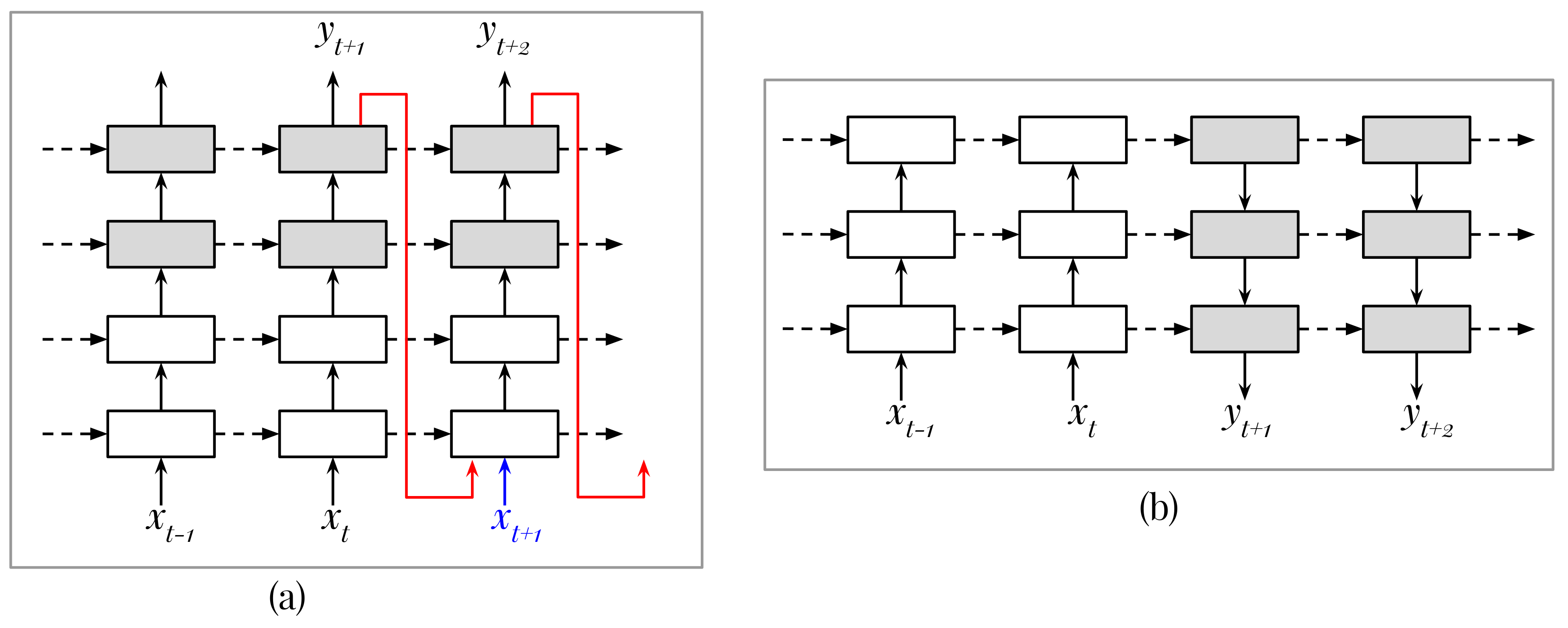
In practice, sequence-to-sequence network structures with several to many stacked recurrent layers are used to leverage the power of ConvRNN methods. Figure 2 illustrates two main structures, including Iterative Multi-step Estimation (IME, Figure 2a) and Direct Multi-step Estimation (DME, Figure 2b) [22]. In an IME model, encoding and decoding components are placed vertically as stacked layers, and at each input step there is an output. To predict the next step in a multi-step prediction fashion, an input is always needed. In training, ground-truth can be used as the input for that purpose, but, in testing, the current output must be fed back into the network. To reduce potential problems when the model sees good data in the training phase but degraded data in the testing phase, a common practice is to selectively feed the output back into the model in the training phase [22,27]. Meanwhile, in a DME model, the encoder and decoder are placed horizontally. In this design, the vertical directions of the encoder and decoder are contradictory [4,8,22]. By this way, layers of the same abstract level in the encoder and decoder are connected naturally, and there is no need to feed the current output back into the network for producing the next output. The three models ConvLSTM, ConvGRU and TrajGRU usually follow the IME structure [22].
Recent advances in ConvRNNs include the introduction of external memory, PredRNN and PredRNN++. The PredRNN architecture contains several stacked layers and one external memory, each layer contains one ConvLSTM cell that is connected to that external memory through several gates [16]. By this way, the cell accesses to two memories, one horizontally and one vertically, so that it can “remember” and update the spatial correlation (that the previous layers extract) as well as the temporal correlation (that the previous steps extract) at a time [16]. This is different to the simple ConvLSTM model, which just can recall and update the temporal correlation [16]. The PredRNN++ architecture incorporates more connections from the internal cell memory and the external memory, as well as a Gradient Highway Unit (GHU) to shorten the gradient from the output layer to the input layer [17]. Both of the PredRNN and PredRNN++ models are designed following the DME structure [22]. PredRNN is shown to be better than TrajGRU in both of the REE and video frame prediction tasks [16], and PredRNN++ is shown to be better than PredRNN in the video frame prediction task [17]. We noticed that PredRNN++ was not tested with the REE task [17]. Another work in this direction proposed to change the structure of ConvGRU and achieved better overall results than TrajGRU [24]. However, we noticed that it is worse than TrajGRU in predicting heavy rain [24].
2.1.2. 3D Radar Echo Extrapolation
As aforementioned in Section 1, traditional methods have been used to deal with the 3D REE task [1,12]. A related work proposed a 3D-radar-extrapolation method based on COTREC for precipitation nowcasting and showed that using 3D data are more accurate than only 2D data in forecasting fast growing storms [10]. The authors found that it is more advantageous with 3D nowcasting than 2D nowcasting in estimating the downward motions of precipitation particles in the mature and decaying stages of convective storms, especially with fast moving patterns. However, this approach still needs hand-crafted features, a noise reduction procedure, and specific domain knowledge, which may not be applicable in many cases. Moreover, the evaluation is done with data of only two events and the lead-time limitation is only 10 min. We argued that this time span is too short (so the changes are little and can be easily predicted) and two events are too little (so we did not know how the model would deal with uncertainty in many other events).
There are still very few works in the literature applying Deep Learning methods, particularly RNNs, for the 3D radar image prediction, despite of its importance. Several works have tried this research direction but are still limited and have not shown a clear picture. A work applied ConvLSTM for predicting multi-channels radar images by simply extending the dimensional space of the input and output data with an elevation dimension [11]. However, this is just a simple application of ConvLSTM, and there is no report about how the model works with the multi-channel prediction challenge. A more complicated work proposed 3D Successive Convolutional Network (3D-SCN) to fuse radar images from different observation stations and performed extrapolation [7]. Their findings in nowcasting convective storm provided more evidence to show that Deep Learning methods are better than traditional methods for the REE task. However, their methods are still based on CNN only, and they had to use fixed filters for a fixed length of input–output sequences [7]. This makes their method less flexible to necessary changes of prediction lengths, as well as unable to exploit long-distance correlations like LSTM-like models. In addition, the final output is a single channel image (composite reflectivity) rather than a 3D representation of data. Overall, these works do not investigate the new challenges that 3D prediction may pose to the convolution-based prediction models.
2.2. Data: Shenzen Radar Image Dataset
As mentioned above, we employed the Shenzen dataset provided by the Conference on Information and Knowledge Management (CIKM) Analytics Cup 2017 competition [18]. Each image covers an area of 101 × 101 km surrounding a certain weather observation site in the Shenzhen (Figure 3). Note that there are several sites taken into account, but, due to the competition, there is no detailed information about each of them. This dataset has 10,000 samples in the training set, and 4000 samples in the two test-sets, testA and testB [18]. Each sample is a sequence of 15 time steps (1 step = 6 min) of CAPPI radar images with four elevation-angles (0.5, 1.5, 2.5 and 3.5 km). Each image is of size (pixels), representing a resolution of km, which is considered as a convective scale [1]. The original range of pixel value is , but we normalized to . A histogram comparison of these sets is given in Figure 4, showing that the inconsistency of the train-set and the two test-sets is significant. Note that this characteristic is because the train-set is sampled in two consecutive years and the two test-sets are sampled within the next year. This characteristic is typical in weather data and poses a more challenging obstacle to the forecasting models than the cross-validation mechanism commonly used in machine learning, as the data distributions are different [3]. For calculating some operational evaluation metrics in the experiment, we converted the pixel space to the echo reflectivity space with an assumption of the gain and offset values (gain = 95, offset = 10) as used in [8]. By this way, the proportions of , and are , and , respectively. An important target of this study is to get high CSI and POD scores, and low FAR score for the last two types of rainfall, which are normal rain () and heavy rain ().
2.3. Methods
2.3.1. Data Augmentation
Firstly, in a search for simple Computer Vision tools which can improve the REE task, we investigated if using some common data augmentation techniques can help improve the generalization ability of RNN models. While this method is widely adopted in Computer Vision and Deep Learning [29] (Chapter 7), it has not been used to enhance the training process of neural networks in the precipitation nowcasting problem, and is rarely used in the neural networks-based Remote Sensing literature. However, there are some works in this field hinting at its usability for the REE task. For example, the interpolation technique is usually used to impute missing sensing data in the precipitation nowcasting problem [3,30]. For a Remote Sensing classification task, simple image augmentation techniques such as flipping, rotating and translating are shown to be helpful for improving deep convolutional models [31]. While this simple idea is not innovative, we seemed to be the first to fill the gap between the data augmentation techniques in Computer Vision and the radar-based REE task. We argued that this practice would help neural network models learn more patterns and changes in the training process, so that they could be more tolerant to uncertain changes in the future data.
In the training process, the image augmentation is performed with four steps as follows. Firstly, for each training mini-batch, 50% of samples were randomly selected for being augmented. Secondly, for a selected sample, the whole sequence will be transformed by one randomly selected operation among the set of {flipping up-down, flipping left-right, flipping up-down and flipping left-right, rotating 90 clockwise, rotating 90 counter-clockwise, rotating 90 clockwise and flipping up-down, rotating 90 clockwise and flipping left-right} widely used in the literature. Thirdly, again, 50% of the mini-batch are randomly selected to apply a reverse-order operation (reversing the selected sequences). In addition, finally, 50% are randomly selected to apply an illumination scale (scaling the brightness of the selected sequences). By applying each modifying operation on the whole sequence, we were able to enrich the spatial dynamics in the dataset but preserve the temporal dynamics. In addition, by reversing the order of image sequences, we were able to enrich the temporal dynamics but preserve the spatial dynamics. Note that the validating data were augmented by the same way too, but the testing data were not.
2.3.2. Channel-Wise Output Generation Block
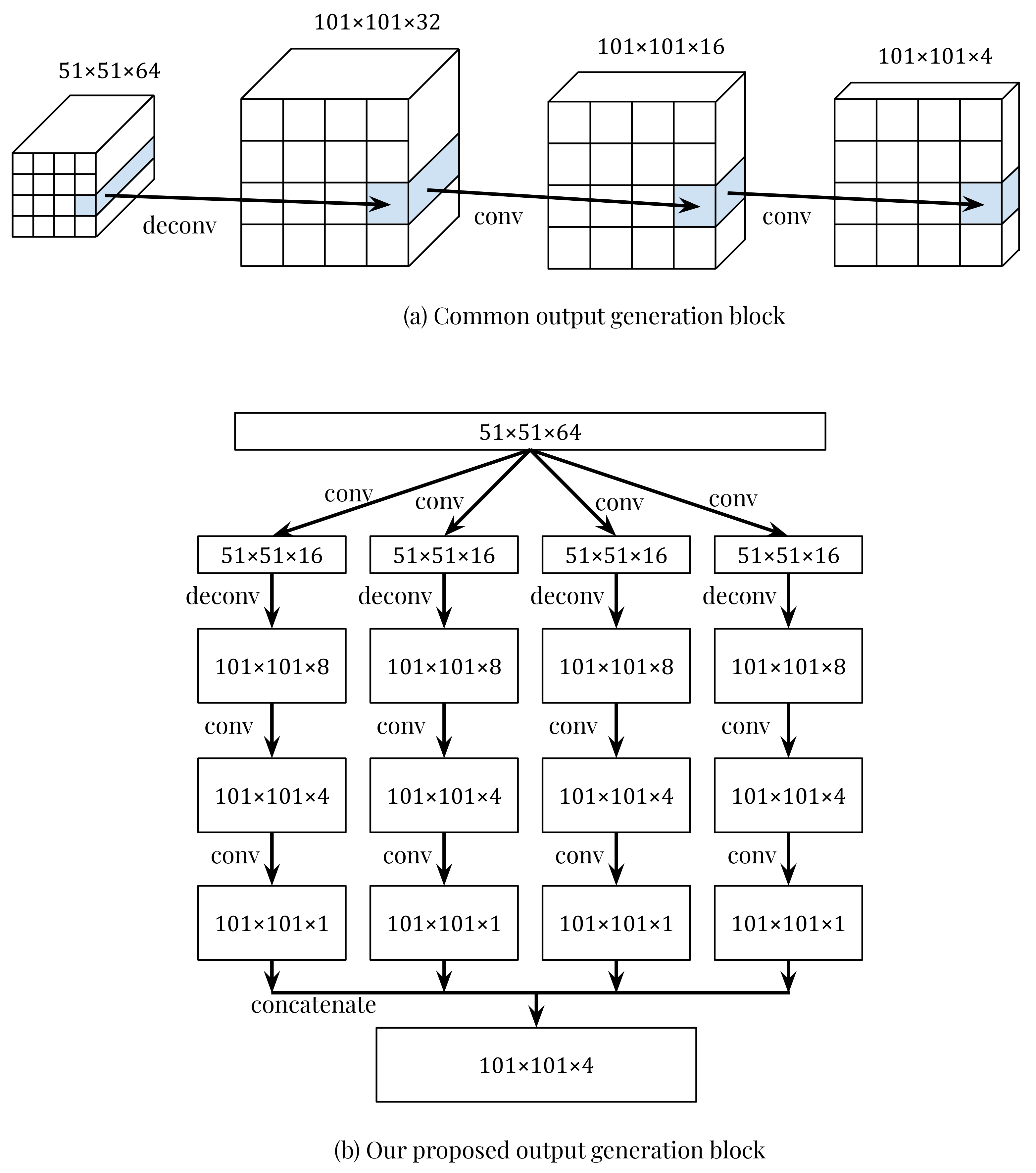
In our study, we employed both of the IME and DME structures, and adapted the proposed models in previous works to the Shenzen dataset (see Appendix A). We did not target altering the basis of these models but proposed new ways of applying them for improving the prediction quality. Our major contribution here is to investigate the output generation block, which produces from the last decoder cell. As we described in Section 1, if we simply extended the 2D models to the 3D models by increasing the number of channels of the final output, the cross-channel duplication, or cross-talk, problem would appear. To deal with this problem, we proposed to not use one set of convolution and deconvolution for all output channels but separate the generation of each channel as early as possible. Figure 5 illustrates this idea more clearly. In the common way (a), all output channels are generated by the same filter in each layer, meaning that the cross-channel information is directly taken into account in every transition. In our proposed way (b), each channel is generated with a separated set of filters, meaning that the cross-channel information is taken directly only in the first transition. After that, it is considered as indirect information and its side effects can be degraded gradually. Finally, after each single-channel image is generated, four images are concatenated to produce the expected shape. In this design, we used three convolution layers and one deconvolution layer to balance the performance and computing time, but one can stack more layers to reduce the cross-channel effect more. Note that, with this way, our output generation block can be easily generalized to any image sizes (and hence spatial scales of the REE task) by simply changing the sizes of convolutional kernels and feature maps.
3. Results
We performed experiments in TensorFlow [32] (version 1.8) on P100 Nvidia GPUs. With the data, we divided 10,000 samples in the train-set into 8000 for training and 2000 for validating (to specify the early-stopping point), and used 4000 samples in the test-sets for testing. In training, we used batch-size 4 (we saw that other bigger batch-sizes did not give better testing accuracy, and set the learning rate to start at and decreased it by a factor of after each 5 epochs. Similarly to Figure 1, we input seven steps and output eight steps (42 min of observation and 48 min of prediction, respectively). Even though this prediction time span is not long, we believed that it is enough to demonstrate the aspects we were focusing on. In addition, due to the fact that we initialized the weights of models with a random mechanism, we trained each model several times and chose the best one (similarly to [8]).
3.1. Data Augmentation
3.1.1. Training with L1 Loss
We compared several models proposed in the previous works, including ConvLSTM [3], ConvGRU [4], TrajGRU [4], PredRNN [16] and PredRNN++ [17], trained without and with data augmentation. All models were trained by only the MSE loss and early stopping strategy (after at least 10 epochs, or 20,000 weight-updating iterations, to allow PredRNN to converge stably). Results are presented in Table 1 and Table 2, respectively, following the viewpoint from Computer Vision used in [8]. The results provide very interesting findings. Firstly, it was clear that the data augmentation techniques helped improve the generalization with large margin for all models, especially in MSE (Table 3). It was also clear that the models trained without this support got over-fitted more severely. Secondly, PredRNN showed outstanding performance of all criteria over the previous models which do not have external memory, while PredRNN++ seemed to get over-fitted similarly to ConvLSTM. In terms of IQA metrics, PredRNN and PredRNN++ often outperformed the models without external memory. This means that the external memory mechanism was helpful to reduce the blurry image issue, which is consistent with the findings in [16,17]. Finally, the TrajGRU model seemed to not work well in this context while the ConvLSTM model got over-fitted more than the others in both cases.
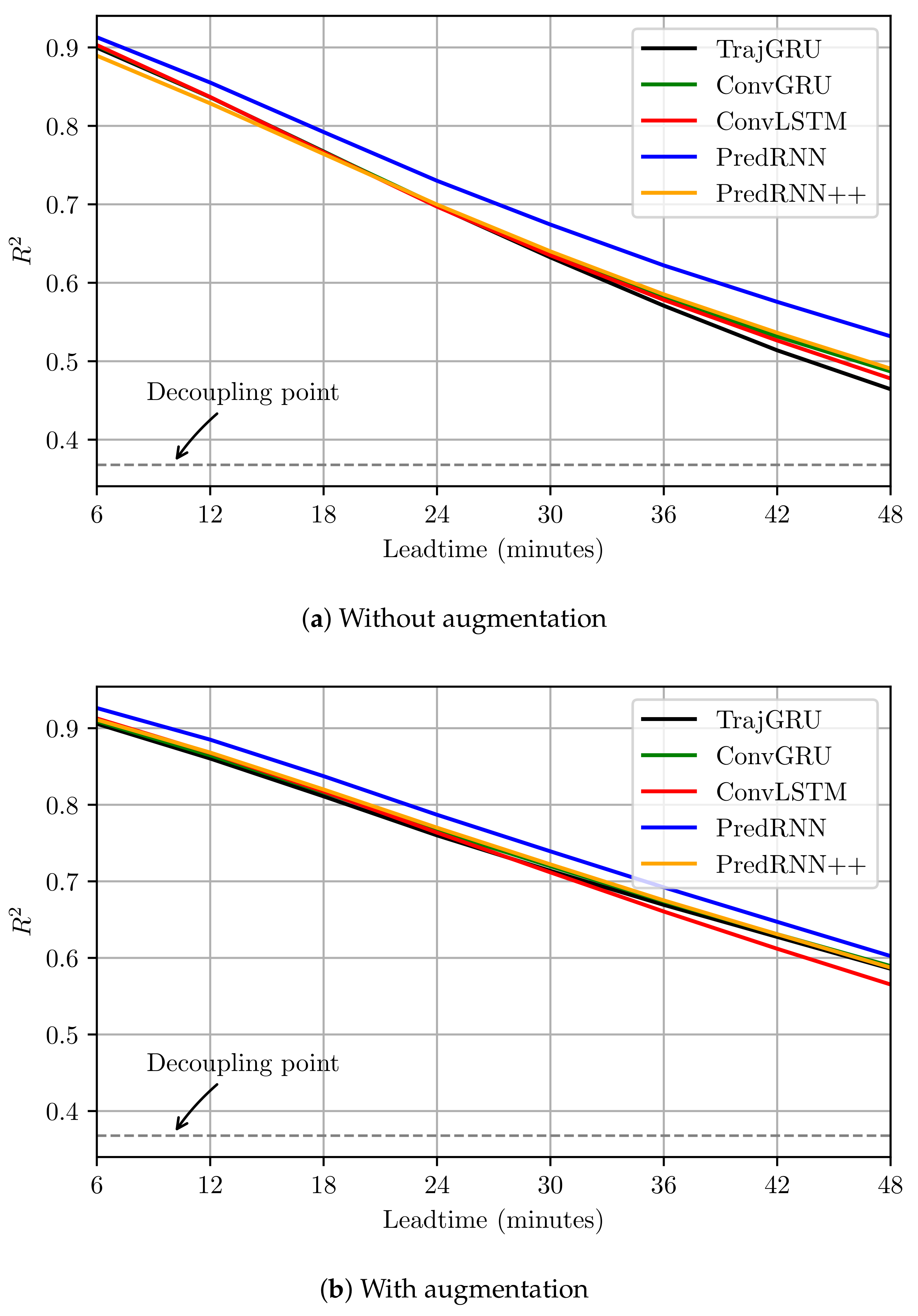
We investigated further into the effectiveness of data augmentation by plotting the step-wise coefficient of determination scores. As shown in Figure 6, it is interesting to see that the models trained with data augmentation had quite similar performance with the models trained without data augmentation for the first and second steps but were significantly better for the next steps.
3.1.2. Training with Combined Loss
In this experiment, we used a Combined Loss Function (CLF) based on MSE, MAE and SSIM for training the above models to obtain less blurry images [8]. We defined this CLF as:
Results are given in Table 4. As there was other information in the loss function, the MSE score got worse, but the overall accuracy was compensated by significant improvements of the MAE and SSIM scores. This means that the image quality was significantly improved and the blurry effect was reduced. In general, PredRNN and PredRNN++ were still better than the models without external memory. Since PredRNN still outperformed the others in all aspects, we concluded that it was the best model in the data context of this paper and would use it for further experiments. To confirm the relation between the learning iterations with the cross-talk effect, we also tried training this PredRNN model more to see if training longer could make the receptive field to learn to reduce this impact.
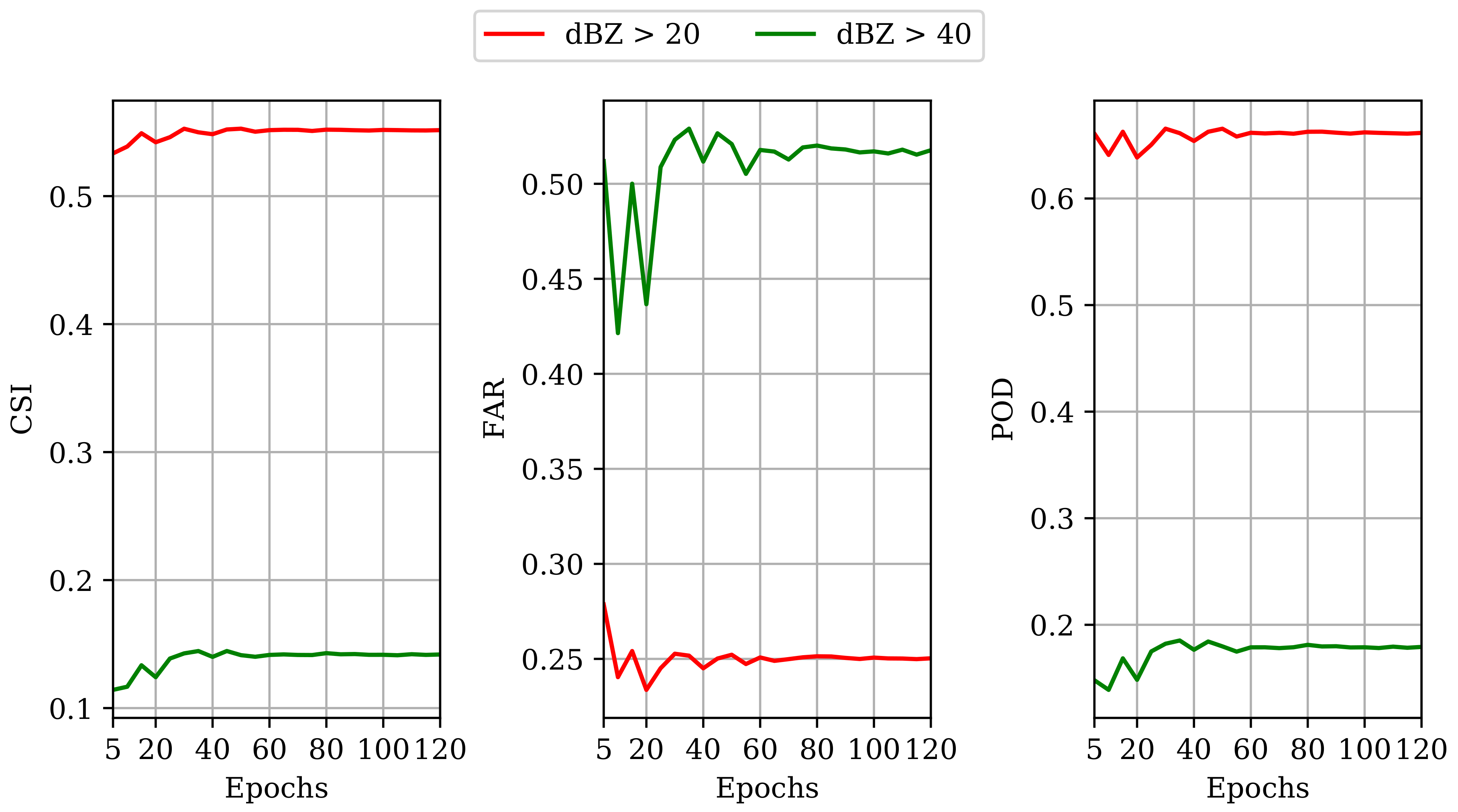
Figure 7 shows an example to illustrate this experimental finding. Intuitively, the observation error from the top channel appeared in other channels after both 15 and 80 training epochs like in Figure 1. This means that the cross-talk effect still appeared, even though we used different models and training loss functions, and still happened with other data samples. In addition, even though we trained the model longer, it still appeared (with lesser degree). Note that, in these processed images, some parts of the precipitation particles can be missed due to the changes in intensity, contrast and brightness (original images are given in Figure A1, Appendix B). In particular, if the error signal has high intensity while other channels are low intensity, the estimation of low intensity particles in those channels will be affected severely. We also saw that the practice of training more did not solve this issue completely, but led to another problem, the over-fitting issue. We illustrated this finding by plotting the CSI, FAR and POD scores against training epochs (for two important cases: and ) in Figure 8. In general, it can be said that, after around 35 to 40 training epochs, these operational expectations did not get better, or even got worse. Hence, it was problematic to solve the cross-talk issue by increasing the number of training iterations, and we had to use another solution here, changing the output generation block.
3.2. Output Generation Blocks
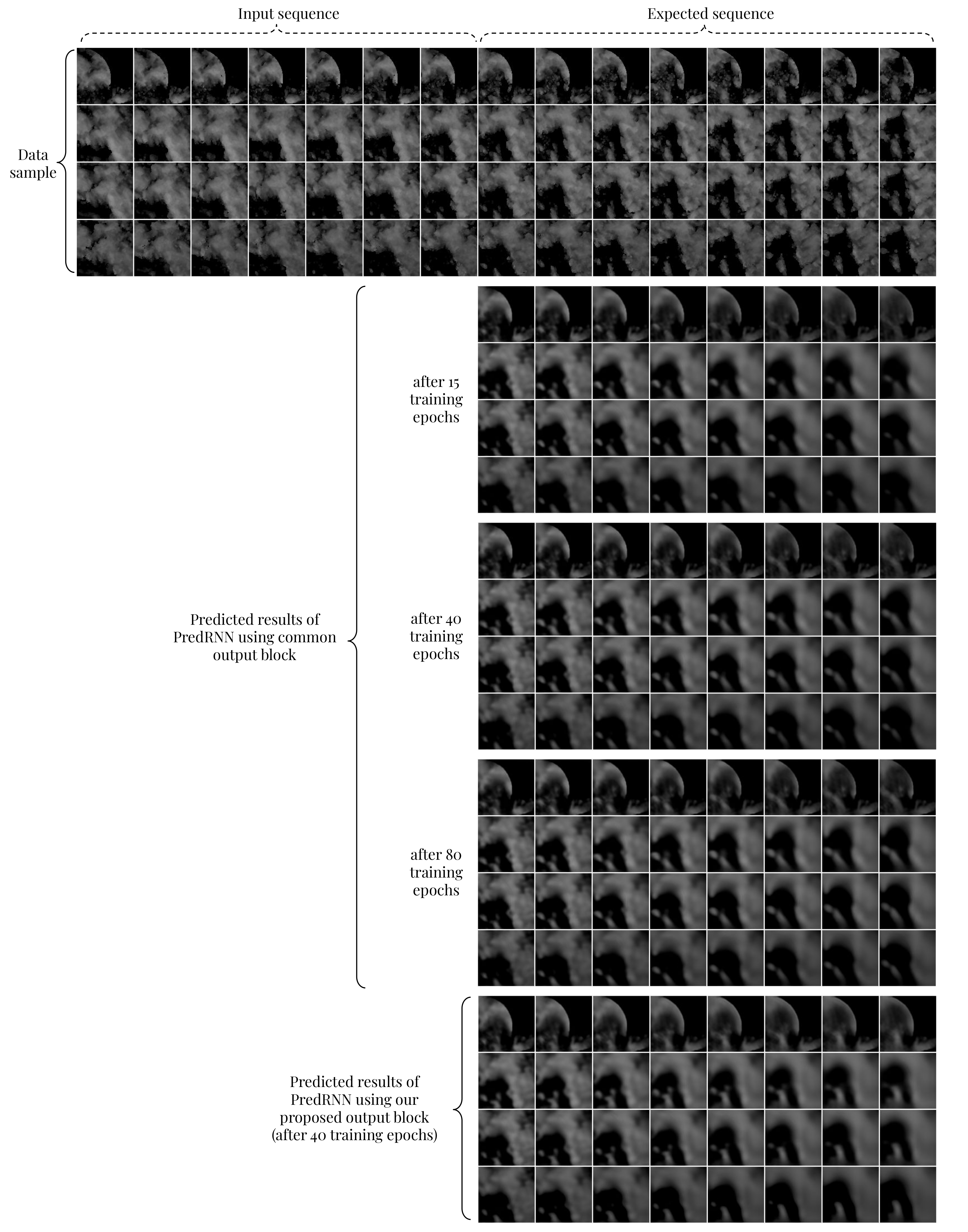
In this experiment, which is the most important part of our work, we chose the above PredRNN model but combined it with different output generation blocks described in Figure 5 and trained it with the CLF. Our intention was to show that the proposed output generation block could be a worthy alternative to the common convolutional mechanism to reduce the cross-talk issue, but still able to take advantages of the early-stopping technique to avoid the over-fitting problem. For a fair comparison in terms of training iterations, we chose to report the results of each model after 40 training epochs here. The example in Figure 9 illustrates the differences between the two PredRNN models. Intuitively, the model with our proposed output block significantly reduced the cross-talk effect. Especially in the top-second and bottom channels, this effect almost disappeared. In addition, we saw that this result was even better than the result provided by the model using the common output block trained for 80 epochs. Note that we also tried this experiment with other ConvRNN models and saw similar results (of course with lower accuracy than the PredRNN model).
To confirm that our proposed method did not cause unexpected side effects to the overall prediction quality, we took a look at the testing criteria of Computer Vision and operational expectations, as shown in Table 5 and Table 6, respectively. As we expected, our proposed output generation block did not cause a significantly negative effect, and even slightly improved the overall prediction quality (of course not always). In particular, in terms of operational criteria, our output generation block seemed to be more stable with medium to heavy rainfall events. From the example in Figure 9, we noticed that this could be because our output block might preserve the higher intensity slightly better. From these findings, we could argue that our proposed method is competitive enough to be applied in practice.
4. Discussion
Firstly, we discussed the success of using some simple image data augmentation techniques in Computer Vision for training the REE models. Even though the variations of added images are simple, they enriched the number of patterns in the training set. This allowed the models to be exposed to more uncertainty before they were used for testing. The fact that the models trained with data augmentation obtained higher validating error but lower testing error means that the over-fitting problem was significantly reduced. From Figure 6, we noticed that this improvement was similar to the dec-seq2seq model structure proposed in [8]. However, we argued that using the data augmentation can be safer and more stable because it increases the number of patterns to a countless extent and allows big models to remember these patterns, rather than using smaller models and causes a limitation in the memorizing ability. We therefore believed that data augmentation is a good solution to deal with the high uncertainty in weather data in general, not only radar data. Furthermore, we also argued that the generalization ability of precipitation nowcasting models can be enhanced more with more complicated augmentation techniques in Computer Vision, such as GAN, but would leave this investigation as a future work.
Secondly, we discussed the outstanding performance of PredRNN in our experiments. From Table 1, Table 2 and Table 4, this model consistently outperformed others in all testing criteria. This finding is consistent with the claim that PredRNN is better than ConvLSTM stated in [16], but opposite to the claim that PredRNN++ is better than PredRNN stated in [17]. However, we noticed that, while the former comparison is done with the REE task, the latter one is done merely on tasks of prediction of video frames or moving digits data. Therefore, here we contributed another clear comparison of these two models for the REE literature. We believed that the external memory mechanism of PredRNN did help capture information and explore new patterns better than ConvLSTM, ConvGRU and TrajGRU (note that PredRNN++ was also better than these three models). On the other hand, it seemed that the architecture of PredRNN++ is too complicated and could not be trained well in the context of our employed data. Table 1 showed that it was less accurate than PredRNN in both training and testing, while Table 2 and Table 4 showed that it was more over-fitted. In addition, from a comparison of network sizes inferred from Table A1, at first, we thought that PredRNN was less over-fitted because it had the least number of trainable parameters. However, when we tried reducing the number of channels in the abstract levels as done in [8], we saw results that were a little worse than all of the current models. We also tried setting the number of channels of ConvLSTM, ConvGRU and TrajGRU as to reduce their size but still saw the same situation. Therefore, we concluded that PredRNN outperformed the others because of its characteristics, which might be more suitable to the dataset, rather than because of the network size.
Thirdly, we discussed the cross-talk effect. Unfortunately, even the best model, PredRNN, still had the problem of cross-channel duplication of information, especially with the samples in which observation errors are severe (similarly to the example in Figure 1). In fact, we saw this effect with a similar degree in the results of all employed models. Therefore, we could confirm that the cross-talk effect is an inherent shortcoming of all of these models, as hypothesized previously. We realized that this issue could be even more severe with PredRNN than ConvGRU (and other models without external memory) because the external memory could bring detailed information of the observation errors from low abstract levels to high abstract levels directly. The results from Section 3.2 showed that our proposed output generation block could deal with this issue well. This can be explained easily as it is thanks to the early separation of information of channels. Moreover, this finding can help promote the application of PredRNN (or PredRNN++) in many multi-channel prediction tasks. However, we must admit that the cross-talk issue still appeared in our best model, and argued that it could be reduced more with a deeper output generation block. In addition, we believed that this effect is unavoidable because we have to balance between the depth of the output generation block and the computing cost, which can increase when adding more transition layers. Despite this fact, we thought that the current design of our output generation block is enough to demonstrate our idea in dealing with this issue.
Finally, besides those achievements, there are some points that need to be investigated more. A drawback of our proposed output block is that one must initiate many sets of convolutions and deconvolutions when there are many channels, e.g.,: 20 elevation angles are corresponding to 20 sets of filters. This would increase the number of trainable variables significantly. However, we argued that, if using the common way in such case, the cross-talk effect may be more severe, and training neural networks can be more difficult. For future work, we thought that testing this argument would be an interesting direction. We also propose to test our generation block with longer sequences (e.g., 20 input steps and 20 output steps), and with a multi-radar multi-channel data source. It is also important to find a suitable way to quantitatively assess the cross-talk effect (e.g., template-matching or pattern matching in Computer Vision). Finally, a framework for automatically choosing appropriate method(s), network structures, and hyper-parameters will be another interesting research direction.
5. Conclusions
This paper has presented a part of our study on using recent advanced tools in Deep Learning and Computer Vision for the problem of radar-based precipitation nowcasting. Our main contribution is an investigation into adapting ConvRNN models for the 3D REE task. Most importantly, we showed that the cross-talk problem can appear when applying the same convolutional mechanism of the 2D prediction models for the 3D prediction task. We discussed several aspects that should be considered surrounding this problem such as the number of learning iterations and the early termination of the training process. To deal with the cross-talk effect, we proposed a promising solution, a novel output generation block which separates the generation of each channel as early as possible. While the overall performance of using our proposed output block is not clearly better than the common way, we believed that the reduction of the cross-talk effect would reduce the uncertainty in operational contexts. As we argued, it is able to promote PredRNN or other external-memory-based ConvRNN methods in the context of 3D radar data prediction, since the external memory may cause this effect to be more severe. We also showed that common data augmentation techniques in Computer Vision are helpful for dealing with high uncertainty in weather radar data. Even though our experiments were done with a quite limited sequence length, the adopted settings can be useful in nowcasting phenomena like thunderstorms or hails, for which real-time responding models are critically needed.
Author Contributions
Q.-K.T. collected the data, developed the model, and designed and performed the experiments. Q.-K.T. and S.-k.S. analyzed the results. Q.-K.T. wrote the paper. S.-k.S. provided the overall guidance to the study, and reviewed and edited the manuscript.
Funding
This research was funded by Korea Institute of Science and Technology Information (KISTI), project “Construction of Research Data Open Platform and its Utilization Support”, Project No.: K-19-L01-C04. The APC was funded by the same source.
Acknowledgments
We thank Jung-Ho Uhm, Seongchan Kim and Ph.D candidate Seungkyun Hong in KISTI for their great support and discussions. Finally, we thank the organizers of CIKM AnalytiCup 2017 for sharing their data freely.
Conflicts of Interest
The authors declare no conflict of interest.
Appendix A. Description of Models
Table A1 below summarizes the description of models used in our experiment. We constructed ConvLSTM, ConvGRU and TrajGRU following the DME structure (Figure 2b), with three recurrent layers in both of the encoder and decoder. The numbers of channels in the layers are from bottom to top. Whilst PredRNN and PredRNN++ are constructed following the IME structure (Figure 2a), with two encoding layers () and two decoding layers (). Note that the feature map sizes of layers in PredRNN and PredRNN++ are not changed, so we used dilation in high abstract levels to allow receptive fields to “see” broader views. Following [16,17], we used the function to activate switching gates (for choosing which signals are turned on or off) and the function to activate gate operations in all cells. In all models, before feeding data into the encoder, the input image of shape is convolved by a receptive field of size to result in a feature map of shape . Moreover, to produce the final output, one deconvolution and two convolutions are used to transfer the state of shape to the original image of shape (Figure 5a). This process is where we proposed to use our output generation block (Figure 5b) to improve the image quality. Note that we used the leaky-ReLU function to activate these final operations.

Table A1.
Structures and characteristics of models.
| Model | Structure | Channels of Layers/Feature Map Sizes | Recurrent Operations | Number of Variables | Number of Parameters |
|---|---|---|---|---|---|
| ConvLSTM | DME | 8 map: | conv: k = [5, 5, 3] | 50 | 9,383,760 |
| ConvGRU | DME | map: | conv: k = [5, 5, 3] | 32 | 5,918,800 |
| TrajGRU | DME | map: | flow generation: k = 5, c = 32; warping: L = [13, 13, 9] | 61 | 5,452,572 |
| PredRNN | IME | map: | conv: k = [5, 5, 5, 5] dilation: r = [1, 2, 2, 1] | 39 | 4,648,464 |
| PredRNN++ | IME | GHU (GHU: s = 64, k = 5) map: | conv: k = [5, 5, 5, 5] dilation: r = [1, 2, 2, 1] | 50 | 7,106,192 |
Notations: k: kernel size ([ ] is an array of layers’ kernel sizes); c and L: number of channels and number of neighbouring points, respectively, of the flow generation network in TrajGRU cells; s: number of channels in GHU block; r: dilation rate.
Appendix B. Data Sample and Predicted Examples

References
- Pierce, C.; Seed, A.; Ballard, S.; Simonin, D.; Li, Z. Nowcasting. In Doppler Radar Observations-Weather Radar, Wind Profiler, Ionospheric Radar, and Other Advanced Applications; IntechOpen: Rijeka, Croatia, 2012. [Google Scholar] [Green Version]
- Shi, E.; Li, Q.; Gu, D.; Zhao, Z. A Method of Weather Radar Echo Extrapolation Based on Convolutional Neural Networks. In Lecture Notes in Computer Science, Proceedings of the MultiMedia Modeling (MMM 2018), Bangkok, Thailand, 5–7 February 2018; Schoeffmann, K., Chalidabhongse, T.H., Ngo, C.W., Aramvith, S., O’Connor, N.E., Ho, Y.-S., Gabbouj, M., Elgammal, A., Eds.; Springer: Cham, Switzerland, 2018; Volume 10704, pp. 16–28. [Google Scholar] [CrossRef]
- Shi, X.; Chen, Z.; Wang, H.; Yeung, D.Y.; Wong, W.K.; Woo, W.C. Convolutional LSTM Network: A Machine Learning Approach for Precipitation Nowcasting. In Proceedings of the Advances in Neural Information Processing Systems (NIPS), Montreal, QC, Canada, 7–12 December 2015; pp. 802–810. [Google Scholar]
- Shi, X.; Gao, Z.; Lausen, L.; Wang, H.; Yeung, D.Y.; Wong, W.K.; Woo, W.C. Deep Learning for Precipitation Nowcasting: A Benchmark and a New Model. In Proceedings of the Advances in Neural Information Processing Systems (NIPS), Long Beach, CA, USA, 4–9 December 2017; pp. 5617–5627. [Google Scholar]
- Woo, W.; Shi, X.; Yeung, D.-Y.; Woo, W.-C. A Deep-Learning Method for Precipitation Nowcasting. In Proceedings of the International Symposium on Nowcasting and Very-Short-Range Forecast, Hong Kong, China, 25–29 July 2016. [Google Scholar]
- Asanjan, A.A.; Yang, T.; Hsu, K.; Sorooshian, S.; Lin, J.; Peng, Q. Short-term Precipitation Forecast based on the PERSIANN system and the Long ShortTerm Memory (LSTM) Deep Learning Algorithm. J. Geophys. Res. Atmos. 2018. [Google Scholar] [CrossRef]
- Zhang, W.; Han, L.; Sun, J.; Guo, H.; Dai, J. Application of multi-channel 3D-cube successive convolution network for convective storm nowcasting. arXiv 2017, arXiv:1702.04517. [Google Scholar]
- Tran, Q.K.; Song, S.K. Computer Vision in Precipitation Nowcasting: Applying Image Quality Assessment Metrics for Training Deep Neural Networks. Atmosphere 2019, 10, 244. [Google Scholar] [CrossRef]
- Jang, B.J.; Lim, S.; Lee, K.H.; Lee, C.; Kim, W. GIS Based Realistic Weather Radar Data Visualization Technique. J. Multimed. Inf. Syst. 2017, 4, 1–8. [Google Scholar]
- Otsuka, S.; Tuerhong, G.; Kikuchi, R.; Kitano, Y.; Taniguchi, Y.; Ruiz, J.J.; Satoh, S.; Ushio, T.; Miyoshi, T. Precipitation nowcasting with three-dimensional space-time extrapolation of dense and frequent phased-array weather radar observations. Weather Forecast. 2016, 31, 329–340. [Google Scholar] [CrossRef]
- Heye, A.; Venkatesan, K.; Cain, J. Precipitation Nowcasting: Leveraging Deep Recurrent Convolutional Neural Networks. In Proceedings of the Cray User Group (CUG) 2017—Caffeinated Computing, Redmond, WA, USA, 8–11 May 2017. [Google Scholar]
- Rinehart, R.; Garvey, E. Three-dimensional storm motion detection by conventional weather radar. Nature 1978, 273, 287. [Google Scholar] [CrossRef]
- Kim, Y.; Maki, M.; Lee, D.I.; Jeong, J.H.; You, C.H. Three-dimensional analysis of the initial stage of convective precipitation using an operational X-band polarimetric radar network. Atmos. Res. 2019, 225, 45–57. [Google Scholar] [CrossRef]
- McGovern, A.; Elmore, K.L.; Gagne, D.J.; Haupt, S.E.; Karstens, C.D.; Lagerquist, R.; Smith, T.; Williams, J.K. Using artificial intelligence to improve real-time decision-making for high-impact weather. Bull. Am. Meteorol. Soc. 2017, 98, 2073–2090. [Google Scholar] [CrossRef]
- Tran, Q.K. Prediction of Multidimensional Weather Radar Image Sequences Using Convolutional Recurrent Neural Networks. Unpublished Ph.D. Thesis, University of Science and Technology (UST), Daejeon, Korea, 2019. [Google Scholar]
- Wang, Y.; Long, M.; Wang, J.; Gao, Z.; Philip, S.Y. PredRNN: Recurrent Neural Networks for Predictive Learning Using Spatiotemporal LSTMs. In Proceedings of the Advances in Neural Information Processing Systems (NIPS), Long Beach, CA, USA, 4–9 December 2017; pp. 879–888. [Google Scholar]
- Wang, Y.; Gao, Z.; Long, M.; Wang, J.; Yu, P.S. PredRNN++: Towards a Resolution of the Deep-in-Time Dilemma in Spatiotemporal Predictive Learning. In Proceedings of the International Conference on Machine Learning (ICML), Stockholm, Sweden, 10–15 July 2018. [Google Scholar]
- CIKM AnalytiCup 2017 Dataset. Available online: https://tianchi.aliyun.com/dataset/dataDetail?dataId=1085 (accessed on 17 September 2019).
- Bickel, D.; Doerry, A. Measuring Channel Balance in Multi-Channel Radar Receivers. In Proceedings of the Radar Sensor Technology XXII, International Society for Optics and Photonics, Ballroom Level, Osceola, Orlando, FL, USA, 16–18 April 2018; Volume 10633, p. 106331A. [Google Scholar]
- Ośródka, K.; Szturc, J.; Jakubiak, B.; Jurczyk, A. Processing of 3D weather radar data with application for assimilation in the NWP model. Misc. Geogr. 2014, 18, 31–39. [Google Scholar] [CrossRef]
- Buszta, A.; Mazurkiewicz, J. Climate Changes Prediction System Based on Weather Big Data Visualisation. In Proceedings of the International Conference on Dependability and Complex Systems, Brunów, Poland, 29 June–3 July 2015; pp. 75–86. [Google Scholar]
- Shi, X.; Yeung, D.Y. Machine Learning for Spatiotemporal Sequence Forecasting: A Survey. arXiv 2018, arXiv:1808.06865. [Google Scholar]
- Singh, S.; Sarkar, S.; Mitra, P. A Deep Learning Based Approach with Adversarial Regularization for Doppler Weather Radar ECHO Prediction. In Proceedings of the IEEE International Geoscience and Remote Sensing Symposium (IGARSS), Fort Worth, TX, USA, 23–28 July 2017; pp. 5205–5208. [Google Scholar]
- Sato, R.; Kashima, H.; Yamamoto, T. Short-Term Precipitation Prediction with Skip-Connected PredNet. In Lecture Notes in Computer Science, Proceedings of the ICANN 2018: Artificial Neural Networks and Machine Learning, Rhodes, Greece, 4–7 October 2018; Kůrková, V., Manolopoulos, Y., Hammer, B., Iliadis, L., Maglogiannis, I., Eds.; Springer: Cham, Switzerland, 2018; Volume 11141, pp. 373–382. [Google Scholar] [CrossRef]
- Tan, C.; Feng, X.; Long, J.; Geng, L. FORECAST-CLSTM: A New Convolutional LSTM Network for Cloudage Nowcasting. In Proceedings of the 2018 IEEE Visual Communications and Image Processing (VCIP), Taichung, Taiwan, 9–12 December 2018; pp. 1–4. [Google Scholar]
- Kim, S.; Kim, H.; Lee, J.; Yoon, S.; Kahou, S.E.; Kashinath, K.; Prabhat, M. Deep-Hurricane-Tracker: Tracking and Forecasting Extreme Climate Events; Technical Report; Lawrence Livermore National Lab. (LLNL): Livermore, CA, USA, 2018.
- Srivastava, N.; Mansimov, E.; Salakhudinov, R. Unsupervised Learning of Video Representations Using Lstms. In Proceedings of the International Conference on Machine Learning, Lille, France, 6–11 July 2015; pp. 843–852. [Google Scholar]
- Meteorological Bureau of Shenzhen Municipality’s Website. Available online: http://weather.sz.gov.cn/en/en_shenzhentianqi/ (accessed on 17 September 2019).
- Goodfellow, I.; Bengio, Y.; Courville, A. Regularization for Deep Learning. In Deep Learning; MIT Press: Cambridge, MA, USA, 2016; Chapter 7; pp. 233–234. [Google Scholar]
- Sigrist, F.; Künsch, H.R.; Stahel, W.A. A dynamic nonstationary spatio-temporal model for short term prediction of precipitation. Ann. Appl. Stat. 2012, 6, 1452–1477. [Google Scholar] [CrossRef]
- Yu, X.; Wu, X.; Luo, C.; Ren, P. Deep learning in remote sensing scene classification: A data augmentation enhanced convolutional neural network framework. GISci. Remote Sens. 2017, 54, 741–758. [Google Scholar] [CrossRef]
- Abadi, M.; Barham, P.; Chen, J.; Chen, Z.; Davis, A.; Dean, J.; Devin, M.; Ghemawat, S.; Irving, G.; Isard, M.; et al. TensorFlow: A System for Large-Scale Machine Learning. In Proceedings of the 12th USENIX Symposium on Operating Systems Design and Implementation (OSDI 16), Savannah, GA, USA, 2–4 November 2016; pp. 265–283. [Google Scholar]
Figure 1.
Example of preliminary results of ConvGRU over the Shenzen dataset. (a): the first four rows are four channels of a tested sample with 15 steps (seven input steps and eight expected output steps); in the first channel, the radar beam blockage causes observation error (but this error does not appear in other channels); the last four rows are predicted images produced after 15 training epochs; (b): we processed these images to show the cross-talk effect more clearly by changing the luminosity (both brightness and contrast); (c): the processed prediction after 80 training epochs, showing that the cross-talk effect was significantly reduced.

Figure 2.
Two main types of sequence-to-sequence structures of ConvRNN models for the REE task in precipitation nowcasting (adapted from [22]). (a): Iterative Multi-step Estimation. (b): Direct Multi-step Estimation. The encoder cells are white while the decoder cells are gray. In (a), the red color arrow-lines illustrate the feeding-back operation in the testing phase. In the training phase, this operation can be used selectively to replace the real input (blue color). In (b), this operation is not needed. Basically, on the vertical direction, the encoder uses convolutions (often with stride size >1) and the decoder uses deconvolutions. Moreover, in practice, convolutional layers are usually used to extract feature maps from the raw input before feeding them into the bottom recurrent layer, and deconvolutional layers are used to reconstruct the original shape—best view in color.

Figure 3.
The study region: Left: location of the Shenzhen, China (source: Google Maps); Right: some weather observation sites in Shenzhen (source: Meteorological Bureau of Shenzhen Municipality’s website [28]). Some of them may be used in the CIKM Analytics Cup 2017 competition [18], but, due to the competition policies, the organizer did not reveal which ones—best view in color.

Figure 4.
Histograms of non-zero pixel values in the dataset (divided into three parts: train, testA and testB)—best view in color.
Figure 4.
Histograms of non-zero pixel values in the dataset (divided into three parts: train, testA and testB)—best view in color.

Figure 5.
Two types of output generation blocks for producing four channels of radar images at a time. For convenience, the layer-to-layer transitions in (a) are presented horizontally (in fact, the arrows in the both sub-figures have the same direction).
Figure 5.
Two types of output generation blocks for producing four channels of radar images at a time. For convenience, the layer-to-layer transitions in (a) are presented horizontally (in fact, the arrows in the both sub-figures have the same direction).

Figure 6.
Step-wise coefficient of determination score (R2) of models trained with and without data augmentation—best view in color.
Figure 6.
Step-wise coefficient of determination score (R2) of models trained with and without data augmentation—best view in color.

Figure 7.
Example of a tested prediction of the PredRNN model trained with the
. We processed the images to make the duplicated parts emerge clearly (see the original ones in
Figure A1). Different to Figure 1, we chose this sample to show that the error signal in a channel might affect the estimation of edges of precipitation particles in other channels.

Figure 8.
Variations of operational nowcasting metrics on the test-set provided by PredRNN over two rain-rate thresholds ( and ) against training epochs.
Figure 8.
Variations of operational nowcasting metrics on the test-set provided by PredRNN over two rain-rate thresholds ( and ) against training epochs.

Figure 9.
Example of predicted results of PredRNN models (after 40 training epochs) using the common output block (a) and our proposed output block (b). Original images are given in Figure A1.
Figure 9.
Example of predicted results of PredRNN models (after 40 training epochs) using the common output block (a) and our proposed output block (b). Original images are given in Figure A1.

Table 1.
Test results of models trained without data augmentation.
| Model | Validating | Testing | ||||
|---|---|---|---|---|---|---|
| MSE | MSE | MAE | SSIM | MS-SSIM | PCC | |
| Last input | - | 1.7379 | 0.7990 | 0.4568 | 0.4675 | 0.7005 |
| TrajGRU | 0.4397 | 0.9804 | 0.6382 | 0.5008 | 0.5951 | 0.8154 |
| ConvGRU | 0.3172 | 0.9688 | 0.6201 | 0.5223 | 0.6002 | 0.8205 |
| ConvLSTM | 0.3203 | 0.9825 | 0.6223 | 0.5227 | 0.6047 | 0.8187 |
| PredRNN | 0.3271 | 0.8686 | 0.5786 | 0.5524 | 0.6398 | 0.8403 |
| PredRNN++ | 0.3588 | 0.9654 | 0.6230 | 0.5230 | 0.6021 | 0.8202 |
MSE: Mean Squared Error; MAE: Mean Absolute Error; SSIM: Structural SIMilarity; MS-SSIM: Multi-Scale SSIM; PCC: Pearson’s Correlation Coefficient.
Table 2.
Test results of models trained with data augmentation.
| Model | Validating | Testing | ||||
|---|---|---|---|---|---|---|
| MSE | MSE | MAE | SSIM | MS-SSIM | PCC | |
| TrajGRU | 0.7207 | 0.7528 | 0.5741 | 0.5110 | 0.6503 | 0.8590 |
| ConvGRU | 0.6241 | 0.7383 | 0.5579 | 0.5362 | 0.6633 | 0.8617 |
| ConvLSTM | 0.5794 | 0.7650 | 0.5647 | 0.5283 | 0.6659 | 0.8569 |
| PredRNN | 0.6473 | 0.6918 | 0.5313 | 0.5545 | 0.6920 | 0.8713 |
| PredRNN++ | 0.5733 | 0.7409 | 0.5501 | 0.5467 | 0.6738 | 0.8627 |
Table 3.
Detailed improvement of the testing metrics obtained by using data augmentation.
| Model | MSE | MAE | SSIM | MS-SSIM | PCC | Average |
|---|---|---|---|---|---|---|
| TrajGRU | 23.22% | 10.04% | 2.04% | 9.28% | 5.35% | 9.98% |
| ConvGRU | 23.79% | 10.03% | 2.66% | 10.51% | 5.02% | 10.40% |
| ConvLSTM | 22.14% | 9.26% | 1.07% | 10.12% | 4.67% | 9.45% |
| PredRNN | 20.35% | 8.17% | 0.38% | 8.16% | 3.69% | 8.15% |
| PredRNN++ | 23.25% | 11.70% | 4.53% | 11.91% | 5.18% | 11.32% |
Table 4.
Test results of models trained with data augmentation.
| Model | Validating | Testing | ||||
|---|---|---|---|---|---|---|
| CLF | MSE | MAE | SSIM | MS-SSIM | PCC | |
| TrajGRU | 0.6367 | 0.7672 | 0.5341 | 0.5965 | 0.6672 | 0.8583 |
| ConvGRU | 0.5796 | 0.7809 | 0.5338 | 0.5987 | 0.6683 | 0.8568 |
| ConvLSTM | 0.5562 | 0.7715 | 0.5258 | 0.6063 | 0.6729 | 0.8586 |
| PredRNN | 0.5841 | 0.7492 | 0.5201 | 0.6087 | 0.6789 | 0.8633 |
| PredRNN++ | 0.5727 | 0.7734 | 0.5273 | 0.6063 | 0.6752 | 0.8589 |
CLF: Combined Loss Function.
Table 5.
Comparison of the common output block and our output block over Computer Vision criteria (after 40 epochs of training).
Table 5.
Comparison of the common output block and our output block over Computer Vision criteria (after 40 epochs of training).
| Model | Validating | Testing | ||||
|---|---|---|---|---|---|---|
| CLF | MSE | MAE | SSIM | MS-SSIM | PCC | |
| PredRNN (common block) | 0.5884 | 0.7492 | 0.5206 | 0.6087 | 0.6783 | 0.8632 |
| PredRNN (our block) | 0.5964 | 0.7481 | 0.5212 | 0.6081 | 0.6788 | 0.8633 |
Table 6.
Comparison of the common output block and our output block over operational criteria.
| Testing Metric | Method | dBZ Threshold | ||
|---|---|---|---|---|
| 5 | 20 | 40 | ||
| CSI | Common block | 0.7418 | 0.5484 | 0.1400 |
| Our block | 0.7413 | 0.5499 | 0.1403 | |
| FAR | Common block | 0.1290 | 0.2451 | 0.5117 |
| Our block | 0.1300 | 0.2421 | 0.4950 | |
| POD | Common block | 0.8201 | 0.6540 | 0.1766 |
| Our block | 0.8204 | 0.6526 | 0.1774 | |
© 2019 by the authors. Licensee MDPI, Basel, Switzerland. This article is an open access article distributed under the terms and conditions of the Creative Commons Attribution (CC BY) license (http://creativecommons.org/licenses/by/4.0/).
Share and Cite
MDPI and ACS Style
Tran, Q.-K.; Song, S.-k. Multi-Channel Weather Radar Echo Extrapolation with Convolutional Recurrent Neural Networks. Remote Sens. 2019, 11, 2303. https://doi.org/10.3390/rs11192303
AMA Style
Tran Q-K, Song S-k. Multi-Channel Weather Radar Echo Extrapolation with Convolutional Recurrent Neural Networks. Remote Sensing. 2019; 11(19):2303. https://doi.org/10.3390/rs11192303
Chicago/Turabian StyleTran, Quang-Khai, and Sa-kwang Song. 2019. "Multi-Channel Weather Radar Echo Extrapolation with Convolutional Recurrent Neural Networks" Remote Sensing 11, no. 19: 2303. https://doi.org/10.3390/rs11192303
Note that from the first issue of 2016, this journal uses article numbers instead of page numbers. See further details here.