An Action Plan Towards Fiducial Reference Measurements for Satellite Altimetry
by
Stelios P. Mertikas
1,*, 
Craig Donlon
2,
Pierrik Vuilleumier
2,
Robert Cullen
2,
Pierre Féménias
3 and
Achilles Tripolitsiotis
4 1
Geodesy and Geomatics Engineering Laboratory, Technical University of Crete, GR-73100 Chania, Greece
2
European Space Agency/European Space Research and Technology Centre (ESA/ESTEC), Keplerlaan 1, 2201 AZ Noordwijk, The Netherlands
3
European Space Agency/European Space Research Institute (ESA/ESRIN), Via Galileo Galilei, I-00044 Frascati, Italy
4
Space Geomatica P.C., Xanthoudidou 10A, GR-73132 Chania, Greece
*
Author to whom correspondence should be addressed.
Remote Sens. 2019, 11(17), 1993; https://doi.org/10.3390/rs11171993
Submission received: 9 July 2019
/
Revised: 14 August 2019
/
Accepted: 21 August 2019
/
Published: 23 August 2019
(This article belongs to the Section Ocean Remote Sensing)
Abstract
:Satellite altimeters have been producing, as of 1992, an amazing and historic record of sea level changes. As Europe moves into full operational altimetry, it has become imperative that the quality of these monitoring signals with their uncertainties should be controlled, fully and properly descripted, but also traced and connected to undisputable standards and units. Excellent quality is the foundation of these operational services of Europe in altimetry. In line with the above, the strategy of the Fiducial Reference Measurements for Altimetry (FRM4ALT) has been introduced to address and to achieve reliable, long-term, consistent, and undisputable satellite altimetry products for Earth observation and for sea-level change monitoring. FRM4ALT has been introduced and implemented by the European Space Agency in an effort to reach a uniform and absolute standardization for calibrating satellite altimeters. This paper examines the problem and the need behind the FRM4ALT principle to achieve an objective Earth observation. Secondly, it describes the expected FRM products and services which are to come into being out of this new observational strategy. Thirdly, it outlines the technology and the services required for reaching this goal. And finally, it elaborates upon the necessary resources, skills, partnerships, and facilities for establishing FRM standardization for altimetry.
1. Introduction
Satellite altimeters have been producing, as of 1992, an amazing and historic record of sea level changes [1,2]. Nonetheless, as Europe moves into full operational altimetry with Sentinel-3, Sentinel-6 (Jason-CS), and the planned SKIM and CRISTAL missions, it has become imperative that the quality of these monitoring signals with their uncertainties should be controlled, fully and properly descripted, but also traced and connected to undisputable standards and units. Excellent quality is the foundation of these operational services of Europe in altimetry.
This is a plan of action, called the Fiducial Reference Measurements for Altimetry (FRM4ALT) [3], for setting up and putting into operation a strategy to achieve reliable, long-term, consistent, and undisputable satellite altimetry products for Earth observation [4].
This strategy of the Fiducial Reference Measurements for Altimetry contributes to a long-term development plan for Earth observation monitoring [5,6]. It provides Space Agencies, stakeholders, and decision makers all the trustworthy measures and tools they need to plan and coordinate current and future activities on monitoring climate change with altimetry (Figure 1). It also contributes to clearly articulated goals and strategies for achieving reliable Earth observation and climate change monitoring.
This FRM4ALT principle has emerged out of a directive by the European Space Agency (ESA), in an effort to reach uniform and absolute standardization for calibration and validation (Cal/Val) in satellite altimetry. It has been realized in the Gavdos and Crete Cal/Val site [7] and implemented for radar altimetry calibration, although FRM4ALT should be applied and extended to all aspects and processes of altimetry (e.g., laser, wide-swath, intereferometer, coastal altimetry, ocean mapping). It brings along measures and procedures to establish uncertainty budgets, capable of being traced to metrology standards, and primarily locked to Système International (SI) units (e.g., speed of light, atomic time; see for example [8]).
At first, this paper examines the problem and the need behind this FRM4ALT principle to achieve an objective Earth observation. Secondly, it describes the expected products and services which are to come into being out of this new observational strategy. Thirdly, it outlines the technology and the services required for reaching this goal. And finally, it elaborates upon the necessary resources, skills, partnerships, and facilities for establishing FRM standardization for altimetry.
When FRM4ALT is built and implemented, it will introduce new ways for learning and characterizing uncertainties and errors in altimetry in a reliable way. It will also provide the foundations for executing a long-term, consistent, and high-quality calibration of altimeters based on existing or future Cal/Val sites.
The FRM4ALT is not about changing the way that existing Calibration/Validation facilities operate. It is about adding value and trust to the established procedures, by evaluating in an objective way with traceability the uncertainty for their satellite altimeter bias results. The determination of the uncertainty budget based on metrological standards, while a challenging exercise in itself, constitutes the only undisputable indicator of the quality and reliability of the respective results. This implementation delivers a common language for communication in altimetry products among scientists, policy makers, and the public.
2. The FRM Problem at Issue
Whenever we engage in a measurement investigation to attain Fiducial Reference Measurements (FRM) quality and standardization, we have two decisions to make. Firstly, we have to decide what the end product will be, that is the desired FRM result. Secondly, we have to decide what resources we need, or would be available, to produce the desired FRM result.
Let us describe the end product of FRM quality first. In principle, we will assume that a mass of altimetric and calibrating observations, such as those coming from the GNSS, transponders, tide gauges, gravity, models, etc., have somehow been recorded at a Permanent Facility for Altimetry Calibration (Figure 2 and Figure 3).
Today, there exists four such absolute, permanent, and historic Cal/Val facilities in the world: One is operated by the CNES (the French Space Agency) in Corsica, France [9], one run by the Jet Propulsion Lab/NASA in California, USA [10], one managed by the University of Tasmania in Bass Strait, Tasmania, Australia [11] and one operated by the Technical University of Crete in west Crete and Gavdos in Greece [12]. Several other non-permanent sites have also been operated at various locations, as shown in Figure 3. Then the problem is to determine the procedure and finally a statistical quantity which purports objectively the measure of location for the sought parameter (e.g., central value of the satellite altimeter bias) and its degree of scatter (i.e., uncertainty) represented by the FRM measurements (Figure 4 and Figure 5).
We are looking for procedures to define efficiently and reliably [14,15]; for example, the range bias, the sigma0, the internal delay of the transponder, the atmospheric delays, the sea surface height that we could establish at certain world locations such as the CDN1 Cal/Val with its transponder in Crete, Greece. We are looking for the mathematical, engineering, and instrument tools and in particular the metrological procedures to appraise measures of the location parameters and measures of evaluating their uncertainty.
All in all, our task is to dissect sets of altimetric, calibration, and earth observation data, then organize and summarize them in order to describe and present the satellite system performance (i.e., monitor any degradation, drifts, bias, abrupt changes), and finally ensure that the produced satellite measurements are reliable in the long term and comparable worldwide.
“Performance” can mean different things to different people. In our case, by performance we mean how well or how poorly the satellite altimeter behaves and what is likely to occur during its operation. To discuss the altimetric system performance sensibly, we must produce a “rule” (a quality indicator, a yardstick, SI base units (speed of light, atomic second, and others), SI traceability) that will be an appropriate measure of performance. It is simple to decide whether a certain rule is an appropriate measure of the property “performance”, if we understand that property well. If we do not understand that property well, it may lead to the creation of Cal/Val procedures and attempts to measure the property but produce evasive answers.
We must therefore replace the original idea of “performance” with a more precise one that not only will be connected with the same behavior, but can also be measured by a given unequivocal rule and/or quality indicator. In this investigation the property “performance” is replaced by the property of measures of location of the calibrating parameter, and measures of its uncertainty (scale). Although it is not proper to base a decision on measures of Cal/Val parameter location and uncertainty solely, we may claim that appropriate measures and tools are quite valid descriptors of satellite performance.
The second issue concerns available resources: What is ready for use and/or is accessible in terms of resources, and how may we produce a valid and successful measure for the bias, the sea-surface height, the sigma0 of the altimeter? Is there an available network of Cal/Val sites uniformly distributed all over the world, are there several and diverse instrumentation operating at each site, are these field instruments characterized and calibrated before their use by metrological and/or certified laboratories, following certain protocols? (See, for example, the characterization procedures for the transponder at ESA shown in Figure 6 and for the GNSS receivers exhibited in Section 7.1.1).
We are seeking measures of these parameters and their uncertainties that will expose reliably and efficiently [14,15,16] not only the “innate” capabilities of the satellite altimeter under investigation (e.g., Sentinel-3, CryoSat-2, Jason, Sentinel-6, SKIM, CRISTAL, SWOT, HY-2B), but also provide indications regarding the habits and oddities of them (e.g., biases, trends, drifts).
The measures of parameter location and their uncertainty for these Cal/Val parameters will be considered reliable [14] if repeated measurements using the same permanent facility for altimetry calibration—no matter what the circumstances—give the same (or approximately the same) parameter results and their uncertainties.
To be sure, reliability is bound up with the notion of the statistical resistance of these measures or rules across various conditions and various measurement distributions that is trustworthy no matter what the circumstances. Statistical efficiency [15] is connected with the capability of a certain measure for the parameter to produce the “best” results within a particular situation of altimetric observations.
The steps to successfully select measures for describing these altimeter parameters can be summarized as follows:
- We start by accepting that there is a “true” measure for the parameter calibrating the altimeter and its uncertainty and which both describe the satellite behavior.
- We recognize that there is no such a thing as an “absolute” measure of satellite performance given certain resources. There are certainly good, bad, or moderate measures for the calibrating parameter and its uncertainty but not perfect ones. A remedy for all the trouble and problems in satellite altimetry is not likely to be achieved in this FRM4ALT work.
- We find that there are many kinds of measures and procedures to accomplish this task. In measuring the different degree of information, we try to identify the sources of failure and the weakness of each contributing factor (errors) in the final altimeter performance, to gain a deeper understanding of their limitations for practical applications and given certain resources.
The creation of new criteria to evaluate the measures of altimeter performance is a common approach in performance appraisal. It starts by choosing some criteria of goodness (e.g., quality indicators, SI base units, several and variant instrumentation, statistical analysis, diverse procedures) as a result of previous experience with the satellite altimeter. In other words, the creation of the calibration parameter measures (location, uncertainty) to appraise performance comes into existence. This has been done over the past twenty years with the Cal/Val sites of Figure 2, and with their Cal/Val results and error reporting (mainly by sample standard deviations, Figure 5) presented at international forums.
We may later realize that the established criteria for the satellite performance are not perfect, and then doubting their propriety arises. See, for example, that there are several scale estimators to describe uncertainty as shown in Table 1. As a next step, we create new criteria and improved systems for the previous measures of performance for the satellite altimeter. We accordingly arrive at new and possibly more complex systems and criteria (e.g., new technology, metrology standards, improved estimations of uncertainty, statistical efficiency, reliability).
It is recognized that the asserted criteria, contributing error components, and measures of performance may appear complete at present. But later it may be shown that they express an association of “goodness” which is not invariable and thereby may be proven not truly “good” measures of the satellite performance.
The cycle of performance evaluation (i.e., from the observation of sea-surface heights to evaluate their bias, their uncertainty, their efficiency, their reliability) is likely to continue; and new criteria for appraising these set measures of Cal/Val performance could be developed now. This continuous evolution process seems endless; fallacious as well, as it does not follow strict rules on flawless instrumentation, immaculate procedures, and spotless measuring principles. In fact, the results considered final in one circumstance may not be as such in another.
Further examination seems pointless and diverges us from seeing important truths. As such, we have considered the limits of the available instrumentation, procedures, models, and so on, and have arrived at certain steps to implement and maintain the FRM quality for satellite altimetry.
The main objectives of the FRM4ALT strategy of ESA have been to: (1) Develop and approach, document and demonstrate how measurements acquired by instruments at permanent facilities for altimetry calibration (PFAC) attain FRM status; (2) design, document, and demonstrate procedures to operate the PFAC facility under the FRM status; (3) conduct a full data analysis, derivation, and specification of uncertainty budgets for all measurements made at the PFAC; (4) design, implement, and report altimeter Cal/Val using the PFAC for operational satellite altimeters (i.e., Sentinel-3A and Sentinel-3B, Jason-2, Jason-3, HY-2B); (5) demonstrate how the PFAC contributes to the global satellite altimetry Cal/Val approach. This paper addresses the first two objectives and succinctly examines the third objective while the rest are described and detailed in [3,17].
3. The Need behind the FRM Principle
Earth has been warming up in the recent decades. Much of ice melting from the north and south caps has gone into the ocean. This process of extra water mass (added water) is responsible for sea-level rise, mostly by thermal expansion of the water as it warms (steric effect). Over the period 1993–2016, the sea level has risen by about 8 centimeters on average globally [18].
At present, this sea-level rise has been measured at +3.1 mm/yr with satellite altimetry [2,19]. Even these small rates have caused destructive erosion on coasts, faster contamination of aquifers and water resources with sea water, and also harmed agriculture and productive soils. For every 30 cm of sea-level rise, coastlines have moved inland by 30–100 m on average [20]. Coastal flooding destroys wildlife (i.e., birds, fish, animals, vegetation and other species), and sea-level rise also causes hurricane surges to become more powerful, higher, with frequent flooding on vast coastal areas. In the near future, islands may be lost and people living on low-lying lands may have to abandon their homes and relocate.
A sequence of satellite altimeters has provided a record of sea level since early 1990s (TOPEX/Poseidon was launched 1992). Nonetheless, altimetric observations as well as other data sets are far from perfect. An altimeter system’s responses have to be monitored and controlled continuously for their quality, biases, errors, drifts, and other effects. Relations among different missions have to be established on a common and reliable earth-center reference system, maintained over long periods of time.
A clear commitment is thus required to support an objective monitoring of water level change by satellite altimeters. In other words, their time series should become “benchmarking signals” for monitoring over long periods of time with no gaps, of quality, consistency, and homogeneity. To satisfy these criteria and also to ensure a smooth transition that allows the comparison of the results of old and new satellite altimeters, we need to create reference measurements for the calibration of satellite altimeters.
A reference measurement typically arises from a defined procedure that involves measurements and laboratory standards traceable to international undisputable units maintained at Metrology Institutes. Such Institutes could be, for example, the Bureau International des Poids et Mesures in Paris, the National Institute of Standards and Technology in the USA, the National Metrology Institute (Physikalisch-Technische Bundesanstalt) of Germany, the National Physical Laboratory in England, and the National Research Council in Canada. This will provide a common language for communication among scientists, policy makers, and others and will build trust and confidence in altimetry results, and will help us reduce environmental impacts. Traceability in metrology is the process where a measurement result, i.e., an estimated value of sea level and its uncertainty, can be related to a reference standard through a documented, unbroken chain of calibrations, each of which contributes to the measurement error [8,16].
At first, sea level monitoring requires longstanding observations of several decades; a duration going beyond the typical observation length and lifetime for a satellite altimeter of about 5–7 years. Then, sea-level signals should be reliably connected to long-term climate changes. This connection still remains a challenge, although contemporary altimeters provide remarkable accuracies [21].
Consequently, to support an objective monitoring of sea and inland water levels, tied to an inertial reference system [22], diverse satellite altimeters have to be calibrated and also cross-calibrated against each other continuously and in an absolute sense by ground-truth research infrastructures (Figure 7).
Many and diverse satellite altimeters are placed into their orbits along with advanced measuring techniques (Nadir, Delay-Doppler, interferometry altimeters, wide swath, Ku-band, Ka-band frequencies), and some of them, such as Sentinels (as well as the planned SKIM, CRISTAL), are now becoming operational. As the number of altimeters, the complexity, and diversity of measuring technology grows, a method for providing an understanding of all the aspects of these satellite resources and data products increases in importance.
Absolute calibration of satellite altimeters by external and independent means to satellite observations is a prerequisite for the monitoring of the Earth, its oceans, and climate change. These calibration/validation facilities on the earth’s surface ensure that altimetry observations are free of errors and biases, uninterrupted, and also tied from one mission to the next in an objective and absolute sense.
In summary, the international altimetry community expects continuity and upscaling of Cal/Val services to maintain measurement conformity and error reporting but also to support the right decisions and policies concerning Earth observation. This principle of “fiducial reference measurement for altimetry” has been introduced by the European Space Agency and, for the future, ESA plans to calibrate all its present and forthcoming altimeters in that manner.
4. Expected Products and Services with FRM
These FRM Cal/Val sites will constitute the fundamental mainstay for building up capacity for monitoring climate change in an objective and unequivocal manner with altimetry. They will be capable of assessing any altimeter measurements to absolute reference signals traceable to SI-standards with different techniques, various processes, and diverse instrumentation and settings. For example, altimeters measure the timing of a return pulse, and that needs to be converted to sea surface heights by considering the orbit, the reference system, the earth location, and many other factors. Time reference, however, for altimetry is not clearly defined on absolute reference standards, particularly for time tagging of the observations which is drawn at present upon diverse GNSS time systems (e.g., DORIS, GPS, Galileo).
The point of an FRM strategy is to provide a reliable basis for people to share the same expectations about an altimeter product or service. To be specific, fiducial reference measurements for altimetry are expected to:
- Define a realistic strategy for long-term altimetry data records, derived by the existing Cal/Val practices.
- Provide a long-term data record of calibrated and quality-controlled observations and sensors to allow the creation of consistent, accurate, and stable monitoring signals for sea and water levels by altimetry.
- Support a rigorous treatment and a trustworthy assessment for uncertainties in altimetry calibration, as well as for observations of the altimeter themselves.
- Quantitatively understand and characterize, in time and space, the measurement system of the altimeter, its bias, offsets, and drifts.
- Determine altimeter’s corrections with certainty, but also to reveal and report their underlying uncertainty with confidence.
- Standardize practices for reporting uncertainties for sea level observation with altimetry by defining basic principles and requirements in calibration for a consistent description of uncertainty resources (constituents, properties, relationships between error contributing constituents, and so on) and to establish a common terminology, definitions and procedures.
- Provide a Cal/Val common ground to state that the applied calibration method and/or associated uncertainties are at first accepted, and secondly are also appropriate for a specific application in altimetry.
- Help assess whether a data set is compliant with predefined standards that quantify where these observations are suitable for a particular purpose. It is essential that their reference “yardstick” measurement is not ambiguous and allows the full capture of data quality.
- Make us capable of reproducing altimetry data products at any time in the future with certainty. If measurements and procedures for altimetry calibration are kept to an FRM standard, then we would be able to reproduce them and understand how measurements were made, which corrections were applied to the instruments, the processing and algorithms, and what changes occurred during observations.
- Support us in keeping a record of the altimeter data and error provenance and processing.
- Provide users with these FRM tools to better understand the assumptions and limitations of altimeter observations, and judge safely their applicability for the intended use.
- Provide a target for development of an altimetric system, and thus to steer the process of new mission design, system design, and algorithm development.
- Provide proper and good quality documentation and practical guidelines for those unfamiliar with the altimetry data, but also for the data providers to better manage data production, storage, updating, and reuse.
If all the above are done properly, such an FRM4ALT strategy will provide the maximum return on investment for a satellite mission. It will also furnish to users the required confidence in data products in the form of independent validation results and satellite measurement uncertainty estimation, over the entire end-to-end duration of a satellite mission.
5. Technologies and Services to Reach FRM
The technology and practical steps required for the implementation of the FRM4ALT strategy can be succinctly summarized by the following:
- Decide and describe clearly the reference measurements for Cal/Val: Reference data and standards have to be established at the Cal/Val sites. These could encompass, for example, atomic clocks, diverse instrumentation, previous measurement data, manufacturer’s specifications, instrument characterization results, external sources, and handbooks. It is imperative to understand how reference measurements are established to ensure the traceability of results and propagation of uncertainties. The way these are to be implemented has to be clearly decided before any set up. Establish the way other instrument observations are traced and related to that reference standard (Traceability Principle).
- Follow FRM operational practice for Cal/Val: The performance and operational practice of the Cal/Val sites used for satellite altimetry have to be assessed in terms of long-term stability, homogeneity, consistency, and traceability to SI units. This is translated as all observations, measurements and uncertainties have to be related with reference measurements.
- Control the quality for data and sensors: Data quality and the estimation of uncertainty for the Cal/Val results in satellite altimetry have to be revamped following practical guidelines, procedures, protocols and best practices for fiducial reference measurements. These are also necessary steps for up-scaling a Cal/Val infrastructure. These practical steps could indicatively and briefly include:
- Evaluating the impact in the process of calibration prior to the installation of new instruments and changes to them.
- Exercising an overlap period for new and old observing systems, always.
- Maintaining seamless (no-gaps) functioning of station operations and of observations.
- Carefully planning the conversion of the present research calibration systems to long-term operations.
- Always carrying out instrument characterization before deployment. Preferring to exercise calibration and characterization of sensors by National Metrology Institutes or the like.
- Putting into use redundant and complimentary observing systems of different types, makes, and diverse measuring principles, and also processing and procedures implemented.
- Maintaining a “master” baseline instrument onsite where all other devices are compared against it on a regular basis (i.e., every 6 months or sooner). This “master” instrument should be calibrated at Metrology Labs. Departures from the ideal should be recorded and reported.
- Addressing the key operational issues: Continuity, homogeneity, overlap, redundancy, stability, sustainability, and also sensor calibration and characterization, data interpretation, uncertainty traceability, measurement, and Cal/Val product archiving.
- Characterize uncertainty: Describe formally the scientific methodology for getting Cal/Val results and outline how uncertainties are computed in a traceable way. Without depending or being contingent upon other Cal/Val activities, existence, operation, etc., evaluate how instrumentation, models, reference surfaces, processes are implemented and how they affect final Cal/Val results. This step should be carried out with the aim of getting correct information about the reference measurements employed at the Cal/Val site.Uncertainties arise as a result of many aspects and can be generally grouped into the following categories: (a) Instrument measurement uncertainty, (b) retrieval/algorithm uncertainty, (c) application uncertainty and (d) unknown uncertainties. For each category, standard practice requires an uncertainty budget to be derived, including all aspects leading to a quantification of a root-sum-square (RSS) estimate of uncertainty. This is a challenging exercise but nevertheless, for climate and satellite calibration/validation activities, it is a requirement.Establishing an uncertainty budget for FRM is a fundamental step that drives a better understanding of the various components of FRM uncertainty: Quite often an instrument engineer will learn much about an instrument and its fitness for purpose by attempting the derivation of a full instrument uncertainty budget—potentially leading to innovation and improvement in design. But the real driver is to remember that, if reliable and well defined uncertainties can be provided with each FRM field equipment, then these measurements can uniquely provide an SI traceable measurement on a per-measurement basis when matched to satellite measurements—without the need for many observations to reduce the random error (for example, see Figure 8 for sea-surface uncertainty budget estimation).The estimation of uncertainty for each error constituent could be assessed either following the “Guide to the expression of uncertainty in measurement” [16], or applying the scale estimators presented in Table 1, or based on measurements documented with SI traceability (e.g., via round-robin intercalibration of instruments) using metrology standards.
- Exercise an external review of the calibration procedures and results. This external review should be made with multiple independent data sets arising from different and independent procedures and instrumentation and, in particular, not involved in the making of a particular instrument and product/model. For example, diverse satellite positioning systems such as GPS, Galileo, GLONASS, DORIS, Satellite Laser Ranging, various tide gauges of different measuring principles, various makes accompanied by an external and independent characterization, and so on. An external review should be applied regularly (e.g., annually to check seasonal characteristics of errors and uncertainties, for example). Such an external evaluation should also include a scrutinization of all the FRM documents applied in altimetry calibration. Independence is the essential element in this external review.
6. Review of Components in Cal/Val to Achieve FRM Quality
In this step, the field sensors and instrument requirements for meeting the science goals for fiducial reference measurements for satellite altimetry calibration are described. These sensor calibration requirements refer to, for example, tide gauges, precise positioning, atmospheric delays, reference model for geoid and mean dynamic topography, ocean circulation, the microwave transponder, time reference, time-tagging, and clocks.
The various properties and the established calibration hierarchy of each measurement unit in the Cal/Val site are identified. This characterization result can then be related to a reference through a documented unbroken chain of calibrations, each contributing to the measurement uncertainty for altimetry calibration using sea-surface and transponder (land) methodologies. Specification of the reference will include the “time” at which this reference was used in establishing the altimetry calibration, along with any other metrological credentials.
Altimetry calibration requires ground measurements made by tide gauges, GNSS receivers, atmospheric sensors, oceanographic sensors, electronic monitoring devices, clocks, etc., where each of the contributing elements in the calibration process should itself be metrologically traceable. The effort involved in establishing metrological traceability for each constituent in altimetry calibration should be commensurate with its relative contribution to the final measurement result in precisely and accurately establishing an absolute sea-surface and/or ground reference for altimetry calibration.
In the sequel, we conduct an exhaustive statistical investigation of every conceivable cause of uncertainty, for example, by using different makes and kinds of instruments, diverse methods of measurement, various measuring procedures, and differing approximations and environmental conditions. The uncertainties associated with all of these contributions to the calibration can be evaluated by a statistical investigation of series of observations and the uncertainty of each cause could be characterized by its measure of location (mean, median, etc.) and its measure of scale (i.e., standard deviation, range, bi-weight, etc.).
For the satellite altimeter calibration using sea-level procedures, several elements contribute to the final bias results. These are: (1) Absolute coordinates of the reference Cal/Val site, (2) water level, (3) control ties and ground monitoring, (4) the geoid model, (5) the mean dynamic topography (MDT) model, (6) geophysical parameters, (7) atmospheric delays, (8) unaccounted effects.
On the other hand, for transponder calibration similar constituents are identified: (1) Absolute coordinates of the reference Cal/Val site, (2) time reference, (3) transponder hardware reference values, (4) control ties and reference surfaces, (5) solid earth tides and other geophysical effects, (7) atmospheric delays and measuring conditions and setting, (8) unaccounted effects.
Consider one specific example for the tide gauges. Accurate measurements for the determination of the instantaneous sea level during a satellite fly-over requires the development of sensor specifications based on tide-gauge sensor accuracy to meet the science goals for calibrating the mission, i.e., less than ±1 cm and preferably close to ±1 mm. For that reason, four tide gauges at the Cal/Val site in Gavdos of diverse measuring technology (radar, pressure, acoustic, etc.) and accuracy, may offer different interpretations for the uncertainty requirement for the tide gauge, and subsequently for the sea level estimation. A comparison between four measurement standards for water level estimation may be viewed as a calibration by itself, if this process checks and determines the final water level value, but also produces uncertainties arising from each measuring unit (Figure 9).
7. Components Influencing Cal/Val Results
Characterization involves determining, for each instrument on the ground used for satellite calibration, every component and its sub-system and evaluating their responses to various operating and environmental conditions and settings.
Field sensor characteristics may include measurement stability, linearity, accuracy, spectral characteristics, and operating conditions. According on this, we evaluate the presently installed field instrumentation, for example at the Gavdos and West Crete facilities (Figure 3 and Figure 10), and gain confidence in building the sensor and instrument characteristics, propose different measures for the location parameters (mean value for the sought satellite calibration parameter) as well as for the scale parameters (accuracy and precision), using conventional and robust statistical estimates [14,23].
Some examples of estimators of scale for a set of observations are shown in Table 1. Related expressions exist as well for location estimators.
Influencing parameters on the sensor and parameter responsivity may be monitored through modelling. Well-characterized and calibrated sources of known parameters are to be implemented in this step. The selection of the optimal configuration for the instrument characterization will take into consideration the recommendations presented in [16,22,24,25,26,27,28,29]. A complete characterization of each field sensor is recommended at least once every two years.
7.1. Constituents in Sea-Surface Calibration
We start with the sea-surface calibration to set parameters and standards to investigate how to achieve the FRM quality.
7.1.1. Absolute Coordinates of the Reference Cal/Val Site
The target for absolute altimeter calibration is to achieve positioning accuracies of the order of < 1 mm and coordinates with respect to the center of mass of the Earth. This is done as calibration is made against the satellite orbits which are in turn referenced to the center of mass of the Earth. To reach this level of accuracy our present experience prescribes observation periods with GNSS receivers of at least 2–3 years at sampling rates of 30 sec continuously. Specifically, the contributing sources of uncertainty to the final coordinate determination are the following:
- Site location: The site has to be chosen close to the sea, not far from the calibrating region, but also on stable ground. This ground motion has to be taken into account into the subsequent processing, but also be monitored not only with the operational GNSS receivers but tied to stable control benchmarks in the vicinity. It has to be also in proximity with water level instruments, accessible remotely, secure, etc. The site has to have good satellite visibility and be established on proper monumentation based on international standards and specifications [29]. A study on the stability of GNSS monumentation revealed that different types of monuments may affect the horizontal and vertical accuracy of the GNSS positioning by several mm/yr [30]. The stability of four different GNSS monuments were evaluated in [31] and movements in excess of 6 mm were detected. Temperature variations and solar radiation were the main sources of these movements. The authors state that simple shielding of the GNSS monument will significantly suppress the impact of these error sources.
- Diverse GNSS constellations: As we would like to have an objective determination for the absolute coordinate values of the Cal/Val site, various GNSS constellations (GPS, Galileo, DORIS, GLONASS, BeiDou, etc.) have to be observed. That will help us to establish coordinate values using diverse positioning systems based on various measuring techniques, as well as reference systems to arrive at the same coordinates with confidence. For example, in Gavdos Cal/Val site, the existence of an alternative positioning system, that of a DORIS, along with the permanent GVD0 site of GPS (Figure 11), permitted us to verify coordinates but also determine atmospheric delays securely and reliably [32]. This procedure leads to data redundancy, consistency, and efficiency (As of 2014, the International DORIS Service has decided to decommission this DORIS site, named GAVB, in Gavdos.).
- GNSS hardware: Various GNSS receiver manufacturers apply different measuring principles for tracking satellite signals. For instance, Novatel receiver technology uses code-correlating techniques, while the Septentrio receiver implements the squaring signal technique (Z-tracking). Antennas constitute a major source of uncertainty, particularly in height, if not properly measured and characterized. Since April 2011, the igs08.atx antenna calibration model is used in the routine IGS data analysis. That is actually a mean of robot calibrations to correct for the offset and phase center variations of the GNSS receiver antennas. Although these values result in sufficient accuracy in typical GNSS positioning, individual antenna calibration has to be carried out in applications (such as satellite altimetry) where millimeter accuracy in the vertical component is the ultimate target. The impact of individual GNSS antenna calibration on geodetic positioning has been investigated by [33]. They reported that an antenna calibration (mean of individual calibrations of eight antennas of the same type and make) may differ up to 10 mm with respect to each individual calibration.Two main methods exist for GNSS antenna individual calibration: Robot calibration and anechoic chamber. The former depends on the institute that performs the calibration. For example, the absolute antenna calibration based on the robotic system at the Geo++ (Germany Lab) rotates the antenna around the nominated phase center of the antenna (fixed in space) using five rotation axes. On the other hand, the NOAA’s National Geodetic Survey (USA) robotic system is constrained to resolve about the fixed robot axis as there are only two rotation axes [34] (see Figure 12).The anechoic chamber calibration on a GNSS antenna involves monitoring its performance using a simulated signal while the antenna rotates for the determination of the azimuth-dependent antenna phase center. According to [35], the position offsets can reach 3 mm in the horizontal component and 7 mm in the vertical component when different individual calibration methods are employed. Moreover, [36] reported that the difference between Geo++ and UniBonn anechoic chamber individual calibration for the Leica AR25.R3 antenna and for the GPS L2 frequency is of the order of ±1 mm. They also conclude that in order to reach sub-mm accuracy in absolute GNSS positioning, the impact of the near-field multipath has to be resolved at the chamber, at the robot calibration laboratories but also in-situ.Field (or relative) antenna calibration involves the in-situ calibration of a GNSS antenna against a reference one at the same site, at a consistent height, and on flat terrain with no reflectors, other than the ground. This methodology tries to evaluate how well the individual GNSS antenna calibration values are valid in the field.Let us take an example for the impact of absolute GNSS antenna characterization on satellite altimetry Cal/Val. For several years in Gavdos, two GPS stations were providing heights for the same location by scientific software processing but disagreed by 1.7 cm. Individual calibration of the GNSS antenna installed at the GVD8 site (Leica AR25.R3, in Gavdos Island) was performed by Geo++ in Germany in 2016. It was discovered that an offset of 7 mm had to be applied to that AR25 antenna (Figure 13).Also, different types of GNSS geodetic antennas are implemented when tracking satellite signals. These could be choke ring with ground plane, with radome, software multipath reduction, etc. Preference is given to special multipath-limiting antennas (i.e., choke ring or multi-beam).
- Observation strategies for GNSS: As a general rule, sampling rates of 30 sec is implemented in the geodetic-type receivers, and daily observation files are produced for further processing. A cut off angle of zero degrees in satellite elevation is generally applied as well as no pseudo-range code smoothing for satellite tracking. A minimum observation length (i.e., 2–3 years) has to be decided to attain the goal of the FRM accuracy requirement.
- Reference frames for site positioning: Several reference coordinate systems are applied by various GNSS systems. For instance, GPS uses the WGS84 reference system, GLONASS applies the PZ-90, BeiDoU uses a Chinese system, though site coordinates are mainly tied to international terrestrial reference frames (ITRF) (Table 2). All these various reference systems have to be converted to that of the satellite altimeter system (primarily in the past the TOPEX/Poseidon or T/P ellipsoid) to support compatible calibration values in altimetry.According to [38], the estimated accuracy of the ITRF2014 origin is at the level of less than 3 mm (epoch 2010.0) and less than 0.2 mm/yr in time evolution. Accordingly, the scale and scale rate differences between the ITRF2008 and ITRF2014 are 1.37 (± 0.10) parts per billion (ppb) at epoch 2010.0 and 0.02 (± 0.02) ppb/yr.
- Processing of GNSS Observations. Different software applies different processing techniques. For example, GAMIT (and or Bernese) software uses relative positioning based on double differences of GPS observations, and final site coordinates are established by tying the results to a set of about 300 global permanent GPS sites. On the contrary, GIPSY software applies the precise point positioning technique and final coordinates are with respect to satellite orbits. GIPSY is capable of processing not only GPS, but also GLONASS data and, more recently, BeiDou in its current release of Gipsy X (2016). A reduction of observations is also made by applying diverse models by GNSS processing software for earth tides, atmospheric loading, and atmospheric models for the ionosphere and troposphere, etc. To illustrate the impact of different processing on solutions, we present some height results produced by GAMIT and GIPSY (Figure 15).
- Earth tides: Computation of earth tides for the final determination of site coordinates is an essential constituent for achieving FRM status and should be examined in detail.
- Time reference for GNSS observations: All observations have to be recorded in and tied to a common reference system for the parameter “time”. For instance, GPS observations are commonly made using the GPS system time, while GLONASS uses UTC (Russia) time with leap seconds applied, and DORIS puts into use the international atomic time TAI.
7.1.2. Absolute Coordinates of the Reference Cal/Val Site
The objective for absolute altimeter calibration is to achieve (realistically) water level accuracies better than < 0.5 cm and, at the same time, these values be determined with respect to the center of mass of the Earth. Specifically, the contributing sources of uncertainty to the final water level determination at the Cal/Val site are the following:
- Site location: The site has to be protected against waves, local sea level effects, but at the same time, be at a location to sense and feel the open sea conditions and dynamics where satellite calibration is taking place. The site has to be impervious to any human activities and close to the satellite ground pass. The site has to be continuously monitored for any vertical ground motion. It has to be not far from the calibrating region in the open sea where the satellite measurements are uncontaminated by land. As tide gauges commonly require frequent maintenance, the site has to be easily accessible by the respective personnel throughout the year. Such site should also allow installations of different tide gauge models, makes and types with diverse observations techniques (stilling well, dock for installing radar, unobstructed from boat berthing, power, communications, etc.).
- Conditions and Settings: Some tide gauges, such as acoustic ones, require protective and controlled measuring tubes to operate properly. Others may need a stilling well, connected to the sea, to measure water level. Nonetheless, a response delay in tide measurements may be present in measuring the water level in the stilling well, but also a subsequent issue on altimeter calibration results. All environmental conditions have to be continuously monitored as they influence altimetry observations. The setting up of certain tide gauges, for example the radar type, requires horizontal alignment of their measuring sensor but also to be established at an offset (eccentric) position in the harbor to be able to measure water level unobstructed (from any obstacles or structures). Any metallic support structures have to be monitored for any thermal expansion, particularly in regions of high temperature variations over seasons. Mains power lines, communication links, and certain water channels to the measuring location should be available on the site. Any systematic differences of water level between what is observed at harbor, where tide gauges are operating, and the satellite ground track has to be monitored periodically. Any local oceanographic conditions prevailing inside the harbor have to be known.
- Tide gauges: Tide gauge instrumentation constitutes a fundamental element in altimeter calibration. The water level has to be determined reliably and objectively and within FRM standards. Different types of instruments (e.g., acoustic, radar, pressure, floating) have to be set up on an FRM site to impartially determine the water level at the time of the satellite pass. They should also complement each other’s observations in case of data loss to insure continuity of service. All tide gauges should be accompanied by their site logs.To ensure that water level sensors (e.g., microwave radars, lasers, pressure sensors, float/stilling well sensors, acoustic) produce accurate observations, rigorous calibrations, characterizations and checks must be performed [39]. We summarize a few of those primary points here:
- Manufacturers of tide gauges (should) provide calibrations traceable to international standards as part of their standard product services. Fundamental standards such as length, temperature, and pressure will suffice when conducting calibration checks on most water level sensors.
- Real-time water level observations should have two features: Accurate time and accurate elevation relative to a known reference.
- For altimetry calibration, measurement changes or sensor drifts should be monitored in real time with quality checks and extensive statistical analysis, as it is difficult for post recovery of missing and/or faulty observations.
- Calibration activities must be tailored to match Cal/Val requirements, but also available resources. Calibration cost and effort increase dramatically as accuracy requirements increase.
- Calibration and characterization inspections should take place before instrument installation in a controlled environment, but also after its installation at the Cal/Val site. The time intervals between these calibration checks rely on the instrument measuring principle. Pressure tide gauges, for example, require maintenance and characterization every 6 months at most, while microwave radar sensors may not need a check after several years, although they do not work properly in large waves.
- It is strongly recommended that external calibration inspections of water level sensor measurements should be performed at least once a year at the Cal/Val site.
Local reference surfaces: Establishment of local surfaces for water surface is dependent upon the zero-reference point for measurement, as well as its offset, for each tide gauge and upon levelling between the tide gauge and the GNSS stations, operating nearby. The zero-reference measuring point of certain tide gauges has been observed to change over time although manufacturers may have supplied a constant value. This zero-point reference and its offset should be monitored periodically at the Cal/Val site (Figure 16).For an in-situ calibration in the field, it is advisable to consider water level readings from one tide gauge as a reference standard. This reference sensor might be operating and/or deployed periodically (for example annually) at the Cal/Val site.In the case of a continuous operating sensor, the time series of water levels is statistically investigated in depth. All tide gauges are compared and finally one is selected as reference sensor which fulfills certain criteria. The Van de Casteele test [40] could be then applied to all time series as a simple and efficient way to reveal errors which may have contaminated sea level data. However, this test provides only a qualitative indicator of the errors involved in sea level measurement but it cannot identify sources of error. Ways to quantify sources of error are given in [25,41]. These investigations recommend that field experiments and long-term comparisons among tide gauges is a necessity to reach, for example, the requirements of 1-cm accuracy prescribed by the Global Sea Level Observing System (GLOSS), let alone to attain the higher accuracy requirement of the Cal/Val for altimetry.The case of periodic deployment of a reference sensor involves the setting up of an additional tide gauge at the Cal/Val site and then to examine its data in contrast with the continuously operating sensors. It is recommended that the reference sensor should measure water level with better accuracy than all the rest. In any case, any differences and discrepancies observed may provide an upper limit of the uncertainty for the water level measurements at the Cal/Val site. Practical ways and custom-made structures are presented in [42] for laboratory and field characterization of radar tide gauges. - Measuring strategies and data storage: Various measuring strategies with different tide gauges result in a realistic value for water level. The way the final water level value is measured by each instrument has to be definitely known. For example, many tide gauges produce values by averaging a number of certain individual observations (such as 60 measurements) before they produce it.The sampling rate for the tide gauges is dependent upon tides prevailing in the area and the distance from the calibrating region in open sea. Sampling rates of tide gauges have to be set in such a way to meet the specific Cal/Val requirements. Data loggers have to keep records on a standard time reference (i.e., UTC time) and support the establishment of standard time tagging for all observations at the Cal/Val site. All tide gauge observations should be connected to a universal data logger which keeps timing through external sources such as GPS, external clocks, and the internet. Real-time quality control and assurance for observations as well as data transfer has to be secured at all times for the calibration process. Drifts in clocks and observations have been occasionally observed at tide gauges. Clock performance has to be monitored continuously.Eleven groups of quality control tests are suggested by the Integrated Ocean Observing System [39] to evaluate the quality of water level measurements. These involve (1) the Timing/Gap Test, (2) the Syntax Test, (3) the Location Test, (4) the Gross Range Test, (5) the Climatology Test, (6) the Spike Test, (7) the Rate of Change Test, (8) the Flat Line Test, (9) the Multivariate Test, (10) the Attenuated Signal Test, and (11) the Neighbor or Forecast test. Details on these tests can be found in [39].
7.1.3. Control Ties and Ground Monitoring at the Cal/Val Site
The objective for this activity is to set the foundation for monitoring any changes of the ground supporting the Cal/Val site but also to make provisions for securing and recovering the reference location in case of damage. Specifically, contributing sources of uncertainty to control ties and settings at the Cal/Val site are the following: The objective for this activity is to set the foundation for monitoring any changes of the ground supporting the Cal/Val site but also to make provisions for securing and recovering the reference location in case of damage. Specifically, contributing sources of uncertainty to control ties and settings at the Cal/Val site are the following:
- Geodetic Control Ties: A number of control ties are commonly established and monumented around the Cal/Val site to secure the fundamental reference point used for calibration. Ties could be either benchmarks designating heights or geodetic control points with precise coordinates. Benchmarks are used for securing height differences in order to make the recovery of the fundamental control point possible as well as monitoring any ground vertical motion. Points have to be evenly and uniformly distributed around the Cal/Val site, but carefully set up on stable ground nearby. The minimum number should be no less than five (5) and their maximum distance no more than 100 m from the fundamental Cal/Val reference mark. The way these points are established and marked is usually described in national control survey documents and well established international standards as regards accuracy, designation, name, marking, security, etc.
- Ground deformation monitoring: The structure, the equipment and the facility should be monitored continuously for any land motion, particularly vertical, as this effect modifies altimeter calibration results. Based on the Cal/Val requirements, heights should be monitored every 6 months with uncertainties of ±1 mm. The same procedures would apply for connecting the GNSS height with the tide gauge instrumentation. Provision should be made to allow visibility of the leveling instruments between the fundamental control point of the Cal/Val and the respective benchmarks around the site.
7.1.4. Geoid and MDT Models around the Cal/Val Site
The objective for this activity is to provide means for establishing the produced accuracy by using geoid and mean dynamic topography (MDT) models for calibration. This is absolutely necessary as calibration takes place usually away from the Cal/Val site to avoid land contamination of altimetry signals. In general, the geoid and MDT model accuracy depends on the Cal/Val region under consideration. These models in Gavdos Cal/Val have been developed through gravity (terrestrial, marine, and airborne) as well as satellite observations, constructed specifically for this region. To determine values for geoid height and MDT at certain locations at sea needed for calibration, various gravimetric and estimation techniques have been applied. These could be for example, spatial statistics, colocation, Kriging, remove and restore, and several approximation and interpolation methods. The final produced accuracy with these geoid models depends upon the instrumentation for gravity observation, the models applied to convert gravity into heights, as well as the digital terrain model accuracy, including bathymetry for observation reduction. In general, the final uncertainty for the absolute knowledge of the geoid with respect to ellipsoid is no less than ±35 cm. Recent satellite observations with GOCE and GRACE gravity missions may enable us to claim that the final produced accuracy of the geoid height is about ±8 cm in absolute sense for the Gavdos Cal/Val site [12]. The absolute determination of the orthometric height at the Cal/Val site based on these models is not that clear and definitive, even today. It requires extreme and careful fine tuning.
That height determination is a sensitive issue in calibration but constitutes a major caveat when establishing a new Cal/Val site. In the past (circa 2010; 2017), the relative accuracy of these models and techniques has been verified by boat campaigns, as bathymetry is deep but also changes abruptly around Gavdos (Figure 17).
These campaigns were made along the satellite pass, south and north of Gavdos. Dedicated buoy campaigns have also taken place. In 1990–2008, ocean observations with drifters have revealed local ocean circulation and conditions firmly in the region around Gavdos. These local sea circulation conditions are taken into consideration for Cal/Val.
7.1.5. Geophysical Parameters
The objective for this activity is to provide means for establishing the produced accuracy of all geophysical effects used for calibrating the satellite altimeter. These effects include mainly the significant wave height, wind speed, and sea state bias. Some of the methods for calibrating the significant wave height could include (a) wave gliders, (b) autonomous boat campaigns, (c), HF radar operation, (d) aerial campaigns with laser, and (e) dedicated buoy deployment.
Crete would have been ideal for an installation of HF radar as its land expands east west by about 270 km. So there is more than enough space on Crete and Gavdos to support the installation of a transmitter and a receiver for the HF radar with appropriate space in between them.
7.1.6. Atmospheric Delays in Altimeter Signals
The objective for this activity is to provide calibrating values for the ionosphere and the wet troposphere delays of altimetric signals. This is done at the PFAC continuously by a permanent array of GNSS stations operating in the region, observing every 30 sec.
Alternative ways for calibrating ionosphere delays is ionosondes. Such instruments have been operating in Crete with the transmitter of the “Canadian Advanced Digital Ionosonde” shortly named “CADI” inside the Technical University of Crete. The other receivers are: One in Heraklion city and the other on Milos island (central south Aegean). The CADI operated using an 18 m delta-array for signal transmission. However, this system has been providing profiles for the E-region (100 km altitude) and the D-region (50 km) of the ionosphere. Both regions of the ionosphere are not that important in determining the total electron content (TEC), a component suitable for determining signal delays for altimetry. Only the F-region is essential for determining TEC values at about 200 km in altitude. Another digisonde system, called “DIAS” has been operational at the National Observatory of Athens, established on a mountain outside of Athens, Greece.
Finally, the last digisonde in the region has been operating in Nicosia, Cyprus. These instruments provide real time profiles of the ionosphere at their respective latitudes. Research has been conducted using the CADI system to correct the differential code channel in GPS receivers, a delicate task which involves precise ionosphere estimation [43].
All in all, the ionosphere delays for the Ku-band in altimetry and for this region of the world are not changing rapidly. Delays can be modelled accurately and their values are of the order of a couple of cm with an uncertainty of ±1 mm.
Troposphere delays in satellite altimetry have been cross-examined at the PFAC against those derived via GNSS observations from stations operating next to the Cal/Val sites. It has been observed that these effects are not easily modeled as they change rapidly over time and exhibit values of several cm [i.e., 5–15 cm in wet troposphere over several hours]. So the meteorological parameters of temperature, pressure, and humidity have to be continuously monitored at the Cal/Val sites.
Also, different GNSS processing software may produce different values for the troposphere at times, depending on the algorithms applied and their model resolutions (Figure 18).
The use of a radiometer, ready to be placed at Cal/Val sites of the PFAC (Figure 19), would be an advantage for attaining the FRM status and also an asset for wet troposphere delay estimation.
Alternative water vapor content retrieval methods exist, such as (1) balloon-borne radiosondes and capacitive humidity sensors, (2) LIDAR (Light Detection and Ranging) techniques (i.e., water vapor Raman LIDAR or Differential optical absorption LIDAR-DIAL), (3) Fourier transform infra-red spectrometry (FTIR), and (4) solar and lunar spectrometry [44].
7.1.7. Unaccounted Effects
The objective for this activity is to evaluate any additional effects that were not taken care of in the previous description.
7.2. Constituents in Transponder Calibration
As regards the transponder calibration on land at the CDN1 Cal/Val site, the parameters to examine are similar to those previously considered in sea-surface calibration, except the additional parts of (1) time reference, and (2) transponder hardware reference values. These are needed to set parameters and standards to attain FRM quality for land satellite calibration as well.
7.2.1. Time Reference in Transponder Cal/Val
Time is an absolute essential parameter in altimetry calibration. In the context of the FRM requirements, time leads to the definition of “distance” from the satellite to the transponder. Afterwards, we apply specified steps and procedures to correctly calibrate range bias, the satellite clock offset that affects time-tagging, but also the orientation and length of the satellite baseline in space (SAR altimetry and Interferometry). Time parameter also constitutes the reference standard for setting the foundation for all observations made at this CDN1 Cal/Val site (Figure 20), including those of GNSS positioning, meteorological, communication.
Time reference for transponder calibration involves important issues. These can be broken down to the following constituents: (1) When distances are measured from the satellite to the transponder, a question comes up as to what “distance” is defined and by which time standard (satellite time, terrestrial time, dynamic time, etc.), and (2) what should be the correct term for the parameter “distance” to calibrate with the transponder if we had available an absolute time standard operating at the Cal/Val site. This also applies for defining the internal delay of the transponder itself. It is our contention that the time reference for defining distances has to be either the international atomic time TAI or the Geocentric Coordinate Time (TCG). This is a coordinate time having its spatial origin at the center of mass of the Earth [3,45].
In practice, however, when time differences are involved for measuring satellite range, then time differences between various time reference systems (satellite, terrestrial, center of mass, etc.) may not be that essential provided that the satellite clock (a reference frequency oscillator steered by GPS) and the earth clock beat at the same rate. This is not happening in practice. Altimeter clocks are influenced by their high velocity [about 7 km/s] and the different gravitational field at their altitude as a result of the general and specific relativity effects.
It is known that the onboard ultra-stable oscillator has a stability of 10−13 to allow measurements of distances unequivocally over the time of flight of the signal. In addition, any shift in satellite clock frequency is monitored externally and thereafter corrected for. An additional requirement for the transponder calibration is the monitoring of its hardware internal delay as it varies over time, aging, and environmental conditions.
Any thermal changes of the transponder antennas as well as its cables over a range of temperature changes and their effect on the final altimetry calibration should be also examined.
7.2.2. Transponder Data Processing
In processing the transponder data, it has been observed that several parameters are needed for transponder calibration. These are: (a) A way to assess the precise orbit of the satellite as provided pertinent data products—these uncertainties over the calibrating region around the CDN1 Cal/Val site would give us a measure of the contributing errors in the position and velocity of the satellite computed at required points on orbit; (b) the value of the initial time reference, as preset onboard by the Agencies, to open the window in the center of the anticipated signal return and make range measurements possible over the transponder; (c) a parameter to access the actual time necessary for the transmitted chirp to achieve the bandwidth during the acquisition mode (open loop, closed loop)—this parameter would be used to simulate the responses produced by the transponder; (d) the pitch, yaw, and roll angles of the satellite orientation in space as well as their steering strategy over the transponder location and their time of application have to be known—when yaw steering is applied, for example, the phase center of the altimeter antenna changes, and an offset is propagated into final calibration bias; (e) the definition of range is driven by the bin number of the returned pulse—in transponder calibration, the maximum return is shifted either to the left or to the right from this reference bin number based on the actual measured range; (f) finally, any parameters influencing signal tracking and range measurement by the satellite (i.e., automatic gain control, applied digital elevation model) have to be known in transponder calibration.
8. Conclusions
Out of this FRM4ALT principle, a few practical steps have emerged and are recommended for calibrating satellite altimeters:
- (1)
- Choose “Reference Measurements” for Cal/Val: These could contain, for example,
- (a)
- The selection of a standard reference time and coordinate system for Cal/Val.
- (b)
- The institution of fundamental metrology standards and the tracing of all measurements and sources of uncertainties so trust is built in them.
- (c)
- The establishment of a standardized way on how instruments are to be characterized and calibrated before putting them into use in the field.
- (d)
- The establishment of the way ground-based sensor observations and uncertainties are traced and related to a reference standard (e.g., speed of light, atomic time).
- (2)
- Follow an operational practice that meets FRM standards: Access performance and operational practice in Cal/Val in terms of long-term stability, homogeneity, consistency, and traceability to SI units.
- (3)
- Control quality for data and sensors: Define error constituents, document all analytical procedures and practical steps to be followed for all FRM Cal/Val sites for describing and reporting uncertainty budgets for altimetry calibration. Describe regular maintenance standards, following agreed protocols and characterization procedures. Establish a procedure for consolidated approach to data formatting, archiving and distribution. Be prepared for the future of satellite altimetry Cal/Val, as new sites are to be ready to accommodate new measuring techniques.
- (4)
- Exercise an external review for procedures and results. This external review should be made with multiple independent data sets arising from different and independent procedures and instrumentation and specifically not involved in the making of a particular instrument and product/model. An external review should be applied regularly (e.g., annually to check seasonal characteristics of errors and uncertainties, for example). Such an external evaluation should also include a close and thorough inspection of all the FRM documents applied in altimetry calibration. Independence is the essential element in this external review. Examples of how uncertainties are calculated based on FRM for the sea-surface and the transponder calibration of satellite altimeters are given in Table 3 (see also [7]).
In summary, this FRM4ALT strategy has been aimed at building trust in the scientific and monitoring data we produce with altimetry. Secondly, it will serve at delivering the correct information to the public for understanding the effects of sea level rise onto their lives. Thirdly, it will help at making the right decisions and putting into action the proper policies regarding sea level and climate change.
In a rapidly changing global environment, reconciling uncertainties in satellite-based measurements is an essential scientific endeavor that adds credibility to the measurements used to monitor the impact of Government policies that increasingly impact our society.
Without fiducial reference measurements we are not able to realize the full benefit of Copernicus satellite measurements and gain a full return on the investments made. FRM will allow us to quantify this confidence we have in our altimetry data.
Author Contributions
Conceptualization, S.P.M. and C.D.; Methodology, S.P.M., C.D., P.V. and R.C.; Investigation, S.P.M. and A.T.; Project Administration: S.P.M., C.D. and P.F.; Writing—original draft preparation, S.P.M. and A.T.; Writing—review and editing, S.P.M. and C.D.; Funding acquisition, S.P.M.
Funding
This research was funded by European Union and the European Space Agency grant numbers [4000117101/16/I/BG and 4000122240/17/I-BG] and the APC was funded by the Technical University of Crete.
Acknowledgments
This work has been primarily supported and funded by the European Union, the European Space Agency.
Conflicts of Interest
The authors declare no conflict of interest.
References
- Beckley, B.D.; Callahan, P.S.; Handcock, D.W., III; Mitchum, G.T.; Ray, R.D. On the “Cal-Mode” Correction to TOPEX Satellite Altimetry and Its Effect on the Global Mean Sea Level Time Series. J. Geophys. Res. Ocean 2017, 122, 8371–8384. [Google Scholar] [CrossRef]
- WCRP Global Sea Level Budget Group. Global sea-level budget 1993–present. Earth Syst. Sci. Data 2018, 10, 1551–1590. [Google Scholar] [CrossRef]
- Donlon, C. Fiducial Reference Measurements for Altimetry (FRM4ALT). In Proceedings of the Presented at the International Review Workshop on Satellite Altimetry Cal/Val Activities & Applications, Chania, Greece, 23–26 April 2018; Available online: https://goo.gl/Yn23pQ (accessed on 12 June 2019).
- Mertikas, S.P.; Donlon, C.; Cullen, R.; Tripolitsiotis, A. Scientific and Operational Roadmap for Fiducial Reference Measurements in Satellite Altimetry Calibration & Validation. In International Association of Geodesy Symposia; Springer: Berlin/Heidelberg, Germany, 2019. [Google Scholar]
- Hollmann, R.; Merchant, C.J.; Saunders, R.; Downy, C.; Buchwitz, M.; Cazenave, A.; Chuvieco, E.; Defourny, P.; de Leeuw, G.; Forsberg, R.; et al. The ESA Climate Change Initiative: Satellite Data records for Essential Climate Variables. Bull. Am. Meteorol. Soc. 2013, 94, 1541–1552. [Google Scholar] [CrossRef]
- Loew, A.; Bell, W.; Bulgin, C.E.; Burdanowitz, J.; Callbet, X.; Donner, R.V.; Ghent, D.; Gruber, A.; Kaminski, T.; Kinzel, J.; et al. Validation practices for satellite-based Earth observation data across communities. Rev. Geophys. 2017, 55, 779–817. [Google Scholar] [CrossRef] [Green Version]
- Mertikas, S.; Donlon, C.; Féménias, P.; Mavrocordatos, C.; Galanakis, D.; Tripolitsiotis, A.; Frantzis, X.; Kokolakis, C.; Tziavos, I.N.; Vergos, G.; et al. Absolute Calibration of the European Sentinel-3A Surface Topography Mission over the Permanent Facility for Altimetry Calibration in west Crete, Greece. Remote Sens. 2018, 10, 1808. [Google Scholar] [CrossRef]
- Bureau International des Poids et Mesures. The International System of Units (SI); BIPM: Paris, France, 2019. [Google Scholar]
- Bonnefond, P.; Exertier, P.; Laurain, O.; Jan, G. Absolute calibration of Jason-1 and Jason-2 altimeters in Corsica during formation flight phase. Mar. Geod. 2010, 33, 80–90. [Google Scholar] [CrossRef]
- Haines, B.J.; Desai, S.; Born, G. The Harvest Experiment: Calibration of the climate data record from TOPEX/Poseidon, Jason-1 and the Ocean Surface Topography Mission. Mar. Geod. 2010, 33, 91–113. [Google Scholar] [CrossRef]
- Watson, C.; White, N.; Church, J.; Burgette, R.; Tregoning, P.; Coleman, R. Absolute calibration in Bass Strait, Australia: TOPEX, Jason-1 and OSTM/Jason-2. Mar. Geod. 2011, 34, 242–260. [Google Scholar] [CrossRef]
- Mertikas, S.P.; Donlon, C.; Féménias, P.; Mavrocordatos, C.; Galanakis, D.; Tripolitsiotis, A.; Frantzis, X.; Tziavos, I.N.; Vergos, G.; Guinle, T. Fifteen Years of Cal/Val Service to Reference Altimetry Missions: Calibration of Satellite Altimetry at the Permanent Facilities in Gavdos and Crete, Greece. Remote Sens. 2018, 10, 1557. [Google Scholar] [CrossRef]
- AVISO. Ocean Surface Topography Science Team Meeting Final Report. 2018. Available online: https://www.aviso.altimetry.fr/fileadmin/documents/OSTST/2018/OSTST_2018_Meeting_Report_Final.pdf (accessed on 14 August 2019).
- Huber, P.J.; Rochetti, E.M. Robust Statistics, 2nd ed.; Wiley: New York, NY, USA, 2009. [Google Scholar]
- Hogg, R.V.; McKean, J.W.; Craig, A.T. Introduction to Mathematical Statistics, 8th ed.; Pearson Educated Limited: Harlow, UK, 2018. [Google Scholar]
- JCGM/WG. Evaluation of Measurement Data—An Introduction to the “Guide to the Expression of Uncertainty in Measurement” and Related Documents; Bureau International des Poids et Mesures: Paris, France, 2009. [Google Scholar]
- Mertikas, S.P.; Donlon, C.; Femenias, P.; Cullen, R.; Galanakis, D.; Frantzis, X.; Tripolitsiotis, A. Fiducial Reference Measurements for Satellite Altimetry Calibration: The Constituents. In International Association of Geodesy Symposia; Springer: Berlin/Heidelberg, Germany, 2019. [Google Scholar]
- Parkinson, C.L. Satellite Contributions to Climate Change Studies. In Proceedings of the American Philosophical Society, Philadelphia, PA, USA, 28 April 2017. [Google Scholar]
- Nerem, R.S.; Beckley, B.D.; Fasullo, J.T.; Hamlington, B.D.; Masters, D.; Mitchum, G.T. Climate-change–driven accelerated sea-level rise detected in the altimeter era. Proc. Natl. Acad. Sci. USA 2018, 115, 2022–2025. [Google Scholar] [CrossRef]
- Meltzner, A.J.; Switzer, A.D.; Horton, E.P.; Ashe, E.; Qiu, Q.; Hill, D.F.; Bradley, S.L.; Kopp, R.E.; Hill, E.M.; Majewski, J.M.; et al. Half-metre sea-level fluctuations on centennial timescales from mid-Holocene corals of Southeast Asia. Nat. Commun. 2017, 8, 14387. [Google Scholar] [CrossRef] [PubMed]
- Fu, L.L.; Haines, B.J. The challenges in long-term altimetry calibration for addressing the problem of global sea level change. J. Adv. Space Res. 2012, 8, 1284–1300. [Google Scholar] [CrossRef]
- Müller, R. Calibration and verification of remote sensing instruments and observations. Remote Sens. 2014, 6, 5692–5695. [Google Scholar] [CrossRef]
- Mertikas, S.P. Description of accuracy using conventional and robust estimates of scale. Mar. Geod. 1994, 17, 251–269. [Google Scholar] [CrossRef]
- IOC/UNESCO. Manual on sea level measurement and interpretation, vol. IV: An Update to 2006. In IOC Manuals and Guides No.14, vol. IV; JCOMM Technical Report No.31, WMO/TD. No. 1339; UNESCO: Paris, France, 2006. [Google Scholar]
- Miquez, B.; Testut, L.; Wöppelmann, G. Performance of modern tide gauges: Towards the mm-level accuracy. Adv. Span. Phys. Oceanogr. 2012, 76, 221–228. [Google Scholar]
- WMO. Guide to Meteorological Instruments and Methods of Observation; World Meteorological Organization: Geneva, Switzerland, 2008. [Google Scholar]
- UNAVCO Knowledge Base. 23 November 2015. Available online: https://goo.gl/RJ4OHZ (accessed on 14 March 2019).
- NOAA. Guidelines for New and Existing Continuously Operating Reference Stations (CORS); National Geodetic Survey, National Ocean Survey, NOAA: Silver Spring, MD, USA, 2013.
- IGS. Monumentation Recommendations. International GNSS Service. 25 May 2017. Available online: http://kb.igs.org/hc/en-us/articles/202094816-Monumentation-Recommendations (accessed on 13 June 2019).
- Blume, F.; Berglund, H.; Feaux, K.; Austin, K.; Dittman, T.; Walls, C.; Mattioli, G. Stability of GNSS monumentation: Analysis of co-located monuments in the Plate Boundary Observatory. In Proceedings of the America Geophysical Union, Fall Meeting, San Francisco, CA, USA, 9–13 December 2013. [Google Scholar]
- Haas, R.; Bergstrand, S.; Lehner, W. Evaluation of GNSS monument stability. In Reference Frames for Applications in Geosciences, International Association of Geodesy Symposia; Springer: Berlin/Heidelberg, Germany, 2012. [Google Scholar]
- Willis, P.; Mertikas, S.; Argus, D.F.; Bock, O. DORIS and GPS monitoring of the Gavdos calibration site in Crete. Adv. Space Res. 2013, 51, 1438–1447. [Google Scholar] [CrossRef]
- Baire, Q.; Pottiaux, E.; Bruyninx, C.; Defraigne, P.; Aerts, W.; Legrand, J.; Bergeot, N.; Chevalier, J.M. Impact of individual GNSS Antenna Calibration used in the EPN on positioning. In Proceedings of the EUREF Symposium, Paris, France, 6–8 June 2012. [Google Scholar]
- Riddell, A.; Moore, M.; Hu, G. Geoscience Australia’s GNSS Antenna Calibration Facility: Initial Results. In Proceedings of the IGNSS Symposium, Miami, Australia, 14–16 July 2015. [Google Scholar]
- Baire, Q.; Bruyninx, C.; Legrand, J.; Pottiaux, E.; Aerts, W.; Defraigne, P.; Bergeot, N.; Chavalier, J.M. Influence of difference GPS receiver antenna calibration models on geodetic positioning. GPS Solut. 2014, 18, 529–539. [Google Scholar] [CrossRef]
- Aerts, W.; Baire, Q.; Bruyninx, C.; Legrand, J. On the Error Sources in Absolute Individual Antenna Calibrations. In Proceedings of the EGU General Assembly, Vienna, Austria, 9 April 2013. [Google Scholar]
- Snay, R.; Cline, M.; Dillinger, W.; Foote, R.; Hilla, S.; Kass, W.; Ray, J.; Rohde, J.; Sella, G.; Soler, T. Using global positioning system-derived crustal velocities to estimate rates of absolute sea level change from North American tide gauge records. J. Geophys. Res. 2007, 112, B04409. [Google Scholar] [CrossRef]
- Altamini, Z.; Rebischung, P.; Metivier, L.; Collilieux, X. ITRF2014: A new release of the International Terrestrial Reference Frame modeling nonlinear station motions. J. Geophys. Res. Solid Earth 2016, 121, 6109–6131. [Google Scholar] [CrossRef] [Green Version]
- Integrated Ocean Observing System. Manual for Real-Time Quality Control of Water Level Data; IOOS: Silver Spring, MD, USA, 2016.
- Miquez, B.M.; Testut, L.; Woppelmann, G. The Van de Casteele test Revisited: An efficient approach to tide gauge error characterization. J. Atm. Ocean. Technol. 2008, 25, 1238–1244. [Google Scholar] [CrossRef]
- Perez, B.; Payo, A.; Lopez, D.; Woodworth, P.L.; Alvarez Fanjul, E. Overlapping sea level time series measured using different technologies: An example from the REDMAR Spanish network. Nat. Hazards Earth Syst. Sci. 2014, 14, 589–610. [Google Scholar] [CrossRef]
- IOC. Manual on Sea Level, Measurement and Interpretation, Radar Gauges, Volume V; Woodworth, P., Aarup, T., Andre, G., Donato, V., Enet, S., Edwing, R., Heitsenrether, R., Farre, R., Fierro, J., Gaete, J., et al., Eds.; UNESCO JCOMM Technical Report No.89; UNESCO: Paris, France, 2016. [Google Scholar]
- Themens, D.R.; Jayachandran, P.T.; Langley, R.B.; Macdougall, J.W.; Nicolls, M.J. Determining receiver biases in GPS-derived total electron content in the aurora oval and polar cap region using ionosonde measurements. GPS Solut. 2013, 17, 357–369. [Google Scholar] [CrossRef]
- Münch, S.W. Atmospheric Water Vapour Sensing by Means of Differential Absorption Spectrometry Using Solar and Lunar Radiation. Ph.D. Thesis, ETH Zurich, Zurich, Switzerland, 2014. [Google Scholar]
- Matsakis, D.; Levine, J.; Lombardi, M. Metrological and legal traceability of time signals. In Proceedings of the 49th Annual PTTI Meeting, Reston, VA, USA, 29 January–1 February 2018; pp. 59–71. [Google Scholar]
Figure 1.
A schematic for the strategy of fiducial reference measurements for altimetry. Long-term, consistent, and continuous sea level records will be achieved only when: (1) The quality of data and products we generate is monitored, (2) proper archiving (databases) of satellite products is carried out, (3) retained data are seamlessly distributed, and (4) the performance of observing systems (satellite altimeters) is continually monitored.

Figure 2.
International permanent (green star) and temporary (orange star) satellite altimetry Calibration/Validation (Cal/Val) sites. Cal/Val sites are distributed at present mainly within the [−45o + 45o] latitude zone.
Figure 2.
International permanent (green star) and temporary (orange star) satellite altimetry Calibration/Validation (Cal/Val) sites. Cal/Val sites are distributed at present mainly within the [−45o + 45o] latitude zone.

Figure 3.
The Permanent Altimeter Calibration Facility of the European Space Agency in Crete and Gavdos. The various Cal/Val sites (CDN1, GVD0, RDK1, CRS1, and the upcoming SUG1) used for the calibration of Jason, Saral/Altika, HY-2, Sentinel-3, and CryoSat-2 are shown.
Figure 3.
The Permanent Altimeter Calibration Facility of the European Space Agency in Crete and Gavdos. The various Cal/Val sites (CDN1, GVD0, RDK1, CRS1, and the upcoming SUG1) used for the calibration of Jason, Saral/Altika, HY-2, Sentinel-3, and CryoSat-2 are shown.

Figure 4.
Steps to appraise altimeter system performance are shown above.

Figure 5.
The two diagrams above show the transponder range bias results for Sentinel-3A and Sentinel-3B, and the lower diagram displays the sea-surface calibration results for Sentinel-3A based on the Gavdos and Crete calibration sites. A common practice for altimeter calibration has been to present uncertainties in the form of the standard deviation (i.e., sigma = ± 0.3 cm= ± 3 mm for transponder bias and sigma = ± 0.47 cm =± 4.7 mm for sea-surface bias uncertainties) based on the sample of Cal/Val biases computed at that point in time. This standard practice is followed in international meetings [13].
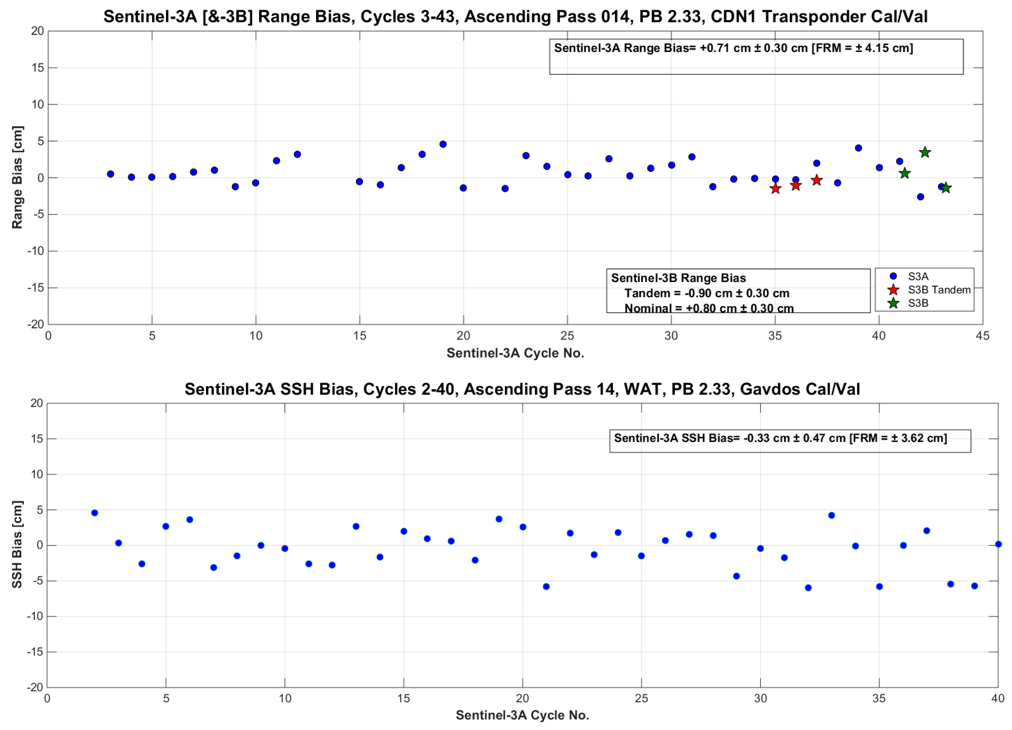
Figure 6.
Characterization and calibration procedures for the transponder to access its uncertainty at the European Space Agency (ESA) facilities in the Netherlands (The Compact Payload Test Range Facility).
Figure 6.
Characterization and calibration procedures for the transponder to access its uncertainty at the European Space Agency (ESA) facilities in the Netherlands (The Compact Payload Test Range Facility).
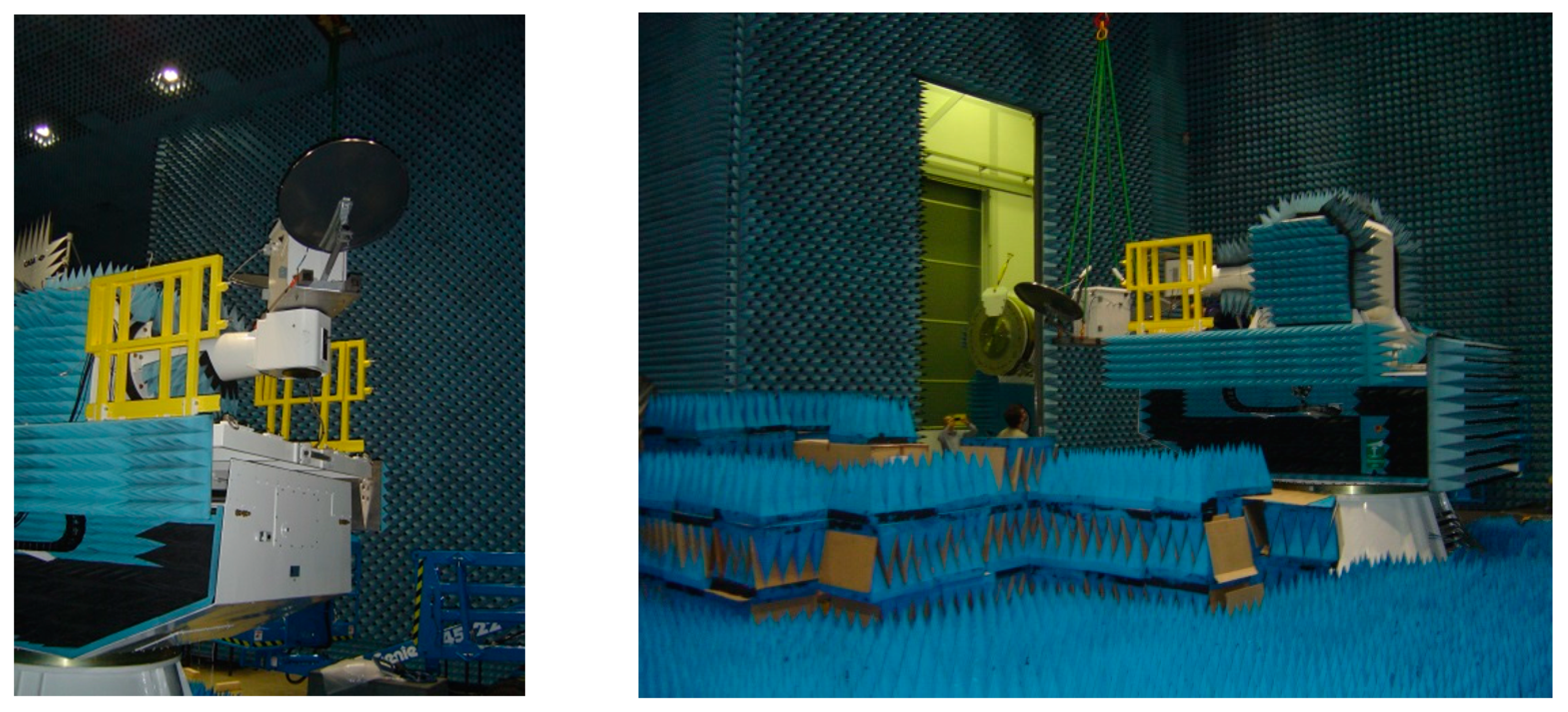
Figure 7.
The transponder and sea-surface calibrations as applied in Crete and Gavdos for the satellite altimeters.
Figure 7.
The transponder and sea-surface calibrations as applied in Crete and Gavdos for the satellite altimeters.

Figure 8.
The above diagram shows an example on how to characterize uncertainty budgets in altimetry calibration with sea-surface techniques after analyzing all the error constituents contributing in the process.
Figure 8.
The above diagram shows an example on how to characterize uncertainty budgets in altimetry calibration with sea-surface techniques after analyzing all the error constituents contributing in the process.

Figure 9.
Water level measurements by tide gauges of diverse measuring techniques are conducted at the Gavdos sea-surface Cal/Val site. The location and scale of each independent water level record is statistically evaluated independently, and a final water level value is given after an appropriate weighting of each time series.

Figure 10.
The sea-surface calibration facility in Gavdos island, south of Crete. An example with Sentinel-6/Jason-CS orbits.
Figure 10.
The sea-surface calibration facility in Gavdos island, south of Crete. An example with Sentinel-6/Jason-CS orbits.

Figure 11.
The DORIS beacon was installed in Gavdos calibration facility (above left) and collocated with a GNSS receiver (above right). The photos in the lower part of this Figure show the operating BeiDou station in the Technical University of Crete, Greece.
Figure 11.
The DORIS beacon was installed in Gavdos calibration facility (above left) and collocated with a GNSS receiver (above right). The photos in the lower part of this Figure show the operating BeiDou station in the Technical University of Crete, Greece.
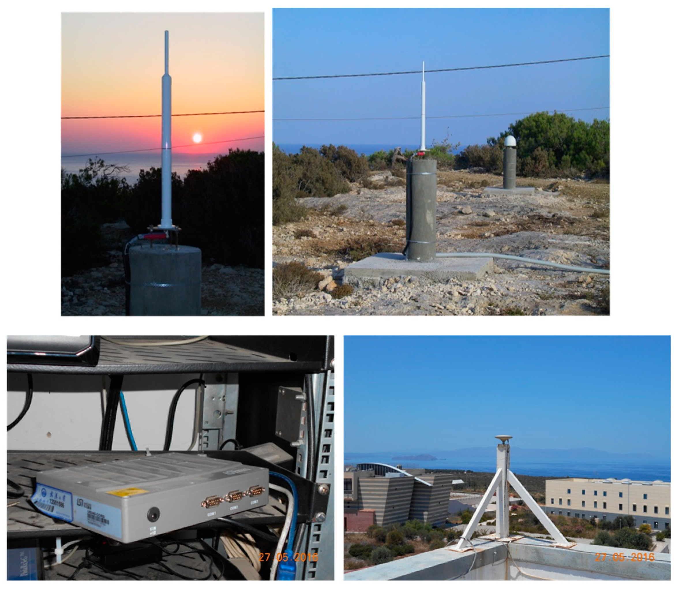
Figure 12.
The absolute robot-based GNSS antenna calibration, as carried out in Garbsten, Germany. This procedure was applied to the Leica AR25.R3 antenna operating in Gavdos Cal/Val site. The lower image shows the NOAA’s National Geodetic Survey robotic system [33,34].

Figure 13.
Upper image: The GVD8 altitude (height) daily solutions over 2014 using the IGS (“old”) and the Geo++ (“new and calibrated”) antenna parameters. Lower Image: Residuals between the two solutions in the altitude (height) determination for the GVD8 Cal/Val site.
Figure 13.
Upper image: The GVD8 altitude (height) daily solutions over 2014 using the IGS (“old”) and the Geo++ (“new and calibrated”) antenna parameters. Lower Image: Residuals between the two solutions in the altitude (height) determination for the GVD8 Cal/Val site.

Figure 14.
Relation of errors in the GPS vertical velocities with respect to length of observation (after [37]).
Figure 14.
Relation of errors in the GPS vertical velocities with respect to length of observation (after [37]).
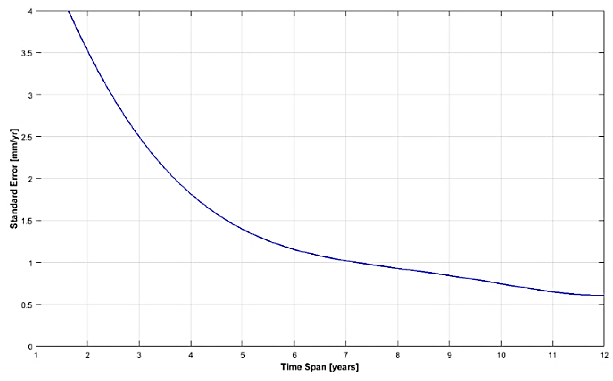
Figure 15.
The GVD8 GNSS station height and vertical velocity as derived by GAMIT and GIPSY software processing. A difference of the order of ~0.3 [mm/yr] in the vertical rate estimation is observed over 4 years of measurements.
Figure 15.
The GVD8 GNSS station height and vertical velocity as derived by GAMIT and GIPSY software processing. A difference of the order of ~0.3 [mm/yr] in the vertical rate estimation is observed over 4 years of measurements.

Figure 16.
The zero-reference measuring point of a radar tide gauge.
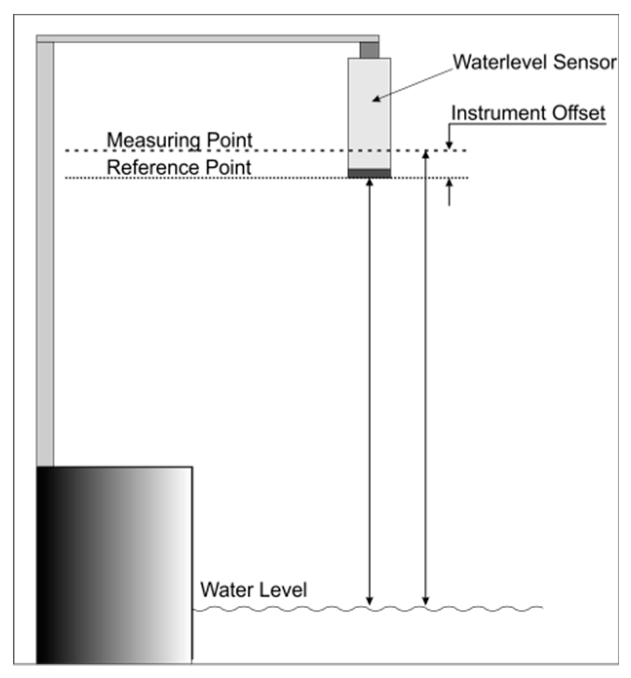
Figure 17.
Sea-surface campaigns over the satellite pass with the boat to verify the geoid and mean dynamic models in the calibrating regions of Gavdos.
Figure 17.
Sea-surface campaigns over the satellite pass with the boat to verify the geoid and mean dynamic models in the calibrating regions of Gavdos.

Figure 18.
Differences of the wet (left) and dry (right) troposphere delays as derived by GAMIT and GIPSY at the time of the Jason-3, (No. 18) overpass the CDN1 Cal/Val site.
Figure 18.
Differences of the wet (left) and dry (right) troposphere delays as derived by GAMIT and GIPSY at the time of the Jason-3, (No. 18) overpass the CDN1 Cal/Val site.

Figure 19.
The radiometer of the European Space Agency to be set up at the transponder Cal/Val site.
Figure 19.
The radiometer of the European Space Agency to be set up at the transponder Cal/Val site.

Figure 20.
The CDN1 transponder calibration site in West Crete Mountains.


Table 1.
Some examples for estimates of scale when describing uncertainty for a set of observations.
Table 1.
Some examples for estimates of scale when describing uncertainty for a set of observations.
| Scale Estimators | Statistical Definition | Remarks |
|---|---|---|
| Sample Standard Deviation | = | = sample size, observation value, sample average, |
| Trimmed Standard Deviation | = Trimming proportion, ith ordered value, = location estimate, , | |
| Mean Absolute Deviation | ||
| Median Absolute Deviation | = 0.6745 = factor for normality | |
| Fourth spread or Pseudo-sigma | are the sample 75th and 25th quantiles, are the standard Gaussian quantiles | |
| Gaussian Skip Scale | k= 2, = expected ith ordered Gaussian variables, = Biweight estimate of location, = weighting function, = Normalized deviations, c = tuning constant, S = estimate of scale (i.e., MAD) | |
| Huber’s M-estimator | , , , . | ) = first derivative of function, = scale estimate for the mth iteration, = Location estimate for the mth iteration, |
| Bi-weight A-estimators of Scale (Asymptotic Estimators) | = Median, | |
| Wave A-estimators of Scale | = Median Absolute Deviation, = Tuning constant (=2.1) | |
| Modified Wave A-estimators of Scale | = Tuning constant (=2.1) | |
| Gini’s Scale Estimator | Average of absolute differences for each pair of observations. |
Table 2.
Satellite altimeter and the on-board positioning systems along with their reference ellipsoids.
Table 2.
Satellite altimeter and the on-board positioning systems along with their reference ellipsoids.
| Altimeter | On-board Positioning System | Terrestrial Reference | Reference Ellipsoid |
|---|---|---|---|
| Jason series | GPS DORIS | WGS84 ITRF | T/P Ellipsoid |
| Sentinel-3 | GPS DORIS | WGS84 ITRF | WGS84 |
| CryoSat-2 | GPS DORIS | WGS84 ITRF | WGS84 |
| ICESat-2 | GPS | WGS84 | WGS84 |
| SARAL/AltiKa | DORIS | ITRF | T/P Ellipsoid |
| HY-2A | GPS DORIS | WGS84 ITRF | T/P Ellipsoid |
Table 3.
Examples of how uncertainties should be calculated following the fiducial reference measurements strategy and the guide for expressing uncertainties. The left table refers to sea-surface calibration and the right table corresponds to transponder calibration. The final standardized uncertainty (at 68% confidence level) based on a sea-surface Cal/Val procedure, described in terms of a Root-Sum-Square value, has been computed as for example, for the left three columns of table as .
| Cal/Val Constituent (Sea Surface) | Uncertainty Estimate | Standard Uncertainty (Confidence 68%) | Cal/Val Constituent (Transponder) | Uncertainty Estimate | Standard Uncertainty (Confidence 68%) |
|---|---|---|---|---|---|
| GNSS Height | 0.11 mm | ± 0.11 mm | Measured Range | 3.00 mm | ± 1.73 mm |
| GNSS Receiver | 6.00 mm | ± 3.46 mm | Transponder Internal Delay | 30.00 mm | ± 15.00 mm |
| GNSS Antenna Reference Point | 2.00 mm | ± 2.00 mm | Dry Tropospheric Delay | 2.00 mm | ± 1.15 mm |
| Water Level | 1.30 mm | ± 1.30 mm | Wet Tropospheric Delay | 14 mm | ± 8.08 mm |
| Tide-Gauge Zero Reference | 0.15 mm | ± 0.15 mm | Ionospheric Delay | 4.00 mm | ± 2.31 mm |
| Tide-Gauge Vertical Alignment | 2.40 mm | ± 1.39 mm | Geophysical Corrections | 20.00 mm | ± 11.55 mm |
| Tide-Gauge Sensor Certificate | 5.50 mm | ± 5.50 mm | Satellite Orbit Height | 50.00 mm | ± 28.87 mm |
| Leveling | 0.11 mm | ± 0.11 mm | Pseudo-Doppler Correction | 2.00 mm | ± 2.00 mm |
| Monumentation | 1.10 mm | ± 0.64 mm | GNSS Instrument | 6.00 mm | ± 3.46 mm |
| Vertical Misalignment | 1.00 mm | ± 0.60 mm | GNSS Antenna Reference Point | 2.00 mm | ± 2.00 mm |
| Leveling Observer | 1.00 mm | ± 0.60 mm | GNSS Repeatability | 0.14 mm | ± 0.14 mm |
| Leveling Instrument/Method | 1.00 mm | ± 0.60 mm | Transponder Leveling | 0.16 mm | ± 0.16 mm |
| Tide Pole Reading During Calibration | 1.00 mm | ± 0.60 mm | Leveling Instrument/Method | 1.00 mm | ± 1.00 mm |
| Mean Sea Surface (Mean Dynamic Topography and Geoid) | 33.0 mm | ± 33.00 mm | Processing and Approximations | 30.00 mm | ± 17.32 mm |
| Processing and Approximations | 0.5 mm | ± 0.29 mm | Orbit Interpolations | 0.30 mm | ± 0.17 mm |
| Geoid Slope | 10.0 mm | ± 5.77 mm | Unaccounted Effects | 20.00 mm | ± 11.55 mm |
| Unaccounted Effects | 20.0 mm | ± 11.55 mm | |||
| Root-Sum-Squared Uncertainty | ± 36.16 mm | Root-Sum-Squared Uncertainty | ± 41.49 mm |
© 2019 by the authors. Licensee MDPI, Basel, Switzerland. This article is an open access article distributed under the terms and conditions of the Creative Commons Attribution (CC BY) license (http://creativecommons.org/licenses/by/4.0/).
Share and Cite
MDPI and ACS Style
Mertikas, S.P.; Donlon, C.; Vuilleumier, P.; Cullen, R.; Féménias, P.; Tripolitsiotis, A. An Action Plan Towards Fiducial Reference Measurements for Satellite Altimetry. Remote Sens. 2019, 11, 1993. https://doi.org/10.3390/rs11171993
AMA Style
Mertikas SP, Donlon C, Vuilleumier P, Cullen R, Féménias P, Tripolitsiotis A. An Action Plan Towards Fiducial Reference Measurements for Satellite Altimetry. Remote Sensing. 2019; 11(17):1993. https://doi.org/10.3390/rs11171993
Chicago/Turabian StyleMertikas, Stelios P., Craig Donlon, Pierrik Vuilleumier, Robert Cullen, Pierre Féménias, and Achilles Tripolitsiotis. 2019. "An Action Plan Towards Fiducial Reference Measurements for Satellite Altimetry" Remote Sensing 11, no. 17: 1993. https://doi.org/10.3390/rs11171993
Note that from the first issue of 2016, this journal uses article numbers instead of page numbers. See further details here.