Bringing Lunar LiDAR Back Down to Earth: Mapping Our Industrial Heritage through Deep Transfer Learning


Camborne School of Mines, University of Exeter, Tremough Campus, Penryn TR10 9EZ, UK
*
Author to whom correspondence should be addressed.
Remote Sens. 2019, 11(17), 1994; https://doi.org/10.3390/rs11171994
Submission received: 31 July 2019
/
Revised: 15 August 2019
/
Accepted: 21 August 2019
/
Published: 23 August 2019
(This article belongs to the Special Issue Archaeological Remote Sensing in the 21st Century: (Re)Defining Practice and Theory)
Abstract
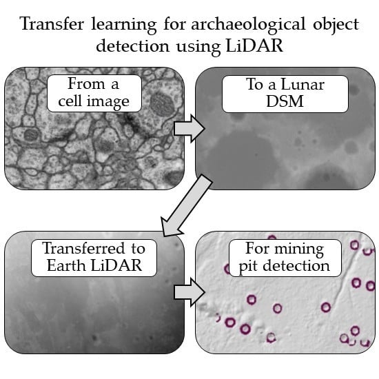
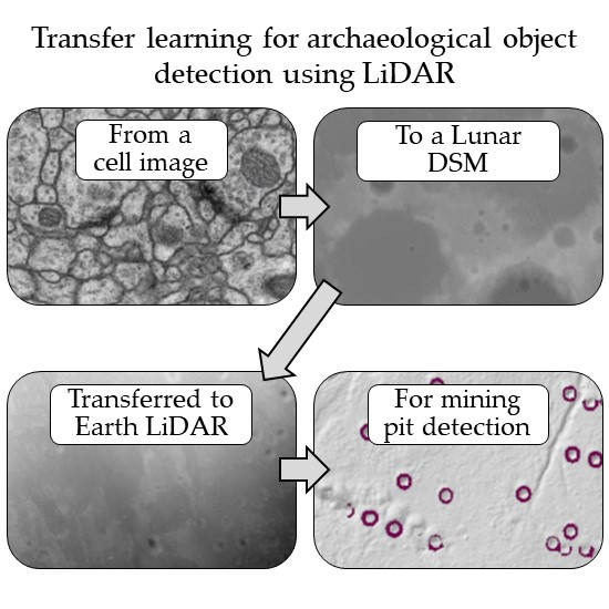
:This article presents a novel deep learning method for semi-automated detection of historic mining pits using aerial LiDAR data. The recent emergence of national scale remotely sensed datasets has created the potential to greatly increase the rate of analysis and recording of cultural heritage sites. However, the time and resources required to process these datasets in traditional desktop surveys presents a near insurmountable challenge. The use of artificial intelligence to carry out preliminary processing of vast areas could enable experts to prioritize their prospection focus; however, success so far has been hindered by the lack of large training datasets in this field. This study develops an innovative transfer learning approach, utilizing a deep convolutional neural network initially trained on Lunar LiDAR datasets and reapplied here in an archaeological context. Recall rates of 80% and 83% were obtained on the 0.5 m and 0.25 m resolution datasets respectively, with false positive rates maintained below 20%. These results are state of the art and demonstrate that this model is an efficient, effective tool for semi-automated object detection for this type of archaeological objects. Further tests indicated strong potential for detection of other types of archaeological objects when trained accordingly.
1. Introduction
Airborne LiDAR systems are an increasingly valuable tool for locating, visualizing and understanding cultural heritage sites. The ability to perceive subtle depressions and patterns in the landscape uncoupled from photometric representations has led to discoveries ranging from additional monuments at Stonehenge [1] to Mayan cave dwelling entrances in Belize [2]. These are examples of the more traditional uses of LiDAR in archaeology, where data over a small area is visually analyzed through an experience and knowledge based process to obtain a detailed understanding of a landscape, usually by displaying the LiDAR data as a hillshaded image [3]. This approach is effective for discrete areas, especially where high resolution datasets have been gathered, but does not fully leverage the advantages of newly available large scale general purpose LiDAR datasets [4]. Whilst analysis by experts will always produce the best results, the increasing availability of these new datasets now requires a paradigm change towards the integration of computer aided detection to take advantage of these greatly increased volumes of data [5].
In England alone, the Environment Agency has pledged nationwide coverage at 1 m resolution or higher by 2020, totaling over 130,000 km2 of coverage [6]. Scotland has currently been partially covered by a two phase campaign, with more coverage planned for the future [4]. Analyzing these volumes of data efficiently by human operators is extremely challenging. For example, the English Heritage National Mapping Program (primarily aerial image interpretation) achieves a coverage rate of approximately 1 km2 per person per day; this project has been running for over 20 years employing on average 15–20 staff and had covered an area of 52,000 km2 by 2012, in contrast, the Baden-Württemberg study, whilst still a primarily manual approach, took advantage of automated processing where possible, allowing an estimated coverage rate of over 35,000 km2 by a single operator in six years [7]. These two projects are not directly comparable, as the quality and accuracy of their results varies greatly along with the data types analyzed [3], but it is an indication of the speed advantages gained from integrating automated processes into an analysis workflow. Despite the differing data types, the English Heritage study provides an indication of the timescales required to put human eyes over nationwide remotely sensed data tiles at a high resolution scale. With current advances in computing power the potential to pre-process entire national datasets in weeks rather than decades is now a distinct possibility.
This approach would be particularly valuable for countries which do not have many existing historic site records; a rapid Artificial Intelligence (AI) scan would provide a preliminary database which could be developed further as more resources become available. Due to the very low time and cost overheads required for automated processing there can be complementarity between achieving the quantity of the automated results versus the quality of traditionally generated databases, which can proceed to be created as normal in tandem to the automated processing. Even if imprecise, these machine learning tools would be capable of identifying the greater trends in the data [3], allowing human resources to be prioritized to the areas with a large number of potential sites for detailed precision mapping. Especially when sites are under threat from development, rapid identification and mapping would give cultural heritage managers more time to act.
In the UK, sites such as those defined by English Heritage as National Importance sites would also benefit from a semi-automated approach. These are sites that are deemed to have national importance but are not currently or cannot be designated as heritage assets and scheduled monuments [8]. Many of these sites have a landscape scale, consisting of ‘a coherent and contiguous group of monuments, the group value of which augments the significance or importance of each, though the importance of the whole landscape can also be defined in its own terms’ [8]. Identification and delineation of sites such as these remains a challenge due to limited mapping resources and the large extent of these sites. Large-scale monument counting tools, especially if cheap and efficient to run, would underpin more informed management of these types of sites, provided the sites present above ground topographical representations visible to an aerial LiDAR sensor. The results from such a preliminary survey could be stored in a geospatial database such as that described in [9].
Alongside the vast speed improvements possible from semi-automated detection, computer-based methods have other strengths compared to human observers. Humans are inherently unable to process height data in its native state; therefore, it must be processed to create visualizations that are interpretable by the human eye. This can lead to a loss of information, image artefacts [10] or a bias stemming from the visualization techniques used [11]. As a computer can process the single channel numeric gridded height data directly, this removes some of these issues. Conversely, multi-channel or hyperspectral data containing more than three channels is also not easily representable in a human readable form [12], whereas a computer can stack as many channels as necessary to process hyperspectral or multiple data source imagery. Artificial intelligence based solutions can also make their own generalizations and assumptions; often different to those that a human would make. Whilst this in itself will create biases, discussed later in this work, the addition of a very alien ‘brain’ to the problem will go some way to alleviate human biases. Humans see what they are expecting to see [13], and a trained neural network will also see what it is expecting to see; using both allows for potentially unexpected objects to be discovered.
However, despite all the advantages discussed above, computer aided methods are still inferior to human interpretation in terms of accuracy, inference and knowledge [3]. To benefit from the power of automation whilst maintaining the experience and insight gained from human experts a twofold approach is needed. The challenge lies in both improving the algorithms to a point where they are ‘fit for purpose’ and integrating the semi-automated detections into the archaeological prospection workflow in an appropriate manner [3]. It is envisioned that once applicable tools have been designed, they would be run as a pre-processing step over entire datasets, narrowing the areas to be inspected manually. Another integration possibility is the combined citizen science and automation workflow proposed in [14]. The integration of citizen science is already a powerful and well developed methodology for both conventional and semi-automated LiDAR projects addressing the need for more manpower than is available from experts in the field, alongside leveraging the intimate knowledge of a local area provided by the people who live, work and recreate there [15,16]. However, a major building block of any large-scale site detection system is the algorithm itself; accurate, generalizable and repeatable methods are required to create confidence in such a system and much research has been focused on this problem.
Early methods for semi-automated archaeological site identification used template matching (where a predefined template is passed over the scene) or rule-based methods (where rules are applied to determine an object’s category). Successful applications of template matching are described by Trier in [17,18]. Other proposed methods utilize Geographic Object-Based Image Analysis (GEOBIA), examples of these are described in Sevara et al. [19] and Freeland et al. [20]. These types of techniques require prior knowledge of the shape and size of the object to be identified and perform well on relatively simple geometries but are less effective at generalizing to unseen or partially occluded examples [21]. This is because these methods are responding to preprogramed definitions of the object to be detected rather than ‘taught’ about the object features.
Machine learning is where a computer model is developed that can recognize features. The model is developed by ‘training’—a process by which known examples are fed into the model and it is adjusted until it can predict the correct answer. The model is then evaluated with a second set of known examples (to ensure that the model does not simply memorize the data) before being used in a real situation. There are many types of machine learning algorithms from simple statistical models to deep neural networks. Recently, some results with very high accuracy have been obtained by combining an advanced visualization technique based on topographic deviation at multiple scales with a random forest machine learning classifier to identify Neolithic burial mounds [22].
In the field of computer vision, a particular type of neural network called a convolutional neural network (CNN) has been shown to be capable of solving diverse and complex problems such as visual image question answering [23] and real time object detection for over 9000 categories [24]. Considerable research has been carried out in the broader remote sensing community as to how to design and modify similar systems for aerial remote sensing tasks. Primarily this work has involved Very High Resolution (VHR) images as the input to the CNN, either building their own network architecture [25] or modifying and fine tuning existing computer vision models [26,27]. Nogueira et al. [28] give an overview of the advantages and disadvantages of these approaches, concluding that fine tuning an existing trained model provides the best results, however, the lack of an appropriate training datasets makes it very difficult to develop a model. Borrowing a similar model and transferring it to the problem at hand is one possible solution [29].
The primary balance that must be addressed when choosing an approach is the applicability of the model versus the availability of training data. If training data and computing power allow, the ideal scenario is to design and train a model from scratch for the required task using the specific data that is required. However, available training datasets for remote sensing data are small and usually not representative of a wide range of environments. Conversely, labelled training datasets in the computer vision community are vast: ImageNet has over 14 million labelled images in 20,000 object categories [30] and models trained on these large datasets tend to be less prone to overfitting and can generalize well compared to ones trained on small datasets [28]. However, there are differences in the type of objects they have been trained to detect. For example, in computer vision the objects tend to take up more of the frame and can appear at very different scales, but generally not in many different rotations, whereas for aerial data the scale is relatively constant, but the object can have many rotations [27]. When using a pretrained model to generalize to images created from a LiDAR DEM the problem is exacerbated, as most existing models have been trained on three channel RGB images and not one channel depth images. This, along with the differing ways that objects appear in a LiDAR DEM versus imagery, can make transfer learning with LiDAR data challenging [31].
Two published studies have used CNNs with LiDAR data to identify archaeological objects, with promising results. Trier et al. [32] found strong positive identifications on one dataset but on their second dataset, which contained more varied objects, their results were less conclusive. Verschoof-van der Vaart and Lambers [33] employed a similar methodology using variously trained versions of the same pretrained deep learning model to detect multiple classes of archaeological objects, achieving accuracy scores comparable or surpassing those obtained by the other machine learning methods. In both studies a transfer learning technique was used, with the essential methodology involving the generation of a local relief model [34] from the LiDAR data and then either converting this generated single channel image into a conventional three channel image stack by triplicating the greyscale channel [32] or by modifying the input layer of the CNN [33]. Both studies used models that had been trained on RGB images of terrestrial scenes such as ImageNet. A recommendation from both studies was to use a model pretrained on data more similar to LiDAR data in the future; however, obtaining such models was determined to be challenging.
A possible solution can be found in the planetary remote sensing field. Large planet scale digital DEM datasets exist from sources such as the Lunar Reconnaissance Orbiter [35] and the Mars Global Surveyor [36]. Several studies have built and trained CNNs to detect craters from these datasets [37,38,39]. These models are designed to be highly receptive to elevation changes and to roughly circular patterns observed in single channel DEM images. This makes them a good fit for the problem of archaeological object detection. An example of this type of model was built by Silburt et al. [37], based on the U-net semantic segmentation model, itself originally designed for medical image segmentation [40]. This model, named DeepMoon (Available at https://github.com/silburt/DeepMoon.git) was trained on 30,000 labelled images randomly extracted over the entire surface of the moon combined with the existing catalogues of moon craters. This is a larger and more robust training data set than those available for archaeological remote sensing, solving the problem of applicable transfer learning datasets.
In this paper we propose a highly effective transfer learning strategy to detect historic mining pits utilizing the DeepMoon base model fine-tuned with local LiDAR data. Several different resolutions and representations of LiDAR data are tested, and the final model predictions are verified with a full ground inspection. Mining remains were chosen as the class of interest as there is a rich mining cultural history in South West England, and the evidence of these historic extractive industries is both numerous and well recorded. These mining areas are also suitably covered by freely available high-resolution LiDAR data. Whilst this model has been trained and tested specifically to detect historic mining pits, it is hypothesized that the principals will remain true for any archaeological feature that presents with a circular height change in aerial LiDAR data, such as: Charcoal kilns [41], pitfall traps [42], shell rings [43], conical mounds [18,20,43] and roundhouses [32] Thus, our method has potential applicability across many archaeological prospection challenges when furnished with appropriate training data.
2. Materials and Methods
2.1. Study Area
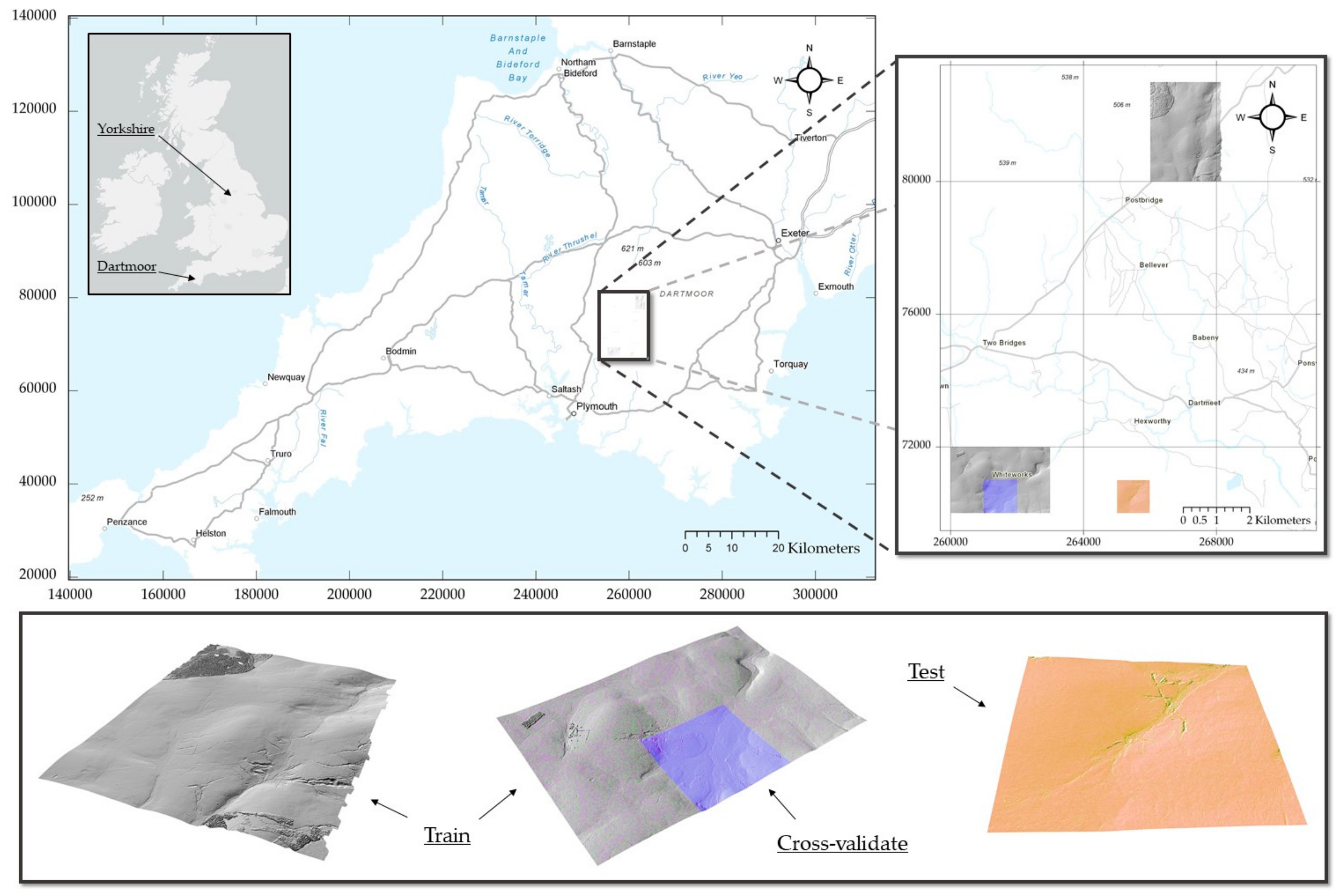
The primary study area for this research is Dartmoor National Park, an upland area of moorland studded with exposed granite hilltops known as tors. The ground cover is primarily low vegetation, including heather, bracken, gorse, fern and marsh grasses. Tin and copper mining on Dartmoor has taken place almost continuously from the 12th to the 20th centuries and the remains are pervasive and visually striking throughout the landscape [44]. Three areas of concentrated historic mining activity were used to develop this deep learning model; these are shown in Figure 1. The different colors in Figure 1 refer to the distribution of training, validation and testing data. The training and validation areas include in the north the old Birch Tor Mine (1726–1928) [45] and in the south the former Whiteworks Mine. It is believed that the Whiteworks area was being mined as early as 1180 although the mine was expanded substantially around 1790 towards the beginning of the industrial revolution when the demand for tin increased [45]. The mine was owned by the wealthy Tavistock mining entrepreneur Moses Bawden and operated for just under 100 years until 1880, briefly reopening in early 1900 before finally closing for good by 1914 [46]. The test area for Dartmoor is the site of Hexworthy Mine (1891–1912). This is an interesting site as it displays remains from multiple eras of mining; from the early unrecorded open workings, through traditional 19th century mining to semi-modern 20th century workings [47]. The mine operated productively until the call up for men in 1914, during the war it was placed in care and maintenance before a large storm in 1920 destroyed the waterwheel flume, causing the underground workings to flood [46].
A further testing area was selected in the Yorkshire Dales National Park more than 500 km from Dartmoor to examine the model’s ability to generalize to new locations, mine types and data resolutions. This test area is part of the site of the former Grassington Moor lead mine. The first known exploitation of lead at Grassington was by the 4th Earl of Cumberland in the early 17th century, although it is thought that some primitive extraction and smelting had taken place earlier. The early exploitation involved the digging of shallow shafts along the vein. The first mill to process the Grassington lead ore was the Low Mill built in 1605. The test area covers the western part of the Yarnbury mine, including Tomkins, Barretts and Good Hope shafts [48].
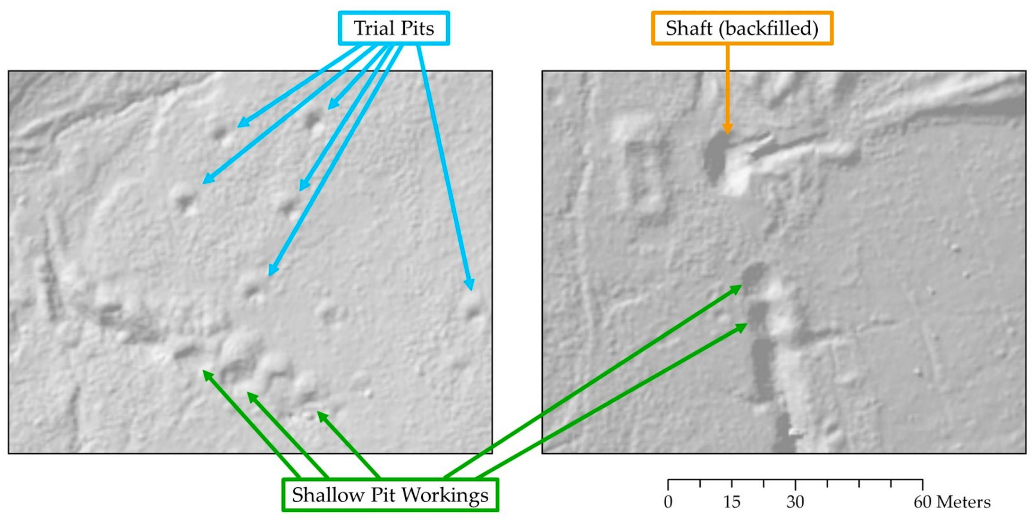
In all cases, the objects to be detected are trial pits, shallow pit workings and shaft heads. Examples of these are shown in Figure 2. Trial pits are dug whilst prospecting for tin lodes. They are usually 2–3 m in diameter, of limited depth (up to 1 m) and are often silted, water filled and reedy [44]. Shallow pit workings are comprised of alignments of deeper pits which are dug to below the soil overburden and mined downwards from there; however, these are not underground mines and there is no lateral development between the pits. The depth of these types of workings would be limited by the ability of the surrounding side-walls to remain intact before collapsing, which is usually less than 3 m. These workings present as conical depressions often accompanied by a ring of spoil material, crescentic on the downhill side in sloping ground [44]. The final category are shafts for true underground mines. These have mainly been capped or backfilled in Dartmoor for public safety; however, evidence may remain in the form of large conical pits or straight openings. Site inspections may reveal a collar of finished material lining the inside of the shaft, but this is generally not visible from aerial surveys.
2.2. Data Pre-Processing
The LiDAR datasets used for this project was obtained from the Environment Agency under their Open Government License and are available at https://environment.data.gov.uk/ [49]. The Dartmoor data was flown in 2009 at a resolution of 0.5 m and the Yorkshire data in 2012 at a resolution of 0.25 m. In total twelve 1km × 1km tiles were processed for this study. Both datasets are available in either Digital Surface Model (DSM) or Digital Terrain Model (DTM) formats produced by the Environment Agency. The DSM was chosen in preference to the filtered DTM due to concerns that the filtering algorithms used to produce the DTM can excessively smooth small features [50].
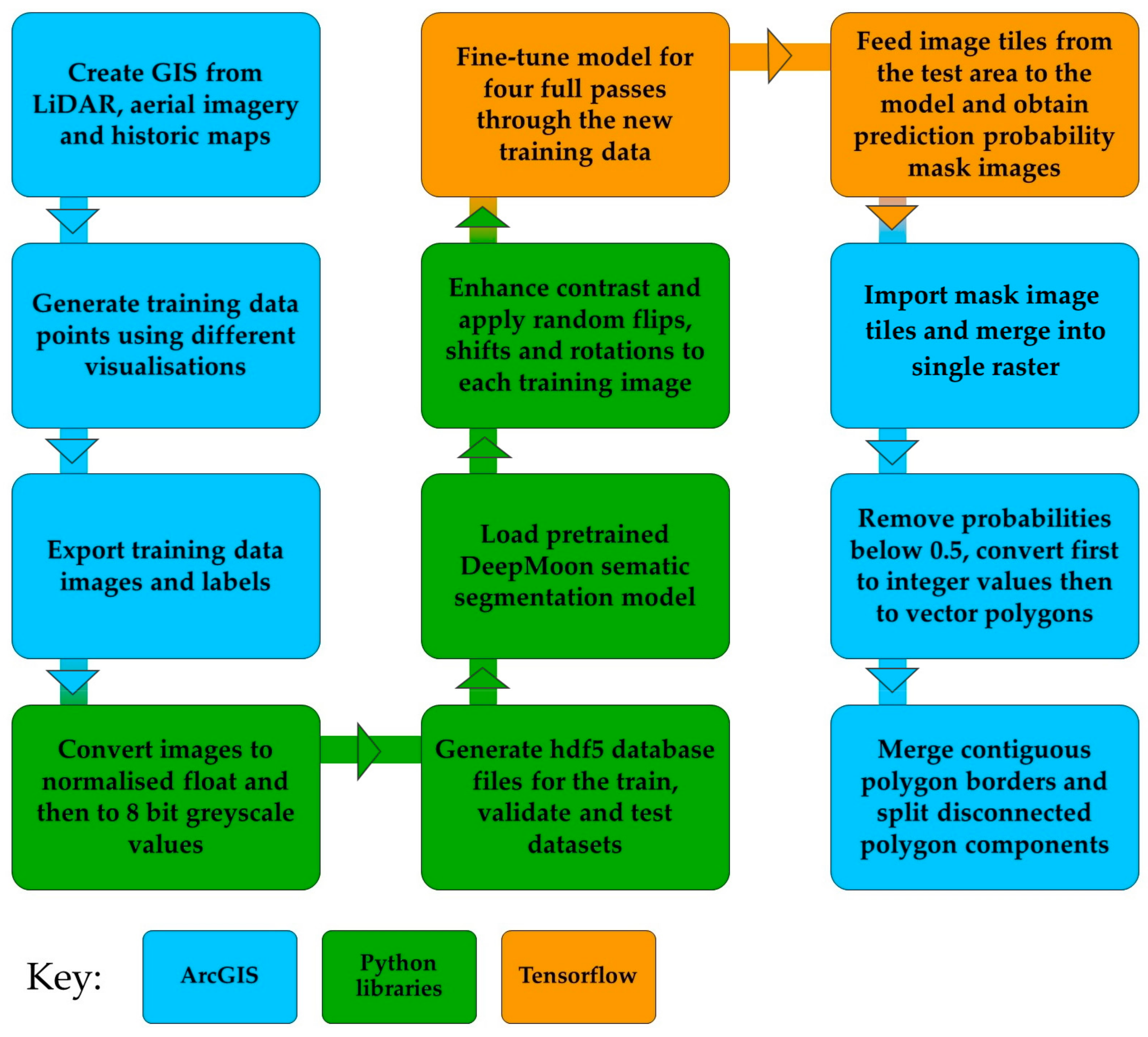
The data was imported into ArcGIS Pro [51] along with several other interpretive layers such as historical maps [52] and aerial images [53] to create a GIS of the study area. Other GIS software could be used for this step, but ArcGIS Pro was chosen as it has a function for automatic exporting of image tiles and training labels, crucial for the later steps of the workflow. The additional GIS layers were only used to add context to the dataset to aid the human operator. To generate training and validation datasets, a desktop survey was carried out to identify features resembling mining pits. From this survey over 1,500 samples were identified and marked as point features. The test area dataset was created in the same way, but in order to validate the performance of the model every feature in the test set was also confirmed with a ground survey. This survey involved visiting the test sites with two reference maps, one containing the predictions and one containing the human generated pit locations from the desktop survey. Using these maps in conjunction with a handheld GPS for site orientation the true existence of pits shown on the maps was confirmed or rejected. The pits were not recorded with the GPS as in many cases it is not safe to access the ground directly above suspected shafts. A schematic of the project process is shown in Figure 3 and full details of the processing steps are provided in Supplementary Document S1.
For the model inputs, image tiles of 256 × 256 pixels were exported along with the pit locations as xml labels to create image segmentation masks. The overlap between tiles was set to 52%. To preserve the fine detail in the DSM image, the image tiles first were exported as 16-bit float images with the values corresponding to the actual ground elevation of the data within that tile. Each tile was then individually rescaled to greyscale values between 0–1 maintaining its original distribution before finally being converted to an 8-bit integer format. To enhance contrast the image tiles were further rescaled linearly prior to model input. The image tile preparation process is shown in Figure 4. For the training and validation datasets, only image tiles which contain mining pits were exported. The training dataset contains 520 images and the test and validation datasets contain 70 images each. These datasets are stored in hdf5 format with the image names used as the database key. Table 1 shows the dataset split, number of pits and pit instances per dataset, along with the minimum, mean and maximum pits per image tile. The pit instances are greater than the number of pits as some pits are present on more than one image tile due to the >50% overlap between tiles.
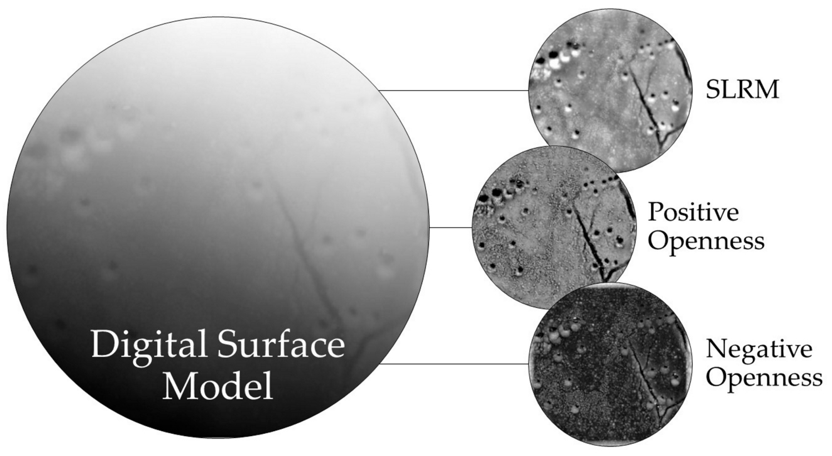
Other visualization of LiDAR data have been shown to aid in identification of archaeological features. Using the Relief Visualization Toolbox [10,54] several other representations of the data were generated from the original exported tiles. A simplified local relief model (SLRM) is a representation where the major features of the landscape have been removed. This process is known as detrending. These models are created first by smoothing a DEM so that small features are removed. The smoothed DEM is then compared to the original DEM and areas that are the same in both models are extracted to build the new smoothed DEM. This is finally subtracted from the original to produce the SLRM [34]. The SLRM is a very clear way to depict small relative changes in the landscape such as those from archaeological or mining features, and is the visualization method chosen by both [32,33] for their models.
Alongside the SLRM another visualization type known as openness was created. Openness is a geographical visualization technique that is calculated by measuring the angular size of a sphere either looking up or down from each pixel. It is described as either positive or negative openness. Negative openness is not the inverse of positive openness and highlights deep features instead of protruding features. As openness is calculated in relation to terrain rather than the sky, features on slopes appear the same as features on horizontal ground [55]. This is a valuable property for the Dartmoor data as most of the features are situated in rolling moorland terrain. Figure 5 illustrates the different visualization types generated for this study.
2.3. Deep Learning Model
The type of model used in this research is a variant of an Artificial Neural Network (ANN) known as a Convolutional Neural Network (CNN). A simple ANN contains one or more hidden layers, with every node in a hidden layer directly connected to every node in the layers before and after it. Each node has a weight associated with it which determines the final output result. When first initialized, the weights are randomly assigned and the first result from the network most likely will be incorrect. The direction in which to change the weights to approach the correct answer is then determined using gradient descent and the weights are updated; this process is known as backpropagation. The network continues to feedforward and backpropagate until it has converged on a satisfactory result. Each input is treated individually, therefore a 256 × 256 pixel image would have 65,536 inputs; as input images get larger the process becomes untenable.
The original Convolutional Neural Network was proposed by Lecun et al. [56], however the power of CNNs to solve complex image processing problems was not capable of being fully realized until the advent of powerful graphical processing units since 2010, with the first highly successful implementation [57] winning the 2012 Large-Scale Visual Recognition Challenge (ILSVRC) by a significant margin. CNNs improve upon the ANN design by allowing the sharing of weights across nodes, thus greatly decreasing the number of weights to optimize whilst also introducing spatial connectivity across the image. This is achieved by convolving a filter across the image which activates different underlying structures. The result of this convolution is a feature map. A single convolutional layer can have many filters, producing a multidimensional feature map of activations. To reduce the dimensionality of the image and increase the field of view of the filter, downsampling via max pooling is carried out on the layers to reduce the spatial dimensions. For a detailed description of the theory and mathematics of CNNs, see [58] Chapter 9.
In general, the lower layers of a CNN have high spatial resolution and describe the low level features which make up an image, and the upper layers have low spatial resolution and describe more complex patterns such as objects. For the task of image classification this is the final convolutional stage, as the question being asked is whether a certain object is present in the image. The next step, object detection is popularly achieved using R-CNNs, which use a region proposal network to identify areas of the image which may contain objects, these regions are then extracted and classified [59]. Finally, semantic segmentation, where every pixel in the image is assigned a class can be achieved by either extending the R-CNN approach [60] or by adding a deconvolutional network which up-samples the high level, low resolution feature layers by up-convolution to return to the resolution of the input image; this architecture is known as an encoder-decoder model [40].
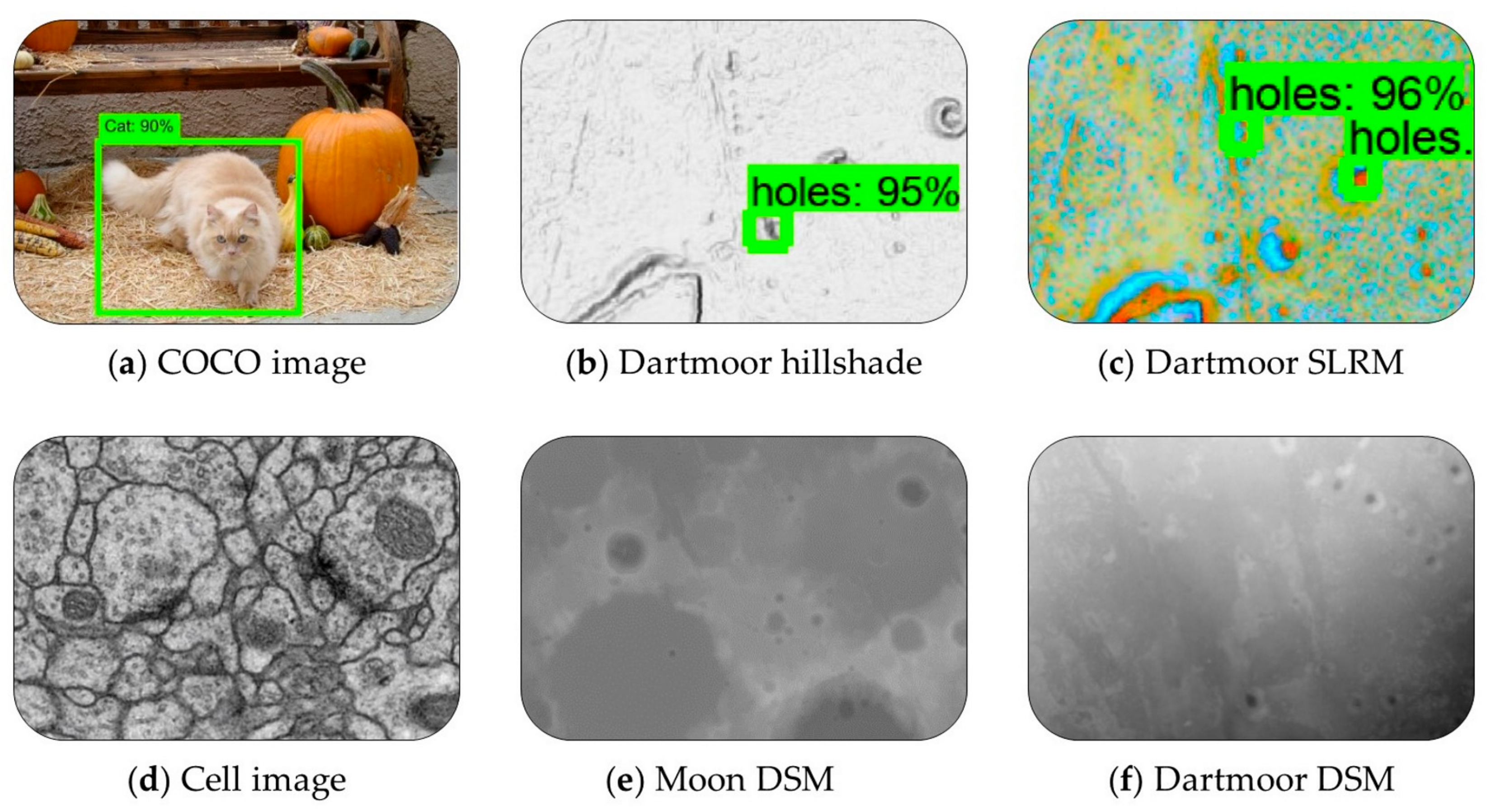
Initially in this research an object detection pipeline using the Inception model [61] pretrained on the Common Objects in Context dataset [62] was trialed. The preliminary results from this method were reasonable but there appeared to be many mining pits not detected by the model even after 100,000 training epochs. Images from this initial method are shown in Figure 6. It is suspected that the mining pits detection task is simply too different from the original task to achieve optimum results. These initial tests showed a detection rate of less than 40%, this result, along with the recommendations from Trier et al. [32] motivated a search for a transfer learning candidate model that resembles more closely the task at hand instead of continuing to refine the Inception model.
After exploring several alternatives, the exact model chosen for this study is a version of the U-net model designed by Ronneberger et al. [40] and modified by Silburt et al. [37]. The U-net model is an encoder-decoder (see [63]) model with a near symmetrical architecture, designed for biomedical image segmentation. It has no final fully connected layer, replacing it with a 1 × 1 convolutional layer with a sigmoidal activation function to output pixelwise class probabilities, thus reducing the number of hyperparameters to tune and making it more suitable for small numbers of training data. The original U-net achieved significant accuracy improvements over the next best architecture in the ISBI cell tracking challenge despite the training set only containing 35 images [40]. Biomedical image analysis shares many challenges with remote sensing LiDAR analysis such as small training sample sizes, single channel images and high resolution data. Therefore, it is more applicable to use a model such as U-net rather than one of the models designed for large datasets of natural images, as shown in Figure 6.
2.4. Transfer Learning
Nogueira et al. [28] found that for remote sensing problems with limited training data, a transfer learning strategy achieved the most accurate results across all tested datasets. In transfer learning, instead of initializing the model weights from scratch, the weights from another model trained for many epochs on a larger dataset are used. One transfer learning strategy involves removing the last layer of the network and replacing it with a layer to classify the objects of interest, this is required if the final classification categories are different. Another approach is to fine tune a model by adding new training examples whilst keeping the final output layer the same. All the model weights can be updated, or the lower layers can be frozen and only the weights in the upper layers are updated. For this research, as the classification is the same geometrically if ‘crater’ is substituted for ‘pit’ a fine-tuning strategy was employed with all weights unfrozen and the learning rate set to 10−4. As this study utilizes a pre-existing model, the same software (Python [64], TensorFlow [65] and Keras [66]) used by the creators of the original DeepMoon model [37] are used throughout. All of these packages are industry standard and available free from their respective websites.
2.5. Training
In a neural network the hyperparameters can be used to control overfitting; for the DeepMoon model, the hyperparameters include weight regularization for the convolutional layers, dropout layers, filter size, model depth, and learning rate. Full details on these hyperparameters and complete model design can be found in [37]. These hyperparameters were chosen after a cross validation check using 60 models, where the hyperparameters were chosen randomly from across their standard ranges. To avoid overfitting on the small project dataset used in this research the hyperparameters chosen in [37] have been maintained here, with only minimal fine tuning training. Silbert’s base model was trained for 4 epochs (where one epoch equals a full pass through the entire training set). As the lunar dataset contained 30,000 images this training totaled 120,000 training examples. A standard learning rate of 10−4 was found to deliver the best results [37]. The additional training for transferring the model to its terrestrial archaeological context involved 4 more epochs of 520 images, totaling 2080 new training examples. The number of fine-tuning epochs was varied to determine the most effective fine-tuning strategy, this is discussed further in Section 3.1. To further control overfitting between epochs data augmentation is carried out, where all input images are randomly flipped, rotated and shifted prior to model input.
2.6. Post-Processing
Once the model is trained and verified against the cross validation dataset, individual image tiles to be tested are inputted to the model and probability masks are outputted as tif files. Using the same naming convention for both input and output files results in correct translation into the original coordinate system. Using ArcGIS, all output probability masks are then mosaiced into one continuous raster covering the entire test area.
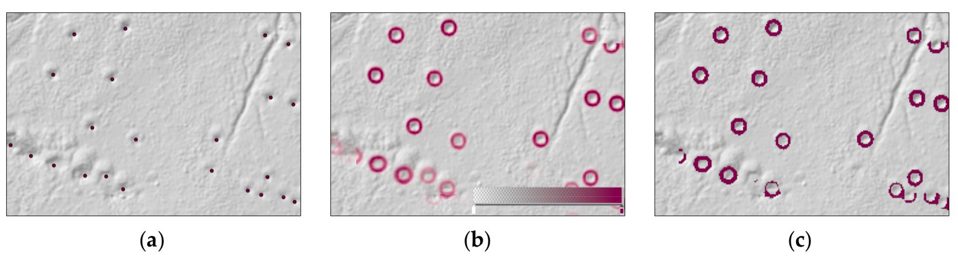
For qualitative visual analysis and map creation, a graduated stretch symbology where solid color depicts probabilities of 1 and fully transparent depicts probabilities of 0 is used for maximum readability. This visualization scheme maintains information on the confidence of the prediction and allows for the more subtle workings of the model to remain visible. This enhances the model’s readability in comparison to a yes/no response as it symbolizes uncertainty in the model, allowing an archaeological prospector more freedom to interpret the results using superior human reasoning. To quantitatively determine the rate of true positives, false negatives and false positives in order to report accuracy metrics, a new binary mask layer was created containing only pixels with prediction probabilities above 0.5. These pixels were then vectorized, merged and filled to create a vector layer of predicted pits to use in spatial queries. A comparison of these post processing methods is shown in Figure 7. It can be seen in Figure 7c that there are some incomplete rings, this is because some detections are made up of a mixture of pixels above and below 0.4 probability. This further supports the decision to use the full masks rather than the instances for interpretation where possible.
3. Results
3.1. Cross Validation Results
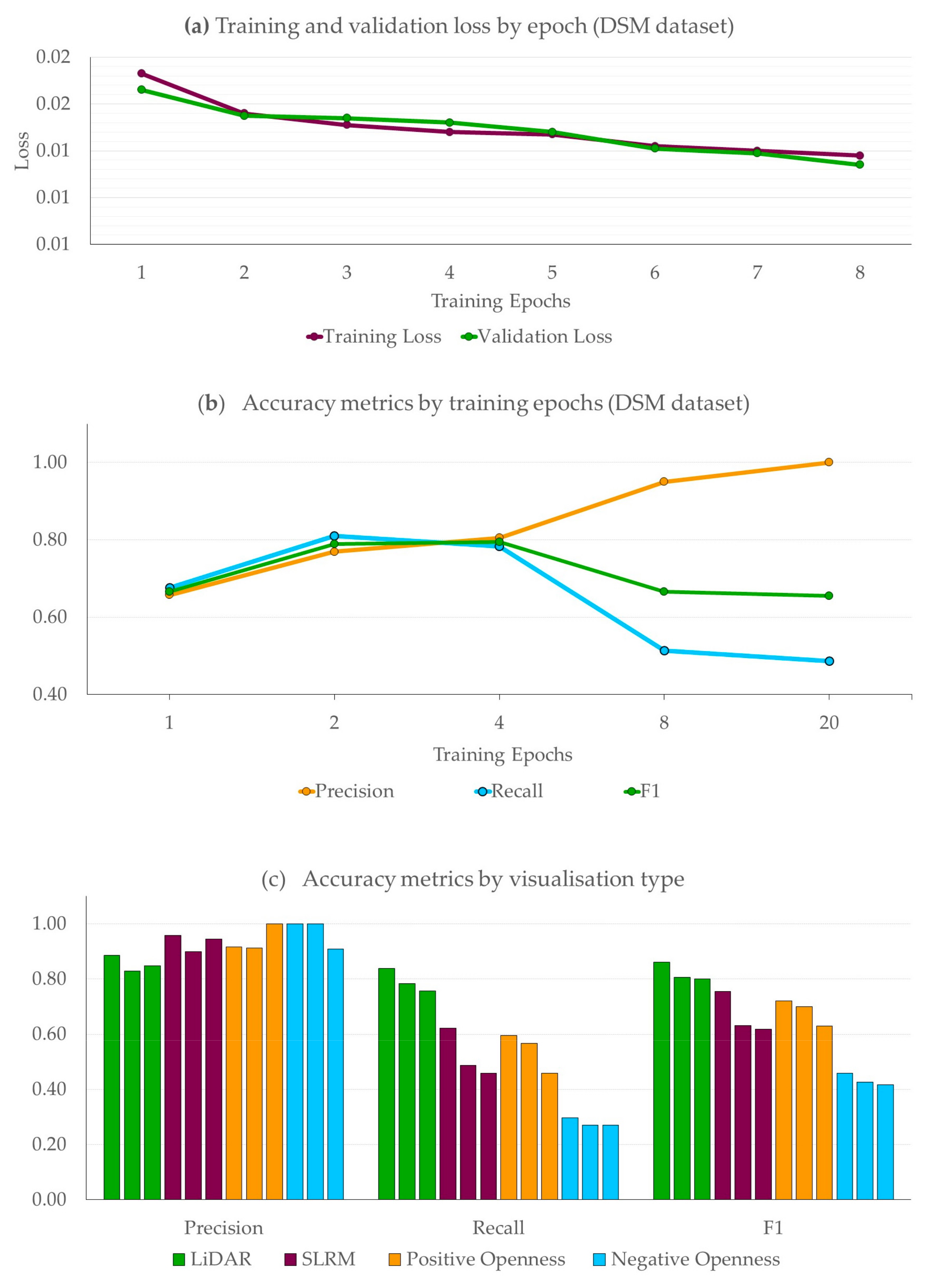
During training binary cross-entropy was used as the loss metric; the training loss began at approximately 0.02 for the DSM and between 0.03–0.04 for the other visualization types, reducing to an average of 0.0146 for all data types after four epochs. There was negligible variation in the loss by visualization type. The cross validation loss remained within 0.005 of the training loss for each epoch with the average cross validation loss 0.0145 after four epochs. However, during human examination of the output masks it was observed that because the model is attempting to lower the global loss over every pixel, the numeric values output from the TensorFlow console did not fully describe the real effectiveness of the model for detecting pit objects. This is suspected to be due to the fact that the model loss is a pixel based loss function rather than an object based one. Figure 8a displays the losses per epoch; showing that whilst the cross validation loss continues to decrease after four epochs, when compared to the F1 score shown in Figure 8b it can be seen that the real detection accuracy degrades after four epochs.
In light of this, a much smaller human cross validation was carried out on five sample tiles from the cross validation dataset. These tiles were visually chosen after inspecting all tiles in the validation dataset to asses each model’s performance at both ends of the difficulty spectrum, from simple cases with several well defined pits to complex cases with multiple ill-defined and overlapping pits or pits within larger trenches. To determine the optimal fine-tuning strategy, the number of epochs for which the model was retrained was varied and the results were examined by counting the detection instances over these tiles.
For each model and each tile, the number of true positives (correctly detected pits), false negatives (undetected pits) and false positives (detections which do not correspond to true pits) were counted. From these numbers the precision (the proportion of the model’s pit predictions that were correct) and the recall (the proportion of actual pits that were detected) were calculated. The F1 score (harmonic mean of precision and recall) was also calculated, as it is a useful single valued accuracy metric for a detection problem of this kind (formulas defined in Table 2). Due to the variability of deep learning model convergence, training will not produce identical results every time, to account for this each test was run three times and averaged. Figure 8b shows how the precision, recall and F1 scores vary as the number of fine-tuning epochs is increased. It should be noted that this figure shows accuracy metrics over only 5 tiles from the validation dataset, chosen for their difficulty to evaluate model generalization ability. Therefore, it does not represent the accuracy obtained by the model on the test datasets. It can be seen that the best results are found after three to four epochs of training. The degradation of accuracy after four epochs could correspond to overfitting; because each epoch trains the model using the same 520 test images, albeit augmented differently each time. As another test, the DeepMoon model was also run directly on the Dartmoor data without any fine-tuning training, this gave detection rates of approximately 40% with a bias towards large pits more similar in appearance to impact craters.
Once the optimal amount of fine tuning was determined, the four advanced visualization types were tested against the same five sample images. Each of the visualization types depicted previously in Figure 5 were used as the training data input for fine tuning the model. Using the knowledge from the previous validation test, the models were trained for four epochs, as before, each test was run three times and averaged. Longer training runs of eight epochs were also tested. This is to account for the possibility that due to the greater difference between some of the visualization styles and the model’s original lunar DSM training data more epochs might be required to obtain strong results. However, these tests displayed the same behavior as that shown in Figure 8b. It can be seen from Figure 8c that whilst the precision is high for all four data representations, the recall and therefore the F1 score is poorer for the advanced visualizations.
3.2. Test Area Results
The cross-validation results informed the development of the final model, which was then evaluated on the final unseen test datasets. The model was evaluated on a 1km2 tile of LiDAR data in Dartmoor approximately 20 km away from the training area. An additional test was carried out on a 0.2 km2 of Yorkshire more than 500 km away from the training data. The results obtained are summarized in Table 2. For both sets of results the highest performing model from the validation dataset was used for the predictions. It must be noted that these results have been calculated from the binary results mask. Of the missed detections 23 out of the 38 in Dartmoor and 17 out of 30 in Yorkshire are still visibly predicted in the full transparency results layer. This is because they fall below the 0.5 probability threshold used in the binary masking operation, thereby removing them from the count.
To further investigate the model’s generalization capabilities for additional archaeological object detection, a final experiment was carried out. For this, the model was run directly on 1m resolution LiDAR from the same section of Machie Moor (Arran, Scotland) as that tested by Trier et al. [32]. To validate, the true roundhouse locations were taken from [32]. In this experiment no additional training was carried out and the Dartmoor model was applied in its naive state. The results show the model generalized well considering the lack of training, with a precision rate of 0.55 and a recall rate of 0.45. This suggests real potential if trained for this type of feature detection. These results are consistent with how the original DeepMoon naive model performed on the Dartmoor data before fine tuning training was undertaken. From these results it is hoped that by introducing limited amounts of training data for other features of interest, this model is capable of being applied to a wide range of archaeological prospection problems.
4. Discussion
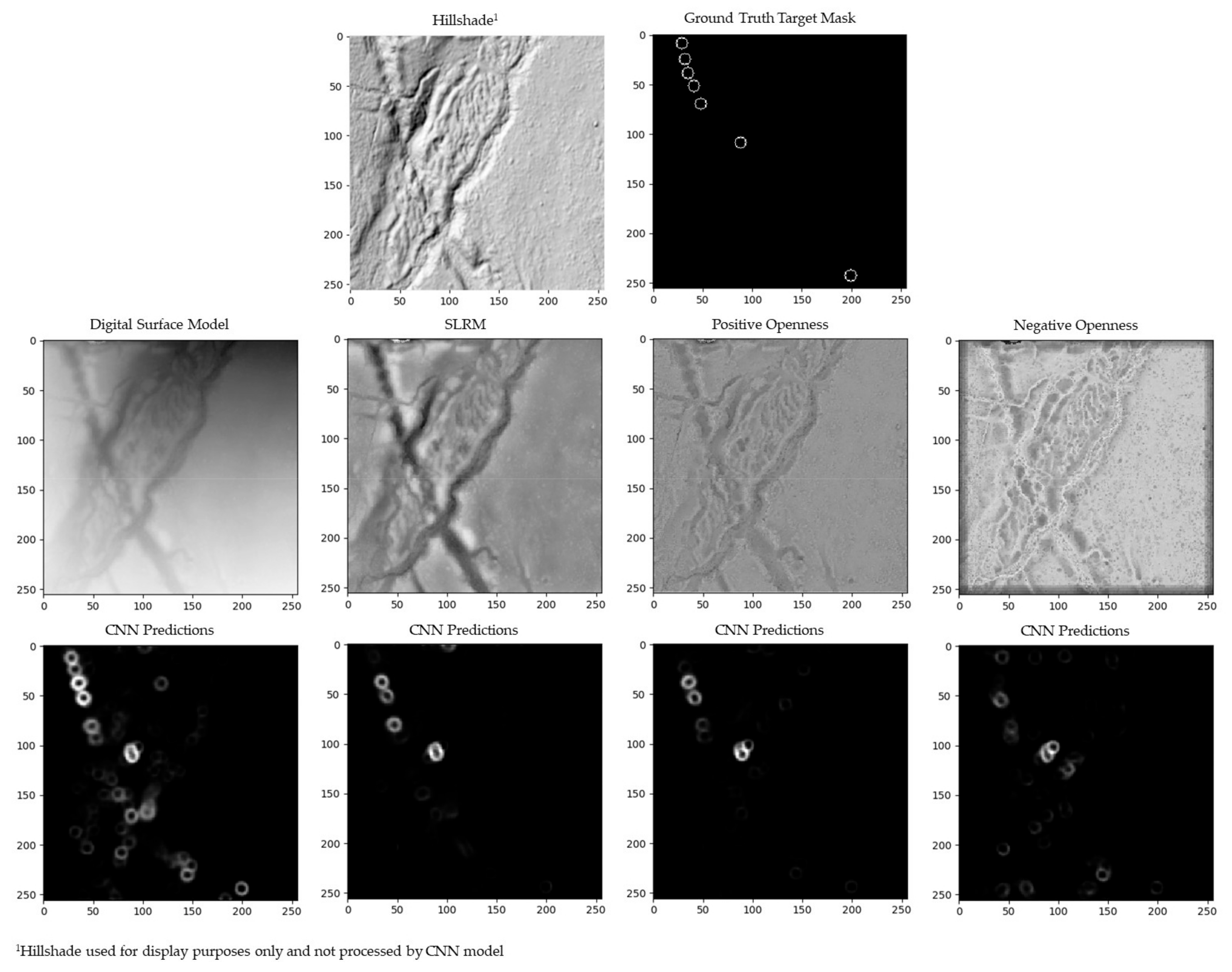
The cross-validation results from the different types of LiDAR visualizations indicated that the model performed better when trained on the raw 8-bit DSM height values rather than any of the advanced visualizations. It is suspected that whilst these visualizations are effective for human interpretation of archaeological data [11] and also effective for more traditional machine learning techniques [22], because deep CNNs learn their own feature representations during training, it is not desirable to artificially alter the data representation prior to input. However, it also must be taken into account that the CNN chosen in this study was pretrained on 8-bit DSM height values, thereby introducing a bias towards this representation. To fully test which LiDAR visualization is best suited for CNNs in future, would require a robust CNN trained from scratch on multiple differently visualized representations of the same data; however, such a model has not been made publicly available from any known sources at this time. To attempt to test this theory with the existing datasets experiments were carried out to create a model from scratch using the DeepMoon architecture and the Dartmoor training data with different visualizations. However, no meaningful results were obtained from any visualization, presumably due to the limited size of the training data. The SLRM and openness visualizations are included in this study as discussion points, to observe how the predictions vary and to provide stimulation for future work. An example of the predictions on a single challenging tile for each visualization type is shown in Figure 9. It can be seen that the predictions from the raw DSM are the most sensitive, resulting in the least amount of missed detections, and is the only one that picks up the isolated pit in the lower right corner. The confusion areas of low probability are easily filtered out by setting a probability threshold of 0.5 in the post-processing steps, as discussed in Section 2.6.
The final test area results demonstrate that the model is highly effective with the correct detections greatly outnumbering the missed and false detections, displaying strong precision and recall simultaneously. Precision and recall figures concurrently above 0.8 has not been achieved to date by any other deep learning tool for archaeological prospection [33], however, as there is no standard archaeological test dataset different approaches are not directly comparable, though the results obtained here clearly indicate this model has achieved state of the art results.
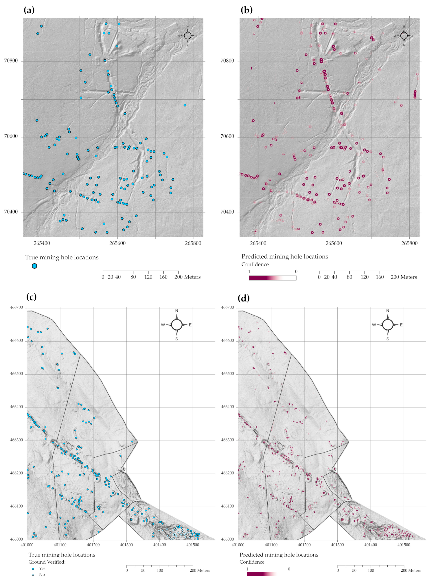
Figure 10 shows the full transparency results overlaid on the Dartmoor and Yorkshire test datasets. This figure shows that the model is highly capable of discerning mining pits and is not overwhelmed by false positives. It also demonstrates that even if individual detections might not always be correct the greater trends in the landscape are very clearly reproduced by the model. This is in line with the recommendations from Cowley for ‘a key conceptual shift from a widely held fixation in archaeology on individual identifications being correct to overall patterns being descriptive’ [3]. From a management perspective, these automatically generated maps clearly delineate the extents and key structures of these historic mining sites, with limited confusion areas due to model assumptions and landscape morphology.
In Figure 10a,b small confusion areas can be seen around the ends of larger openworked trenches. This is due to the fact that the model is making predictions on cropped image tiles; if only the end of the trench is visible in the tile, the model’s strong generalization ability works against it and it will predict a semi-circular occluded hole. As the tiles have 52% overlap these false positives are typically removed by the raster mosaic post processing step, however, due to anomalies in position and tile overlap, some remain.
The Yorkshire test as shown in Figure 10c,d was carried out to examine the model’s ability to generalize to different types of mines and different resolution data. The model surpassed its previous performance on this dataset, as shown in Table 2. The Yorkshire LiDAR DSM is twice the resolution of the Dartmoor data at 0.25 m but contains more confusion objects such as building remains, stone lined trenches and drainage culverts. The model was capable of discriminating between building foundation remains and excavated platforms from mining pits and made only two false positive detections in these areas. This is an extremely positive result and indicated the model is doing more than just looking for unnatural changes in ground elevation and is searching instead for areas that contain the features which it was trained on.
Of the mistakes, one drainage culvert was mistaken for a hole, but the geometry was such that is was only discernible as a culvert from a side view under the road unafforded to the LiDAR data. This is a limitation of all overhead remotely sensed data and is not specific to a deep learning model. Two trenches were misidentified as pits but only where dense vegetation masked their linearity causing them to appear as circular depressions on the LiDAR.
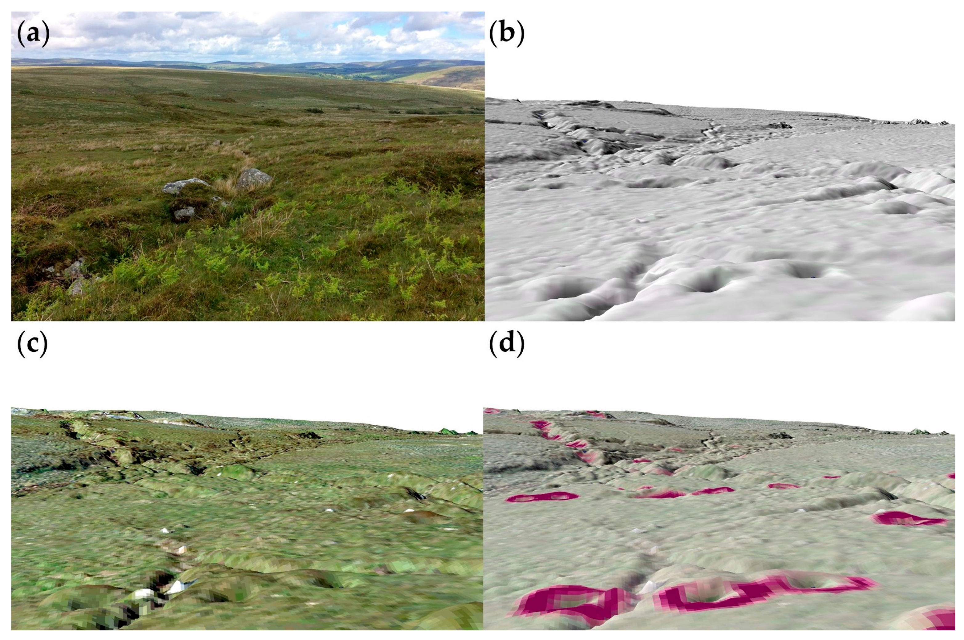
The site verification visits revealed that many of the detected pits would be difficult to locate either on foot or from aerial photography as they are faint, shallow and reed-filled. Whilst ground truthing many pits were near-invisible until the surveyor was within a few meters of the model’s predicted location; as well, whilst traversing the sites to verify the predictions, no isolated pits were seen that were missed by the model, all missed detections were within larger excavations that had caused confusion. Figure 11 shows a photograph taken looking north from the Hexworthy site, aligned with the same view from the LiDAR model overlaid with aerial imagery and predicted hole locations.
The results from the two tests indicate that this model is able to generalize to new sites and that higher resolution LiDAR improves classification accuracy. These tests also show that despite being trained on one resolution of data the model is capable of being applied at a different resolution without the need for additional training, greatly increasing its applicability for varying quality and resolution general purpose LiDAR datasets. This is crucial as most LiDAR is not flown specifically for archeological site detection purposes; therefore, site detection algorithms must be capable of working with varying accuracy and resolution datasets gathered by many agencies for diverse reasons.
This model is a single class segmenter; therefore, to extend the model to more general archaeological prospection tasks multiple models must be trained for different classes. Whist this could be considered a weakness of this approach, no other work to date has managed to fully optimize models for multiple classes simultaneously, despite architectures which permit multiclass outputs. Verschoof-van der Vaart and Lambers [33] successfully trained a multi-class detector and achieved high F1 scores in both classes, however, the highest F1 scores per class did not occur simultaneously. Multi-class learning is more difficult than single class learning, and the problem of automated archaeological site detection is also more difficult than general image classification, due to the small amount of training data and the subtlety of the detections required. It is proposed that at this early stage, development of accurate single class detectors which can be stacked into multi-layer images will produce the most effective, repeatable and easily usable results. These detectors do not have to be trained for every type of potential feature, an approach which would be neither achievable nor desirable, but rather trained to detect general areas of suspicious topology in several broad categories, flagging it for further inspection, leaving the interpretation to humans for now. The results shown in this study prove that as a first part of a multi-stage phased landscape analysis this model is capable and effective. Delineation and quantification of sites using an approach such as this would add to the body of knowledge about such sites, provide impetus for further surveys and underpin protection of these sites from future threats.
The mining pit detection model created here can be rapidly run on any LiDAR DSM suspected of containing remains of historic mining activity; the approximate time to process a 1km tile including manual ArcGIS post-processing is 5 min. This pipeline could be easily automated further, as this research has been concerned with the ultimate performance of the deep learning model the periphery workflow has not yet been streamlined. As an output, simple GIS point layers (with their accuracy specifications of ± 20%) can be supplied to the land managers such as Dartmoor National Park and Yorkshire Dales National Park. These results are usable directly by the land managers to rapidly inform future decisions about preservation and management.
A model trained for a different type of site detection could be applied similarly, provided the appropriate training and testing had been carried out. Development of these new models is an exciting direction for further research. The logical next step would be to trial this model on a well-researched study area such as Arran [4], with the aim of developing accurate general purpose, large scale semi-automated site detection tools in the near future.
5. Conclusions
The transfer learning model developed in this research shows strong, repeatable results for the task of detecting historic mining pits, alongside promising generalization abilities for other similar tasks. It is a novel application of knowledge from the disparate but related field of planetary remote sensing, achieving state of the art results on its allocated task. It is capable of differentiating between natural depressions and manmade ones, even in areas of occlusion and erosion. This is due to the close resemblance between the data on which the base model was pretrained and the data for the problem at hand. Other strengths of this model are its ability to output full pixelwise segmented confidence masks for any size and resolution data, alongside this workflow’s integration with existing ArcGIS tools where possible to ensure ease of use and repeatability.
This research builds on the work of Trier et al. [32] and Verschoof-van der Vaart and Lambers [33] by following their recommendations to seek closely applicable transfer learning models for deep learning on archaeological LiDAR data. It is hoped that this model will prove suitable for other archaeological prospection tasks when furnished with applicable training data. The initial naive applicability test using the Arran data showed promising results for future work in this direction.
This model can run on large swathes of LiDAR data extremely quickly and produces meaningful results which will aid interpretation of large scale historic mining landscapes. The model is also valuable for detecting outlying smaller pits away from the main shafts and mineral veins. These are often unrecorded remains of earlier prospecting and information on their location can add to understanding of a site’s exploitation history. It is envisaged that this model would be run as a first step in the prospection process, vastly reducing the areas to be analyzed in fine detail in a desktop search or fieldwork survey by a mining historian. With a false positive rate of less than 20% it does not overwhelm the analyst with incorrect predictions, providing an effective tool for preliminary site investigation and allowing confidence in the use of the model. The workflow and model presented here will allow the scale and magnitude of sites to be rapidly analyzed, underpinning better cultural heritage management decisions for these valuable records of our industrial past.
Supplementary Materials
The following are available online at https://www.mdpi.com/2072-4292/11/17/1994/s1, Workflow document: S1, Model S2: Deep learning model.
Author Contributions
Conceptualization, M.E. and J.G.; investigation, J.G.; methodology, J.G.; software, J.G. and M.T.; validation, J.G.; writing—original draft preparation, J.G.; writing—review and editing, M.E. and J.C.; supervision, M.E. and J.C.
Funding
This research received no external funding.
Conflicts of Interest
The authors declare no conflict of interest.
References
- Bewley, R.H.; Crutchley, S.P.; Shell, C.A. New light on an ancient landscape: Lidar survey in the Stonehenge World Heritage Site. Antiquity 2005, 79, 636–647. [Google Scholar] [CrossRef]
- Moyes, H.; Montgomery, S. Locating Cave Entrances Using Lidar-Derived Local Relief Modeling. Geosciences 2019, 9, 98. [Google Scholar] [CrossRef]
- Cowley, D.C. In with the new, out with the old? Auto-extraction for remote sensing archaeology. Remote Sens. Ocean Sea Ice Coast Waters Large Water Reg. 2012, 8532, 853206. [Google Scholar] [CrossRef]
- Banaszek, Ł.; Cowley, D.; Middleton, M. Towards National Archaeological Mapping. Assessing Source Data and Methodology—A Case Study from Scotland. Geosciences 2018, 8, 272. [Google Scholar] [CrossRef]
- Bennett, R.; Cowley, D.; De Laet, V. The data explosion: Tackling the taboo of automatic feature recognition in airborne survey data. Antiquity 2014, 88, 896–905. [Google Scholar] [CrossRef]
- Winter, S. Uncovering England’s Landscape by 2020. Available online: https://environmentagency.blog.gov.uk/2017/12/30/uncovering-englands-landscape-by-2020/ (accessed on 9 June 2019).
- Hesse, R. The changing picture of archaeological landscapes: Lidar prospection over very large areas as part of a cultural heritage strategy. In Interpreting Archaeological Topography: 3D Data, Visualisation and Observation; Opitz, R.S., Cowley, D.C., Eds.; Oxbow: Oxford, UK, 2013; pp. 171–183. [Google Scholar]
- Brightman, J.; White, R.; Johnson, M. Landscape-Scale Assessment: A Pilot Study Using the Yorkshire Dales Historic Environment. 2015; Unpublished Historic England report number 7049, available upon request from Historic England. [Google Scholar]
- Loren-Méndez, M.; Pinzón-Ayala, D.; Ruiz, R.; Alonso-Jiménez, R. Mapping Heritage: Geospatial Online Databases of Historic Roads. The Case of the N-340 Roadway Corridor on the Spanish Mediterranean. ISPRS Int. J. Geo-Inf. 2018, 7, 134. [Google Scholar] [CrossRef]
- Kokalj, Ž.; Hesse, R. Airborne Laser Scanning Raster Data Visualization. A Guide to Good Practice; Prostor, K.C., Ed.; Založba ZRC: Ljubljana, Slovenia, 2017; Volume 14, ISBN 12549848. [Google Scholar]
- Kokalj, Ž.; Somrak, M. Why Not a Single Image? Combining Visualizations to Facilitate Fieldwork and On-Screen Mapping. Remote Sens. 2019, 11, 747. [Google Scholar] [CrossRef]
- Jacobson, N.P.; Gupta, M.R. Design Goals and Solutions for Display of Hyperspectral Images. IEEE Trans. Geosci. Remote Sens. 2005, 43, 2684–2692. [Google Scholar] [CrossRef]
- Cowley, D.C. What do the patterns mean? Archaeological distributions and bias in survey data. In Digital Methods and Remote Sensing in Archaeology; Springer: Cham, Switzerland, 2016; pp. 147–170. [Google Scholar]
- Lambers, K.; Verschoof-van der Vaart, W.B.; Bourgeois, Q.P.J. Integrating remote sensing, machine learning, and citizen science in dutch archaeological prospection. Remote Sens. 2019, 11, 1–20. [Google Scholar] [CrossRef]
- Duckers, G.L. Bridging the ‘geospatial divide’in archaeology: Community based interpretation of LIDAR data. Internet Archaeol. 2013, 35. [Google Scholar] [CrossRef]
- Morrison, W.; Peveler, E. Beacons of the Past Visualising LiDAR on a Large Scale; Chilterns Conservation Board: Chinnor, UK, 2016. [Google Scholar]
- Trier, Ø.D.; Larsen, S.Ø.; Solberg, R. Automatic Detection of Circular Structures in High-resolution Satellite Images of Agricultural Land. Archaeol. Prospect. 2009, 16, 1–15. [Google Scholar] [CrossRef]
- Trier, Ø.D.; Zortea, M.; Tonning, C. Automatic detection of mound structures in airborne laser scanning data. J. Archaeol. Sci. Rep. 2015, 2, 69–79. [Google Scholar] [CrossRef]
- Sevara, C.; Pregesbauer, M.; Doneus, M.; Verhoeven, G.; Trinks, I. Pixel versus object—A comparison of strategies for the semi-automated mapping of archaeological features using airborne laser scanning data. J. Archaeol. Sci. Rep. 2016, 5, 485–498. [Google Scholar] [CrossRef]
- Freeland, T.; Heung, B.; Burley, D.V.; Clark, G.; Knudby, A. Automated feature extraction for prospection and analysis of monumental earthworks from aerial LiDAR in the Kingdom of Tonga. J. Archaeol. Sci. 2016, 69, 64–74. [Google Scholar] [CrossRef]
- Trier, Ø.D.; Salberg, A.-B.; Pilø, L.H. Semi-automatic mapping of charcoal kilns from airborne laser scanning data using deep learning. In Proceedings of the 44th Conference on Computer Applications and Quantitative Methods in Archaeology, Oslo, Norway, 29 March–2 April 2016; Matsumoto, M., Uleberg, E., Eds.; Archaeopress: Oxford, UK, 2018; pp. 219–231. [Google Scholar]
- Guyot, A.; Hubert-Moy, L.; Lorho, T. Detecting Neolithic burial mounds from LiDAR-derived elevation data using a multi-scale approach and machine learning techniques. Remote Sens. 2018, 10, 225. [Google Scholar] [CrossRef]
- Gao, H.; Mao, J.; Zhou, J.; Huang, Z.; Wang, L.; Xu, W. Are you talking to a machine? Dataset and methods for multilingual image question answering. In Proceedings of the Advances in Neural Information Processing Systems, Motreal, QC, Canada, 7–12 December 2015; pp. 1–10. [Google Scholar]
- Redmon, J.; Farhadi, A. YOLO9000 Better, stronger, faster. In Proceedings of the IEEE Conference on Computer Vision and Pattern Recognition, Las Vegas, NV, USA, 26 June–1 July 2016; pp. 7263–7271. [Google Scholar]
- Sun, Y.; Zhang, X.; Xin, Q.; Huang, J. Developing a multi-filter convolutional neural network for semantic segmentation using high-resolution aerial imagery and LiDAR data. ISPRS J. Photogramm. Remote Sens. 2018, 143, 3–14. [Google Scholar] [CrossRef]
- Cheng, G.; Zhou, P.; Han, J. Learning Rotation-Invariant Convolutional Neural Networks for Object Detection in VHR Optical Remote Sensing Images. IEEE Trans. Geosci. Remote Sens. 2016, 54, 7405–7415. [Google Scholar] [CrossRef]
- Ren, Y.; Zhu, C.; Xiao, S. Small Object Detection in Optical Remote Sensing Images via Modified Faster R-CNN. Appl. Sci. 2018, 8, 813. [Google Scholar] [CrossRef]
- Nogueira, K.; Penatti, O.A.B.; dos Santos, J.A. Towards better exploiting convolutional neural networks for remote sensing scene classification. Pattern Recognit. 2017, 61, 539–556. [Google Scholar] [CrossRef] [Green Version]
- Razavian, A.S.; Azizpour, H.; Sullivan, J.; Carlsson, S. CNN features off-the-shelf: An astounding baseline for recognition. In Proceedings of the IEEE CVPR Workshop, Columbus, OH, USA, 23–28 June 2014; pp. 512–519. [Google Scholar] [CrossRef]
- Deng, J.; Dong, W.; Socher, R.; Li, L.-J.; Li, K.; Fei-Fei, L. ImageNet: A Large-Scale Hierarchical Image Database. In Proceedings of the CVPR09, Miami, FL, USA, 22–24 June 2009. [Google Scholar]
- Ball, J.E.; Anderson, D.T.; Chan, C.S. Comprehensive Survey of Deep Learning in Remote Sensing: Theories, Tools and Challenges for the Community. J. Appl. Remote Sens. 2017, 11. [Google Scholar] [CrossRef]
- Trier, Ø.D.; Cowley, D.C.; Waldeland, A.U. Using deep neural networks on airborne laser scanning data: Results from a case study of semi-automatic mapping of archaeological topography on Arran, Scotland. Archaeol. Prospect. 2019, 26, 165–175. [Google Scholar] [CrossRef]
- Verschoof-van der Vaart, W.B.; Lambers, K. Learning to Look at LiDAR: The use of R-CNN in the automated detection of archaeological objects in LiDAR data from the Netherlands. J. Comput. Appl. Archaeol. 2019, 2, 31–40. [Google Scholar] [CrossRef]
- Hesse, R. LiDAR-derived Local Relief Models—A new tool for archaeological prospection. Archaeol. Prospect. 2010, 17, 67–72. [Google Scholar] [CrossRef]
- Zuber, M.T.; Smith, D.E.; Zellar, R.S.; Neumann, G.A.; Sun, X.; Katz, R.B.; Kleyner, I.; Matuszeski, A.; McGarry, J.F.; Ott, M.N.; et al. The Lunar Reconnaissance Orbiter Laser Ranging Investigation. Space Sci. Rev. 2009, 150, 63–80. [Google Scholar] [CrossRef]
- Albee, A.L.; Arvidson, R.E.; Palluconi, F.; Thorpe, T. Overview of the Mars Global Surveyor mission. J. Geophys. Res. E Planets 2001, 106, 23291–23316. [Google Scholar] [CrossRef] [Green Version]
- Silburt, A.; Ali-Dib, M.; Zhu, C.; Jackson, A.; Valencia, D.; Kissin, Y.; Tamayo, D.; Menou, K. Lunar crater identification via deep learning. Icarus 2019, 317, 27–38. [Google Scholar] [CrossRef]
- Wang, H.; Jiang, J.; Zhang, G. CraterIDNet: An end-to-end fully convolutional neural network for crater detection and identification in remotely sensed planetary images. Remote Sens. 2018, 10, 67. [Google Scholar] [CrossRef]
- Palafox, L.F.; Hamilton, C.W.; Scheidt, S.P.; Alvarez, A.M. Automated detection of geological landforms on Mars using Convolutional Neural Networks. Comput. Geosci. 2017, 101, 48–56. [Google Scholar] [CrossRef]
- Ronneberger, O.; Fischer, P.; Brox, T. U-net: Convolutional networks for biomedical image segmentation. In Lecture Notes in Computer Science; Springer: Berlin, Germany, 2015; Volume 9351, pp. 234–241. [Google Scholar]
- Žutautas, V. Charcoal Kiln Detection from LiDAR-derived Digital Elevation Models Combining Morphometric Classification and Image Processing Techniques. Master’s Thesis, University of Gävle, Gävle, Sweden, 2017. [Google Scholar]
- Trier, Ø.; Zortea, M. Semi-automatic detection of cultural heritage in lidar data. In Proceedings of the 4th International Conference GEOBIA, Rio de Janeiro, Brazil, 7–9 May 2012; pp. 123–128. [Google Scholar]
- Davis, D.S.; Sanger, M.C.; Lipo, C.P. Automated mound detection using lidar and object-based image analysis in Beaufort County, South Carolina. J. Archaeol. Sci. 2018. [Google Scholar] [CrossRef]
- Newman, P. Environment, Antecedent and Adventure: Tin and Copper Mining on Dartmoor, Devon. Ph.D. Thesis, University of Leicester, Leicester, UK, 2010. [Google Scholar]
- Dines, H.G. The Metalliferous Mining Region of South West England, 3rd ed.; British Geological Survey: Nottingham, UK, 1988. [Google Scholar]
- Hamilton Jenkin, A.K. Mines of Devon Volume 1: The Southern Area; David and Charles (Holdings) Limited: Newton Abbot, UK, 1974. [Google Scholar]
- Richardson, P.H.G. British Mining Vol. 44: Mines of Dartmoor and the Tamar Valley; Northern Mine Research Society: Sheffield, UK, 1992. [Google Scholar]
- Northern Mine Research Society. British Mining No 13: The Mines of Grassington Moor; Northern Mine Research Society: Sheffield, UK, 1980. [Google Scholar]
- Lidar Composite Digital Surface Model England 50cm and 25 cm[ASC Geospatial Data], Scale 1:2000 and 1:1000, Tiles: sx6780, sx6781, sx6782, sx6880, sx6680, sx6681, sx6070, sx6071, sx6170, sx6171, sx6270, sx6570 and se0166. Available online: https://digimap.edina.ac.uk (accessed on 7 March 2019).
- Yeomans, C.M. Tellus South West data usage: A review (2014–2016). In Proceedings of the Open University Geological Society, Exeter, UK, April 2017; Hobbs the Printers Ltd.: Hampshire, UK, 2017; Volume 3, pp. 51–61. [Google Scholar]
- ESRI ArcGIS Pro 2.3.1. Available online: https://www.esri.com/en-us/arcgis/products/arcgis-pro/overview (accessed on 1 January 2019).
- 1:2500 County Series 1st Edition. [TIFF Geospatial Data], Scale 1:2500, Tiles: Devo-sx6780-1, devo-sx6781-1, devo-sx6782-1, devo-sx680-1, devo-sx6681-1, devo-sx6070-1, devo-sx6071-1, devo-sx6170-1, devo-sx6171-1, devo-sx6270-1 and devo-sx6570-1. Available online: https://digimap.edina.ac.uk (accessed on 7 March 2019).
- High Resolution (25cm) Vertical Aerial Imagery. (2011, 2015) Scale 1:500, Tiles: sx6780, sx6781, sx6782, sx6680, sx6681, sx6070, sx6071, sx6170, sx6171, sx6270, sx6570 and se0166, Updated: 25 October 2015, Getmapping, Using: EDINA Aerial Digimap Service. Available online: https://digimap.edina.ac.uk (accessed on 09 March 2019).
- Relief Visualisation Toolbox (RVT). Available online: https://iaps.zrc-sazu.si/en/rvt#v (accessed on 26 March 2019).
- Doneus, M. Openness as visualization technique for interpretative mapping of airborne lidar derived digital terrain models. Remote Sens. 2013, 5, 6427–6442. [Google Scholar] [CrossRef]
- Lecun, Y.; Bottou, L.; Bengio, Y.; Haffner, P. Gradient-based learning applied to document recognition. Proc. IEEE 1998, 86, 2278–2324. [Google Scholar] [CrossRef] [Green Version]
- Krizhevsky, A.; Sutskever, I.; Hinton, G.E. ImageNet Classification with Deep Convolutional Neural Networks Alex. Adv. Neural Inf. Process. Syst. 2012, 25, 1106–1114. [Google Scholar] [CrossRef]
- Goodfellow, I.; Bengio, Y.; Courville, A. Deep Learning; MIT Press: Cambridge, MA, USA, 2016. [Google Scholar]
- Girshick, R.; Donahue, J.; Darrell, T.; Malik, J. Rich feature hierarchies for accurate object detection and semantic segmentation. In Proceedings of the IEEE Conference on Computer Vision and Pattern Recognition, Columbus, OH, USA, 23–28 June 2014; pp. 580–587. [Google Scholar] [CrossRef]
- He, K.; Gkioxari, G.; Dollar, P.; Girshick, R. Mask R-CNN. In Proceedings of the IEEE International Conference on Computer Vision, Venice, Italy, 22–29 October 2017; IEEE: Piscataway, NJ, USA, 2017; pp. 2980–2988. [Google Scholar] [CrossRef]
- Szegedy, C.; Vanhoucke, V.; Ioffe, S.; Shlens, J.; Wojna, Z. Rethinking the Inception Architecture for Computer Vision. In Proceedings of the IEEE Conference on Computer Vision and Pattern Recognition, Las Vegas, NV, USA, 27–30 June 2016; pp. 2818–2826. [Google Scholar] [CrossRef]
- Lin, T.Y.; Maire, M.; Belongie, S.; Hays, J.; Perona, P.; Ramanan, D.; Dollár, P.; Zitnick, C.L. Microsoft COCO: Common objects in context. In Lecture Notes in Computer Science; Springer: Berlin, Germany, 2014; Volume 8693, pp. 740–755. [Google Scholar]
- Badrinarayanan, V.; Kendall, A.; Cipolla, R. Segnet: A deep convolutional encoder-decoder architecture for image segmentation. IEEE Trans. Pattern Anal. Mach. Intell. 2017, 39, 2481–2495. [Google Scholar] [CrossRef] [PubMed]
- Python 3.6.7. Available online: https://www.python.org (accessed on 14 August 2019).
- Abadi, M.; Agarwal, A.; Barham, P.; Brevdo, E.; Chen, Z.; Citro, C.; Corrado, G.S.; Davis, A.; Dean, J.; Devin, M.; et al. TensorFlow: Large-scale machine learning on heterogeneous systems. arXiv 2015, arXiv:1603.04467. [Google Scholar]
- Chollet, F. Keras 2015. Available online: https://keras.io (accessed on 14 August 2019).
Figure 1.
Overview of the Dartmoor dataset. Grey areas represent training data (14 tiles), the purple tile shows the cross validation area and the orange tile shows the test area. Coordinate system British National Grid, image data © Environment Agency 2015 & Getmapping Plc. Basemap © ESRI 2019.
Figure 1.
Overview of the Dartmoor dataset. Grey areas represent training data (14 tiles), the purple tile shows the cross validation area and the orange tile shows the test area. Coordinate system British National Grid, image data © Environment Agency 2015 & Getmapping Plc. Basemap © ESRI 2019.

Figure 2.
Examples of the historic mining objects found in this study displayed on a 315° azimuth 35° sun elevation hillshaded visualization created in ArcGIS. Base DSM © Environment Agency 2015.
Figure 2.
Examples of the historic mining objects found in this study displayed on a 315° azimuth 35° sun elevation hillshaded visualization created in ArcGIS. Base DSM © Environment Agency 2015.

Figure 3.
Methodology process diagram. Full details of the processing steps are provided in Supplementary Document S1.
Figure 3.
Methodology process diagram. Full details of the processing steps are provided in Supplementary Document S1.

Figure 4.
Overview of image preprocessing pipeline. (a) shows a selection of original individual pixel values, (b) shows the same pixels rescales between 0 and 1. (c) shows the conversion to greyscale. For subimages (a–c) the actual greyscale value does not change as the range is still determined by the elevation range across the original 1 km × 1 km DSM tile, in this simple example this is set as 20 m. (d) shows the pixel values after linearly rescaling by tile range.

Figure 5.
Illustration of the different advanced visualizations created from the original LiDAR DSM. Base DSM © Environment Agency 2015, visualizations created using the Relief Visualization Toolbox [54].
Figure 5.
Illustration of the different advanced visualizations created from the original LiDAR DSM. Base DSM © Environment Agency 2015, visualizations created using the Relief Visualization Toolbox [54].

Figure 6.
Examples of the input data to different pretrained models. (a) is an example from the Common Objects in Context (COCO) [62] dataset which many existing models are trained with and is similar to the image type found in ImageNet [30] and other natural photography datasets. (b) and (c) show the results from an object detector pre-trained using the COCO dataset. It can be seen that whilst it makes many correct detections there are also many missed pits. (d) shows the type of microscopy data which the U-net architecture was designed to segment [40] and (e) shows data from the lunar DSM which was used to pre-train the model used in this research [37]. (f) shows the DSM data used in this project. Base DSM in (b,c,f) © Environment Agency 2015.

Figure 7.
Comparison of qualitative and quantitative results representations. (a) shows the ground truth locations of a section of very shallow (30–50 cm depth) mining pits in the Hexworthy test area. (b) shows the model’s predicted results depicted with a graduated transparency color scale representing model confidence and (c) shows a binary mask where all prediction pixels above 0.4 are assigned as ‘pit’ and all others are discarded. DSM © Environment Agency 2015.

Figure 8.
Training and validation loss by epoch across the entire validation dataset (a). Accuracy metrics by training epochs (b) and accuracy metrics by visualization type (c), both evaluated on sample tiles from the validation dataset. Note: (b) and (c) show accuracy metrics over only 5 tiles from the validation dataset chosen for their difficulty to evaluate model generalization ability. Therefore, they do not represent the accuracy obtained by the model on the test datasets.

Figure 9.
Results from a single image tile for each of the different visualization predictions. 1Hillshade used for display purposes only and not processed by the CNN model. Coordinate system arbitrary pixel based.
Figure 9.
Results from a single image tile for each of the different visualization predictions. 1Hillshade used for display purposes only and not processed by the CNN model. Coordinate system arbitrary pixel based.

Figure 10.
Results overlaid on hillshaded LiDAR. (a,b) are from the Dartmoor Hexworthy mine test area, Ordnance Survey grid tile SX6570. (a) shows the true mining hole locations in blue and (b) shows the model’s predicted mining hole locations in magenta. (c) and (d) show the results from the Yorkshire Yarnbury mine test area, Ordnance Survey grid tile SE0166. (c) shows the true mining hole locations in blue and (d) shows the model’s predicted mining hole locations in magenta. In the extensively mined area to the southeast it was not possible to ground verify precise locations as it was fenced off as a hazardous area, however, a visual inspection confirmed many pits and shafts present thereabouts. Their locations were determined from a desktop search and are marked accordingly in (c). Coordinate system British National Grid, DSM © Environment Agency 2015.

Figure 11.
Ground level view of the Hexworthy historic mine site. (a) is a photograph taken during the verification survey, (b) shows the same scene in a hillshaded DSM, (c) includes OSGB 2010 aerial imagery and (d) includes the model’s predictions. DSM and aerial imagery © Environment Agency 2015 & Digimap Getmapping Plc.


Table 1.
Dataset statistics.
| Dataset | Image Tiles | Pit Ground | Pit Instances | Minimum | Mean | Maximum |
|---|---|---|---|---|---|---|
| Train | 542 | 1568 | 3649 | 1 | 5.96 | 59 |
| Cross-validate | 71 | 254 | 423 | 1 | 5.96 | 33 |
| Test Dartmoor | 196 | 193 | 654 | 1 | 5.74 | 24 |
| Test Yorkshire | 900 | 172 1 | n/a 2 | n/a 2 | n/a 2 | n/a 2 |
1 Only pits within a section of the dataset were ground truthed as shown in Figure 10c. 2 The Yorkshire dataset was exported for testing without human generated labels.
Table 2.
Full results from test datasets.
| Test Area | True Positives | False Positives | False Negatives | Precision 1 | Recall 2 | F1 3 |
|---|---|---|---|---|---|---|
| Dartmoor | 155 | 37 | 38 | 0.81 | 0.80 | 0.81 |
| Yorkshire | 142 | 13 | 30 | 0.92 | 0.83 | 0.87 |
1 Precision = True Positives/(True Positives + False Positives), 2 Recall = True Positives/(True Positives + False Negatives), 3 F1 = 2 × ((Precision × Recall)/(Precision + Recall)).
© 2019 by the authors. Licensee MDPI, Basel, Switzerland. This article is an open access article distributed under the terms and conditions of the Creative Commons Attribution (CC BY) license (http://creativecommons.org/licenses/by/4.0/).
Share and Cite
MDPI and ACS Style
Gallwey, J.; Eyre, M.; Tonkins, M.; Coggan, J. Bringing Lunar LiDAR Back Down to Earth: Mapping Our Industrial Heritage through Deep Transfer Learning. Remote Sens. 2019, 11, 1994. https://doi.org/10.3390/rs11171994
AMA Style
Gallwey J, Eyre M, Tonkins M, Coggan J. Bringing Lunar LiDAR Back Down to Earth: Mapping Our Industrial Heritage through Deep Transfer Learning. Remote Sensing. 2019; 11(17):1994. https://doi.org/10.3390/rs11171994
Chicago/Turabian StyleGallwey, Jane, Matthew Eyre, Matthew Tonkins, and John Coggan. 2019. "Bringing Lunar LiDAR Back Down to Earth: Mapping Our Industrial Heritage through Deep Transfer Learning" Remote Sensing 11, no. 17: 1994. https://doi.org/10.3390/rs11171994
Note that from the first issue of 2016, this journal uses article numbers instead of page numbers. See further details here.