Comparison of Passive Microwave Data with Shipborne Photographic Observations of Summer Sea Ice Concentration along an Arctic Cruise Path


Abstract
:
1. Introduction
2. Data and Methods
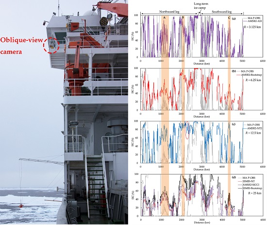
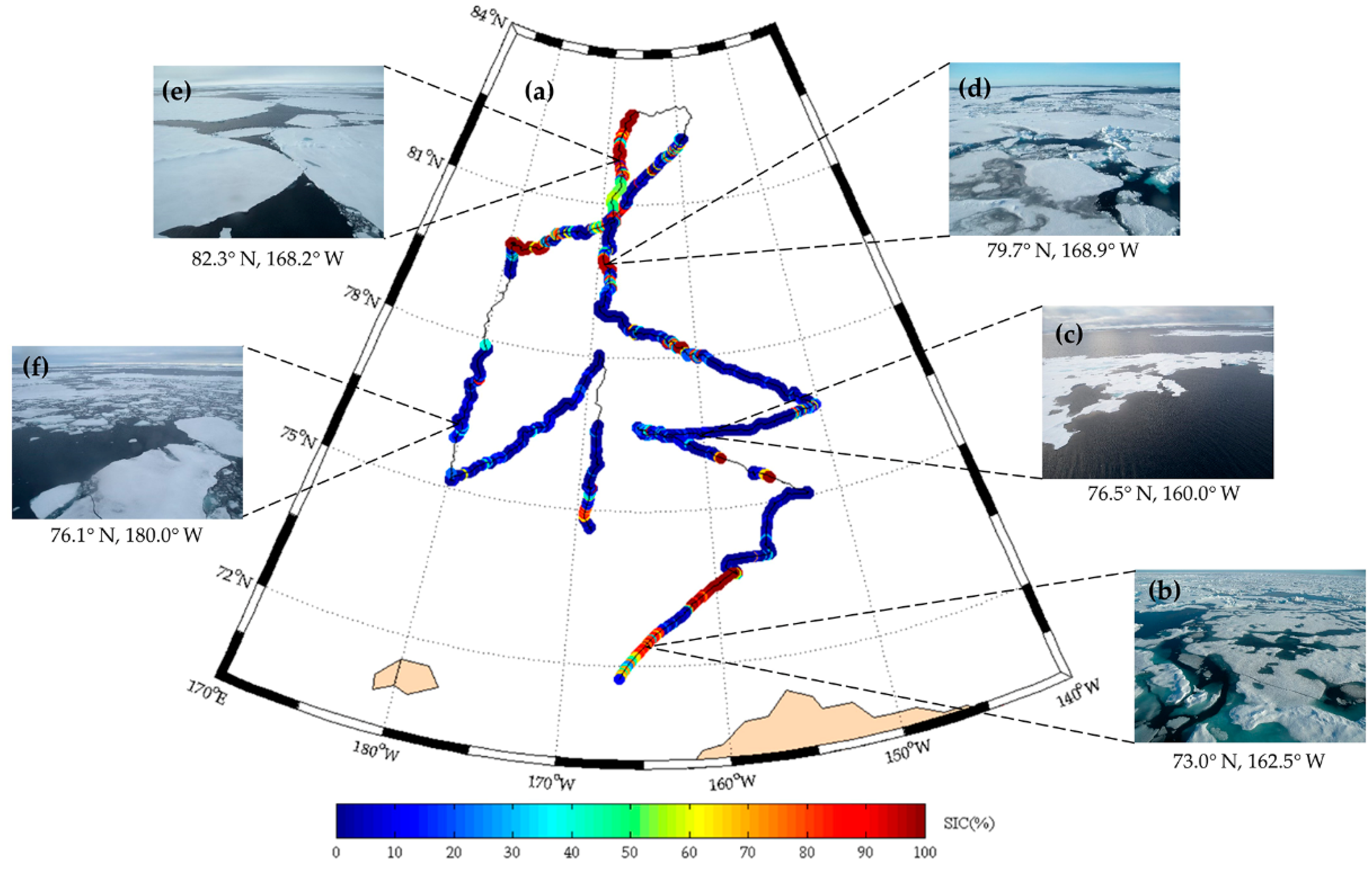
2.1. Overview of Ice Navigation
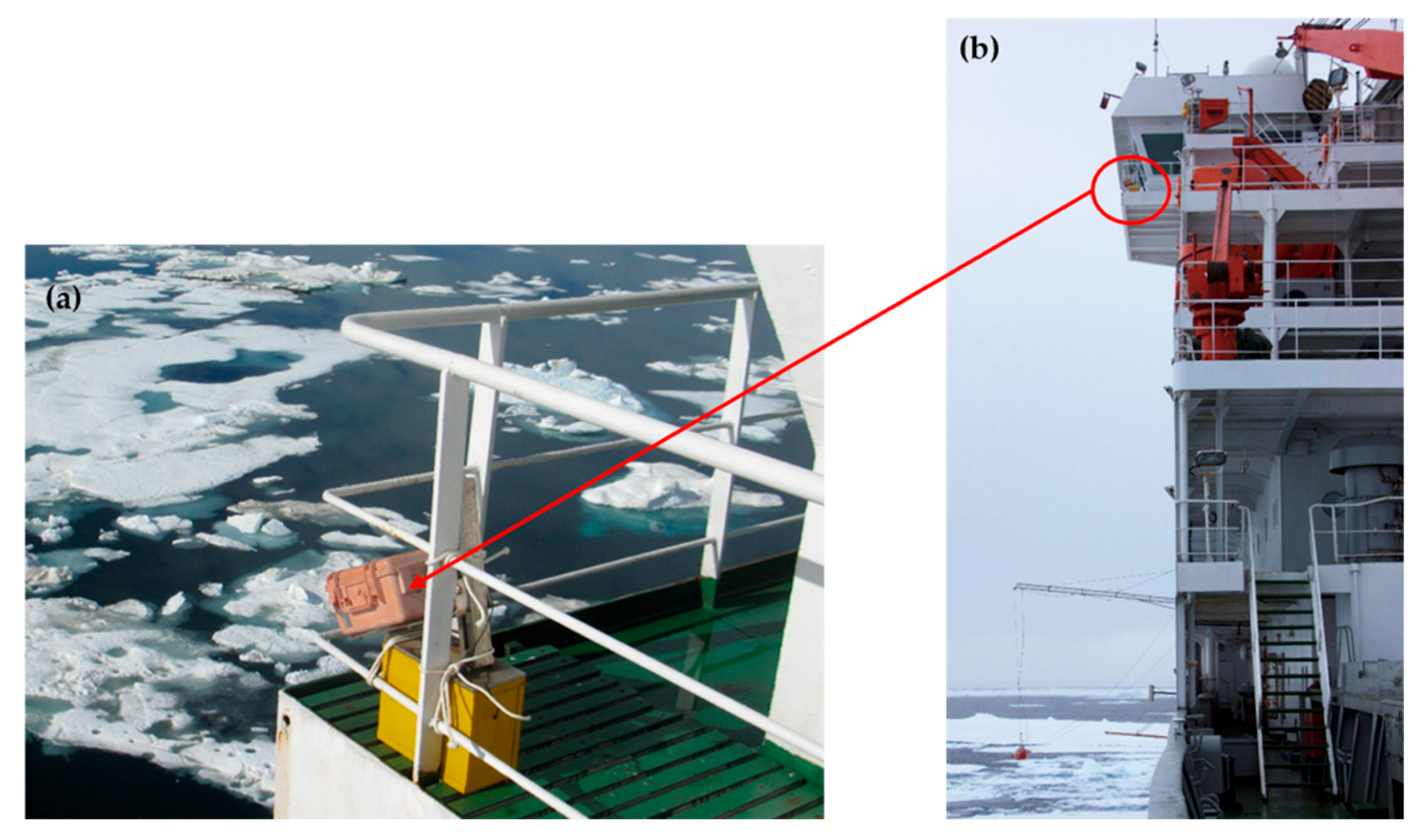
2.2. Shipborne Photographic Observations
2.3. Passive Microwave Data
2.4. Auxiliary Data
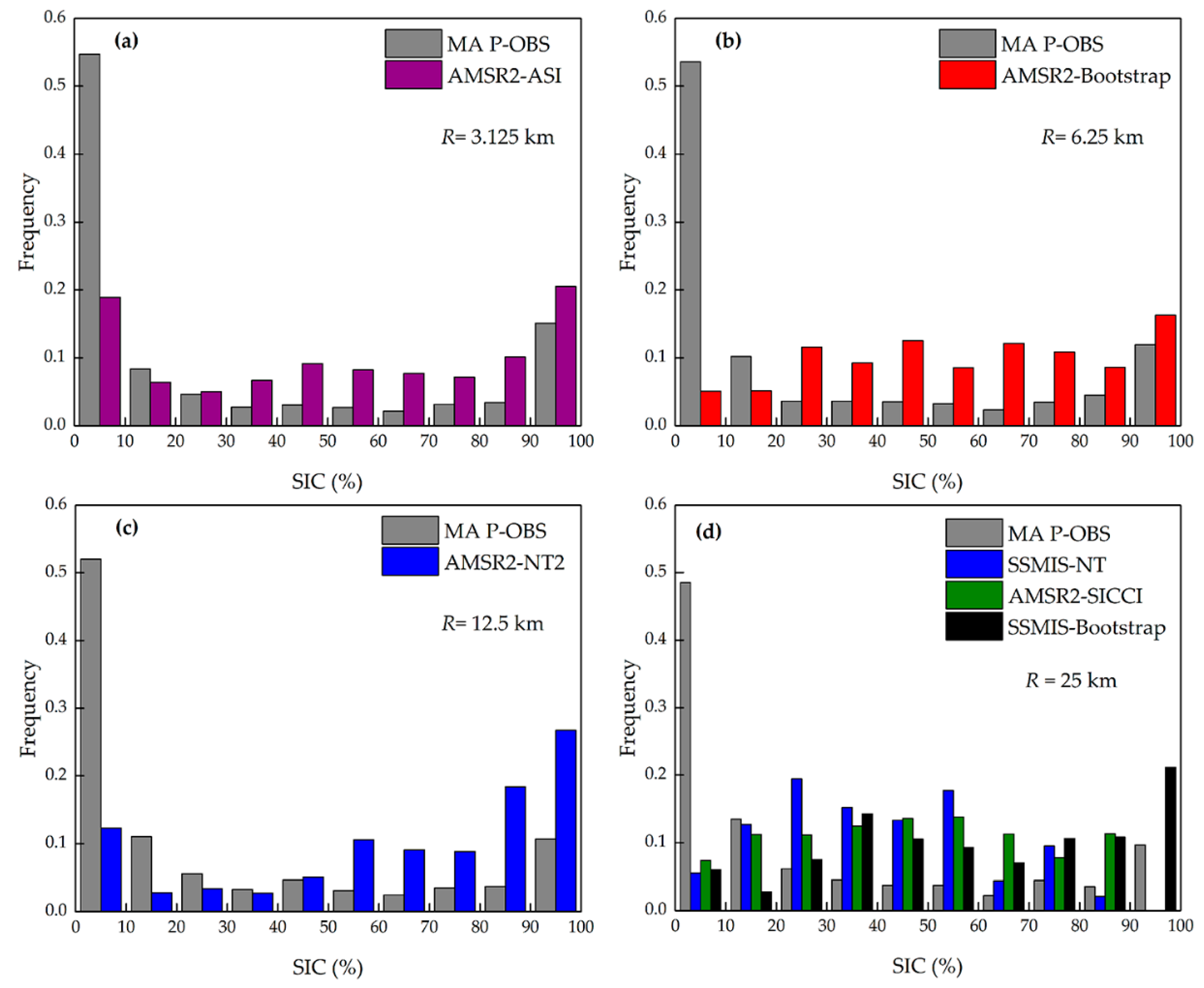
3. Results
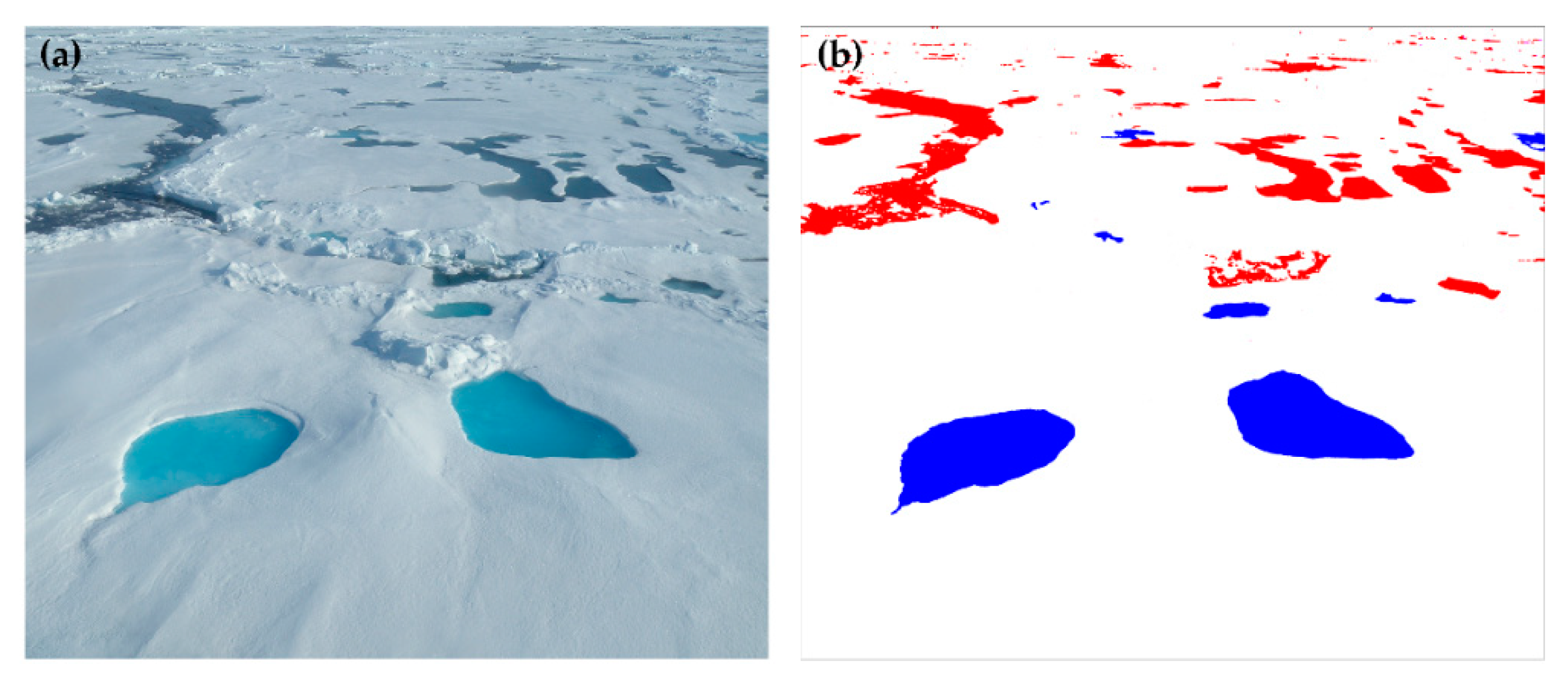
3.1. Sea Ice Concentration Derived from Shipborne Photographic Observations
3.2. Sea Surface Categories Distribution along the Cruise Path
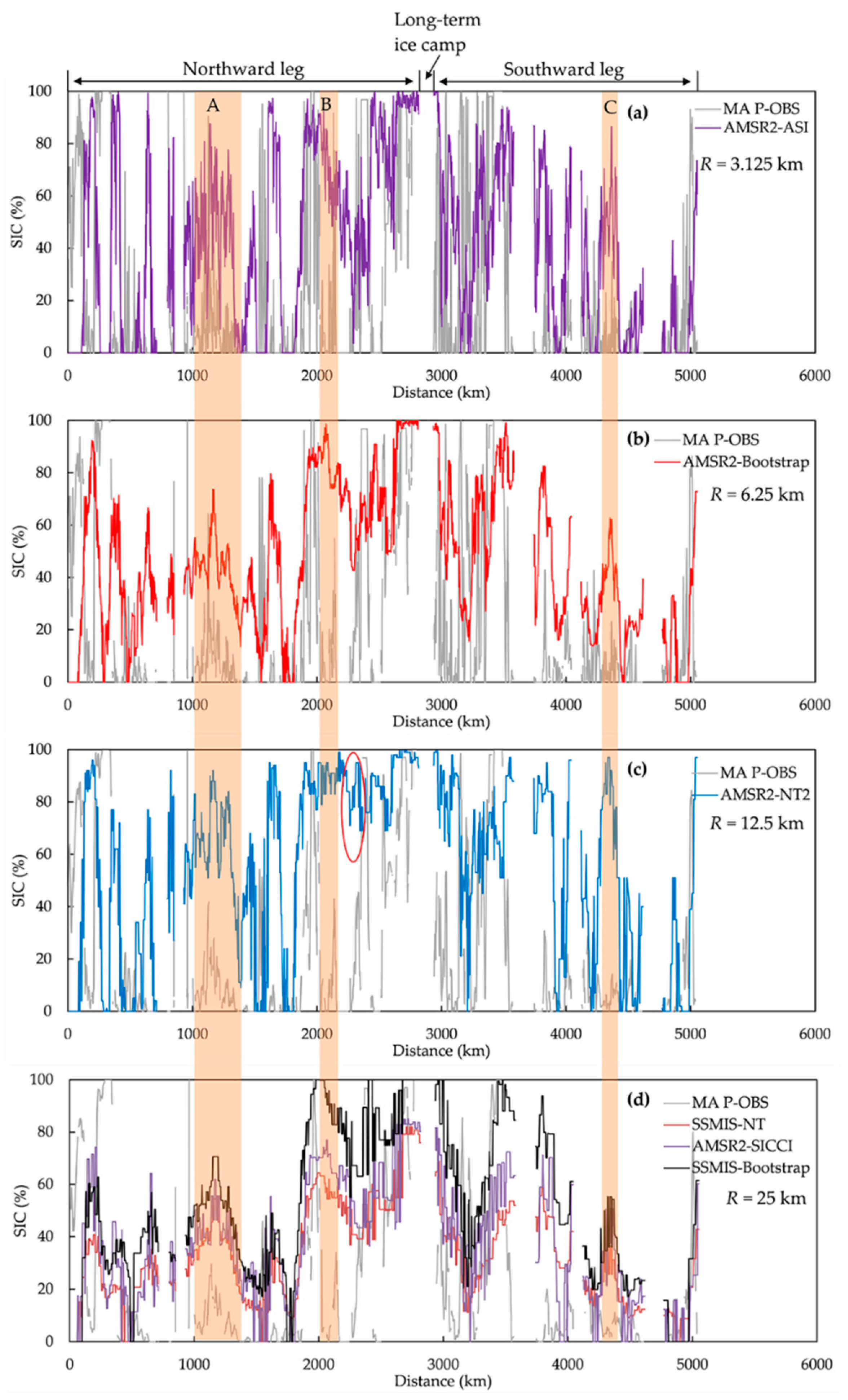
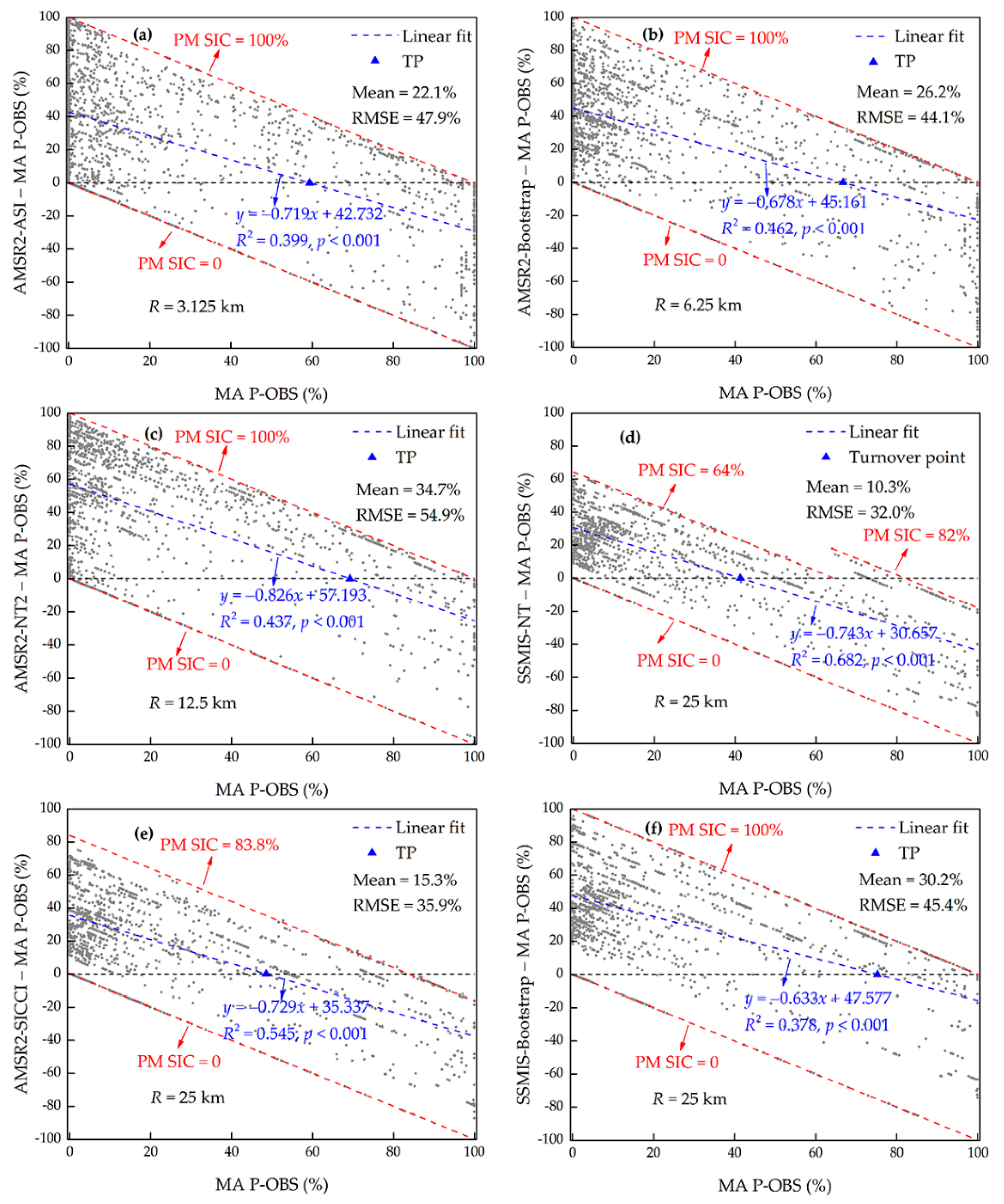
3.3. Comparison of Sea Ice Concentration Derived from Two Sources
4. Discussion
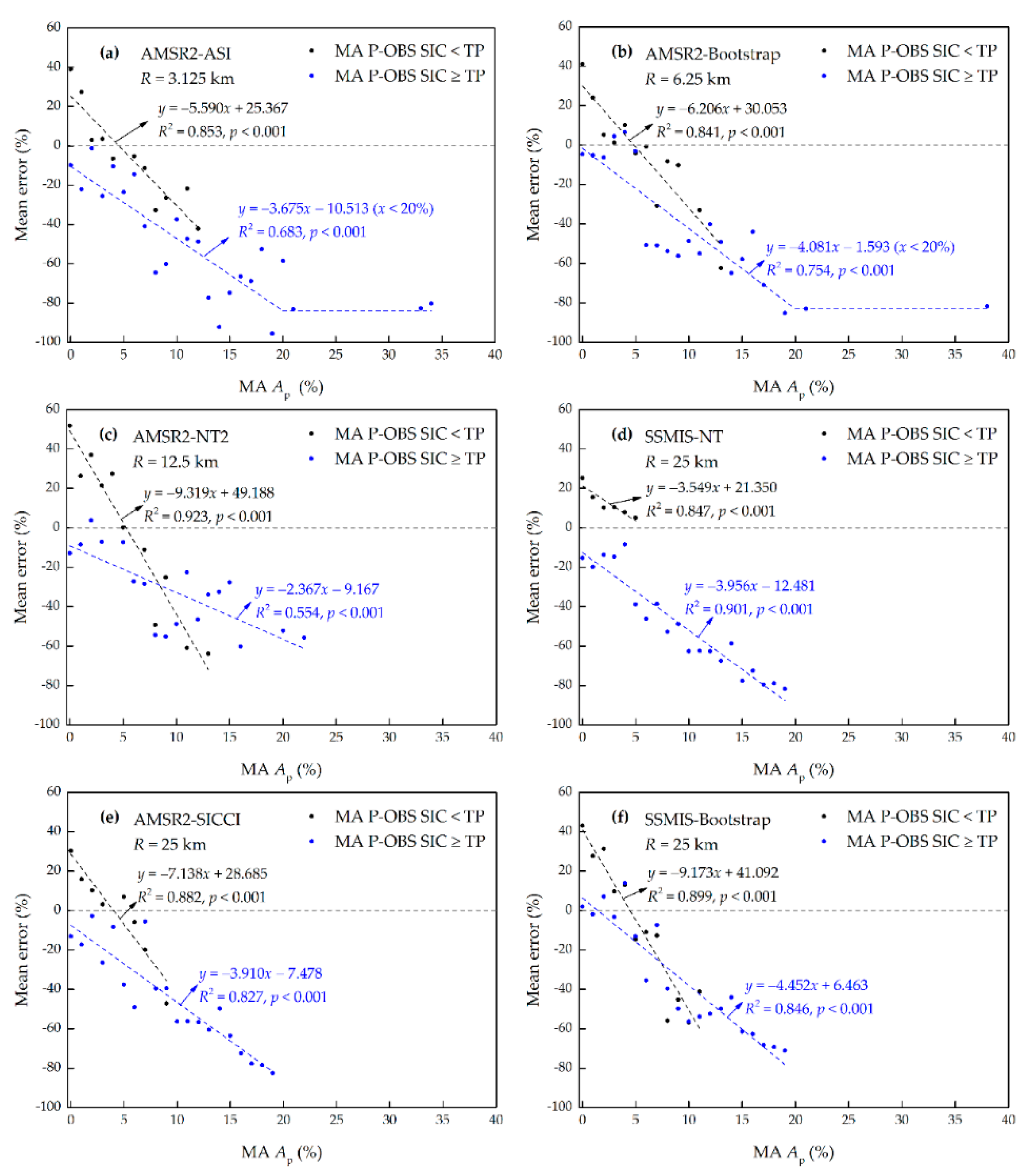
4.1. Factors Influencing the Difference of Sea Ice Concentration Derived from Two Sources
4.2. Melt Pond Effects on the Mean Error of Passive Microwave Sea Ice Concentration
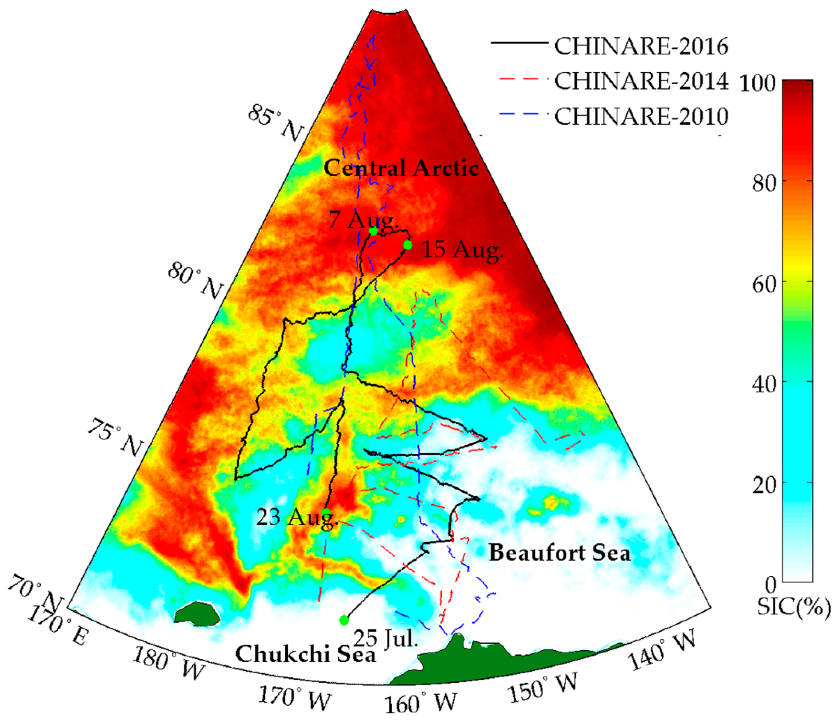
4.3. An Inter-Comparison of Sea Ice Concentration from 2010 to 2016
5. Conclusions
Author Contributions
Funding
Acknowledgments
Conflicts of Interest
References
- Renner, A.H.H.; Gerland, S.; Haas, C.; Spreen, G.; Beckers, J.F.; Hansen, E.; Nicolaus, M.; Goodwin, H. Evidence of Arctic sea ice thinning from direct observations. Geophys. Res. Lett. 2014, 41, 5029–5036. [Google Scholar] [CrossRef] [Green Version]
- Lindsay, R.; Schweiger, A. Arctic sea ice thickness loss determined using subsurface, aircraft, and satellite observations. Cryosphere 2015, 9, 269–283. [Google Scholar] [CrossRef] [Green Version]
- Comiso, J.C.; Parkinson, C.L.; Gersten, R.; Stock, L. Accelerated decline in the Arctic sea ice cover. Geophys. Res. Lett. 2008, 35, L01703. [Google Scholar] [CrossRef]
- Stroeve, J.C.; Kattsov, V.; Barrett, A.; Serreze, M.; Pavlova, T.; Holland, M.; Meier, W.N. Trends in Arctic sea ice extent from CMIP5, CMIP3 and observations. Geophys. Res. Lett. 2012, 39, L16502. [Google Scholar] [CrossRef]
- Laxon, S.W.; Giles, K.A.; Ridout, A.L.; Wingham, D.J.; Willatt, R.; Cullen, R.; Kwok, R.; Schweiger, A.; Zhang, J.; Haas, C.; et al. CryoSat-2 estimates of Arctic sea ice thickness and volume. Geophys. Res. Lett. 2013, 40, 732–737. [Google Scholar] [CrossRef] [Green Version]
- Kwok, R.; Cunningham, G.F. Contribution of melt in the Beaufort Sea to the decline in Arctic multiyear sea ice coverage: 1993−2009. Geophys. Res. Lett. 2010, 37, 79–93. [Google Scholar] [CrossRef]
- Comiso, J.C. Large decadal decline of the Arctic multiyear ice cover. J. Clim. 2012, 25, 1176–1193. [Google Scholar] [CrossRef]
- Deser, C.; Teng, H. Evolution of Arctic sea ice concentration trends and the role of atmospheric circulation forcing, 1979–2007. Geophys. Res. Lett. 2008, 35, L02504. [Google Scholar] [CrossRef]
- Lei, R.; Xie, H.; Wang, J.; Leppäranta, M.; Jónsdóttir, I.; Zhang, Z. Changes in sea ice conditions along the Arctic Northeast Passage from 1979 to 2012. Cold Reg. Sci. Technol. 2015, 119, 132–144. [Google Scholar] [CrossRef]
- Zhou, C.; Zhang, T.; Zheng, L. The characteristics of surface albedo change trends over the Antarctic sea ice region during recent decades. Remote Sens. 2019, 11, 821. [Google Scholar] [CrossRef]
- Serreze, M.C.; Barry, R.G. Processes and impacts of Arctic amplification: A research synthesis. Glob. Planet. Chang. 2011, 77, 85–96. [Google Scholar] [CrossRef]
- Takimoto, T.; Kanada, S.; Shimoda, H.; Wako, D.; Uto, S.; Izumiyama, K. Field measurements of local ice load on a ship hull in pack ice of the southern Sea of Okhotsk. In Proceedings of the OCEANS 2008-MTS/IEEE Kobe Techno-Ocean, Kobe, Japan, 8–11 April 2008. [Google Scholar]
- Langlois, A.; Barber, D.G.; Hwang, B.J. Development of a winter snow water equivalent algorithm using in situ passive microwave radiometry over snow-covered first-year sea ice. Remote Sens. Environ. 2007, 106, 75–88. [Google Scholar] [CrossRef]
- Langlois, A.; Barber, D.G. Advances in seasonal snow water equivalent (SWE) retrieval using in situ passive microwave measurements over first-year sea ice. Int. J. Remote Sens. 2008, 29, 4781–4802. [Google Scholar] [CrossRef]
- Kim, J.; Kim, K.; Cho, J.; Kang, Y.; Yoon, H.; Lee, Y. Satellite-based prediction of Arctic sea ice concentration using a deep neural network with multi-model ensemble. Remote Sens. 2019, 11, 19. [Google Scholar] [CrossRef]
- Strong, C.; Golden, K. Filling the polar data gap in sea ice concentration fields using partial differential equations. Remote Sens. 2016, 8, 442. [Google Scholar] [CrossRef]
- Comiso, J.C.; Meier, W.N.; Gersten, R. Variability and trends in the Arctic sea ice cover: Results from different techniques. J. Geophys. Res. Oceans 2017, 122, 6883–6900. [Google Scholar] [CrossRef]
- Spreen, G.; Kaleschke, L.; Heygster, G. Sea ice remote sensing using AMSR-E 89-GHz channels. J. Geophys. Res. 2008, 113, C02S03. [Google Scholar] [CrossRef]
- Beitsch, A.; Kern, S.; Kaleschke, L. Comparison of SSM/I and AMSR-E sea ice concentrations with ASPeCt ship observations around Antarctica. IEEE Trans. Geosci. Remote Sens. 2015, 53, 1985–1996. [Google Scholar] [CrossRef]
- Rees, G. Remote Sensing of Snow and Ice; Taylor & Francis: London, UK, 2006. [Google Scholar]
- Ivanova, N.; Pedersen, L.T.; Tonboe, R.T.; Kern, S.; Heygster, G.; Lavergne, T.; Sørensen, A.; Saldo, R.; Dybkjær, G.; Brucker, L.; et al. Inter-comparison and evaluation of sea ice algorithms: Towards further identification of challenges and optimal approach using passive microwave observations. Cryosphere 2015, 9, 1797–1817. [Google Scholar] [CrossRef]
- Andersen, S.; Tonboe, R.; Kern, S.; Schyberg, H. Improved retrieval of sea ice total concentration from spaceborne passive microwave observations using numerical weather prediction model fields: An intercomparison of nine algorithms. Remote Sens. Environ. 2006, 104, 374–392. [Google Scholar] [CrossRef]
- Comiso, J.C.; Cavalieri, D.J.; Parkinson, C.L.; Per, G. Passive microwave algorithms for sea ice concentration: A comparison of two techniques. Remote Sens. Environ. 1997, 60, 357–384. [Google Scholar] [CrossRef]
- Heygster, G.; Wiebe, H.; Spreen, G.; Kaleschke, L. AMSR-E geolocation and validation of sea ice concentrations based on 89 GHz data. J. Remote Sens. Soc. Jpn. 2009, 29, 226–235. [Google Scholar]
- Ivanova, N.; Johannessen, O.M.; Pedersen, L.T.; Tonboe, R.T. Retrieval of Arctic sea ice parameters by satellite passive microwave sensors: A comparison of eleven sea ice concentration algorithms. IEEE Trans. Geosci. Remote Sens. 2014, 52, 7233–7246. [Google Scholar] [CrossRef]
- Worby, A.P.; Allison, I. A technique for making ship-based observations of Antarctic sea ice thickness and characteristics, Part I: Observational techniques and results. In Antarctic CRC Research Report; Antarctic CRC: Hobart, Australia, 1999; Volume 14, pp. 1–23. [Google Scholar]
- Knuth, M.A.; Ackley, S.F. Summer and early-fall sea-ice concentration in the Ross Sea: Comparison of in situ ASPeCt observations and satellite passive microwave estimates. Ann. Glaciol. 2006, 44, 303–309. [Google Scholar] [CrossRef]
- Lei, R.; Li, Z.; Li, N.; Lu, P.; Cheng, B. Crucial physical characteristics of sea ice in the Arctic section of 143°−180°W during August and early September 2008. Acta Oceanol. Sin. 2012, 31, 65–75. [Google Scholar] [CrossRef]
- Lei, R.; Tian-Kunze, X.; Li, B.; Heil, P.; Wang, J.; Zeng, J.; Tian, Z. Characterization of summer Arctic sea ice morphology in the 135°−175°W sector using multi-scale methods. Cold Reg. Sci. Technol. 2017, 133, 108–120. [Google Scholar] [CrossRef]
- Xie, H.; Lei, R.; Ke, C.; Wang, H.; Li, Z.; Zhao, J.; Ackley, S.F. Summer sea ice characteristics and morphology in the Pacific Arctic sector as observed during the CHINARE 2010 cruise. Cryosphere 2013, 7, 1057–1072. [Google Scholar] [CrossRef] [Green Version]
- Ozsoy-Cicek, B.; Ackley, S.F.; Worby, A.; Xie, H.; Lieser, J. Antarctic sea-ice extents and concentrations: Comparison of satellite and ship measurements from International Polar Year cruises. Ann. Glaciol. 2011, 52, 318–326. [Google Scholar] [CrossRef]
- Pang, X.; Pu, J.; Zhao, X.; Ji, Q.; Qu, M.; Cheng, Z. Comparison between AMSR2 sea ice concentration products and pseudo-ship observations of the Arctic and Antarctic sea ice edge on cloud-free days. Remote Sens. 2018, 10, 317. [Google Scholar] [CrossRef]
- Worby, A.P.; Comiso, J.C. Studies of the Antarctic sea ice edge and ice extent from satellite and ship observations. Remote Sens. Environ. 2004, 92, 98–111. [Google Scholar] [CrossRef]
- Hall, R.J.; Hughes, N.; Wadhams, P. A systematic method of obtaining ice concentration measurements from ship-based observations. Cold Reg. Sci. Technol. 2002, 34, 97–102. [Google Scholar] [CrossRef]
- Perovich, D.K.; Tucker, W.B., III; Ligett, K.A. Aerial observations of the evolution of ice surface conditions during summer. J. Geophys. Res. 2002, 107. [Google Scholar] [CrossRef]
- Inoue, J.; Curry, J.A.; Maslanik, J.A. Application of Aerosondes to melt-pond observations over Arctic sea ice. J. Atmos. Ocean. Technol. 2008, 25, 327–334. [Google Scholar] [CrossRef]
- Lu, P.; Li, Z.; Cheng, B.; Lei, R.; Zhang, R. Sea ice surface features in Arctic summer 2008: Aerial observations. Remote Sens. Environ. 2010, 114, 693–699. [Google Scholar] [CrossRef]
- Weissling, B.; Ackley, S.; Wagner, P.; Xie, H. EISCAM—Digital image acquisition and processing for sea ice parameters from ships. Cold Reg. Sci. Technol. 2009, 57, 49–60. [Google Scholar] [CrossRef]
- Lu, W.; Zhang, Q.; Lubbad, R.; Loset, S.; Skjetne, R. A shipborne measurement system to acquire sea ice thickness and concentration at engineering scale. In Proceedings of the Arctic Technology Conference, St. John’s, NL, Canada, 24–26 October 2016. [Google Scholar]
- Lu, P.; Li, Z. A method of obtaining ice concentration and floe size from shipboard oblique sea ice images. IEEE Trans. Geosci. Remote Sens. 2010, 48, 2771–2780. [Google Scholar] [CrossRef]
- Worby, A.P.; Geiger, C.A.; Paget, M.J.; Van Woert, M.L.; Ackley, S.F.; DeLiberty, T.L. Thickness distribution of Antarctic sea ice. J. Geophys. Res. 2008, 113. [Google Scholar] [CrossRef] [Green Version]
- Alekseeva, T.A.; Frolov, S.V. Comparative analysis of satellite and shipborne data on ice cover in the Russian Arctic seas. Izv. Atmos. Ocean. Phys. 2013, 49, 879–885. [Google Scholar] [CrossRef]
- Wang, Q.; Li, Z.; Lu, P.; Lei, R.; Cheng, B. 2014 summer Arctic sea ice thickness and concentration from shipborne observations. Int. J. Digit. Earth 2018, 1–17. [Google Scholar] [CrossRef]
- Mcgovern, D.J.; Bai, W. Experimental study on kinematics of sea ice floes in regular waves. Cold Reg. Sci. Technol. 2014, 103, 15–30. [Google Scholar] [CrossRef]
- Huang, W.; Lu, P.; Lei, R.; Xie, H.; Li, Z. Melt pond distribution and geometry in high Arctic sea ice derived from aerial investigations. Ann. Glaciol. 2016, 57, 105–118. [Google Scholar] [CrossRef] [Green Version]
- Li, L.; Ke, C.; Xie, H.; Lei, R.; Tao, A. Aerial observations of sea ice and melt ponds near the North Pole during CHINARE2010. Acta Oceanol. Sin. 2017, 36, 64–72. [Google Scholar] [CrossRef]
- Lu, P.; Leppäranta, M.; Cheng, B.; Li, Z.; Istomina, L.; Heygster, G. The color of melt ponds on Arctic sea ice. Cryosphere 2018, 12, 1331–1345. [Google Scholar] [CrossRef] [Green Version]
- Martin, T.; Augstein, E. Large-scale drift of Arctic Sea ice retrieved from passive microwave satellite data. J. Geophys. Res. Oceans 2000, 105, 8775–8788. [Google Scholar] [CrossRef] [Green Version]
- Sumata, H.; Kwok, R.; Gerdes, R.; Kauker, F.; Karcher, M. Uncertainty of Arctic summer ice drift assessed by high-resolution SAR data. J. Geophys. Res. Oceans 2015, 120, 5285–5301. [Google Scholar] [CrossRef] [Green Version]
- Leppäranta, M. The Drift of Sea Ice, 2nd ed.; Springer-Praxis: Heidelberg, Germany, 2011. [Google Scholar]
- Cavalieri, D.J.; Onstott, R.G.; Burns, B.A. Investigation of the effects of summer melt on the calculation of sea ice concentration using active and passive microwave data. J. Geophys. Res. 1990, 95, 5359–5369. [Google Scholar] [CrossRef]
- Comiso, J.C.; Kwok, R. Surface and radiative characteristics of the summer Arctic sea ice cover from multisensor satellite observations. J. Geophys. Res. 1996, 101, 28397–28416. [Google Scholar] [CrossRef]
- Kern, S.; Rösel, A.; Pedersen, L.T.; Ivanova, N.; Saldo, R.; Tonboe, R.T. The impact of melt ponds on summertime microwave brightness temperatures and sea-ice concentrations. Cryosphere 2016, 10, 2217–2239. [Google Scholar] [CrossRef] [Green Version]


| PM Sensor | Algorithm | Channels Used for Retrieval (GHz) | Resolution (km) |
|---|---|---|---|
| SSMIS | Bootstrap | 19.4 V 1, 37.0 V | 25 × 25 |
| NT | 19.4 V, 19.4 H, 37.0 V | 25 × 25 | |
| AMSR2 | ASI | 89.0 V, 89.0 H | 3.125 × 3.125 |
| Bootstrap | 18.7 V, 36.5 V | 6.25 × 6.25 | |
| NT2 | 18.7 V, 18.7 H, 36.5 V, 36.5 H, 89.0 V, 89.0 H | 12.5 × 12.5 | |
| SICCI | 18.7 V, 18.7 H, 36.5 V, 36.5 H | 25 × 25 |
| PM Algorithm | AMSR2-ASI | AMSR2-Bootstrap | AMSR2-NT2 | SSMIS-NT | AMSR2-SICCI | SSMIS-Bootstrap |
|---|---|---|---|---|---|---|
| TP (%) | 59.4 | 66.6 | 69.2 | 41.3 | 48.5 | 75.2 |
| PM Algorithm | <TP | ≥TP | ||
|---|---|---|---|---|
| Mean Error (%) | RMSE (%) | Mean Error (%) | RMSE (%) | |
| AMSR2-ASI | 36.5 | 49.1 | −23.6 | 42.8 |
| AMSR2-Bootstrap | 37.3 | 46.3 | −15.9 | 34.3 |
| AMSR2-NT2 | 46.9 | 58.0 | −19.5 | 38.0 |
| SSMIS-NT | 23.9 | 29.4 | −26.6 | 38.2 |
| AMSR2-SICCI | 27.8 | 35.7 | −24.5 | 36.5 |
| SSMIS-Bootstrap | 38.1 | 47.2 | −14.6 | 33.2 |
| Year | MIZ | PIZ | Chukchi Sea | Beaufort Sea | Central Arctic |
|---|---|---|---|---|---|
| 2010 | 30% | 66% (northward leg) 71% (southward leg) | / | / | / |
| 2014 | 48% | 76% | 56% | 59% | 98% |
| 2016 | 20% | 70% | 21% | 8% | 56% |
© 2019 by the authors. Licensee MDPI, Basel, Switzerland. This article is an open access article distributed under the terms and conditions of the Creative Commons Attribution (CC BY) license (http://creativecommons.org/licenses/by/4.0/).
Share and Cite
Wang, Q.; Lu, P.; Zu, Y.; Li, Z.; Leppäranta, M.; Zhang, G. Comparison of Passive Microwave Data with Shipborne Photographic Observations of Summer Sea Ice Concentration along an Arctic Cruise Path. Remote Sens. 2019, 11, 2009. https://doi.org/10.3390/rs11172009
Wang Q, Lu P, Zu Y, Li Z, Leppäranta M, Zhang G. Comparison of Passive Microwave Data with Shipborne Photographic Observations of Summer Sea Ice Concentration along an Arctic Cruise Path. Remote Sensing. 2019; 11(17):2009. https://doi.org/10.3390/rs11172009
Chicago/Turabian StyleWang, Qingkai, Peng Lu, Yongheng Zu, Zhijun Li, Matti Leppäranta, and Guiyong Zhang. 2019. "Comparison of Passive Microwave Data with Shipborne Photographic Observations of Summer Sea Ice Concentration along an Arctic Cruise Path" Remote Sensing 11, no. 17: 2009. https://doi.org/10.3390/rs11172009