Development of a Parameterized Model to Estimate Microwave Radiation Response Depth of Frozen Soil


1
Land Satellite Remote Sensing Application Center, Ministry of Natural Resources of the People’s Republic of China, Beijing 100048, China
2
State Key Laboratory of Remote Sensing Science, Jointly Sponsored by Beijing Normal University and Institute of Remote Sensing and Digital Earth of Chinese Academy of Sciences, Beijing Engineering Research Center for Global Land Remote Sensing Products, Faculty of Geographical Science, Beijing Normal University, Beijing 100875, China
3
State Key Laboratory of Earth Surface Processes and Resource Ecology, Faculty of Geographical Science, Beijing Normal University, Beijing 100875, China
4
School of Urban Construction, Beijing City University, Beijing 100083, China
*
Author to whom correspondence should be addressed.
Remote Sens. 2019, 11(17), 2028; https://doi.org/10.3390/rs11172028
Submission received: 22 July 2019
/
Revised: 19 August 2019
/
Accepted: 26 August 2019
/
Published: 28 August 2019
(This article belongs to the Special Issue Remote Sensing of Environmental Changes in Cold Regions)
Abstract
:The sensing depth of passive microwave remote sensing is a significant factor in quantitative frozen soil studies. In this paper, a microwave radiation response depth (MRRD) was proposed to describe the source of the main signals of passive microwave remote sensing. The main goal of this research was to develop a simple and accurate parameterized model for estimating the MRRD of frozen soil. A theoretical model was introduced first to describe the emission characteristics of a three-layer case, which incorporates multiple reflections at the two boundaries. Based on radiative transfer theory, the total emission of the three layers was calculated. A sensitivity analysis was then performed to demonstrate the effects of soil properties and frequency on the MRRD based on a simulation database comprising a wide range of soil characteristics and frequencies. Sensitivity analysis indicated that soil temperature, soil texture, and frequencies are three of the primary variables affecting MRRD, and a definite empirical relationship existed between the three parameters and the MRRD. Thus, a parameterized model for estimating MRRD was developed based on the sensitivity analysis results. A controlled field experiment using a truck-mounted multi-frequency microwave radiometer (TMMR) was designed and performed to validate the emission model of the soil freeze–thaw cycle and the parameterized model of MRRD developed in this work. The results indicated that the developed parameterized model offers a relatively accurate and simple way of estimating the MRRD. The total root mean square error (RMSE) between the calculated and measured MRRD of frozen loam soil was approximately 0.5 cm for the TMMR’s four frequencies.
1. Introduction
Permafrost and seasonally frozen soil, whose thermal and physical properties differ from unfrozen soil, are key components of the cryosphere. The regional energy and water balance are dramatically modified by the phase transition of soil water during the freeze–thaw process. The freezing–thawing of soil induced the release of decomposable organic carbon, and thus had a profound influence on the overall functioning of ecosystems [1]. However, the degradation of permafrost, which releases latent heat and carbon, has become a positive global warming feedback [2]. Previous experiments have shown that the carbon emission in soil profile varied spatially and temporally and was correlated with soil frozen depth [3]. Hence, it is necessary to determine the soil frozen depth for a given frozen area and explore the extent and distribution of frozen areas.
Satellite remote-sensing technology is an ideal tool for obtaining the spatial and temporal information of frozen areas. Passive microwave remote sensing has been used to provide qualitative information in previous studies because of less vulnerably linked to cloud cover and more frequent revisit time comparing to optical remote sensing. In some previous research, many scientists have devoted to exploring freeze/thaw discrimination methods using passive microwave remote sensing data [4,5,6,7,8]. Recently, multiple studies have focused on the quantitative frozen ground remote sensing, such as the amount of water released by the phase transition during the freeze/thaw process, the frost penetration velocity [9,10], and so on. It should be noted that in these investigations, land surface properties were monitored using microwave remote-sensing sensors, which provided an integrated microwave emission signal over a certain surface within a certain depth. Knowing this depth is important for this research referred to above. It is an indication of the thickness of the surface layer, within which variations in soil moisture or other soil parameters can significantly affect the emitted radiation at a certain frequency [11,12]. For different frequencies, the depth varies too. Hence, it can be an explanation for some phenomenon in freeze–thaw related research because signals from different surfaces might indicate different depth. In addition, it is useful for planning ground data collection campaigns for model and algorithm development and validation in this field.
However, what the definition of this ‘depth’ is and how deep the ‘depth’ refers to are two main issues in front of us. Many scientists attempt to answer these two questions and have contributed to some related work. Ulaby proposed a penetration depth model for active microwaves [13]. It might cause errors for the active microwave model to be used in passive microwave remote sensing applications because of the disparate working mechanisms between active and passive microwave remote sensing [14]. Wilheit proposed a thermal sampling depth and reflectivity sampling depth based on a multiple-layered and coherent radiative transfer model [15]. The thermal sampling depth is the depth at which thermal radiation upwelling originates in the soil and the reflectivity sampling depth was determined as the depth at which the isothermal and non-isothermal reflectivities were equal. The reflectivity characteristics changed over the depth of approximately 1/10–1/7 of the wavelengths in the medium, and the thermal radiation was generally larger [16]. Blinn and Paloscia gave a feasible way to study the question regarding which depth of soil is responsible for the greatest part of the emission upwelling from soil by conducting a controlled ground experiment [17,18]. The conclusion of the sensitivity of L band emission to the moisture content of a soil layer about 5 cm thick was confirmed. There are also several theoretical and experimental results that demonstrated that the sensing depths were approximately 2–20 cm for different soil conditions at L band [12,19,20,21,22] and about 2 cm at 5 GHz with a soil moisture of 0.1 cm3/cm3 [20].
Although, previous studies have revealed different definitions and results of the passive microwave remote-sensing depth, a feasible method to estimate a depth that determined as the source of the predominant microwave remote-sensing signals has been poorly investigated. As a result, scientists commonly use an empirical depth. For example, although the depth varies with frequency and soil characteristics, soil moisture measurements with depths of at least 0–5 cm are widely used to validate remote-sensing data at L band [23,24,25]. It is possible that for unfrozen soil the measurements of soil moisture are only partially representative of average values measured by a radiometer. Finally, it can be seen that most of the research referred to unfrozen soil. As the dielectric and microwave radiation characteristics of unfrozen soil are quite different with that of frozen soil [26,27,28], the models of estimating penetration depth for unfrozen soil usually do not work well for frozen soil.
In this research, we will try to propose a passive microwave remote-sensing response depth (MRRD) and develop a simple parameterized model to determine its value for frozen soil. A field experiment using a truck-mounted multi-frequency microwave radiometer (TMMR) will be introduced in Section 2.1. Field experiment data will be used for validation. In Section 2.2, we propose the theory used to investigate the passive microwave remote sensing response depth and develop a parameterized model to estimate the frozen soil response depth. The measurements are analyzed and discussed in Section 3 and Section 4. In Section 5 we give the conclusions of this study.
2. Materials and Methods
2.1. Field Experiment
As has already been done by other investigators [17,18], we carried out a “microwave radiation response depth experiment” by putting soil samples over a metal plate. A TMMR was used to measure the microwave radiation from an aluminum sheet covered with soil samples of various thicknesses. The controlled experiment data is used to investigate the effects of frequency and soil parameters on the microwave remote sensing response depth and validated a parameterized model of the microwave radiation response depth (MRRD) in frozen soil. The detailed field experiment is presented in the following sections.
2.1.1. Experimental Setup and Material Preparation
The experiment was performed in Baoding, Hebei Province, China (38°42’10.21’’N, 115°23’18.23’’E) from 12 to 19 January 2012. During this period, the soil typically froze at night and thawed during the day. The most important instrument in this experiment is the TMMR. It is an eight-channel radiometer with four frequencies (6.925, 10.65, 18.7, and 36.5 GHz), with vertical and horizontal polarization at each frequency. The TMMR can collect data at multiple angles, both in the zenith (from −90° to 90°) and azimuthal directions (from 0° to 360°). The TMMR was calibrated on a four-point calibration scheme before the experiment, and the precision of measurements was also tested by measuring a calm water area. An absolute Tb accuracy of 1 K could be achieved with the accuracy of calibration target temperature sensors and the minimization of thermal gradients. Detailed calibration and test procedures were described in [29].
The radiometer was placed on a truck using a hydraulic lifting platform, which lifted the apparatus to 4.78 m above the ground. Figure 1 presents the observation field. Measurements were made toward the south to avoid the shadow of the truck. The incident angle was fixed at 45° during the whole experiment. The −10 dB footprints of the four antennas were calculated and labeled on the ground according to the radiometer configuration. Due to the low emissivity of aluminum, aluminum sheets were used as the background for the following measurements. Eight aluminum sheets (each 1 m × 2 m) were arranged on the ground in two rows to form a 4 m × 4 m mosaic, which completely covered the four antenna footprints. This can ensure that the signals received by TMMR are from the objects on the aluminum sheets. The soil was air dried and sieved to ensure a homogeneous soil moisture and texture.
For each thickness, the appropriate amount of water was mixed with the dried soil to obtain the desired soil moisture. The mixture was used to cover the aluminum sheets, and the layer was artificially smoothed. To improve soil plasticity and artificially smooth the soil surface, appropriate soil moisture content is needed. Note that covering the eight aluminum sheets with the area of 16 m2 using the mixture and artificially smoothing the sample surface is a very time-consuming and labor-intensive process. In addition, a heterogeneous soil temperature profile may exist if the soil thickness is too large. Conversely, soil samples with thin thickness are more easily to be freeze uniformly. Thus, only five and relatively thin soil samples were analyzed in this experiment.
2.1.2. Measurements
The TMMR was used to measure the microwave radiation from the aluminum sheet to obtain the emissivity at four frequencies. During the experiment, the brightness temperature of the aluminum sheet, which was covered by various soil layer thicknesses, was measured using a TMMR. To eliminate the atmospheric effect on each measurement, the atmospheric downward radiations in different frequencies were measured by TMMR and then were used to calculate the emissivity values of soil samples.
In this experiment, the initial soil moisture of soil sample is 0.433 cm3/cm3, and the thicknesses of five soil samples were 0.18, 0.43, 0.63, 0.96, and 1.06 cm, respectively. The continuous measurements of each sample lasted for approximately 24 hours to include the typical thawing and freezing processes that occur during the day and night, respectively. Because the physical temperature remained too high for completely freezing during the first 24-hour period, the 1.06 cm soil sample was observed for about two days. To avoid soil moisture evaporation, a plastic film was used to cover the soil. A trial conducted before our experiment revealed that the effect of the plastic film was negligible. The soil temperature and moisture were automatically measured every 3 minutes by the temperature and moisture sensors and collected using an Intelligent Data Acquisition Collector (IDAC) (Figure 1). As one thickness measurement was being conducted, another sample was being prepared. The thickness of the soil sample was measured after one sample observation was performed.
A cutting ring was used to measure the soil bulk density. The mean bulk density was 1.41 g/cm3. The soil texture is classified as loam (sand: 30.16%, silt: 48.85%, clay: 20.99%) according to the U.S. Department of Agriculture classification scheme.
2.2. Methodology
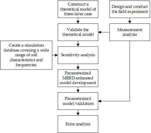
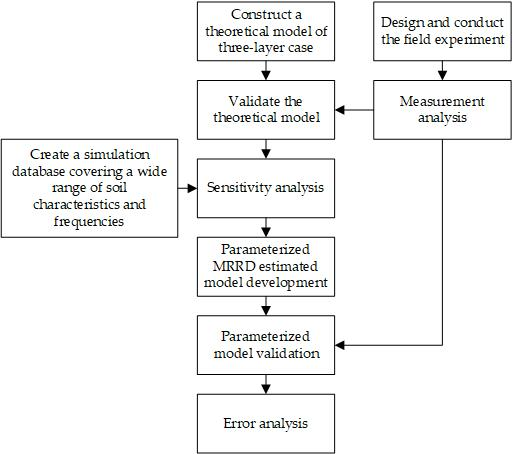
To develop a parameterized model to estimate MRRD of frozen soil, the definitions of the MRRD and the theoretical model utilized were introduced firstly. Sensitivity analysis were then performed to determine the relationship between MRRD and soil parameters using the theoretical model. The parameterized model was developed based on sensitivity analysis results. The field experiment data introduced in 2.1 were used for validation of theorical model and parameterized model. A flow chart has shown the parameterized model development and validation process (Figure 2).
2.2.1. Microwave Radiation Response Depth (MRRD)
To describe the characteristics observed by passive microwave remote sensing, the MRRD was defined in this paper. We used the following experiment to obtain an expression for the MRRD. A radiometer was used to measure the emissivity of aluminum sheets (theoretically, its emissivity is 0 and reflectivity is 1.0) covered with various soil thicknesses. As a result, when the soil layer was thin, the brightness temperature measured by the radiometer was very low. The observed brightness temperature increased as the soil thickness increased, and it will stabilize when the soil thickness increases. Because the emissivity can be deduced by normalizing brightness temperature to a physical temperature of the target, herein, the emissivity was used to describe the definition of MRRD. If the observed emissivity reaches , i.e., achieves stability, the MRRD can be defined as the depth at which:
Where, is the emissivity of soil with thickness of z. The above formula indicates that at depth z, the difference between the emissivity and the maximum emissivity (the stable value) is only 0.001 (approximately 0.1–0.3 K for frozen soil). This depth is defined as the MRRD. The MRRD provides a reference for the primary source of the observed signals.
2.2.2. Theoretical Model
A three-layer case was used to illustrate the theoretical model for frozen/thaw soil (Figure 3). We define the air, soil, and aluminum sheet as the first, second, and third layers and the air–soil and soil–aluminum sheet boundaries as the first and second boundaries, respectively.
The model was used to calculate emissions using the radiative transfer theory [13]. It is a non-coherent model, which does not include interference. The brightness temperature consists of two contributions:
where and are the brightness temperature contributions due to the layer 2 and 3 emissions, respectively. is the angle of the radiation emitted into layer 1.
Multiple reflections at the two boundaries were incorporated into this model. Each of the two bottom layers is assumed to isotropically radiate, and the boundary roughness is ignored. We are only interested in the radiation that is emitted into layer 1 at an angle of . The only radiation of interest in layer 2 is that emitted at boundary 1 at an angle of . This consists of upward emissions and downward emissions that are reflected by boundary 2 toward boundary 1. The contributions of these two components to can be designated by the upward emission, , and downward emission, :
Consider a thin horizontal stratum in layer 2 at a depth of ζ and a thickness of dζ. In the upward direction, this stratum’s emissions are first attenuated by the stratum at depth ζ and boundary 1 along the path. Then, at boundary 1, a fraction of this attenuated emission is transmitted across the boundary and the remainder is reflected. The reflected portion decreases as it travels to boundary 2. It is then partially reflected toward boundary 1 and partially transmitted into layer 3. This process will infinitely continue. In the downward direction, this stratum’s emissions are also attenuated by the stratum at depth ζ and boundary 2 along the path. A fraction is transmitted across boundary 2, while the remainder is reflected. It then experiences the same reflections between boundaries 1 and 2 as the upward emission. The total energy can be found by integrating over the 0 to d depth range.
For layer 3, the upwelling emission at angle is transmitted by boundary 2 and attenuated by layer 2, then reflected toward boundary 1, which is the only component we consider. It can be computed in a similar manner as layer 2. The theoretical model can be described as:
The above expression gives the total brightness temperature, , of the three layers. In the model, Γ is the reflectivity of a boundary, and the subscripts 1 and 2 indicate boundaries 1 and 2. The reflectivity can be calculated using Fresnel’s law at the first boundary. T is the physical temperature of each layer. Subscripts 1, 2, and 3 indicate layers 1, 2, and 3, respectively. θ θand are the incident angle and polarization. L is the power loss factor, which can be expressed by:
where d is the soil thickness, is the real transmission angle, and is the extinction coefficient. If soil medium scattering is ignored, is approximately equal to the absorption coefficient, , given by:
where is the wavelength in free space and is the corresponding permittivity of soil.
The low emissivity of the aluminum sheet makes it an ideal background material. Additionally, it can shield signals from below the aluminum sheet. We assume that the soil properties are uniform with depth, the reflectivity of the aluminum sheet is 1.0 and the single scattering albedo is sufficiently small that diffuse scattering can be ignored (a = 0). The implications of these assumptions will be discussed in Section 4.
Because the physical characteristics of the soil layer are unknown, several empirical models were introduced. Unfrozen soil can be considered a mixture of air, solid soil, bound water, and free water. Dobson developed an empirical model to calculate the permittivity [30], which has been widely used in soil permittivity estimations.
Here, , , and are the dielectric constants of the unfrozen soil, solid soil, and free water, respectively. and are the bulk density and specific density in g/cm3, respectively. is the volumetric soil moisture in cm3/cm3. α is a constant shape factor, and β is a coefficient dependent on the soil textural composition.
Due to the adsorption forces and curvature at the soil particle surfaces in frozen soil, a certain amount of water remains unfrozen, even when the soil temperature is below 0 °C. This is called the unfrozen water content. The amount of unfrozen water mainly depends on the physical properties of the soil. Typically, the specific surface, which is the ratio of total surface area to the mass of the soil, controls the binding force on the water. The higher the soil specific surface area, the greater the binding force, making the water prone to remaining unfrozen. However, the unfrozen water content overcomes the adsorption forces of soil particles and freezes as the soil temperature continues to decrease. Anderson developed an empirical model for estimating the unfrozen water content using the soil temperature and specific surface area of the soil [31] which is given by:
where is the unfrozen water content (cm3/cm3), T is the soil temperature in Kelvin, and S is the soil specific area in m2/g, which is determined based on the particle-size distribution of the soil. The soil specific area can be predicted using an empirical model [32] based on the sand, silt, and clay contents:
The unfrozen water content directly affects the permittivity of the frozen soil due to the large difference in the permittivity between ice and water. Based on Dobson’s work, Zhang added a term to the parameterized model to describe the ice fraction contribution to the frozen soil permittivity [26]. This model can be used for various soil types and includes soil texture, bulk density, soil moisture, and temperature inputs. It has been used in previous passive microwave remote sensing studies of frozen soil [7,9]. The simulated results were also validated using experimental data obtained with an Agilent PNA Network Analyzer E8362B. The expression can be written as:
where the subscripts , , , , and refer to solid soil, ice, free water, volumetric unfrozen water, and the volumetric ice content, respectively.
2.2.3. Sensitivity Analysis
The attenuation of electromagnetic waves in the soil is determined based on the soil’s permittivity and the wavelength. Hence, the MRRD is mainly affected by the factors impact on the dielectric characteristics of the soil. A sensitivity analysis was conducted to determine the relationship between MRRD and soil parameters using the theoretical model described above. We have performed the comparison between MRRD computed using the theoretical model for horizontal and vertical polarization. It can be concluded that the MRRDs for horizontal and vertical polarization are highly correlated and have negligible difference when the incident angle equals zero. However, the MRRD for horizontal polarization was slightly higher than that for vertical polarization because different Fresnel reflectivity of polarizations exists at the air–soil boundary if the incident angle is not zero [12,33]. For simplicity, the vertical polarization brightness temperature is used in the following analysis. A simulation database covering a wide range of soil characteristics and frequencies was created. The unfrozen water content, soil temperature, frequency, bulk density, and soil specific surface area were selected as the factors to be analyzed. The key input parameters of the theoretical model are listed in Table 1. Note that the unfrozen water content was calculated by temperature and soil specific surface area using Equation (8). The incidence angle determines the microwave radiation path, which can be calculated with vertical path. Therefore, it was set to be 55° according to the commonly used Advanced Microwave Scanning Radiometer–Earth Observing System (AMSR-E) observation configuration.
To compare the sensitivity of soil characteristics and frequencies to MRRD, the normalized index for each parameter was used in the sensitivity analysis. The normalized index for a parameter can be expressed as
Where, indicates the values of soil temperature, frequency, soil specific surface area and bulk density. is the normalized value of these parameters. The subscript max and min are the maximum and minimum value of the corresponding parameters set in the simulation database.
As described above, not all of the liquid water transforms into ice when the temperature drops below 0 °C. The unfrozen water in the soil is determined based on the temperature and soil texture. Figure 4a–c show the dependence of the MRRD on temperature, soil specific area, and unfrozen soil water content, respectively. For a given frequency, the MRRD increases when the temperature varies from −2 °C to −30 °C and the soil specific surface area ranges from 253.042 to 37.442 m2/g. This can be explained by the positive correlation between the unfrozen water and temperature. The unfrozen water content in the frozen soil decreases as the temperature decreases, leading to a lower soil permittivity and weaker electromagnetic extinction when all other soil characteristics are held constant. Another parameter affecting the unfrozen water in the soil is the soil texture, which impacts the soil particle water adsorption. The higher the specific surface area, the stronger the water binding force, leading to more unfrozen water and a higher permittivity (Figure 4b). Figure 4d illustrates the MRRD decrease with increasing frequency (decreasing the wavelength). Additionally, at −15 °C, the difference in the MRRD is 2 cm (approximately 8 cm and 6 cm) for frequencies ranging from 6.925 GHz to 10.65 GHz, but only 0.4 cm (5.1 cm and 4.7 cm) for frequencies from 18 GHz to 36.5 GHz. The MRRD is weakly dependent on the frequency above 10 GHz. This behavior is clearly shown in Figure 4d and agrees with our expectations of the microwave remote sensing penetrability.
Overall, the MRRD is negatively correlated with all parameters. The sensitivity of MRRD to unfrozen water content, temperature, frequency, and soil specific surface area is larger than that to bulk density (Figure 4e). Furthermore, the bulk density generally relates to the composition of soil particles. Hence, it is not considered in the parameterized model development.
2.2.4. Parameterized MRRD Estimated Model Development
Based on the sensitivity analysis in part 2.2.3, we concluded that the observation frequency, unfrozen water content, temperature, and specific surface area are important factors for determining the frozen soil MRRD. Note that the measurements of unfrozen water content in frozen soil is generally very complicated and difficult. Furthermore, the unfrozen water content was represented by temperature and soil specific surface area. Therefore, it was not included in the parameterized model development. Hence, three parameters, including temperature, frequency, and specific surface area, were used to develop a simple, accurate model to estimate the MRRD in this research. The relationship between the temperature and MRRD was analyzed firstly based on the simulation database as shown in Figure 5.
The relationship between the MRRD and temperature can be expressed by the exponential function:
where is the MRRD in cm and T is the physical soil temperature in Kelvin. Because the physical temperature is lower than 273.15 K in frozen soil, the absolute value was used in the function.
The empirical coefficients A and B depend on observation frequency and specific surface area. The least squares fitting method was used to seek the relationship between the coefficients and frequency (Figure 6).
According to the fitted results, the coefficient A and B is negatively and positively correlated with frequency, respectively. They can be expressed by a function of frequency as:
Then a regression analysis was performed to explore the relationship between the coefficients a1, a2, a3, b1, and b2 with specific surface area (Figure 7). Except for coefficient b2, the coefficients a1, a2, a3, and b1 were high related to specific surface area and the R2 was 0.96, 0.91, 0.93, and 0.84, respectively.
The relationship between the coefficients and specific surface area can be expressed as (14). It should be noted that the b2 was set to be a constant of average values because it is slightly correlated with specific surface area.
Formulas (12) to (14) comprise the parameterized model for estimating the MRRD. In this model, the MRRD can be estimated using three common and easily acquired parameters: soil temperature, T, frequency, f, and soil specific surface area, S. Note that the empirical model was developed according to the AMSR-E configuration, at an incident angle of 55°. Thus, d is the soil layer vertical thickness, not the extinction path in the soil layer. Hence, the MRRD is when the wave is vertically incident upon the soil.
3. Results
3.1. Measurement Results
The observation duration and the lowest/highest temperature of five soil samples were listed in Table 2. The lowest temperature of all samples is lower than 268.5 K (−4.65 °C) and the highest temperature is higher than 275.9 K (2.75 °C), ensuring all samples occurred complete thawing and freezing processes.
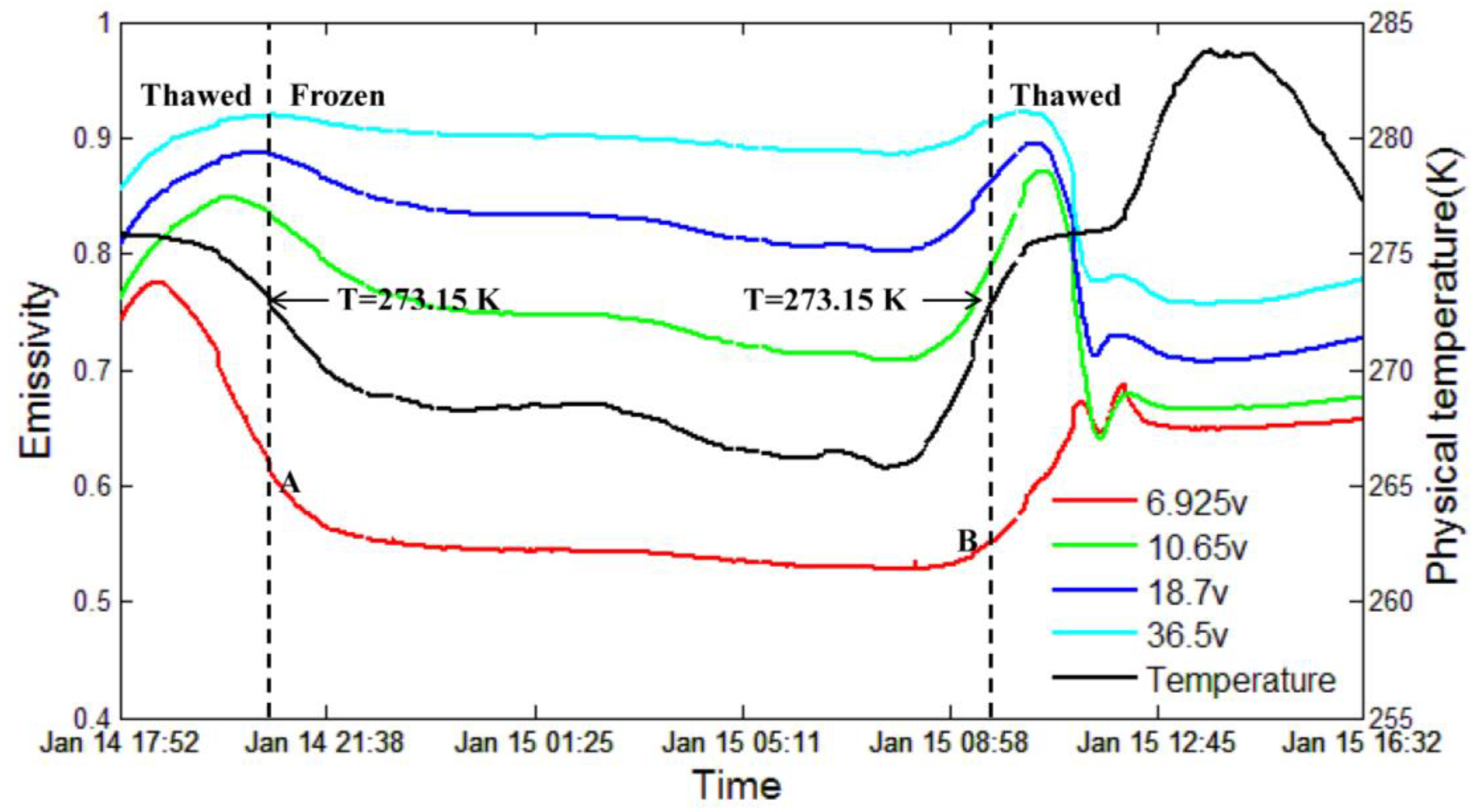
Typical brightness temperature and physical temperature variations are shown in Figure 8. (using a 0.63 cm-thick sample as an example). It can be seen that the soil on the aluminum sheet experienced a thaw-freeze-thaw cycle from 17:52 on 14 January to 16:32 on 15 January. The lowest physical temperature was 265.7K (−7.45 °C), which occurred at 7:47. The highest temperature was 283.7 K (10.55 °C), which occurred at 13:41.
In the experiment, the aluminum sheets were the “cold” source. At the beginning of the measurements, all or part of the signal from the aluminum sheet and wet soil was measured by the radiometer. As the soil’s physical temperature decreases, the liquid water in the soil freezes, which weakens the attenuation ability of the soil and increases its emissivity. Thus, the “cold” signal from the aluminum sheet can easily be observed by the radiometer and initially contribute to the total emissions. Due to the low emissivity of the aluminum sheet, the observed emissivity quickly decreased as its contribution increased. Moreover, due to the greater penetrability, the lower frequency emissivity values were smaller. Hence, the emissivity at 6.925 GHz decreased first, followed by 10.65, 18.7, and 36.5 GHz. After the wet soil was completely frozen, the emissivity values became relatively stable at all four frequencies.
During the soil-thawing process, some of the ice melted, forming liquid water, when the temperature increased on the morning of 15 January. Thus, the “cold” signal of aluminum sheet is shielded by the wet soil, and the observed emissivity increases. However, the emissivity decreases as the amount of ice transformed into liquid water increases. As expected, the emissivity again stabilizes when the soil is completely thawed.
The emissivity and physical temperature trends were similar for each soil sample, regardless of thickness. Two emissivity values exist for each frequency at a given physical temperature (e.g., points A and B on the 6.925 GHz vertical polarization line in Figure 8). At point A, the soil temperature is decreasing from 0+ to 0− °C (‘+’ and ‘−’ indicate that the temperature is just above or below 0 °C). Thus, the soil was freezing. In contrast, point B (from 0− to 0+ °C) corresponds to thawing. Although the temperatures are equal, the physical processes are different, resulting in small emissivity differences. According to a previous experimental study [9,26], at the same negative soil temperature, more unfrozen water can be found in frozen soil during freezing than thawing. Therefore, the unfrozen soil in the thawing process lags behind that in the freezing process. Hence, the unfrozen water content at point B is smaller than at point A. Accounting for the “cold” signal of the aluminum sheet, the observed emissivity at point A is larger than at point B.
To further analyze the emissivity difference in the same negative temperature between freezing and thawing process, we analyzed the measured emissivity with temperature of 268 K, 269 K, 270 K, 271 K, and 272 K. The emissivity at different frequencies during freezing and thawing process was shown in Figure 9. It has shown that the emissivity at all frequencies during freezing process were higher than that during thawing process with the same soil sample temperature.
3.2. Theoretical Model Validation
The theoretical model was evaluated based on the field experiment radiometer measurements. Five soil samples of different thicknesses were analyzed. The measured emissivities with the soil temperature of 268 K, 269 K, 270 K, 271 K, and 272 K in the field experiment were selected to compare with the corresponding simulated emissivities. The parameters used in emissivity simulation were listed in Table 3. Figure 10 illustrates the comparison between measured and simulated emissivity values for the four frequencies: 6.925, 10.65, 18.7, and 36.5 GHz, during the freezing and thawing processes. As described above, there is little difference between the freezing and thawing soil processes. The RMSEs between the simulated and observed emissivity values are 0.076 and 0.096 for the freezing and thawing processes, respectively.
3.3. Parameterized Model Validation
Five soil samples of different thicknesses were studied in the experiment. Accounting for the emissivity of the aluminum sheet as the background value (soil thickness = 0), we obtained six points on the curve expressing the relationship between emissivity and soil thickness for a given soil physical temperature. Soil thickness is the only variable that affects the observed emissivity if the physical temperature is fixed. The emissivity will increase with increasing soil thickness due to the low emissivity of the aluminum sheet, eventually reaching a stable value. However, due to the time and material limitations of this experiment, we cannot create enough soil samples with varying thicknesses to reach these stable emissivity levels for the four frequencies analyzed. Thus, the least square method was used to fit the curves using experimental data. Furthermore, considering the relationship between the measured emissivity and soil thickness introduced in the expression for the MRRD, the exponential form was used to fit the curves.
Where, is the fitted emissivity based on experiment measurements, st is soil thickness in cm. , , and is coefficients.
Using a physical temperature of 268 K as an example, Figure 11 shows the measured and fitted emissivity values as a function of soil thickness at 6.925, 10.65, 18.7, and 36.5 GHz. The initial soil moisture is 0.433 cm3/cm3. As the soil thickness increases, the stable values of emissivity at lower frequencies lags behind that at higher frequencies because lower frequencies can penetrate greater soil depths. Moreover, there is little difference between the freezing (soil temperature varying from 268+ to 268− K) and thawing processes (from 268− to 268+ K) of soil, as noted above.
Using the fitted curve obtained to describe the relationship between the emissivity and soil thickness, it is feasible to estimate the MRRD. The MRRD can be calculated based on the fitted curve for each frequency at a given physical temperature.
The parameterized model was evaluated based on the radiometer measurements from the field experiment. The emissivity values were selected based on a single physical temperature, thereby guaranteeing a consistent soil condition at different soil thicknesses. Thus, the soil thickness is the only variable affecting the observed emissivity for a given frequency. The soil physical temperatures used in this study are 268 K, 269 K, 270 K, 271 K, and 272 K. The MRRD was calculated based on the previously discussed methods at each physical temperature and all four TRMM frequencies (6.925, 10.65, 18.7 and 36.5 GHz). The MRRD can also be estimated using the parameterized model. Because the MRRD from the model and experiment were derived with different incident angles, they must be modified to the appropriate depth at 90° using the real angle of transmission [13]. The estimated MRRD is plotted with the measured values in Figure 12. A good agreement can be seen between the two parameters, except for several points at a low frequency (6.925 GHz), which display a higher MRRD. Our previous study [27] focused on the coherent effects of freezing soil, which may be significant in ground radiometric experiments, especially when using a low-frequency radiometer. This effect could be attributed to the interference caused by frozen layer thickness variations, which results in brightness temperature oscillations (Figure 11). However, the theoretical model used in this study is a non-coherent model, which does not include interference. Furthermore, due to the time limitation and avoiding a heterogeneous frozen soil sample in this experiment, the thickest soil sample was only 1.06 cm. It limited the accuracy of the fitted curves, especially the measurements at lower frequencies, i.e. 6.925 GHz. The fitting curve introduced errors to results of measured MRRD at 6.925 GHz and resulted in disagreement of measured and estimated MRRDs. Therefore, the estimated points at 6.925 GHz do not agree well with the measured MRRD.
The averaged root mean square errors (RMSE) of the soil at the four frequencies are 0.402 cm and 0.537 cm for the thawing and freezing processes, respectively. Note that the validation conducted based on controlled experimental data (i.e., specific soil moistures, textures, temperatures and other parameters). In addition, the parameterized model accuracy is difficult to address based on real soil data. However, the parameterized model was derived based on the radiative transfer theory and the assumptions are both reasonable and consistent with previous research. Thus, there is reason to believe that the developed parameterized model offers an acceptable and simple way for estimating the MRRD using three common parameters: temperature, frequency, and specific surface area.
4. Discussion
In this study, the theoretical model was used to describe the soil microwave radiation in the soil freezing and thawing process. It was then used to develop the parameterized model for estimating the MRRD by using multiple regression analysis based on a simulation database. However, the developed parameterized model has its limitations because the diffuse scattering is not taken into consideration. At low microwave frequencies, the wavelength in soil is in the order of several centimeters, which is significantly larger than the soil particles. At high frequencies, which correspond to shorter wavelengths, the soil particles and voids between particles may cause scattering. For the frozen soil, their emission characteristics are similar to very dry soil, due to an absence of liquid water. Thus, scattering is possible, especially at higher frequencies.
However, there are few published models to describe the complicated diffuse scattering of soil. Herein, the diffuse scattering of soil was ignored in our work and the effect of soil diffuse scattering on MRRD estimation was evaluated by analyzing MRRD at different frequencies as a function of the single scattering albedo (Figure 13). It has shown that the single scattering albedo varying from 0.01 to 0.09 resulted in about 0.43, 0.46, 0.56, and 0.75 cm variation of MRRD at 6.925 GHz, 10.65 GHz, 18.7 GHz, and 36.5 GHz, respectively. This finding suggests that the omission of diffused albedo can lead to a slight MRRD overestimation.
The assumption of equal soil moisture and soil temperature throughout the soil is not strictly true. Temperature and moisture gradients exist within the frozen soil, especially when the soil depth is very thick and the soil temperature is approximately 0 °C. Because the soil sample on the aluminum sheet is not very thick and the data used in this study were below −1 °C, the assumption of uniform soil properties with depth is reasonable.
Another explanation for the disagreement between the measured and estimated MRRDs is the difference of aluminium sheet emissivity used in the theoretical model and measurements. Theoretically, aluminium is an ideal conductor and the waves transmitted to a smooth aluminium sheet will be totally reflected [34]. Therefore, the emissivity of the aluminium sheets should be zero at any observation angle or frequency. In the theoretical model, the emissivity of aluminium were set to be zero. Obviously, they are about 0.01 ~ 0.03, which may be caused by the surface oxidation of the aluminium sheets in the experiment (as shown in Figure 11, when the soil thickness is zero, the measured emissivity is not zero). These results were also found in our other field experiments [35].
5. Conclusions
The objective of this work was to develop a simple, accurate approach for calculating the MRRD of frozen soil. The concept of the MRRD was proposed to describe the source of the primary signal of passive microwave remote sensing and provide a specific expression to define the depth. A controlled truck-mounted experiment was conducted using a three-layer setup. A three-layer theoretical model was then introduced and altered to satisfy the specific experimental design of the study. A database was constructed and sensitivity analysis was conducted based on this theoretical model to study the relationship among the MRRD, soil properties, and frequency. According to the sensitivity analysis, the sensitivity of the MRRD to soil bulk density is much less than that of the three main variables temperature, frequency, and specific surface area for the frozen soil. A parameterized model was then developed for estimating the MRRD of frozen soil using three common and easily acquired parameters: temperature, frequency, and specific surface area. Finally, the parameterized model was validated using experimental data. Some interesting conclusions can be made regarding the MRRD of frozen soil. The soil temperature, frequency, and soil texture are the three main variables affecting the MRRD. The MRRD is negatively correlated with soil temperature, frequency, and specific surface area. Additionally, the MRRD is more sensitive to temperature and frequency than specific surface area. Based on the sensitivity analysis, a parameterized model was developed for estimating the MRRD, and the validation results indicated that the parameterized model has an acceptable accuracy. The RMSEs of MRRD at TMMR’s four frequencies were 0.402 cm and 0.537 cm for the thawing and freezing soil processes, respectively. However, because the validation was performed based on controlled experimental data (i.e., specific soil moistures, textures, temperature variations and other parameters), the parameterized model should be further tested in future studies prior to application. This testing could include field data collection and brightness temperature simulation using a radiative transfer model.
Author Contributions
L.J. conceived and designed the study; T.Z. analyzed the data and wrote the paper; S.Z. and Y.P. collected the experiment data; and L.C. and Y.L. contributed analytical tools and methods.
Funding
This work was funded by the National Natural Science Foundation of China under Grant 41801287, 41671334, and 41871228.
Acknowledgments
The authors would like to thank the anonymous reviewers for their valuable comments.
Conflicts of Interest
The authors declare no conflict of interest.
References
- Kurganova, I.; Teepe, R.; Loftfield, N. Influence of freeze-thaw events on carbon dioxide emission from soils at different moisture and land use. Carbon Balance Manag. 2007, 2, 2. [Google Scholar] [CrossRef] [PubMed]
- Yang, Z.; Ou, Y.H.; Xu, X.; Zhao, L.; Song, M.; Zhou, C. Effects of permafrost degradation on ecosystems. Acta Ecologica Sinica 2010, 30, 33–39. [Google Scholar] [CrossRef]
- Yang, J.; Zhou, W.; Liu, J.; Hu, X. Dynamics of greenhouse gas formation in relation to freeze/thaw soil depth in a flooded peat marsh of Northeast China. Soil Biol. Biochem. 2014, 75, 202–210. [Google Scholar] [CrossRef]
- Zuerndorfer, B.; England, A.W. Radiobrightness decision criteria for freeze/thaw boundaries. IEEE Trans. Geosci. Remote Sens. 1992, 30, 89–102. [Google Scholar] [CrossRef]
- Judge, J.; Galantowicz, J.F.; England, A.W.; Dahl, P. Freeze/thaw classification for prairie soils using SSM/I radiobrightnesses. IEEE Trans. Geosci. Remote Sens. 1997, 35, 827–832. [Google Scholar] [CrossRef]
- Zhang, T.; Armstrong, R.L.; Smith, J. Investigation of the near-surface soil freeze-thaw cycle in the contiguous United States: Algorithm development and validation. J. Geophys. Res.-Atmos. 2003, 108, 8860. [Google Scholar] [CrossRef]
- Zhao, T.; Zhang, L.; Jiang, L.; Zhao, S.; Chai, L.; Jin, R. A new soil freeze/thaw discriminant algorithm using AMSR-E passive microwave imagery. Hydrol. Process. 2011, 25, 1704–1716. [Google Scholar] [CrossRef]
- Du, J.; Kimball, J.S.; Azarderakhsh, M.; Dunbar, R.S.; Moghaddam, M.; McDonald, K.C. Classification of Alaska Spring Thaw Characteristics Using Satellite L-Band Radar Remote Sensing. IEEE Trans. Geosci. Remote Sens. 2015, 53, 542–556. [Google Scholar]
- Zhang, L.; Zhao, T.; Jiang, L.; Zhao, S. Estimate of Phase Transition Water Content in Freeze-Thaw Process Using Microwave Radiometer. IEEE Trans. Geosci. Remote Sens. 2010, 48, 4248–4255. [Google Scholar] [CrossRef]
- Schwank, M.; Stahli, M.; Wydler, H.; Leuenberger, J.; Matzler, C.; Fluhler, H. Microwave L-band emission of freezing soil. IEEE Trans. Geosci. Remote Sens. 2004, 42, 1252–1261. [Google Scholar] [CrossRef]
- Wigneron, J.; Chanzy, A.; de Rosnay, P.; Rudiger, C.; Calvet, J. Estimating the Effective Soil Temperature at L-Band as a Function of Soil Properties. IEEE Trans. Geosci. Remote Sens. 2008, 46, 797–807. [Google Scholar] [CrossRef]
- Escorihuela, M.J.; Chanzy, A.; Wigneron, J.P.; Kerr, Y.H. Effective soil moisture sampling depth of L-band radiometry: A case study. Remote Sens. Environ. 2010, 114, 995–1001. [Google Scholar] [CrossRef] [Green Version]
- Ulaby, F.T.; Moore, R.K.; Fung, A.K. Microwave Remote Sensing: Active and Passive. Volume 1—Microwave Remote Sensing Fundamentals and Radiometry; Remote Sensing A; Addison-Wesley Publishing Company: Boston, MA, USA, 1981; Volume 1, ISBN 0-201-10759-7. [Google Scholar]
- Zhou, F.; Song, X.; Leng, P.; Li, Z. An Effective Emission Depth Model for Passive Microwave Remote Sensing. IEEE J. Sel. Top. Appl. Earth Observ. Remote Sens. 2016, 9, 1752–1760. [Google Scholar] [CrossRef]
- Wilheit, T.T. Radiative Transfer in a Plane Stratified Dielectric. IEEE Trans. Geosci. Remote Sens. 1978, 16, 138–143. [Google Scholar] [CrossRef]
- Wang, J.R. Microwave emission from smooth bare fields and soil moisture sampling depth. IEEE Trans. Geosci. Remote Sens. 1987, 25, 616–622. [Google Scholar] [CrossRef]
- Blinn, J.C.; Conel, J.E.; Quade, J.G. Microwave emission from geological materials: Observations of interference effects. J. Geophys. Res. 1972, 77, 4366–4378. [Google Scholar] [CrossRef]
- Paloscia, S.; Pampaloni, P.; Chiarantini, L.; Coppo, P.; Gagliani, S.; Luzi, G. Multifrequency passive microwve remote sensing of soil moisture and roughness. Int. J. Remote Sens. 1993, 14, 467–483. [Google Scholar] [CrossRef]
- Newton, R.W.; Black, Q.R.; Makanvand, S.; Blanchard, A.J.; Jean, B.R. Soil Moisture Information and Thermal Microwave Emission. IEEE Trans. Geosci. Remote Sens. 1982, 20, 275–281. [Google Scholar] [CrossRef]
- Owe, M.; Van de Griend, A.A. Comparison of soil moisture penetration depths for several bare soils at two microwave frequencies and implications for remote sensing. Water Resour. Res. 1998, 34, 2319–2327. [Google Scholar] [CrossRef]
- Laymon, C.A.; Crosson, W.L.; Jackson, T.J.; Manu, A.; Tsegaye, T.D. Ground-based passive microwave remote sensing observations of soil moisture at S-band and L-band with insight into measurement accuracy. IEEE Trans. Geosci. Remote Sens. 2001, 39, 1844–1858. [Google Scholar] [CrossRef]
- Pampaloni, P.; Paloscia, S.; Chiarantini, L.; Coppo, P.; Gagliani, S.; Luzi, G. Sampling depth of soil moisture content by radiometric measurement at 21 cm wavelength: Some experimental results. Int. J. Remote Sens. 1990, 11, 1085–1092. [Google Scholar] [CrossRef]
- Jackson, T.J.; Bindlish, R.; Cosh, M.H.; Zhao, T.; Starks, P.J.; Bosch, D.D.; Seyfried, M.; Moran, M.S.; Goodrich, D.C.; Kerr, Y.H.; et al. Validation of Soil Moisture and Ocean Salinity (SMOS) Soil Moisture Over Watershed Networks in the U.S. IEEE Trans. Geosci. Remote Sens. 2012, 50, 1530–1543. [Google Scholar] [CrossRef]
- Al Bitar, A.; Leroux, D.; Kerr, Y.H.; Merlin, O.; Richaume, P.; Sahoo, A.; Wood, E.F. Evaluation of SMOS Soil Moisture Products Over Continental US Using the SCAN/SNOTEL Network. IEEE Trans. Geosci. Remote Sens. 2012, 50, 1572–1586. [Google Scholar] [CrossRef]
- Dall’Amico, J.T.; Schlenz, F.; Loew, A.; Mauser, W. First Results of SMOS Soil Moisture Validation in the Upper Danube Catchment. IEEE Trans. Geosci. Remote Sens. 2012, 50, 1507–1516. [Google Scholar] [CrossRef]
- Zhang, L.; Shi, J.; Zhang, Z.J.; Zhao, K.G. The Estimation of Dielectric Constant of Frozen Soil-Water Mixture at Microwave Bands. In Proceedings of the 2003 IEEE International Geoscience and Remote Sensing Symposium (IGARSS 2003), Toulouse, France, 21–25 July 2003; Volume 4, pp. 2903–2905. [Google Scholar]
- Zhao, S.; Zhang, L.; Zhang, Y.; Jiang, L. Microwave emission of soil freezing and thawing observed by a truck-mounted microwave radiometer. Int. J. Remote Sens. 2012, 33, 860–871. [Google Scholar] [CrossRef]
- Zheng, D.; Wang, X.; Rogier, V.; Zeng, Y.; Wen, J.; Wang, Z.; Mike, S.; Paolo, F.; Su, B. L-Band Microwave Emission of Soil Freeze-Thaw Process in the Third Pole Environment. IEEE Trans. Geosci. Remote Sens. 2017, 9, 5324–5338. [Google Scholar] [CrossRef]
- Zhao, S.; Zhang, L.; Zhang, Z. Design and Test of a New Truck-Mounted Microwave Radiometer for Remote Sensing Research. In Proceedings of the 2008 IEEE International Geoscience and Remote Sensing Symposium (IGARSS 2008), Boston, MA, USA, 7–11 July 2008; Volume 2, pp. 1192–1195. [Google Scholar]
- Dobson, M.C.; Ulaby, F.T.; Hallikainen, M.T.; El-rayes, M.A. Microwave Dielectric Behavior of Wet Soil-Part II: Dielectric Mixing Models. IEEE Trans. Geosci. Remote Sens. 1985, GE-23, 35–46. [Google Scholar] [CrossRef]
- Anderson, D.M.; Tice, A.R. Predicting unfrozen water contents in frozen soils from surface area measurements. Highw. Res. Rec. 1972, 12–18. [Google Scholar]
- Ersahin, S.; Gunal, H.; Kutlu, T.; Yetgin, B.; Coban, S. Estimating specific surface area and cation exchange capacity in soils using fractal dimension of particle-size distribution. GEODERMA 2006, 136, 588–597. [Google Scholar] [CrossRef]
- Nedeltchev, N.M. Thermal microwave emission depth and soil moisture remote sensing. Int. J. Remote Sens. 1999, 20, 2183–2194. [Google Scholar] [CrossRef]
- Guru, B.S.; Hiziroglu, H.R. Electromagnetic Field Theory Fundamentals; Cambridge University Press: Cambridge, UK, 2004; ISBN 0-521-83016-8. [Google Scholar]
- Chai, L.; Zhang, L.; Shi, J.C.; Wu, F. Equivalent scattering albedo estimation of cotton and soybean. J. Remote Sens. 2013, 17, 17–33. [Google Scholar]
Figure 1.
Viewing scene of the truck-mounted multi-frequency microwave radiometer (TMMR).

Figure 2.
The flow chart of the parameterized model development and validation process.

Figure 3.
The emissions from layer 2 and layer 3 into layer 1 (air).

Figure 4.
The microwave radiation response depth (MRRD) computed using the theoretical model as a function of normalized soil temperature (a), soil specific surface area (b), unfrozen soil water content (c), frequency (d), and bulk density (e).
Figure 4.
The microwave radiation response depth (MRRD) computed using the theoretical model as a function of normalized soil temperature (a), soil specific surface area (b), unfrozen soil water content (c), frequency (d), and bulk density (e).

Figure 5.
The fitted result of the relationship between MRRD and soil temperature.

Figure 6.
The fitted results of the relationship between coefficients A(a) and B(b) and frequency.

Figure 7.
The fitted results of the relationship between coefficients a1(a), a2(b), a3(c), b1(d), and b2(e) and specific surface area.
Figure 7.
The fitted results of the relationship between coefficients a1(a), a2(b), a3(c), b1(d), and b2(e) and specific surface area.


Figure 8.
Emissivity and physical temperature variations measured in 0.63 cm-thick soil.

Figure 9.
The measured emissivity at different frequencies during freezing and thawing process.

Figure 10.
Comparison between measured and simulated emissivity using theoretical model during freezing and thawing processes.
Figure 10.
Comparison between measured and simulated emissivity using theoretical model during freezing and thawing processes.

Figure 11.
Measured and fitted relationships between soil thickness and emissivity at four frequencies during the thawing process (a) and freezing process (b).
Figure 11.
Measured and fitted relationships between soil thickness and emissivity at four frequencies during the thawing process (a) and freezing process (b).

Figure 12.
Comparison of measured and estimated MRRDs using the parameterized model.

Figure 13.
MRRD as a function of single scattering albedo at different frequencies.


Table 1.
Setup of the key parameters in the simulation database.
| Parameters | Value |
|---|---|
| Temperature | 243.15 to 271.15 K(−30 to −2 °C) |
| Frequency | 4 to 40 GHz |
| Soil specific surface area | 37.442 to 253.042 m2/g |
| Unfrozen water content | 0.02 to 0.31 cm3/cm3 |
| Bulk density | 1.2 to 1.8 g/cm3 |
| Incident angle | 55° |
| Initial soil moisture | 0.433 cm3/cm3 |
Table 2.
The observed lowest and highest temperature of five soil samples.
| Samples Thickness(cm) | Observation Duration | The Lowest and Highest Temperature(K) |
|---|---|---|
| 0.18 | Jan.12th 21:45~Jan. 13th, 15:24 | 260.3 ~ 294.1 |
| 0.43 | Jan.13th 18:06~Jan. 14th, 16:10 | 263.3 ~ 288.7 |
| 0.63 | Jan.14th 17:52~Jan. 15th, 16:32 | 265.7 ~ 283.7 |
| 0.96 | Jan.15th 17:40~Jan. 16th, 15:56 | 267.5 ~ 275.9 |
| 1.06 | Jan.17th 17:30~Jan. 19th, 09:53 | 268.5 ~ 277.8 |
Table 3.
Setup of the key parameters in emissivity simulation.
| Parameters | Value |
|---|---|
| Temperature | 268 K, 269 K, 270 K, 271 K, and 272 K |
| Frequency | 6.925, 10.65, 18.7, and 36.5 GHz |
| Soil texture | sand: 30.16%, silt: 48.85%, clay: 20.99% |
| Bulk density | 1.41 g/cm3 |
| Initial soil moisture | 0.433 cm3/cm3 |
© 2019 by the authors. Licensee MDPI, Basel, Switzerland. This article is an open access article distributed under the terms and conditions of the Creative Commons Attribution (CC BY) license (http://creativecommons.org/licenses/by/4.0/).
Share and Cite
MDPI and ACS Style
Zhang, T.; Jiang, L.; Zhao, S.; Chai, L.; Li, Y.; Pan, Y. Development of a Parameterized Model to Estimate Microwave Radiation Response Depth of Frozen Soil. Remote Sens. 2019, 11, 2028. https://doi.org/10.3390/rs11172028
AMA Style
Zhang T, Jiang L, Zhao S, Chai L, Li Y, Pan Y. Development of a Parameterized Model to Estimate Microwave Radiation Response Depth of Frozen Soil. Remote Sensing. 2019; 11(17):2028. https://doi.org/10.3390/rs11172028
Chicago/Turabian StyleZhang, Tao, Lingmei Jiang, Shaojie Zhao, Linna Chai, Yunqing Li, and Yuhao Pan. 2019. "Development of a Parameterized Model to Estimate Microwave Radiation Response Depth of Frozen Soil" Remote Sensing 11, no. 17: 2028. https://doi.org/10.3390/rs11172028
Note that from the first issue of 2016, this journal uses article numbers instead of page numbers. See further details here.