Remote Sensing Estimation of Lake Total Phosphorus Concentration Based on MODIS: A Case Study of Lake Hongze


1
Key Laboratory of Watershed Geographic Sciences, Nanjing Institute of Geography and Limnology, Chinese Academy of Sciences, Nanjing 210008, China
2
University of Chinese Academy of Sciences, Beijing 100049, China
*
Author to whom correspondence should be addressed.
Remote Sens. 2019, 11(17), 2068; https://doi.org/10.3390/rs11172068
Submission received: 12 August 2019
/
Revised: 31 August 2019
/
Accepted: 1 September 2019
/
Published: 3 September 2019
(This article belongs to the Special Issue Satellite Monitoring of Water Quality and Water Environment)
Abstract
:Phosphorus (P) is an important substance for the growth of phytoplankton and an efficient index to assess the water quality. However, estimation of the TP concentration in waters by remote sensing must be associated with optical substances such as the chlorophyll-a (Chla) and the suspended particulate matter (SPM). Based on the good correlation between the suspended inorganic matter (SPIM) and P in Lake Hongze, we used the direct and indirect derivation methods to develop algorithms for the total phosphorus (TP) estimation with the MODIS/Aqua data. Results demonstrate that the direct derivation algorithm based on 645 nm and 1240 nm of the MODIS/Aqua performs a satisfied accuracy (R2 = 0.75, RMSE = 0.029mg/L, MRE = 39% for the training dataset, R2 = 0.68, RMSE = 0.033mg/L, MRE = 47% for the validate dataset), which is better than that of the indirect derivation algorithm. The 645 nm and 1240 nm of MODIS are the main characteristic band of the SPM, so that algorithm can effectively reflect the P variations in Lake Hongze. Additionally, the ratio of the TP to the SPM is positively correlated with the accuracy of the algorithm as well. The proportion of the SPIM in the SPM has a complex effect on the accuracy of the algorithm. When the SPIM accounts for 78%, the algorithm achieves the highest accuracy. Furthermore, the performance of this direct derivation algorithm was examined in two inland lakes in China (Lake Nanyi and Lake Chaohu), it derived the expected P distribution in Lake Nanyi whereas the algorithm failed in Lake Chaohu. Different water properties influence significantly the accuracy of this direct derivation algorithm, while the TP, Chla, and suspended particular inorganic matter (SPOM) of Lake Chaohu are much higher than those of the other two lakes, thus it is difficult to estimate the TP concentration by a simple band combination in Lake Chaohu. Although the algorithm depends on the dataset used in the development, it usually presents a good estimation for those waters where the SPIM dominated, especially when the SPIM accounts for 60% to 80% of the SPM. This research proposed a direct derivation algorithm for the TP estimation for the turbid lake and will provide a theoretical and practical reference for extending the optical remote sensing application and the TP empirical algorithm of Lake Hongze’s help for the local government management water quality.
1. Introduction
In recent years, with the rapid development of the economy, the intensity of land development and human activities is increasing, P emissions from point sources and non-point sources are increasing year by year in China. Lake pollution has been aggravating in the eastern plain lake zone of China [1,2,3]. In addition to some lakes that have been seriously polluted, some lakes are undergoing eutrophication, for instance, the water quality of Lake Hongze, the fourth largest freshwater lake in China, decreased drastically [4], with the lake becoming turbid and the water more eutrophic [5,6].
Traditional water quality monitoring relies on monitoring stations or lake tour gauging. It is difficult for stations to obtain information on the entire lake, and there is contingency. Moreover, the tour gauging is time-consuming and laborious. Hence, it is critical to be able to estimate the water properties accurately and quickly. For this task, it is believed that remote sensing technologies are the most convenient way to provide such information.
P is an important indicator of the biological growth and eutrophication of lakes. Monitoring the concentration of the TP is an important activity in water quality management [7,8]. Although the influence of the TP concentration on the observed spectrum and remote sensing monitoring procedures is not yet clear, TP is closely related to many substances that affect the reflection spectra [9,10,11,12]. The TP could affect the growth and reproduction of plankton in the water [13], in addition, TP is associated with optical active constituents (OACs) in the water, including the SPM, Chla and chromogenic dissolved organic matter (CDOM) [12,14,15]. These three substances are the main substances that determine the optical characteristics of the water bodies [16,17,18]. Many studies have found the relationship between the spectral reflectance and TP by statistical methods, but there is no unified conclusion [19,20,21]. For example, Gong et al. [19] found a relationship between P and the reflectance at 350 nm; Isenstein and Park [20] used red and mid-infrared bands to estimate the TP concentration in Lake Champlain; Kutser et al. [21] found that 415~455, 655~685, and 405~605 nm can be used to estimate the TP concentration in Lake Peipsi. Not only are there differences in the characteristic bands, but also in the construction method of the estimation algorithms. Presently, all of the TP concentration remote sensing estimation studies are based on empirical methods, which can be divided into two methods. 1) The first method is direct derivation, which uses the statistical linear or non-linear relationship between the reflectance and the in situ P concentration to derive the TP concentration [10,11,12,20,22,23,24]. Although the algorithm deduced often has a high accuracy, the complex debugging process and algorithm structure cannot explain the estimation mechanism clearly. 2) The second method is indirect derivation, which is divided into two steps. First, developing an algorithm for predicting the OAC concentration based on the remote sensing reflectance (Rrs) with a clear theoretical basis. Then, estimating the P concentration by an empirical relationship between the OAC and P concentration [12,25,26]. The indirect derivation method can explain the mechanism of the algorithm, but the algorithm is often difficult to obtain a high precision, because of the propagation and accumulation of uncertainty in the two-step calculation.
In summary, although currently the band used to estimate P is not clear, estimation algorithms are uncertain [19,20,21], the environmental significance of the TP is important, and the TP is closely related to the OACs, hence some studies have attempted to estimate the TP concentration in waters by remote sensing and have been successful. The existing remote sensing estimation algorithms of the TP concentration are derived from empirical methods, which can be divided into direct derivation and indirect derivation. Most of the studies only develop the algorithm, do not use the algorithm in other lakes or different environments, the algorithm performance is not discussed [12,20,23,24,25,27,28].
The goal of this research is to develop an algorithm for the TP estimation in Lake Hongze using MODIS/Aqua. The main objectives are to: (1) Compare the accuracy of the direct derivation algorithm and indirect derivation algorithm, to determine the optimal method and discuss the uncertainty of the optimal algorithm; (2) the rationality and performance evaluation of the optimal algorithm, and the applicability of these two modeling methods in other lakes is discussed.
2. Materials and Methods
2.1. Study Area
Lake Hongze (33°06′–33°40′N, 118°10′–118°52′N) is a shallow lake located in east China. The area covered by Lake Hongze varies with the water levels. When the water level is 12.5 m, the lake’s area is 1597 km2, and its volume is 3.04 billion m3 [5]. The lake’s average water depth is 1.9 m, and its maximum water depth is 4.5 m [29,30]. The inflowing rivers of Lake Hongze are located in the western part of the lake, mainly including the Huai River, Wo River, Wei River, and An River. The main upstream river is the Huai River, which is the most important input source of Lake Hongze, and the water inflow into the lake accounts for more than 70% of the total inflow of all rivers into the lake [5]. The average annual temperature is 16.3 °C. Affected by the monsoon climate, Lake Hongze has an abundant rainfall, with an annual rainfall of 925.5 mm, with the amount of precipitation during June–September accounting for 65.5% of the annual precipitation.
According to the survey of domestic scholars, the water quality of Lake Hongze deteriorated significantly after 2012 [5]. First, the rapid urbanization and industrialization in recent years have resulted in an increase in the point source pollution. Additionally, the land use structure changed, the forest land area is reduced, resulting in aggravation of the non-point source pollution. [31,32]. Then, there are many enclosure culture areas in Lake Hongze, shown as the black mesh in Figure 1, especially in the west lake region, which is surrounded by local fishermen for breeding, feeds, and fertilizers that can lead to an increase in the nutrients [33]. Furthermore, illegal sand mining activities frequently occurred since 2012, resulting in the rapid increase of the SPM concentration in the lake [34]. The resuspension of sediments induced by mining activities has an important effect on the nutrient concentration of the lakes [35,36].
2.2. Field Data and Laboratory Analysis
Four field trips to Lake Hongze were completed on 18 February 2016 (201602), 29 July 2016 (201607), 16 December 2016 (201612) and 25 August 2018 (201808), and 57 samples were collected from 24 stations (Figure 1). An ASD FieldSpec Pro FR (350 nm–1050 nm) was used to measure the spectral reflectance, the measurement process follows the National Aeronautics and Space Administration (NASA) Ocean Optics Protocol [37]. Surface water (depth of 0~50 cm) were collected and stored in the dark and kept cool with ice bags before reaching the laboratory. The sample pretreatment was carried out on the same day. At the same time, the environmental parameters, such as the wind speed, wind direction, and sampling time were recorded.
The samples for TP were acidified with H2SO4 to pH < 1, then the samples were preserved at 2~4 °C. The TP concentrations were determined through a spectrophotometric analysis after the potassium persulfate decomposed [11,38]. The SPM concentrations were gravimetrically determined from the samples collected on pre-combusted and pre-weighed GF/F filters with a diameter of 47 mm that were dried at 105 °C overnight. The filter was weighed on an analytical balance with a precision of 0.01 mg. SPM was differentiated into the SPIM and suspended particular organic matter (SPOM). The SPIM concentration was measured by burning the organic matter from the filters at 450 °C for 4 h and then re-weighing the filters [30,39]. The samples for the Chla were filtered by the GF/F glass fiber membrane and stored in the dark. After repeated freezing and thawing with liquid nitrogen three times, the Chla concentration was measured by the acetone extraction and spectrophotometry [37,40].
2.3. MODIS Data Processing
The MODIS/Aqua Level-1A data for Lake Hongze were downloaded from NASA’s archive (https://oceandata.sci.gsfc.nasa.gov/). First, the Level-1A data were processed using the SeaDAS 7.3 to generate the Level-1B data. Next, the atmospheric correction is needed, which is divided into the Rayleigh scattering correction and aerosol correction. Common methods of the atmospheric correction in the inland water include the Management Unit of the North Sea Mathematical Models (MUMM) and shortwave infrared (SWIR). However, the assumption of dark pixels in the MUMM algorithm is invalid in inland turbid lakes, and the low signal-to-noise ratio in the short-wave band leads to the increase of uncertainty in SWIR. Therefore, these atmospheric correction algorithms are mainly used for ocean remote sensing, so that the correction accuracy of the inland turbid water is insufficient [41,42]. A large number of studies have proved that lake water properties can be estimated successfully by the Rayleigh-corrected reflectance (Rrc, dimensionless) [43], for example, SPM can be estimated by the MODIS Rrc in Lake Hongze [5] and Lake Poyang [44], and Chla can be estimated by the MODIS Rrc in Lake Taihu [45]. Rrc was derived after correction for the Rayleigh scattering and gaseous absorption effects following [43]:
where λ is the wavelength of the MODIS spectral band, is the calibrated at-sensor radiance after correcting for the gaseous absorption, F0 is the extraterrestrial solar irradiance, θ0 is the solar zenith angle, and Rr is the reflectance due to the Rayleigh scattering, which was estimated using the 6S radiative transfer code. The corrected image is resampled to a 250 m resolution and then registered using the Geographic Lookup Table geometric correction. The water quality parameters can be estimated by remote sensing after the Rrc of each band is extracted according to the coordinates of the sampling points.
2.4. Modeling Method and Accuracy Assessment
The direct derivation algorithm was developed according to the following steps: (1) The key OAC of Lake Hongze was determined according to the results of the water properties. In the reference published research, the key OAC characteristic bands were determined; (2) any two characteristic bands were combined according to the addition, subtraction, multiplication, division, and normalization algorithms, and enumerated all the combinations. The correlation coefficients between all the band combinations and TP were calculated. The optimal band combination was selected based on the correlation coefficient; (3) thirty-eight points were randomly selected for modeling, and 19 points were used for verification. The linear, exponential, logarithmic, and power functions were used to fit the TP concentration, and the optimal empirical algorithm was determined.
The indirect derivation algorithm was developed according to the following steps: (1) The key OAC of Lake Hongze was determined according to the results of the water properties; (2) the key OAC concentrations algorithms in Lake Hongze were developed according to the published research, 38 points were randomly selected for modeling, and 19 points were used for verification, the optimal key OAC algorithm is determined; (3) estimating the TP concentration by the empirical relationship between the key OAC and in situ P concentration, 38 points were randomly selected for modeling, and 19 points were used for verification. The linear, exponential, logarithmic, and power functions were used to fit the TP concentration, and the optimal empirical algorithm was determined; (4) step 2 and step 3 were combined to derive the final algorithms, and the algorithms accuracy were evaluated to determine the optimal indirect derivation algorithm.
The determinant coefficient (R2), root mean square error (RMSE), mean relative error (MRE), and Bias were used to evaluate the algorithms accuracy:
3. Results
3.1. Determination of Key OAC
Table 1 shows the results of the sample measurements. The TP concentration of most of the samples is below 0.2 mg/L, indicating that the lake has not reached a serious eutrophication yet. The Chla concentration was low with a mean value of 14.7 μg/L. In addition, the SPM concentration was high in Lake Hongze with an average of 34.8 mg/L, and the mean value in winter was slightly higher than that in summer. In addition, the proportion of the SPIM in the SPM accounts for more than 70% on average in Lake Hongze. Lake Hongze showed a high SPM and low Chla concentration, indicating that the key OAC of Lake Hongze is mainly the SPM.
Since it has been determined that the key OAC of Lake Hongze is the SPM, the band and algorithm are selected directly according to the published research (Table 2). MODIS has been applied in the retrievals of OACs in the case-2 waters in China. Since SPM can reflect a near infrared band, and a lot of studies have successfully estimated the Lake SPM concentration through the near infrared band. The main bands for the SPM retrieval from MODIS are the B1 (645 nm), B2 (859 nm), and B5 (1240 nm), and the estimation algorithms are mainly the linear algorithm and exponential algorithm.
3.2. Development and Validation of Algorithm for TP Estimation
Since the SPM is the main water-color parameter affecting the optical properties, as well as the key OAC affecting the TP. According to Table 2, the B1, B2, and B5 nm bands were selected to build the estimation model of the TP concentration. The enumeration method is used to calculate the correlation coefficients of various band combinations and TP. Table 3 shows all of the single-band correlation coefficients and the three band combinations with the highest correlation coefficient. Most of the single-bands and TP are negatively correlated, with the correlation between the 1240 nm (B5) and TP being the best, with a correlation coefficient of 0.53. Many band combinations show significant correlations with the TP, in particular the (B2−B5)/(B2+B5) and TP have the best correlation, with a value of 0.84.
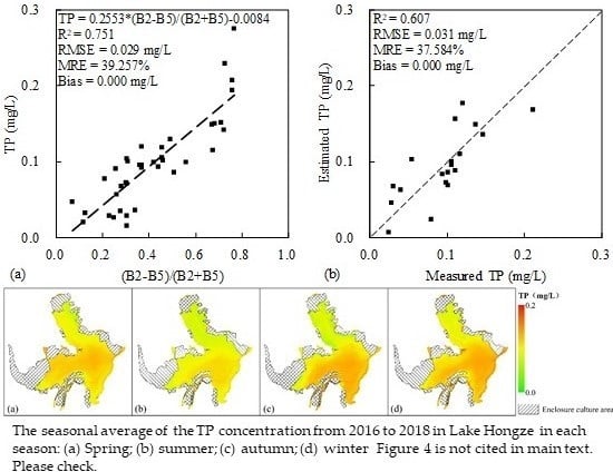
A relatively satisfactory correlation is observed between the field-measured and MODIS- estimated TP concentrations (Figure 2). The optimal algorithm was linear, where the R2 of the training set reached 0.751 (Figure 2a), and the R2 of the verification set reached 0.607 (Figure 2b). The concentrations are uniformly distributed on both sides of the 1:1 line (RMSE = 0.031mg/L, MRE = 37.584%, Bias = 0.000 mg/L), showing that the algorithm has a low error and can estimate the TP over a wide range. The resulting optimal algorithm for the TP estimation in Lake Hongze is given by:
According to Figure 3, a relatively satisfactory correlation is observed between the field-measured and MODIS-estimated SPM concentrations. The optimal algorithm was found to be exponential, where the R2 of the training set reached 0.422 (Figure 3a), and the R2 of the verification set reached 0.605 (Figure 3b). The concentrations are uniformly distributed on both sides of the 1:1 line (RMSE = 15.321mg/L, MRE = 22.574%, Bias = 9.461 mg/L). The optimal algorithm for estimating the TP by the SPM was found to be exponential, where the R2 of the training set was 0.327 (Figure 3c). The estimation equation of the TP was deduced from the first two equations, and it was found to be a linear algorithm (B2–B5), the R2 of the verification set was 0.266 (Figure 3d).
In summary, it can find that: (1) Both the optimal direct derivation algorithm and the optimal indirect derivation algorithm choose the B2 and B5, and the linear algorithm. (2) The accuracy of the direct derivation algorithm was significantly better than that of the indirect derived algorithm.
3.3. Temporal and Spatial Distribution of TP in Lake Hongze
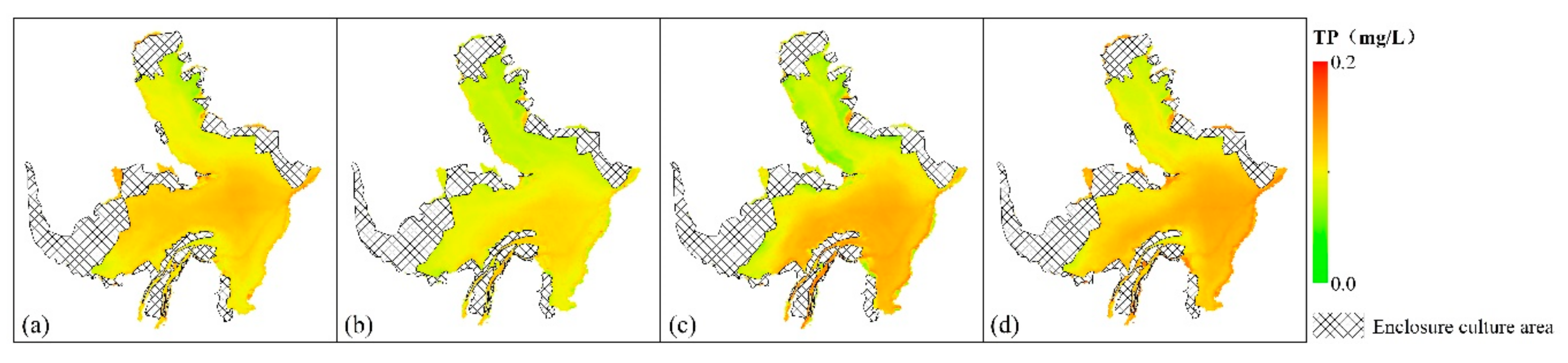
As the algorithms were calibrated with a significantly wide dataset, representing different quality water conditions according to the seasons, the optimal algorithm could be applied in a time-series of the MODIS image. The seasonal average of the TP concentration from 2016 to 2018 is shown in the Figure 4. Due to the complex terrain of the enclosure culture area in Lake Hongze, there was often a field or net to isolate the lake area, but it cannot be recognized on the MODIS image. It was obvious that the TP concentration in the enclosure culture area and lake border is abnormally higher than that in the surrounding area. The TP concentration in Lake Hongze was lower than 0.2 mg/L. Due to the rainfall, the lake water level is high in summer and low in winter, so the TP concentration was the lowest in summer and the highest in winter. The spatial distribution characteristics of the TP concentration in four seasons were basically the same, the TP concentration was the lowest in the northern part of Hongze Lake and the highest in the central part.
4. Discussion
Based on the results from this study, several important points remain. (1) Is there an underlying mechanism that explains why the direct derivation algorithms perform better than the indirect derivation algorithms for Lake Hongze? What are the disadvantages of the indirect derivation algorithms? (2) Why can empirical algorithms estimate the TP? Can this algorithm be interpreted from the perspective of remote sensing? (3) How is the performance of the algorithm? Will other substances influence the algorithm? How to influence? (4) Can the TP algorithm of Lake Hongze be applied to other lakes? Why or why not?
4.1. Why Direct Derivation Algorithms are Better than Indirect Derivation Algorithms in Lake Hongze?
Most studies directly derive the TP estimation algorithm based on reflectance, which shows that the practicability of the direct derivation is better than the indirect derivation, which is consistent with the conclusions drawn in this paper. The reasons for the low accuracy of the indirect derivation include three points: (1) The indirect derivation consists of two steps, first constructing an algorithm for SPM, and then estimating TP by the SPM. In this study, the SPM algorithm is an exponential algorithm, and the SPM and TP relationships are logarithmic. After these two steps, the final algorithm becomes a linear algorithm, which is similar to the algorithm derived directly. Moreover, after two steps, the estimation accuracy will be reduced; (2) the indirect derivation must be based on theoretical knowledge, but the actual situation is often more complicated. TP is not only closely related to the SPM, but also affected by other substances, such as the Secchi depth and Chla [52,53]. In addition, environmental conditions also affect the spatial distribution of the nutrients, e.g., Silio-Calzada et al. [54] found that the spatial temporal variations of nitrate concentrations mimic those of the sea surface temperature. Therefore, estimating the TP based on the OACs alone may not have a good accuracy; (3) in the indirect derivation process, the selection and combination of the bands is fixed, only for the SPM estimation, not necessarily for the TP estimation. The band combination of the direct derivation is more diverse and flexible, and it is possible to construct an algorithm more suitable for estimating the TP.
Therefore, the indirect derivation algorithm is complex and poor in practicability, so it is difficult to establish a reliable indirect derivation algorithm at present. Although the direct derivation algorithm has a high accuracy, it may be contingent and has poor stability. The rationality of the algorithm is explained by a basic theoretical knowledge, and the analysis of the impact on the stability of the algorithm is the next discussion.
4.2. Why the Algorithms can Estimate TP Concentration in Lake Hongze?
The relationship between the TP and SPM is very complicated [55,56,57], with the adsorption capacity of the SPM being different to the TP under various environmental conditions. The TP can be desorbed as a dissolved phosphorus (DP) in the water. However, in most situations, the DP accounts for less than 30% of the TP, leaving more than 70% of the rest in the form of a particulate phosphorus (PP) [2,58,59]. Therefore, the P often has a significant correlation with the SPM [60,61,62]. The correlation coefficients between the TP and different SPM composition were calculated (Table 4). There was a significant positive correlation between the TP and SPM, with a correlation coefficient of 0.53. In particular, the correlation coefficient with the SPIM is the highest, reaching 0.61. Therefore, the key water quality parameters that affect the TP concentration is the SPIM in Lake Hongze. The average concentration of the Chla in Lake Hongze was 14 ug/L, which is much lower than that in other lakes in East China, such as Lake Taihu [17,45] and Lake Chaohu [63], which are basically above 20 ug/L. There was no significant correlation between the Chla and TP, and the low Chla concentration in Lake Hongze indicates that P mainly comes from the sediment, not microorganisms. Next, the correlation coefficient between the band combination and different SPM were calculated. The correlation coefficient between the (B2–B5)/(B2+B5) and SPIM is 0.64, higher than the SPM. The main type of SPM affecting the TP concentration is SPIM, which indicates that the (B2–B5)/(B2+B5) can successfully estimate the TP concentration because of its good correlation with SPIM. Although B2–B5 has the highest correlation coefficient with the SPM, its correlation coefficient with the SPIM is low, which indicates why B2–B5 cannot successfully estimate the TP. Therefore, the SPIM is a key substance for the successful estimation of TP.
In order to clarify the spectral characteristics of the TP and different SPM, the correlation coefficients between these substances and field measured Rrs were calculated (Figure 5), since the noise in the edge region is too large, the 350–400 nm and 900–1050 nm regions were removed [53,62,64]. First, the correlation coefficient of the TP is the lowest, the range of 400–550 nm is decreasing, the range of 550–700 nm is increasing, and then it is slowly decreasing. Sun et al. [11] divided the Lake Taihu water into three types (Type 1, Type 2, Type 3) based on the NTD675 water classification method, and calculated the correlation coefficients of TP and Rrs in the three types of the water bodies, the trend of Type 2 in their study is consistent with the trend of TP in this study, because the water properties of Type 2 is similar to that of Lake Hongze, the Chla/SPM is lower than 0.5 [65], Secondly, the trends of TP, SPM, and SPIM are consistent, but the trends of SPOM are obviously inconsistent, which shows that SPOM spectral characteristics are quite different from the SPIM, and the spectral characteristics of Lake Hongze SPOM have little influence on the spectra of other substances, which is one of the reasons why the reflectance can estimate the TP. Finally, the correlation coefficient is the highest in the B2 region in the four bands, indicating that the band is the best band for estimating the SPM and TP. Duan et al. [53] measured the field Rrs (350−1050 nm) of Lake Nanhu and found that the Rrs of 705–890 nm could reflect the TP concentration. Based on the Rrs of 865 nm, they successfully constructed the TP estimation model, which is similar to the conclusion of this paper.
Due to the low reflectance of the water body, around 10% of the effective information received by the satellite is from the atmosphere, hence the atmospheric correction is an important part of the water color remote sensing [12,66]. It is difficult to obtain highly accurate Rrs values from satellite images of extremely turbid inland waters due to the complex optical conditions, from elevated concentrations of optically active substances to algal blooms [17,67,68]. Since the existing atmospheric correction methods are mainly aimed at relatively clean ocean waters, their applicability is not very appropriate to the study of the inland water quality parameters [5,66,69]. According to the conclusions of other researchers, the required algorithm can be constructed only by the use of Rayleigh-scattering correction results [5,43,44], thus there is a lack of aerosol correction for the time being. However, the two bands ratio and normalization algorithm can reduce the influence of the atmosphere [70,71]. The three band combinations with the highest correlation coefficients listed in Table 3 are all the ratio algorithm and normalization algorithm. The accuracy of estimating the Rrc band normalization is critical to develop the TP algorithm, because the input parameters of this algorithm are the two Rrc band normalization (B2−B5)/(B2+B5).
Although the P is not an optically active substance, there is a significant quantitative relationship between the TP and SPIM in Lake Hongze. SPM is the key water-color parameter of Lake Hongze, the SPIM accounts for 80% of the SPM, and the normalized algorithm can eliminate the atmospheric impact. Therefore, the (B2–B5)/(B2+B5) algorithm can successfully estimate the TP concentration in Lake Hongze, and it is superior to the indirectly derived algorithm.
4.3. How other Substances Affect the Accuracy of the Algorithm?
The concentration and composition of the Chla and SPM will not only affect the optical properties of the lake, but it will also affect the TP concentration [16,17,45]. In order to analyze the influence on the accuracy of the algorithm, the substance concentration and ratio was ranked in an ascending order, each 20 samples were divided into a group, with five samples at the intervals. There are only six groups for the Chla and eight groups for the others. The R2 and RMSE of each group were calculated. The results are shown in Figure 6. Obviously, with the increase of the Chla concentration, the accuracy decreases rapidly, which indicates that when the Chla concentration exceeds 6.81 μg/L, the optical characteristics of the lakes will change (Figure 6a). The characteristic band of the Chla is between 600 nm and 800 nm [64,72,73], so it is impossible to estimate the TP concentration effectively when the Chla concentration increases by (B2−B5)/(B2+B5). It is apparent that with the increasing SPM concentration, the accuracy associated with the algorithm also increases (Figure 6b). When the average concentration of the SPM reached 69 mg/L, the R2 and RMSE reached 0.784 mg/L and 0.037 mg/L, respectively. We speculate that this is due to the enhancement of the spectral reflection signal with the increasing SPM concentration in the water, hence the estimates are more accurate. However, there is a significant positive correlation between the SPM and TP. It is therefore possible that the increasing TP concentrations lead to the improved R2. Therefore, according to the grouping method of the SPM, the accuracy of the algorithm is calculated when the TP/SPM is increased (Figure 6c). It can be seen that with the increase in the TP/SPM, the change in the trend of the RMSE is not obvious, and R2 shows a gradual positive trend. The P is classified into the DP and PP, where the PP accounts for about 70% of the TP [2], microorganisms in the lake water first absorb the biologically active P, which is mainly the DP. This is enhanced when the temperature rises and the microorganisms become more active, leading to the microorganisms absorbing the P more efficiently [74,75,76,77]. Therefore, the increase of the TP/SPM is due to the increase of the P content in the SPM, hence we infer that the increase of the TP content in the SPM, that is, the increase of the PP content, will lead to the increase in the accuracy of the algorithm.
The SPM is also divided into the SPOM and SPIM. The Lake SPIM mainly comes from soil minerals and the SPOM is mainly from microorganisms [78,79]. Although the inorganic P accounts for more than 90% of the TP derived from the soil [77,80]. Microorganisms absorb the bioactive P in the water, mainly the inorganic P, and convert it into nucleotides, which belong to the organic P. Therefore, the composition of the soil P will change rapidly when it enters the lake. When the proportion of the SPIM in the SPM increases, the microbial concentration decreases. Algae particles, which have a strong influence on the inherent optical properties of a water body, are often important factors affecting the estimation of the water color parameters by remote sensing [17], thus the accuracy of the algorithm will increase rapidly. However, when the proportion of the SPIM in the SPM exceeds 78%, the accuracy of the algorithm shows a downward trend (Figure 6d). We speculate that it may be due to the low microbial concentration in the water, such that the DP cannot be absorbed and utilized. The highly-dissolved P concentration, which leads to a poor linear relationship between TP and SPM, will result in an algorithm with a low accuracy. Therefore, when the SPIM accounts for 78% of the SPM, the algorithm has the highest accuracy.
In summary, due to the transformation of TP by microorganisms in the water, the form of the P and the composition of the SPM will also affect the accuracy of the algorithm. The accuracy of the algorithm decreases with the increase of Chla, increases with the increased SPM concentration, as well as with the increased concentration of P in the SPM. The SPIM/SPM has a complex effect on the accuracy of the algorithm, where when the SPIM accounts for 78%, the algorithm achieves the highest accuracy, which then begins to decrease with increasing SPIM.
4.4. Applicability of the Algorithm to other Lakes
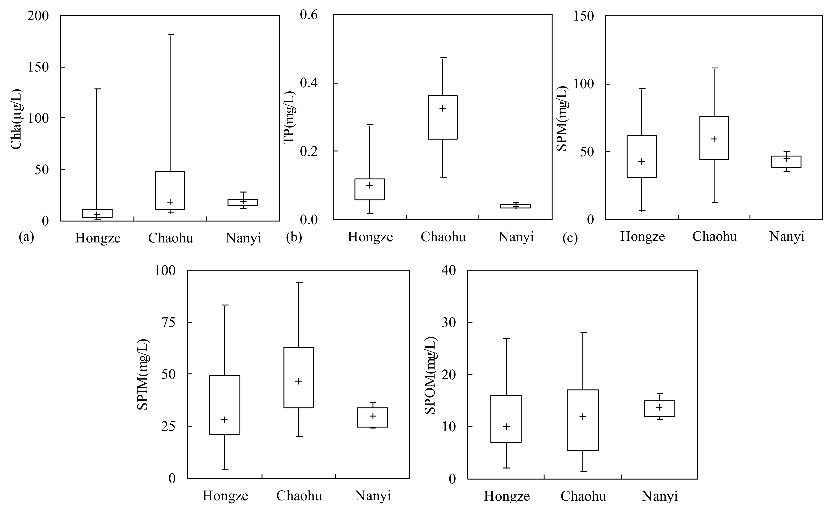
Lake Chaohu and Lake Nanyi are also located in eastern China. Their climatic conditions are similar to those of Lake Hongze and their water bodies are turbid. The upstream rivers of Lake Chaohu are seriously polluted, leading to the water quality of the lake being poor with frequent algal blooms [22]. Lake Chaohu has become one of the most eutrophic lakes in China [13,81]. The water quality of Lake Nanyi is similar to that of Lake Hongze, and eutrophication is not as serious as Lake Chaohu, there are no algae blooms in most time of these years. To examine the applicability of the algorithm in Lake Chaohu and Lake Nanyi, a total of 26 synchronous satellite and ground data points for Lake Chaohu were obtained by following the synchronous satellite and ground data matching criteria. The sampling time is 7 December 2016 and 27 April 2017, respectively. A total of 11 synchronous satellite and ground data points for Lake Nanyi were obtained by following the same criteria. The sampling time is 28 October 2018. The sampling and experimental steps refer to Section 2.2. According to the test results, the water quality differences of the three lakes are shown in Figure 7. Obviously, the eutrophication of Lake Chaohu is the most serious, the TP and Chla concentrations are significantly higher than those of Lake Hongze and Lake Nanyi. The SPIM accounts for 83% of SPM. However, SPIM accounts for 71% and 68% in Lake Hongze and Lake Nanyi, respectively.
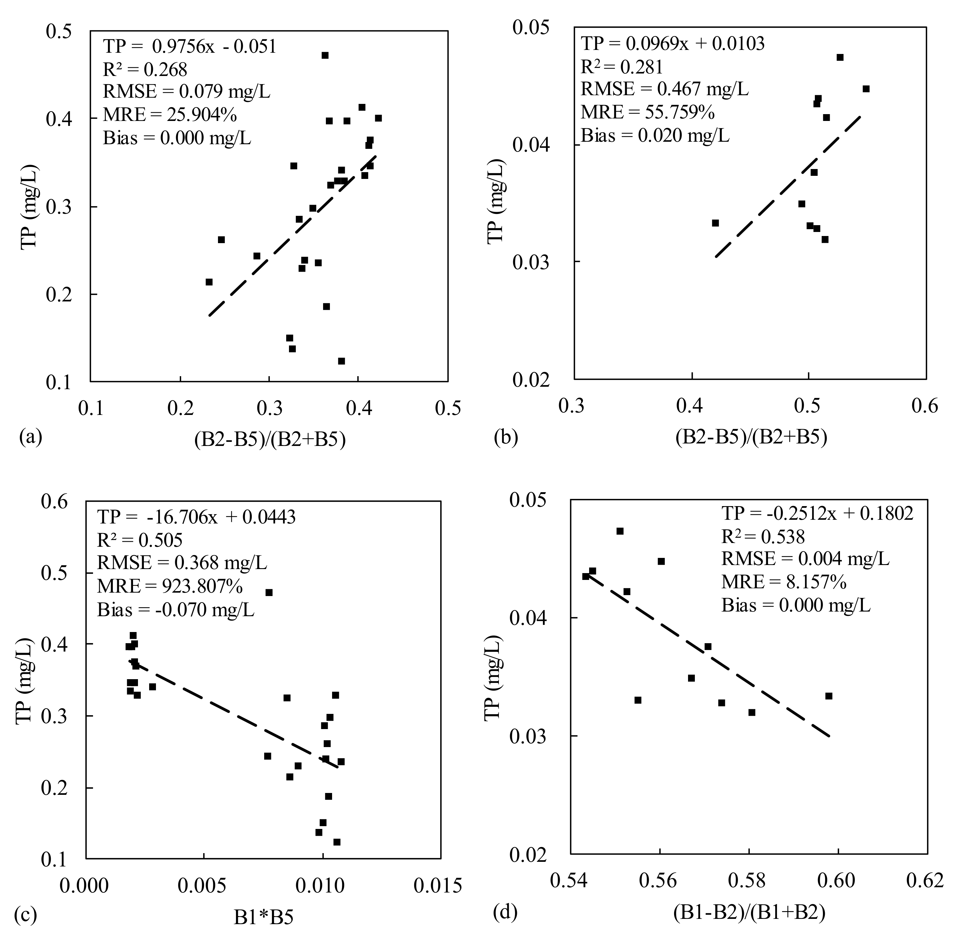
Obviously, the accuracy of the (B2−B5)/(B2+B5) in Chaohu is much lower than that in Lake Hongze (R2 = 0.268, RMSE = 0.079 mg/L, MRE = 25.904%, Bias = 0.000 mg/L). Since the water quality characteristics of Lake Chaohu and Lake Hongze are obviously different. It can be seen from Figure 7 that the TP concentration in Lake Chaohu is significantly higher than the Chla concentration in Lake Hongze, with the concentration of the TP in all sites being above 0.1 mg/L, and the proportion of the SPIM in the SPM is more than 80%, the high proportion of the SPIM will lead to a significant reduction in the accuracy of the algorithm (Figure 6d). The same situation happened in Lake Nanyi, indicating that the (B2−B5)/(B2+B5) is not suitable for the TP estimation of Lake Chaohu and Lake Nanyi (Figure 8). The SPM composition of Lake Nanyi is similar to that of Lake Hongze, and the concentration of the TP is slightly lower than that of Lake Hongze. The average concentration of Chla in Lake Hongze is 18.847 ug/L, and that in Lake Nanyi is 17.73 ug/L. The Chla concentration in the two lakes is similar, however, when the Chla concentration is higher than 6.81 ug/L, the TP algorithm of Lake Hongze will decrease rapidly (Figure 6a), and the lowest chlorophyll concentration of Lake Nanyi will reach 11.243 ug/L. Therefore, the Chla concentration may be considered in estimating the TP concentration of Lake Nanyi.
The TP algorithm of Lake Chaohu and Lake Nanyiare developed by the direct derivation. The results show that although R2 reaches more than 0.5, the points show the bipolar distribution, and the error is large (RMSE = 0.368 mg/L, MRE = 923.807%, Bias = -0.070 mg/L), especially B5 is seriously affected by the atmospheric conditions, so it is difficult to implement the TP algorithm in Lake Chaohu through a simple band combination. At present, there are few studies on the construction of the Chaohu TP estimation algorithm based on the satellite image data, Sun et al. [11] measured the hyperspectral data in the field and divided the water into three categories. They successfully estimated the TP concentrations in several lakes, including Lake Chaohu. As the most eutrophic lake in East China, Lake Taihu is similar to Lake Chaohu. Du et al. [82] used observations from the Global Ocean Color Imager (GOCI) to estimate the TP concentration in Taihu Lake, the algorithm was constructed using the 490, 745, 680 and 865 nm bands. Among them, the 865 nm band is similar to the B5 band employed in this study, with some overlap. The same situation occurred when Chen and Quan [27] estimated the P concentration in Lake Taihu by the use of Landsat images, in which case their algorithm used four bands of the Thematic Mapper (TM). The optical characteristics of Lake Taihu are complicated and are influenced by many substances, since it is extremely eutrophic. When estimating the TP concentration in Lake Taihu, all OACs should be considered comprehensively. However, the optical characteristics of Lake Hongze are mainly dominated by the SPIM, so it is sufficient to use only one band correlated with the SPM. Therefore, in lakes where algal blooms occur frequently, the SPOM will affect the optical properties of the water bodies.
The optimal algorithm was found to be exponential in Lake Nanyi, where the R2 reached 0.538, RMSE is 0.004 mg/L. The TP concentration in Lake Nanyi can be successfully estimated by the direct derivation, but the bands of the Lake Nanyi algorithm and Lake Hongze algorithm are different. A large number of studies have shown that the Chla not only affects the reflectance, but also affects the TP concentration [45], and the characteristic band of the Chla is between 600 nm and 800 nm [64,72,73]. The central wavelength of B1 in the optimal band combination of Lake Nanyi is exactly 645 nm, and the Chla concentration in Lake Nanyi is obviously higher than that in Lake Hongze, which shows that the algorithm takes into account the Chla concentration in Lake Nanyi. Obviously, (B1–B2)/(B1+B2) not only has a good relationship with the Chla, but also has a significant relationship with SPM, especially the SPIM (Figure 9). It proves that if the Lake SPM is dominated by the SPIM, an empirical method can be used to construct an algorithm to estimate the Lake TP concentration. Albert Moses et al. [83] found that there was a significant positive correlation between the ratio of the red band to the infrared band and PO4, and successfully constructed a TP algorithm by the red band, which was consistent with the results in Lake Nanyi. Isenstein and Park [20] successfully estimated the TP concentration of Lake Champlain by the red band and shortwave infrared band, indicating that the red band to the infrared band is the main band for estimating the TP. Therefore, when the Chla concentration exceeds a certain threshold, the TP algorithm must take the Chla into account, but the specific threshold determination needs further study.
By comparing the results of the three lakes, we can find that the two factors influencing the TP estimation are the composition of the SPM and the concentration of Chla. Therefore, there are two conditions for estimating the TP concentration in the lakes by direct derivation: 1) The proportion of SPIM in the SPM ranges from 60% to 80%; 2) the Chla concentration will affect the band and structure of the TP algorithm.
5. Conclusions
In this study, it is proved that the direct derivation is superior to the indirect derivation method in estimating the phosphorus concentration in the lakes. An empirical algorithm based on the MODIS/Aqua data was developed to estimate the TP concentration in Lake Hongze. The algorithm constructs a linear model by the B2 and B5 bands, which is the main characteristic band of SPM. In addition, the normalization algorithm can effectively eliminate the aerosol influence. The accuracy of the resulting algorithm is high, with the R2 of the verification set reaching 0.681, with the RMSE only 0.033 mg/L. Hence, the algorithm could accurately estimate the TP concentrations in Lake Hongze, which is an example of an inland turbid water whose optical characteristics are dominated by the SPM. The TP concentration in Lake Hongze is low in spring and summer and high in autumn and winter. The spatial distribution of the TP in the four seasons is similar. The concentration in the northern region is low and that in the central region is high. Since the algorithm mainly estimates the TP concentration by exploiting the SPM, the applicability of the algorithm under different SPM conditions was analyzed. Due to the transformation of the TP by microorganisms in the water, the form of P and the composition of the SPM will also affect the accuracy of the algorithm. It is found that the accuracy of the algorithm increases with the increasing SPM concentration, as well as when the concentration of P in the SPM increases. However, the SPIM/SPM has a complex effect on the accuracy of the algorithm. When the SPIM accounts for 78%, the algorithm achieves its highest level of accuracy, but then decreases with the increasing SPIM. We also applied the algorithm to Lake Chaohu and Lake Nanyi. It is proved that when the SPIM accounts between 60% and 80% of the SPM, the simple direct derivation can be used to develop a lake TP concentration algorithm. Due to the Chla concentration of Lake Nanyi being significantly higher than that of Lake Hongze, the algorithm of Lake Nanyi includes the B1 band, which is related to the Chla. Based on the algorithms of Lake Hongze and Lake Nanyi, and the results of other researches, the red-to-infrared band has been proved to be the best band for estimating the TP concentration in this kind of lake.
Author Contributions
Data curation, Z.C. and J.X.; investigation, Z.C.; project administration, C.L. and R.M.; supervision, C.L. and R.M.; writing – original draft, J.X.; writing – review & editing, J.X. and Z.C.
Funding
This work was funded by the National Natural Science Foundation of China (41671284, 41771366).
Acknowledgments
Acknowledgement for the data support from “Lake-Watershed Science Data Center, National Earth System Science Data Sharing Infrastructure, National Science & Technology Infrastructure of China. (http://lake.geodata.cn)”.
Conflicts of Interest
The authors declare no conflict of interest.
References
- Ma, R.H.; Duan, H.T.; Hu, C.M.; Feng, X.Z.; Li, A.N.; Ju, W.M.; Jiang, J.H.; Yang, G.S. A half-Century of changes in China’s lakes: Global warming or human influence? Geophys. Res. Lett. 2010, 37. [Google Scholar] [CrossRef]
- Lin, C.; Wu, Z.; Ma, R.; Su, Z. Detection of sensitive soil properties related to non-Point phosphorus pollution by integrated models of SEDD and PLOAD. Ecol. Indic. 2016, 60, 483–494. [Google Scholar] [CrossRef]
- Su, Z.H.; Lin, C.; Ma, R.H.; Luo, J.H.; Liang, Q.O. Effect of land use change on lake water quality in different buffer zones. Appl. Ecol. Environ. Res. 2015, 13, 639–653. [Google Scholar] [CrossRef]
- Ye, C.; Li, C.; Wang, B.; Zhang, J.; Zhang, L. Study on building scheme for a healthy aquatic ecosystem of Lake Hongze. J. Lake Sci. 2011, 23, 725–730. [Google Scholar] [CrossRef]
- Cao, Z.G.; Duan, H.T.; Feng, L.; Ma, R.H.; Xue, K. Climate-and human-Induced changes in suspended particulate matter over Lake Hongze on short and long timescales. Remote Sens. Environ. 2017, 192, 98–113. [Google Scholar] [CrossRef]
- Cao, Z.G.; Duan, H.T.; Shen, M.; Ma, R.H.; Xue, K.; Liu, D.; Xiao, Q.T. Using VIIRS/NPP and MODIS/Aqua data to provide a continuous record of suspended particulate matter in a highly turbid inland lake. Int. J. Appl. Earth Obs. 2018, 64, 256–265. [Google Scholar] [CrossRef]
- Paerl, H.W.; Xu, H.; Hall, N.S.; Rossignol, K.L.; Joyner, A.R.; Zhu, G.W.; Qin, B.Q. Nutrient limitation dynamics examined on a multi-Annual scale in Lake Taihu, China: Implications for controlling eutrophication and harmful algal blooms. J. Freshw. Ecol. 2015, 30, 5–24. [Google Scholar] [CrossRef]
- Paerl, H.W.; Xu, H.; Hall, N.S.; Zhu, G.W.; Qin, B.Q.; Wu, Y.L.; Rossignol, K.L.; Dong, L.H.; McCarthy, M.J.; Joyner, A.R. Controlling Cyanobacterial Blooms in Hypertrophic Lake Taihu, China: Will Nitrogen Reductions Cause Replacement of Non-N-2 Fixing by N-2 Fixing Taxa? PLoS ONE 2014, 9. [Google Scholar] [CrossRef]
- Xiong, J.; Lin, C.; Ma, R.; Wu, Z.; Min, M. Spectral identification of main control factors of soil phosphorus loss from typical agricultural land in Taihu Basin. Bull. Soil Water Conserv. 2017, 37, 137–141. [Google Scholar] [CrossRef]
- Chang, N.B.; Xuan, Z.M.; Yang, Y.J. Exploring spatiotemporal patterns of phosphorus concentrations in a coastal bay with MODIS images and machine learning models. Remote Sens. Environ. 2013, 134, 100–110. [Google Scholar] [CrossRef]
- Sun, D.; Qiu, Z.; Li, Y.; Shi, K.; Gong, S. Detection of total phosphorus concentrations of turbid inland waters using a remote sensing method. Water Air Soil Pollut. 2014, 225, 1–17. [Google Scholar] [CrossRef]
- Wu, C.F.; Wu, J.P.; Qi, J.G.; Zhang, L.S.; Huang, H.Q.; Lou, L.P.; Chen, Y.X. Empirical estimation of total phosphorus concentration in the mainstream of the Qiantang River in China using Landsat TM data. Int. J. Remote Sens. 2010, 31, 2309–2324. [Google Scholar] [CrossRef]
- Yu, L.; Kong, F.X.; Zhang, M.; Yang, Z.; Shi, X.L.; Du, M.Y. The dynamics of microcystis genotypes and microcystin production and associations with environmental factors during blooms in Lake Chaohu, China. Toxins 2014, 6, 3238–3257. [Google Scholar] [CrossRef]
- Li, Y.; Zhang, Y.L.; Shi, K.; Zhu, G.W.; Zhou, Y.Q.; Zhang, Y.B.; Guo, Y.L. Monitoring spatiotemporal variations in nutrients in a large drinking water reservoir and their relationships with hydrological and meteorological conditions based on Landsat 8 imagery. Sci. Total Environ. 2017, 599, 1705–1717. [Google Scholar] [CrossRef]
- Song, K.S.; Li, L.; Wang, Z.M.; Liu, D.W.; Zhang, B.; Xu, J.P.; Du, J.; Li, L.H.; Li, S.; Wang, Y.D. Retrieval of total suspended matter (TSM) and chlorophyll-a (Chl-a) concentration from remote-Sensing data for drinking water resources. Environ. Monit. Assess. 2012, 184, 1449–1470. [Google Scholar] [CrossRef]
- Xue, K.; Zhang, Y.C.; Duan, H.T.; Ma, R.H. Variability of light absorption properties in optically complex inland waters of Lake Chaohu, China. J. Great Lakes Res. 2017, 43, 17–31. [Google Scholar] [CrossRef]
- Shen, M.; Duan, H.T.; Cao, Z.G.; Xue, K.; Loiselle, S.; Yesou, H. Determination of the downwelling diffuse attenuation coefficient of lake water with the Sentinel-3A OLCI. Remote Sens. 2017, 9, 1246. [Google Scholar] [CrossRef]
- Xue, K.; Zhang, Y.C.; Ma, R.H.; Duan, H.T. An approach to correct the effects of phytoplankton vertical nonuniform distribution on remote sensing reflectance of cyanobacterial bloom waters. Limnol. Oceanogr. 2017, 15, 302–319. [Google Scholar] [CrossRef]
- Gong, S.Q.; Huang, J.Z.; Li, Y.M.; Lu, W.N.; Wang, H.J.; Wang, G.X. Preliminary exploring of hyperspectral remote sensing experiment for nitrogen and phosphorus in water. Spectrosc. Spect. Anal. 2008, 28, 839–842. [Google Scholar] [CrossRef]
- Isenstein, E.M.; Park, M.H. Assessment of nutrient distributions in Lake Champlain using satellite remote sensing. J. Environ. Sci. 2014, 26, 1831–1836. [Google Scholar] [CrossRef]
- Kutser, T.; Arst, H.; Miller, T.; Kaarmann, L.; Milius, A. Telespectrometrical estimation of water transparency, chlorophyll-a and total phosphorus concentration of Lake Peipsi. Int. J. Remote Sens. 1995, 16, 3069–3085. [Google Scholar] [CrossRef]
- Li, J.; Zhang, Y.C.; Ma, R.H.; Duan, H.T.; Loiselle, S.; Xue, K.; Liang, Q.C. Satellite-Based estimation of column-integrated algal Biomass in nonalgae bloom conditions: A case study of Lake Chaohu, China. IEEE J. 2017, 10, 450–462. [Google Scholar] [CrossRef]
- Gao, Y.N.; Gao, J.F.; Yin, H.B.; Liu, C.S.; Xia, T.; Wang, J.; Huang, Q. Remote sensing estimation of the total phosphorus concentration in a large lake using band combinations and regional multivariate statistical modeling techniques. J. Environ. Manag. 2015, 151, 33–43. [Google Scholar] [CrossRef]
- El Saadi, A.M.; Yousry, M.M.; Jahin, H.S. Statistical estimation of Rosetta branch water quality using multi-Spectral data. Water Sci. 2014, 28, 18–30. [Google Scholar] [CrossRef]
- Hui, J.; Yao, L. Analysis and inversion of the nutritional status of China’s Poyang Lake using MODIS data. J. Indian Soc. Remote 2016, 44, 837–842. [Google Scholar] [CrossRef]
- Liu, Y.; Jiang, H. Retrieval of total phosphorus concentration in the surface waters of Poyang Lake based on remote sensing and analysis of its spatial-temporal characteristics. J. Nat. Resour. 2013, 28, 2169–2177. [Google Scholar] [CrossRef]
- Chen, J.; Quan, W.T. Using Landsat/TM imagery to estimate nitrogen and phosphorus concentration in Taihu Lake, China. IEEE J. 2012, 5, 273–280. [Google Scholar] [CrossRef]
- He, W.; Chen, S.; Liu, X.; Chen, J. Water quality monitoring in a slightly-Polluted inland water body through remote sensing—Case study of the Guanting Reservoir in Beijing, China. Front. Environ. Sci. Eng. China 2008, 2, 163–171. [Google Scholar] [CrossRef]
- Cai, Y.J.; Lu, Y.J.; Liu, J.S.; Dai, X.L.; Xu, H.; Lu, Y.; Gong, Z.J. Macrozoobenthic community structure in a large shallow lake: Disentangling the effect of eutrophication and wind-Wave disturbance. Limnologica 2016, 59, 1–9. [Google Scholar] [CrossRef]
- Cao, Z.G.; Duan, H.T.; Cui, H.S.; Ma, R.H. Remote estimation of suspended matters concentrations using VIIRS in Lake Hongze, China. J. Infrared Millim. 2016, 35, 462–469. [Google Scholar] [CrossRef]
- Lin, C.; Hu, W.P.; Xu, J.D.; Ma, R.H. Development of a visualization platform oriented to Lake water quality targets management—A case study of Lake Taihu. Ecol. Inform. 2017, 41, 40–53. [Google Scholar] [CrossRef]
- Min, M.; Lin, C.; Xiong, J.F.; Shen, C.Z.; Jin, Z.F.; Ma, R.; Xu, J. Research on spatio-Temporal pattern evolution of NPS particulate phosphorus load in hongze lake basin under different landuse patterns. Resour. Environ. Yangtze Basin 2017, 26, 606–614. [Google Scholar] [CrossRef]
- Zhou, D.; Zhang, Q.; Song, X.; Xie, X. Distribution of heavy metals and potential ecological risk in the surface sediment of Hongze Lake. J. Huaihai Inst. Technol. 2012, 21, 39–43. [Google Scholar] [CrossRef]
- Duan, H.T.; Cao, Z.G.; Shen, M.; Liu, D.; Xiao, Q.T. Detection of illicit sand mining and the associated environmental effects in China’s fourth largest freshwater lake using daytime and nighttime satellite images. Sci. Total Environ. 2019, 647, 606–618. [Google Scholar] [CrossRef]
- Soriano-Disla, J.M.; Speir, T.W.; Gomez, I.; Clucas, L.M.; McLaren, R.G.; Navarro-Pedreno, J. Evaluation of different extraction methods for the assessment of heavy metal bioavailability in various soils. Water Air Soil Pollut. 2010, 213, 471–483. [Google Scholar] [CrossRef]
- Sondergaard, M.; Jeppesen, E.; Lauridsen, T.L.; Skov, C.; Van Nes, E.H.; Roijackers, R.; Lammens, E.; Portielje, R. Lake restoration: Successes, failures and long-Term effects. J. Appl. Ecol. 2007, 44, 1095–1105. [Google Scholar] [CrossRef]
- Ma, R.; Tang, J.; Dai, J. Bio-Optical model with optimal parameter suitable for Taihu Lake in water colour remote sensing. Int. J. Remote Sens. 2006, 27, 4305–4328. [Google Scholar] [CrossRef]
- Xu, H.; Paerl, H.W.; Qin, B.Q.; Zhu, G.W.; Gao, G. Nitrogen and phosphorus inputs control phytoplankton growth in eutrophic Lake Taihu, China. Limnol. Oceanogr. 2010, 55, 420–432. [Google Scholar] [CrossRef]
- Duan, H.T.; Feng, L.; Ma, R.H.; Zhang, Y.C.; Loiselle, S.A. Variability of particulate organic carbon in inland waters observed from MODIS Aqua imagery. Environ. Res. Lett. 2014, 9. [Google Scholar] [CrossRef]
- Wu, J.H.; Duan, H.T.; Zhang, Y.C.; Ma, R.H. A novel algorithm to estimate POC concentrations in Chaohu Lake, China. J. Infrared Millim. 2015, 34, 750–756. [Google Scholar] [CrossRef]
- Hu, C.M.; Feng, L.; Lee, Z.; Davis, C.O.; Mannino, A.; McClain, C.R.; Franz, B.A. Dynamic range and sensitivity requirements of satellite ocean color sensors: Learning from the past. Appl. Opt. 2012, 51, 6045–6062. [Google Scholar] [CrossRef]
- Aurin, D.; Mannino, A.; Franz, B. Spatially resolving ocean color and sediment dispersion in river plumes, coastal systems, and continental shelf waters. Remote Sens. Environ. 2013, 137, 212–225. [Google Scholar] [CrossRef] [Green Version]
- Hu, C.M.; Chen, Z.Q.; Clayton, T.D.; Swarzenski, P.; Brock, J.C.; Muller-Karger, F.E. Assessment of estuarine water-Quality indicators using MODIS medium-Resolution bands: Initial results from Tampa Bay, FL. Remote Sens. Environ. 2004, 93, 423–441. [Google Scholar] [CrossRef]
- Feng, L.; Hu, C.M.; Chen, X.L.; Tian, L.Q.; Chen, L.Q. Human induced turbidity changes in Poyang Lake between 2000 and 2010: Observations from MODIS. J. Geophys. Res. 2012, 117. [Google Scholar] [CrossRef]
- Shi, K.; Zhang, Y.L.; Zhou, Y.Q.; Liu, X.H.; Zhu, G.W.; Qin, B.Q.; Gao, G. Long-Term MODIS observations of cyanobacterial dynamics in Lake Taihu: Responses to nutrient enrichment and meteorological factors. Sci. Rep. 2017, 7. [Google Scholar] [CrossRef]
- Cui, L.J.; Qiu, Y.; Fei, T.; Liu, Y.L.; Wu, G.F. Using remotely sensed suspended sediment concentration variation to improve management of Poyang Lake, China. Lake Reserv. Manag. 2013, 29, 47–60. [Google Scholar] [CrossRef] [Green Version]
- Shi, K.; Zhang, Y.L.; Zhu, G.W.; Liu, X.H.; Zhou, Y.Q.; Xu, H.; Qin, B.Q.; Liu, G.; Li, Y.M. Long-Term remote monitoring of total suspended matter concentration in Lake Taihu using 250 m MODIS-Aqua data. Remote Sens. Environ. 2015, 164, 43–56. [Google Scholar] [CrossRef]
- Wu, G.F.; Liu, L.J.; Chen, F.Y.; Fei, T. Developing MODIS-Based retrieval models of suspended particulate matter concentration in Dongting Lake, China. Int. J. Appl. Earth Obs. 2014, 32, 46–53. [Google Scholar] [CrossRef]
- Jiang, X.W.; Tang, J.W.; Zhang, M.W.; Ma, R.H.; Ding, J. Application of MODIS data in monitoring suspended sediment of Taihu Lake, China. Chin. J. Oceanol. Limnol. 2009, 27, 614–620. [Google Scholar] [CrossRef]
- Wang, J.J.; Lu, X.X. Estimation of suspended sediment concentrations using Terra MODIS: An example from the Lower Yangtze River, China. Sci. Total Environ. 2010, 408, 1131–1138. [Google Scholar] [CrossRef]
- Wang, J.J.; Lu, X.X.; Liew, S.C.; Zhou, Y. Remote sensing of suspended sediment concentrations of large rivers using multi-Temporal MODIS images: An example in the Middle and Lower Yangtze River, China. Int. J. Remote Sens. 2010, 31, 1103–1111. [Google Scholar] [CrossRef]
- Schindler, D. Evolution of phosphorus limitation in lakes. Science 1977, 195, 260–262. [Google Scholar] [CrossRef]
- Duan, H.; Zhang, B.; Song, K.; Huang, S.; Wang, Z.; Zhang, S. Hyperspectral monitoring model of eutrophication in Lake Nanhu, Changchun. J. Lake Sci. 2005, 3, 282–288. [Google Scholar] [CrossRef]
- Silio-Calzada, A.; Bricaud, A.; Uitz, J.; Gentili, B. Estimation of new primary production in the Benguela upwelling area, using ENVISAT satellite data and a model dependent on the phytoplankton community size structure. J. Geophys. Res. 2008, 113. [Google Scholar] [CrossRef]
- Fang, F.; Brezonik, P.L.; Mulla, D.J.; Hatch, L.K. Estimating runoff phosphorus losses from calcareous soils in the Minnesota River Basin. J. Environ. Qual. 2002, 31, 1918–1929. [Google Scholar] [CrossRef]
- Follmi, K.B. The phosphorus cycle, phosphogenesis and marine phosphate-Rich deposits. Earth-Sci. Rev. 1996, 40, 55–124. [Google Scholar] [CrossRef]
- Borggaard, O.K. The influence of iron-Oxides on phosphate adsorption by soil. J. Soil Sci. 1983, 34, 333–341. [Google Scholar] [CrossRef]
- Adhami, E.; Ronaghi, A.; Karimian, N.; Molavi, R. Transformation of phosphorus in highly calcareous soils under field capacity and waterlogged conditions. Soil Res. 2012, 50, 249–255. [Google Scholar] [CrossRef]
- Zhou, A.M.; Tang, H.X.; Wang, D.S. Phosphorus adsorption on natural sediments: Modeling and effects of pH and sediment composition. Water Res. 2005, 39, 1245–1254. [Google Scholar] [CrossRef]
- Shinohara, R.; Imai, A.; Kawasaki, N.; Komatsu, K.; Kohzu, A.; Miura, S.; Sano, T.; Satou, T.; Tomioka, N. Biogenic Phosphorus Compounds in Sediment and Suspended Particles in a Shallow Eutrophic Lake: A P-31-Nuclear Magnetic Resonance (P-31 NMR) Study. Environ. Sci. Technol. 2012, 46, 10572–10578. [Google Scholar] [CrossRef]
- Pan, G.; Krom, M.D.; Zhang, M.Y.; Zhang, X.W.; Wang, L.J.; Dai, L.C.; Sheng, Y.Q.; Mortimer, R.J.G. Impact of suspended inorganic particles on phosphorus cycling in the Yellow River (China). Environ. Sci. Technol. 2013, 47, 9685–9692. [Google Scholar] [CrossRef] [PubMed]
- Song, K.S.; Li, L.; Li, S.; Tedesco, L.; Hall, B.; Li, L.H. Hyperspectral remote sensing of total phosphorus (TP) in three central Indiana water supply reservoirs. Water Air Soil Pollut. 2012, 223, 1481–1502. [Google Scholar] [CrossRef]
- Shang, G.; Shang, J. Spatial and temporal variations of eutrophication in western Chaohu Lake, China. Environ. Monit. Assess. 2007, 130, 99–109. [Google Scholar] [CrossRef]
- Gurlin, D.; Gitelson, A.A.; Moses, W.J. Remote estimation of chl-a concentration in turbid productive waters - Return to a simple two-band NIR-red model? Remote Sens. Environ. 2011, 115, 3479–3490. [Google Scholar] [CrossRef]
- Sun, D.Y.; Li, Y.M.; Wang, Q.; Le, C.F.; Lv, H.; Huang, C.C.; Gong, S.Q. Specific inherent optical quantities of complex turbid inland waters, from the perspective of water classification. Photochem. Photobiol. Sci. 2012, 11, 1299–1312. [Google Scholar] [CrossRef]
- Ma, R.H.; Jiang, G.J.; Duan, H.T.; Bracchini, L.; Loiselle, S. Effective upwelling irradiance depths in turbid waters: A spectral analysis of origins and fate. Opt. Express 2011, 19, 7127–7138. [Google Scholar] [CrossRef]
- Hu, C.M.; Lee, Z.P.; Ma, R.H.; Yu, K.; Li, D.Q.; Shang, S.L. Moderate Resolution Imaging Spectroradiometer (MODIS) observations of cyanobacteria blooms in Taihu Lake, China. J. Geophys. Res. 2010, 115. [Google Scholar] [CrossRef] [Green Version]
- Shi, W.; Wang, M.H. An assessment of the black ocean pixel assumption for MODIS SWIR bands. Remote Sens. Environ. 2009, 113, 1587–1597. [Google Scholar] [CrossRef]
- Kutser, T.; Pierson, D.; Tranvik, L.; Reinart, A.; Sobek, S.; Kallio, K. Using satellite remote sensing to estimate the colored dissolved organic matter absorption coefficient in lakes. Ecosystems 2005, 8, 709–720. [Google Scholar] [CrossRef]
- Stramska, M.; Stramski, D. Variability of particulate organic carbon concentration in the north polar Atlantic based on ocean color observations with Sea-Viewing Wide Field-Of-View Sensor (SeaWiFS). J. Geophys. Res. 2005, 110. [Google Scholar] [CrossRef]
- Liu, G.; Li, Y.M.; Lyu, H.; Wang, S.; Du, C.G.; Huang, C.C. An improved land target-Based atmospheric correction method for Lake Taihu. IEEE J. 2016, 9, 793–803. [Google Scholar] [CrossRef]
- Gitelson, A. The peak near 700 nm on radiance spectra of algae and water: Relationships of Its magnitude and position with chlorophyll concentration. Int. J. Remote Sens. 1992, 13, 3367–3373. [Google Scholar] [CrossRef]
- Gilerson, A.A.; Gitelson, A.A.; Zhou, J.; Gurlin, D.; Moses, W.; Ioannou, I.; Ahmed, S.A. Algorithms for remote estimation of chlorophyll-a in coastal and inland waters using red and near infrared bands. Opt. Express 2010, 18, 24109–24125. [Google Scholar] [CrossRef] [Green Version]
- Sanyal, S.; De Datta, S. Chemistry of phosphorus transformations in soil. In Advances in Soil Science; Springer: New York, NY, USA, 1991. [Google Scholar]
- Scavia, D.; DePinto, J.V.; Bertani, I. A multi-Model approach to evaluating target phosphorus loads for Lake Erie. J. Great Lakes Res. 2016, 42, 1139–1150. [Google Scholar] [CrossRef]
- Liu, Q.; Wan, J.F.; Wang, J.; Li, S.Y.; Dagot, C.; Wang, Y. Recovery of phosphorus via harvesting phosphorus-Accumulating granular sludge in sequencing batch airlift reactor. Bioresour. Technol. 2017, 224, 87–93. [Google Scholar] [CrossRef] [PubMed]
- Zhou, J.; Wu, Y.H.; Jorg, P.; Bing, H.J.; Yu, D.; Sun, S.Q.; Luo, J.; Sun, H.Y. Changes of soil phosphorus speciation along a 120-Year soil chronosequence in the Hailuogou Glacier retreat area (Gongga Mountain, SW China). Geoderma 2013, 195, 251–259. [Google Scholar] [CrossRef]
- Wang, Y.; Liu, R.H.; Zhang, Y.Q.; Cui, X.Q.; Tang, A.K.; Zhang, L.J. Transport of heavy metals in the Huanghe River estuary, China. Environ. Earth Sci. 2016, 75. [Google Scholar] [CrossRef]
- Wu, W.H.; Zheng, H.B.; Xu, S.J.; Yang, J.D.; Liu, W. Trace element geochemistry of riverbed and suspended sediments in the upper Yangtze River. J. Geochem. Explor. 2013, 124, 67–78. [Google Scholar] [CrossRef]
- Sun, G.F.; Jin, J.Y.; Shi, Y.L. Research advance on soil phosphorous forms and their availability to crops in soil. Soil Fertil. Sci. China 2011, 2, 1–9. [Google Scholar] [CrossRef]
- Zhou, Y.L.; Jin, J.L.; Liu, L.; Zhang, L.B.; He, J.; Wang, Z.S. Inference of reference conditions for nutrient concentrations of Chaohu Lake based on model extrapolation. Chin. Geogr. Sci. 2013, 23, 35–48. [Google Scholar] [CrossRef]
- Du, C.; Li, Y.; Wang, Q.; Zhu, L.; Lü, H. Inversion model and daily variation of total phosphorus concentrations in Taihu Lake based on GOCI data. Environ. Sci. 2016, 37, 862–872. [Google Scholar] [CrossRef]
- Albert Moses, S.; Janaki, L.; Joseph, S.; Kizhur Kandathil, R. Determining the spatial variation of phosphorus in a lake system using remote sensing techniques. Lakes Reserv. 2014, 19, 24–36. [Google Scholar] [CrossRef]
Figure 1.
Location of the study site and sampling plots.

Figure 2.
The optimal algorithms obtained by the direct derivation method: (a) The relationship between the in situ measured TP and (B2–B5)/(B2+B5); (b) the validation of the MODIS-estimated TP with the in situ measured TP based on an independent dataset.
Figure 2.
The optimal algorithms obtained by the direct derivation method: (a) The relationship between the in situ measured TP and (B2–B5)/(B2+B5); (b) the validation of the MODIS-estimated TP with the in situ measured TP based on an independent dataset.

Figure 3.
The optimal algorithms obtained by the indirect derivation method: (a) The relationship between the in situ measured SPM and (B2−B5); (b) the validation of the MODIS-estimated SPM with the in situ measured SPM based on an independent dataset; (c) the relationship between the in situ measured TP and MODIS-estimated SPM; (d) the validation of the indirect derivation method-estimated TP with the in situ measured TP based on an independent dataset.

Figure 4.
The seasonal average of the TP concentration from 2016 to 2018 in Lake Hongze in each season: (a) Spring; (b) summer; (c) autumn; (d) winter.
Figure 4.
The seasonal average of the TP concentration from 2016 to 2018 in Lake Hongze in each season: (a) Spring; (b) summer; (c) autumn; (d) winter.

Figure 5.
The correlation coefficients between the SPM, SPIM, SPOM, TP, and Rrs measured in the sites.
Figure 5.
The correlation coefficients between the SPM, SPIM, SPOM, TP, and Rrs measured in the sites.

Figure 6.
Algorithm accuracy change with different substance changes. (a) Chlorophyll-a (Chla); (b) SPM; (c) TP/SPM; (d) SPIM/SPM.
Figure 6.
Algorithm accuracy change with different substance changes. (a) Chlorophyll-a (Chla); (b) SPM; (c) TP/SPM; (d) SPIM/SPM.

Figure 7.
Box-plot of the water quality attributes of the three lakes: (a) Chla; (b) TP; (c) SPM; (d) SPIM; (e) SPOM.
Figure 7.
Box-plot of the water quality attributes of the three lakes: (a) Chla; (b) TP; (c) SPM; (d) SPIM; (e) SPOM.

Figure 8.
(a) Scatter plot of the (B2−B5)/(B2+B5) and TP concentration in Lake Chaohu; (b) scatter plot of the (B2−B5)/(B2+B5) and TP concentration in Lake Nanyi; (c) scatter plot of the B1*B5 and TP concentration in Lake Chaohu; (d) scatter plot of the (B1−B2)/(B1+B2) and TP concentration in Lake Nanyi.

Figure 9.
(a) Scatter plot of the (B1–B2)/(B1+B2) and Chla concentration in Lake Nanyi; (b) scatter plot of the (B1–B2)/(B1+B2) and SPM concentration in Lake Nanyi; (c) scatter plot of the (B1–B2)/(B1+B2) and SPIM concentration in Lake Nanyi; (d) scatter plot of the (B1–B2)/(B1+B2) and SPOM concentration in Lake Nanyi.


Table 1.
Water properties of Lake Hongze.
| Date (Number) | Statistics | TP (mg/L) | SPM (mg/L) | SPIM (mg/L) | SPOM (mg/L) | Chla (μg/L) |
|---|---|---|---|---|---|---|
| 201602 (N = 19) | Range | 0.06~0.13 | 26.00~69.00 | 14.00~58.00 | 2.00~16.00 | * |
| Mean ± SD | 0.10 ± 0.02 | 37.95 ± 17.78 | 30.11 ± 16.31 | 7.84 ±3.27 | * | |
| 201607 (N = 7) | Range | 0.07~0.12 | 25.80~53.80 | 12.47~26.87 | 8.73~26.93 | 6.98~128.37 |
| Mean ± SD | 0.09 ± 0.02 | 36.33 ± 8.36 | 21.43 ± 4.68 | 14.91 ± 6.53 | 47.37 ± 38.73 | |
| 201612 (N = 18) | Range | 0.04~0.28 | 21.00~96.00 | 14.00~83.00 | 3.00~16.00 | 1.38~7.94 |
| Mean ± SD | 0.15 ± 0.06 | 58.47 ± 23.62 | 45.82 ± 21.25 | 12.65 ± 9.34 | 3.46 ± 1.70 | |
| 201808 (N = 13) | Range | 0.02~0.08 | 28.00~69.33 | 9.33~52.00 | 13.33~20.00 | 4.29~33.18 |
| Mean ± SD | 0.03 ± 0.02 | 49.03 ± 14.70 | 32.21 ± 14.74 | 16.82 ± 1.78 | 12.77 ± 9.48 |
Note: SD is the standard deviation. *. Parameters are unmeasured.
Table 2.
Estimation of the suspended particulate matter (SPM) concentration using moderate resolution imaging spectroradiometer (MODIS) in the case-2 waters in China.
Table 2.
Estimation of the suspended particulate matter (SPM) concentration using moderate resolution imaging spectroradiometer (MODIS) in the case-2 waters in China.
| Location | Band | Algorithm | References |
|---|---|---|---|
| Lake Poyang Lake Taihu | Band 1 | SPM=a*exp(b*(B1)) | [46,47] |
| Lake Dongting, Lake Poyang, Lake Hongze | Band 1, Band 5 | SPM=a*exp(b*(B1-B5)) | [5,44,48] |
| Lake Taihu | Band 2 | log10(SPM)=a*ln(B2)+b | [49] |
| Yangtze River | Band 2, Band 5 | SPM=a*exp(b*(B2−B5)) | [50] |
| Yangtze River | Band 2, Band 5 | SPM=a*(B2−B5)+b | [51] |
Table 3.
The correlation coefficient between the total phosphorus (TP) and band/band combination of MODIS.
Table 3.
The correlation coefficient between the total phosphorus (TP) and band/band combination of MODIS.
| Band/Band Combination | B1 | B2 | B5 | (B2−B5)/(B2+B5) | B2/B5 | B1/B5 |
|---|---|---|---|---|---|---|
| Correlation coefficient | 0.23 | 0.33 * | −0.53 ** | 0.84 ** | 0.83 ** | 0.79 ** |
*. Correlation is significant at the 0.05 level (two-tailed). **. Correlation is significant at the 0.01 level (two-tailed).
Table 4.
The correlation coefficient between the water quality index and band combination of MODIS.
| TP | SPM | SPIM | SPOM | Chla | |
|---|---|---|---|---|---|
| TP | 0.53 ** | 0.61 ** | 0.25 | −0.14 | |
| (B2−B5)/(B2+B5) | 0.84 ** | 0.54 ** | 0.64 ** | 0.20 | −0.21 |
| B2−B5 | 0.54 ** | 0.64 ** | 0.53 ** | 0.09 | −0.17 |
**. Correlation is significant at the 0.01 level (two-tailed).
© 2019 by the authors. Licensee MDPI, Basel, Switzerland. This article is an open access article distributed under the terms and conditions of the Creative Commons Attribution (CC BY) license (http://creativecommons.org/licenses/by/4.0/).
Share and Cite
MDPI and ACS Style
Xiong, J.; Lin, C.; Ma, R.; Cao, Z. Remote Sensing Estimation of Lake Total Phosphorus Concentration Based on MODIS: A Case Study of Lake Hongze. Remote Sens. 2019, 11, 2068. https://doi.org/10.3390/rs11172068
AMA Style
Xiong J, Lin C, Ma R, Cao Z. Remote Sensing Estimation of Lake Total Phosphorus Concentration Based on MODIS: A Case Study of Lake Hongze. Remote Sensing. 2019; 11(17):2068. https://doi.org/10.3390/rs11172068
Chicago/Turabian StyleXiong, Junfeng, Chen Lin, Ronghua Ma, and Zhigang Cao. 2019. "Remote Sensing Estimation of Lake Total Phosphorus Concentration Based on MODIS: A Case Study of Lake Hongze" Remote Sensing 11, no. 17: 2068. https://doi.org/10.3390/rs11172068
Note that from the first issue of 2016, this journal uses article numbers instead of page numbers. See further details here.