Classification of Mangrove Species Using Combined WordView-3 and LiDAR Data in Mai Po Nature Reserve, Hong Kong


1
Department of Geography and Resource Management, The Chinese University of Hong Kong, Shatin, New Territories, Hong Kong, China
2
Institute of Future Cities, The Chinese University of Hong Kong, Shatin, New Territories, Hong Kong, China
*
Author to whom correspondence should be addressed.
Remote Sens. 2019, 11(18), 2114; https://doi.org/10.3390/rs11182114
Submission received: 5 June 2019
/
Revised: 6 August 2019
/
Accepted: 22 August 2019
/
Published: 11 September 2019
Abstract
:Mangroves have significant social, economic, environmental, and ecological values but they are under threat due to human activities. An accurate map of mangrove species distribution is required to effectively conserve mangrove ecosystem. This study evaluates the synergy of WorldView-3 (WV-3) spectral bands and high return density LiDAR-derived elevation metrics for classifying seven species in mangrove habitat in Mai Po Nature Reserve in Hong Kong, China. A recursive feature elimination algorithm was carried out to identify important spectral bands and LiDAR (Airborne Light Detection and Ranging) metrics whilst appropriate spatial resolution for pixel-based classification was investigated for discriminating different mangrove species. Two classifiers, support vector machine (SVM) and random forest (RF) were compared. The results indicated that the combination of 2 m resolution WV-3 and LiDAR data yielded the best overall accuracy of 0.88 by SVM classifier comparing with WV-3 (0.72) and LiDAR (0.79). Important features were identified as green (510–581 nm), red edge (705–745 nm), red (630–690 nm), yellow (585–625 nm), NIR (770–895 nm) bands of WV-3, and LiDAR metrics relevant to canopy height (e.g., canopy height model), canopy shape (e.g., canopy relief ratio), and the variation of height (e.g., variation and standard deviation of height). LiDAR features contributed more information than spectral features. The significance of this study is that a mangrove species distribution map with satisfactory accuracy can be acquired by the proposed classification scheme. Meanwhile, with LiDAR data, vertical stratification of mangrove forests in Mai Po was firstly mapped, which is significant to bio-parameter estimation and ecosystem service evaluation in future studies.
1. Introduction
Mangrove forests are unique inter-tidal wetland in the tropical and subtropical coastal areas that have significant value to human society and living environment. In terms of social and economic value, mangrove forest has high primary productivity which on one hand, provides habitat for diverse aquatic plants, animals and attracts thousands of water birds and hence maintains bio-diversity. On the other hand, supplements food and timber for local people. With respect to environmental and ecological values, mangrove forest protects the shoreline from erosion because of tide, wind, and storms, and acts as the first defensive line to extreme weather for coastal areas. Besides, the mangrove ecosystem is a valuable resource for recreation, education, and scientific research [1]. However, mangrove habitat is threatened around the world due to human activities. Therefore, understanding the mangrove habitat is crucial for environmental conservation and an accurate map of species distribution is required to this end.
Situated at the inter-tidal zone, most of the mangrove habitats are swampy and inaccessible, which makes field survey much more difficult. Remote sensing technology plays an important role in mangrove species mapping. High-resolution multispectral satellite images such as the Quickbird, Ikonos, WorldView-2 (WV-2), and WorldView-3 (WV-3) were utilized to classify mangrove species in various studies [2,3,4,5,6]. Specifically, WV-2 is the first commercial satellite offering sub-meter image with eight multispectral bands. Spectral bands such as yellow, red edge, and NIR bands recorded by WV-2 and WV-3 sensors showed tremendous potential in improving vegetation species classification and biophysical parameters estimation in previous studies [2,7,8,9,10,11,12]. However, in terms of species discrimination, misclassification still occurred due to similar spectral reflectance characteristics across different species.
The Airborne Light Detection and Ranging (LiDAR) system is able to provide reliable estimations of forest structural attributes and vegetation biophysical parameters such as canopy height, canopy cover, canopy stratification, leaf area index, and biomass [13,14,15]. LiDAR elevation metrics derived from high return density LiDAR were found to be effective in tree species classification [16]. Shi et al. [17] indicated that no statistically significant difference had been found by using leaf-on and leaf-off LiDAR metrics while LiDAR radiometric metrics were more important than elevation metrics in tree species classification. Therefore, a combination of spectral image and LiDAR data corresponding to the vegetation spectral reflectance and the canopy vertical structure respectively can be a promising approach for better tree species discrimination. The synergy of airborne hyperspectral images and LiDAR data to classify tree species in both pixel-based and object-based approaches was indicated to yield better accuracy when compared to using either spectral or structural data alone [18,19]. Chadwick [20] combined LiDAR-derived digital terrain model (DTM) and Ikonos multispectral imagery to improve the mangrove identification with a 7.1% increase in overall accuracy as compared with using multispectral imagery alone. Zhang & Liu [11] integrated LiDAR elevation metrics and WV-2 image to classify temperate forest species and obtained a 20% increase in overall accuracy.
Feature selection is commonly carried out in hyperspectral images to reduce inter-correlation and the Hughes effect. It can shorten the computation time, and the selected feature subset yields even higher classification accuracy than the original data [21,22]. Besides, feature selection is robust against overfitting since bias is introduced [23,24]. Similar to hyperspectral data, some LiDAR metrics were found to be highly correlated. Several studies [19,25] selected important features either from LiDAR-derived metrics or WV-2-derived features based on the ranking of predictors produced by the random forest algorithm.
There are, however, limited studies that combine high-resolution satellite image and high return density LiDAR to classify mangrove species. Factors such as appropriate grid size or diameter of LiDAR metric was explored in the biophysical parameter retrieval study [26], but very few studies have investigated the impact of these factors in a pixel-based classification. Furthermore, evaluating the importance of spectral bands and LiDAR elevation metrics have seldom been discussed.
This study assesses the capacity of combining WV-3 image and airborne high return density (20 points per m2) LiDAR data to classify six mangrove species and a Gramineae species in the Mai Po Nature Reserve in Hong Kong, China. Recursive feature elimination algorithm was applied to select relevant and crucial features. Two classifiers including support vector machine and random forest were compared for their performance in classification. The objectives of this study are (1) to accurately map the mangrove species distribution in the core zone of Mai Po Nature Reserve, (2) to identify and reveal spectral bands and LiDAR elevation metrics that are important for distinguishing mangrove species, (3) to investigate the appropriate image resolution and LiDAR metrics grid size for a pixel-based classification, and (4) to evaluate the performance of different classifiers in the proposed classification scheme.
2. Materials and Methods
2.1. Study Area
This study was conducted in Mai Po Nature Reserve (22°29′N–23°31′N,113°59′E–114°03′E) in Hong Kong, China. Mai Po is located at the northwestern part of New Territories of Hong Kong. It is close to the border between Hong Kong and Shenzhen Special Economic Zone of Guangdong Province, China where the Shenzhen River and the Deep Bay separate the two cities. Located at the subtropical region, Hong Kong receives abundant solar heat and is strongly affected by monsoons that bring lots of rainfall in the wet season with annual precipitation exceeding 1600 mm. Drained by the Pearl River system as well as Shenzhen River, the intertidal mudflat receives sediments and gradually develops the mangrove habitat. Mai Po Nature Reserve is the largest mangrove ecosystem with an area of 380 hectares in Hong Kong [27]. It helps alleviate flood problems and stabilize the shore along the inner Deep Bay [27,28]. Mai Po mangrove ecosystem and its surrounding wetlands were designated as Wetland of International Importance under the Ramsar Convention in 1995 [27].
The major mangrove species found in Mai Po include seven native species Kandelia obovata, Avicennia marina, Aegiceras corniculatum, Bruguiera gymnorhiza, Excoecaria agallocha, Acrostichum auerum and Acanthus ilicifolius [28]. An exotic tropical species Sonneratia apetala propagated from the plantation mangrove in Futian National Nature Reserve, Shenzhen. They grow fast and are tall in height and block the sunlight, which affected the growth of native mangrove species and foraging of wetland animals. Agriculture, Fisheries, and Conservation Department (AFCD) of the Hong Kong government monitored the distribution of Sonneratia closely and removed them regularly. In this study, the core area of Mai Po Nature Reserve with an area of approximately 2 km2 was selected as the study area as shown in Figure 1.
2.2. Remotely Sensed Data and Preprocessing
2.2.1. WorldView-3 Image
High-resolution WorldView-3 (WV-3) provides eight multispectral bands (MS) with 1.24 m spatial resolution along with a panchromatic band with 0.31 m resolution. The WV-3 MS bands are coastal blue (400–450 nm), blue (450–510 nm), green (510–581 nm), yellow (585–625 nm), red (630–690 nm), red edge (705–745 nm), NIR1 (770–895 nm), and NIR2 (860–1040 nm). Previous studies have shown the improvement in classification with the extra four new bands [2,11,29]. A WV-3 image (Level 2 A product) was acquired on 20 December 2017 for this study. The image was further preprocessed with radiometric correction and Acomp atmospheric correction. It was also geo-referenced to World Geodetic System (WGS) 1984 datum and the Universal Transverse Mercator (UTM) zone 50 N projection and with a spatial resolution of 0.5 m and 2.0 m for the panchromatic and multispectral bands respectively.
One of the objectives is to select an appropriate spatial resolution for classification. The multispectral panchromatic images were fused using the Gram-Schmidt Pan Sharpening of the ENVI 5.5 software for further analysis. Map reprojection and registration were conducted to the 2 m MS image and pan-sharpening image with reference to the official digital aerial orthophotos acquired from the Lands Department, The Hong Kong Government which were registered under the Hong Kong 1980 grid projection in ArcMap 10.6 software. To facilitate the analysis, non-vegetated areas were identified using the normalized difference vegetation index (NDVI). Through trial-and-error and visual interpretation validation, areas with NDVI less than 0.39, were masked out.
2.2.2. Airborne LiDAR Data
A LiDAR data was acquired using the GL-70A survey-grade LiDAR system by a helicopter on March 21, 2018, during a period of low tide level (1.5–1.8 m). The study area was scanned by a Riegl VUX-1LR laser scanner (RIEGL Inc., Horn, Austria) using near-infrared. Flying at a low altitude (approximately 155–270 m above the ground level), a small footprint and high returns density dataset was acquired. The LiDAR data was projected in Hong Kong 1980 grid, containing attributes including XYZ coordinates, 16 bits of intensity and number of returns. Specification of the LiDAR system and LiDAR data were described in Table 1.
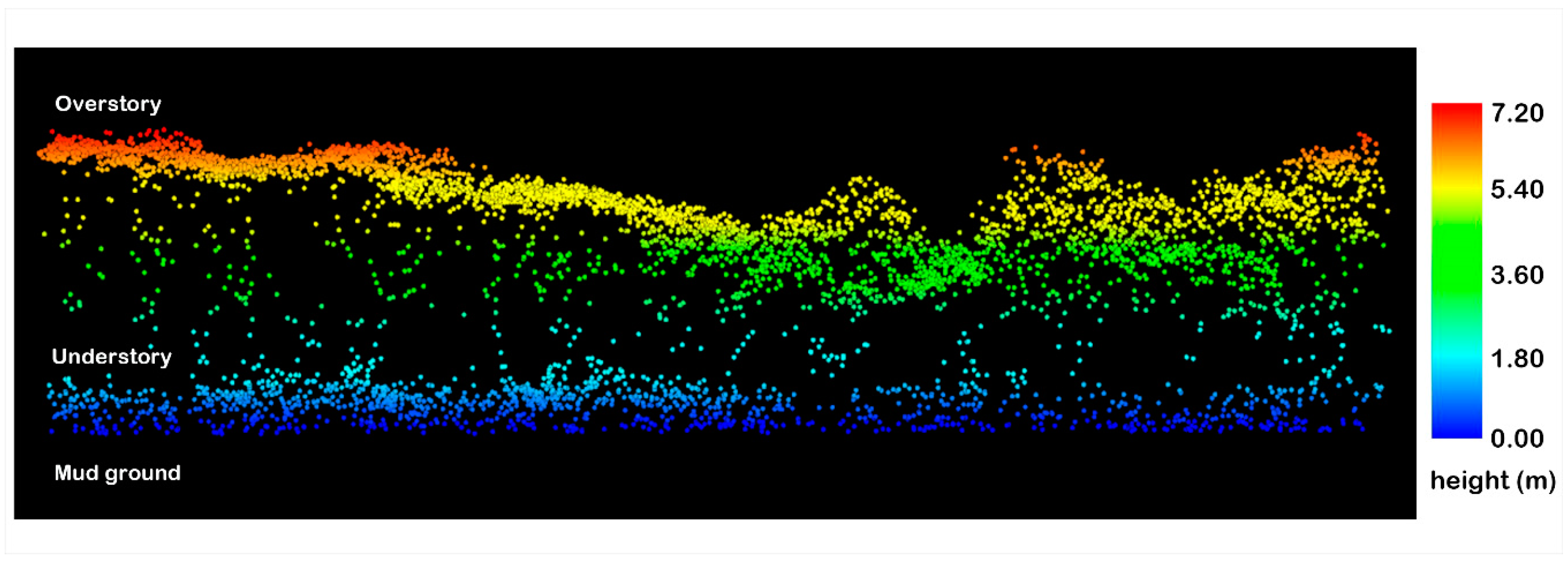
The LiDAR data were also registered to align with the digital aerial orthophotos. A filtering method, Progressive Triangular Irregular Network (TIN) Densification, devised by Axelsson [30] was applied to the LiDAR point cloud to classify ground and non-ground points. LiDAR data was preprocessed by using LAStools (http://cs.unc.edu/~isenburg/lastools/). Figure 2 showed an example of the vertical profile of the mangroves in LiDAR point cloud. LiDAR metrics were generated in a 2 m and 5 m resolution for comparison purpose.
2.3. Field Survey and Reference Data Collection
Species distribution surveys were conducted during March and May in 2018 when Aegiceras corniculatum (AC) blossomed. The presence of flowers improved the certainty and efficiency in distinguishing different species. The mangroves were accessed by a floating boardwalk and by a boat from south to north along the mangrove edge in the Deep Bay. A 5 m accuracy GPS was used to measure the location of in situ samples. Site photos and tree heights were also recorded. According to the site survey, Kandelia obovata (KO) and Avicennia marina (AM) were the two dominant overstory species. Acanthus ilicifolius (AI) was mainly distributed as pioneer species along coastal edges or as understory in the middle part of the study area. AC was frequently found at the edges of seaside and waterway. Exotic species Sonneratia apetala (SA) was sporadically found at coastal edges.
As most of the study area is swampy and inaccessible, extra sample data were collected by visual interpretation from the WV-3 pan-sharpened image aided by experience from field survey. The mangrove species were classified into seven classes. Specifically, the species of KO was sub-classified into two types based on their significant difference in crown shape and spectral information. One group was identified as pure KO with dense canopy crown and the other group was noted as a mixture of KO and AI in which the canopy crown of KO is relatively small and sparse while understory AI is dense. A total of 245 samples were selected from the study area as shown in Figure 1 and these samples were randomly partitioned into training and testing samples in the ratio of 7:3. Species classes and sample size are described in Table 2.
2.4. Feature Generation and Selection
Feature selection algorithms are able to identify important features, reduce data redundancy, and increase the model interpretability, meanwhile improving the speed and accuracy in training as well as in classification [7,21]. To this end, feature selection was performed with recursive feature elimination (RFE) based on the Random Forest (RF) model in this study. Recursive feature elimination is a backward selection algorithm which inputs all features to fit a random forest model at the beginning and returns the ranking of feature importance. At each iteration, top-ranked features are retained to train the model. A performance profile is created to summarize all the iterations so that an optimal subset can be determined and the ranking of features is returned.
In order to explore the spectral region and optimal spatial resolution for distinguishing mangrove species, both the WV-3 MS image and pan-sharpened image were used and the eight bands of both images were input as spectral data for feature selection.
Various LiDAR metrics derived from point cloud elevation describe tree structure characteristics, which were widely applied in tree classification, crown segmentation and biophysical parameter retrieval [19,31]. In order to get meaningful metrics, grid size was suggested to be larger than individual tree crowns. Since the diameter of most of the canopy crowns is less than 5 m, some are even less than 2 m, and the presence of mixed species in some area, a fine-scale grid was more likely to include pure species in each grid. Therefore, a 2 m-grid size which is compatible with the WV-2 MS image resolution and a 5 m-grid size were designed to explore the optimal LiDAR metric resolution for mangrove species classification. AI was observed as the dominant understory species and their canopy height ranged from 0.48 m to 1.62 m as measured in the field survey. Therefore, the height threshold to separate overstory and understory was set to 1.8 m in LiDAR metrics computation. 57 elevation metrics were generated by all returns of LiDAR point cloud in 2 m and 5 m cell size respectively in Fusion software (http://forsys.cfr.washington.edu/fusion/fusion_overview.html). The description of 57 elevation metrics is provided in Appendix A Table A1.
Feature selection was processed in R project (https://www.r-project.org/) with package “Caret”. The 10-fold cross validation was applied to evaluate the model performance by overall accuracy and Kappa. Feature selection was performed with WV-3 data and LiDAR metrics separately. The selected features were then combined to ascertain the effectiveness of spectral and structural features in mangrove species discrimination and identification.
2.5. Classification and Validation
Machine learning classifiers such as Support Vector Machine (SVM) and Random Forest (RF) were successfully applied in vegetation classification studies using remote sensing data [32,33]. In the present study, these two supervised classification algorithms were compared for their performance in classifying mangrove species.
2.5.1. Support Vector Machine Classifier
The SVM classifier is based on the statistical learning theory of structural risk minimization (SRM) to improve classification performance. A kernel-based SVM essentially performs the classification by transforming from the original multi-dimension in which the problem is inseparable to a linearly separated higher-dimension through the kernel function. Support vectors are searched to construct a hyperplane with the maximum margin to separate different classes [34]. Radial basis function (RBF) kernel is used to map samples to higher-dimensional space nonlinearly which better handles reality circumstances [35]. Two parameters, cost of constraint violation (C) and sigma (σ), are used to control the overfitting and shape hyperplane respectively during classifier training. In this study, various pairs of C and sigma (σ) with a setting range of 10−3–10+3 were searched with 10-fold cross validation to determine the best tuning parameters in R project with the “e1071” package.
2.5.2. Random Forest Classifier
RF is an ensemble learning method for classification. It operates by using different bootstrap samples originating from the training data to grow each decision tree. For each node, a subset of input features (Mtry) is randomly selected for searching the best split. When a test sample is input, each tree gives a classification result and the forest chooses the majority voting as the final classification result [36]. In this study, the parameter Mtry was tuned with a range from 2 to the number of input features by 10-fold cross validation carrying out in R project with the “randomForest” package.
2.5.3. Validation
After using training samples to train models, testing samples were input to model for species identification. Classification accuracy was assessed by overall accuracy (OA) and Kappa coefficient for the entire dataset, whilst user‘s accuracy (UA) and producer’s accuracy (PA) were computed for individual classes.
3. Results
3.1. Feature Selection
Table 3 summarizes the feature selection result of each data. When WV-3 spectral bands were the only inputs for feature selection, the selected features of the original 2 m MS image and the 0.5 m pan-sharpened image were similar. For the original 2 m MS image, seven bands were selected except the coastal blue bands (B1), while for the 0.5 m pan-sharpened image, all of eight bands were selected. Both results showed similar feature importance. The green band (B3) and red edge band (B6) were identified as the most important features followed by the yellow band (B4), red band (B5) and NIR band (B7). The blue band (B2), extra NIR2 band (B8), and coastal blue band (B1) were, however, considered as less important in distinguishing mangrove species. Differences of WV-3 bands’ value among species are shown in Figure 3, KO and KOAI were very similar in visible bands but KO had a much higher spectral reflectance than KOAI in the red edge band (B6) and NIR bands (B7 and B8). A few pairs of classes were hard to be differentiated. For instance, AC and AI tended to have very similar spectral reflectance in most bands but the green band (B3) might be able to contribute some information. Grass and AM showed great difference from other species in the red band (B5).
When the LiDAR elevation metrics were input for feature selection, the results showed a slight difference between the 2 m-grid metrics versus the 5 m-grid metrics. 10 metrics were retained from the 2 m-grid metrics while eight metrics were selected from the 5 m-grid metrics. Six metrics were commonly selected including canopy height model (CHM), standard deviation of elevation (Elev stddev), variance of elevation (Elev var), canopy relief ratio, absolute average deviation of elevation (Elev AAD) and Elevation L2 (Elev L2). In the 2 m-grid, metrics 99th and 95th percentile height (Elev P99 and Elev P95), mean and median of elevation were also considered important. Additionally, skewness of elevation (Elev.skewness) and the number of returns above the mean height/number of total first returns × 100 ((All returns above mean)/(Total first returns) × 100) were chosen from the 5 m-grid metrics. Figure 4 describes the difference among species in the 10 important LiDAR metrics.
In order to determine the best resolution, the optimal feature subsets were input to train the classifiers and assess the classification accuracy. As shown in Table 3, 2 m resolution WV-3 image produced higher OA (0.70 for RF, 0.72 for SVM) than 0.5 m fused image (0.68 for RF and SVM). Similarly, 2 m LiDAR metrics produced slightly higher OA (0.79) than 5 m LiDAR metrics (0.78) using both SVM and RF classifiers. Therefore, 2 m resolution features were subsequently combined for feature selection. 14 features were selected from the combined dataset including eight LiDAR elevation metrics and six spectral bands. Feature selection result showed that LiDAR features were more important than spectral features as the top five selected features were all LiDAR metrics followed by the red edge band (B6). The other five bands were regarded as less important features.
The optimal subset sizes ranged from 7 to 14 based on all feature selection exercises, which was consistent with previous studies [7,21]. Figure 5 shows the variation of overall accuracy and Kappa generated from the RFE RF model with changes in the number of features used in the combined data. Overall accuracy and Kappa coefficient kept increasing when the number of features increased. The improvement is more significant when the subset sizes were less than 10. When beyond 10 features, the improvement was dampened and revealed a trend of gradual saturation between 11 to 15 features. In this example, the highest overall accuracy (0.91) and Kappa (0.89) were achieved with 14 features used. When the subset size was larger than 15, Kappa coefficient saturated and showed a decline with more features added.
3.2. Classification and Validation
Table 4 shows the confusion matrix together with the overall accuracy and Kappa yielded by different classifiers when the classification was performed with WV-3 data only. SVM (OA = 0.72 with Kappa = 0.66) performed slightly better than RF (OA = 0.70 with Kappa = 0.63).
Classification results from using only the LiDAR data showed that SVM and RF produced nearly similar overall accuracy at 0.79 with Kappa coefficient at 0.74 and 0.75 respectively (Table 5). Specifically, RF yielded higher PA in AC, grass, KO, and SA while SVM yielded higher PA in AI and AM.
With the combined data, both SVM and RF obtained similar results. OA and Kappa were 0.88 and 0.85 for the SVM classifier and 0.87 and 0.85 for the RF classifier. As shown in Table 6, SVM identified AI and SA better than RF while RF outperformed SVM in identifying AC.
In comparison of the data source, LiDAR data outperformed WV-3 images. AC, AI, and AM were not accurately mapped when using the WV-3 data only. AC only obtained around 0.2 of PA and was largely misclassified to AI, AM, and KO. AI were misclassified as AC. AM only obtained about 0.65 of PA. Approximately 40% of AM were misclassified as KOAI. The presence of gaps and shadows might have affected the spectral reflectance of AM. Meanwhile, training samples of KOAI also included the gap between KO and AI. Therefore, there is a higher chance of misclassification result if spectral reflectance was considered alone.
The LiDAR data is able to differentiate the three mixed species AC, AI, and AM as the PA were improved to around 0.5, 0.8, and 0.9 respectively. However, the PA of grass and SA declined to 0.5. Low shrub vegetation such as grass and AI were mixed due to similar heights. The same problem was observed in exotic SA, KO, and AM with similar height.
Compared to the two independent data, the combined feature dataset significantly enhanced the PA and UA of most of the species. KO and KOAI yielded over 90% PA and UA using SVM and RF algorithms. Among the species, AC yielded the lowest PA and UA. Figure 6 shows the RF classified maps using WV-3 data, LiDAR data, combined data, and the false color WV-3 image is for reference. As shown in Figure 6b, using spectral data alone tends to produce more scattered species pixels than the one using LiDAR data alone (Figure 6c). Based on visual analysis, areas of AC and AI were underestimated in Figure 6b but overestimated in Figure 6c. Combining both data improved the identification of AC and AI. Additionally, shadow influence along the coastal and salt and pepper effect were significantly reduced with the combined data.
4. Discussion
In this study, important spectral bands of WV-3 and crown structure features derived from airborne LiDAR were used for mangrove species classification in Mai Po Ramsar site in Hong Kong. Two machine learning algorithms, SVM and RF, were applied to examine the capacity of the selected spectral, structure features and their combination in mangrove species classification. The result revealed that both classifiers made the best of combined features for mangrove species classification yielding the highest OA at 0.88 comparing to using WV-3 (OA at around 0.70) and LiDAR (OA at 0.79), individually.
The recursive feature elimination based on RF selected a series of important features and determined the optimal feature subset size for each data. Feature selection results suggested useful bands of WV-3 in differentiating the species including the green, red edge, red, yellow, NIR1, blue, and NIR2 bands. The two most important bands, green and red edge, were sensitive to the concentration of the chlorophyll [37] and were controlled by the leaf internal scattering [38], respectively. The red and blue bands were absorption peaks of chlorophyll for photosynthesis, which clearly separated grass from the mangrove species. The yellow band reflected non-green pigments, such as carotenoids and xanthophyll in leaf. Last but not least, although both two NIR bands were dominantly controlled by the cellular structure within the leaf and sensitive to moisture content [39,40], NIR1 was considered more useful than NIR2 because NIR1 is able to tell apart the AM, KO, and grass.
Therefore, spectral bands that are able to reveal differences in pigment, chemical compounds and leaf internal structure among species are useful. This echos the results found in previous studies. However, species have similar pigment contents, and the leaf internal structure is hard to be differentiated using spectral data alone. As demonstrated by this study, species such as AC, AI, and AM share similar spectral reflectance.
Canopy height and crown shape were good indicators for vegetation species classification [18,19] and this study shows similar results. As shown in Figure 4, LiDAR metrics describing canopy height such as CHM, cubic mean of elevation, 95th percentile, and 95th percentile of the elevation were selected as useful metrics because AI and grass can easily be separated from arbor species. Meanwhile, the height of KO was generally taller than that of AM and SA. Hence, important LiDAR metrics describing the variability of LiDAR point elevation including standard deviation of elevation, variance of elevation, and median of elevation, which reflected canopy shape and vertical stratification was identified. For example, canopies of KO and AM were sparse and more open, and so LiDAR pulses can hit the understory of AI directly through gaps and generated returns from lower elevation. Therefore, the variability of canopy height in KOAI and AM samples were larger than other species with dense canopies. For another example, the exotic SA is usually clustered in groups or as an isolated tree among a patch of pure species which is characterized by the flat canopy such as pure KO and AC. Canopy relief ratio as a descriptor of crown shape from altimetry observation reflected the canopy surfaces that were in the upper or lower portion of the height range. Both [38,41] indicated the importance of vertical stratification of samples. Thus, single canopy layer of AI, grass, and KO obtained extreme values in canopy relief ratio. Shi et al. and Liu et al. found LiDAR data acquired in leaf-off or semi-leaf-on period interacted more with upper canopy and the spatial characteristics of trunk and branch, and thus could be better described [17,19]. Likewise, although mangrove was evergreen vegetation in our study site, the majority of the upper canopies of mangrove were sparse in Mai Po. Therefore, LiDAR structure metrics possessed important information and could classify species with similar spectral characteristics. From the above discussion, the combined data made a complimentary use of spectral and spatial structure features and produced the best accuracy.
The classified map of WV-3 data (Figure 6b) is more scattered than classified maps of LiDAR (Figure 6c) and combined data (Figure 6d). In the study area, the upper mangrove canopies are relatively sparse resulting in a lot of little gaps and shadows appearing in the WV-3 image, which can affect the mangrove canopy reflectance and lead to a mix of canopy and gap/shadow pixels in the classified maps. The canopy heights derived from the first LiDAR return produces a much smoother canopy surface and areas of same species tend to produce a more aggregated result. While there is a difference in canopy height of two species, the boundary is very distinctive. The classified map of WV-3 data (Figure 6b) showed an underestimation on AC. Among the species, AC and KO were hard to discriminate either in fieldwork or through visual interpretation as they have very similar spectral properties and physical appearance. Besides, the areal coverage of AC is relatively small while KO is the dominant species. Hence, reliable training samples of AC was far less than that of KO. The sole use of WV-3 image is not able to separate AC from KO. From fieldwork experience, the canopy height of mature KO is taller than that of AM and AC. This is also revealed by the CHM metric in Figure 4. The average canopy heights of KO, AM, and AC were 6.57, 5.18, and 3.36 m respectively. Hence, species with low canopy height were classified as AC in LiDAR data.
The comparative analysis of spatial resolution demonstrated that at 2 m resolution, both WV-3 and LiDAR data were suitable for pixel-based classification. In terms of WV-3 data, the pan-sharpening process changed the original spectral information to some degree which might affect true spectral characteristics of the species. Meanwhile, many studies indicated that object-based classification outperformed pixel-based classification for very high-resolution image [2,7]. However, it was challenging to apply an object segmentation in this study as different mangrove species would be mixed together and grew to patches of flat canopy surface. It is also found that high return density LiDAR enabled meaningful metrics to be derived in finer grid size. The 5 m-grid metrics attained marginally lower accuracy than 2 m-grid metrics. The integration of WV-3 and LiDAR data at the same 2 m spatial resolution also provided the most accurate classification result.
Previous studies found that SVM outperformed RF [7,32,33]. In this study, both classifiers obtained nearly similar overall accuracy and kappa when the combined dataset was used. However, the two classifiers showed their respective advantages in identifying various species. For SVM, it obtained more obvious improvement in classifying AI and SA using the combined data. RF used bootstrap samples to grow each decision tree, which was less sensitive to outliners. It should be noted that there were limited samples for some species (e.g., AC, SA, grass) in the study site. RF randomly selected a subset of features to search for the best split for nodes which enabled RF to handle collinear features better. In terms of computation efficiency, RF was more efficient than SVM because SVM needed more computation time in grid search in order to find the best parameter pairs.
5. Conclusions
This study compared single WV-3 image, LiDAR data and the combined dataset in classifying six mangrove species in the Mai Po Nature Reserve. The result demonstrated that the combined data can effectively identify and map the species and obtained better accuracy than previous studies in the same area [6,42,43]. The identification of species Aegiceras corniculatum (AC) and Avicennia marina (AM) was greatly improved when compared with using WV-3 or LiDAR data alone. Important features were selected from the spectral and LiDAR data using recursive feature elimination (RFE) based on the Random Forest (RF) model. The red edge and green band followed by the red, yellow and NIR were considered as useful spectral bands. LiDAR elevation metrics describing crown characteristics from three aspects, canopy height, variation of canopy surface, and canopy stratification were selected as important canopy structure features. It also revealed that the LiDAR structural features were more important than spectral data for discrimination between the mangrove species. In terms of image classification, this study found RF algorithm is more effective in handling the combined data set as compared to SVM.
The significance of this study could be addressed in two aspects. First, distribution of mangrove species was mapped with high accuracy, which may assist the government official to monitor and conserve the mangrove habitats, and prevent the extent of the invasion of exotic species such as SA. Secondly, the combined data showed great potential not only in identifying mangrove species, but also in describing the vertical stratification which is not available before. However, some challenges should be addressed in future studies. In this study, LiDAR crown shape and structure descriptors, as well as LiDAR intensity metrics, had not been fully explored for classification. Besides, the data can contribute to the estimation of other biophysical parameters and evaluation of ecosystem service.
Author Contributions
Study design, fieldwork investigation, data analysis and writing—original draft preparation, Q.L.; study design, providing useful suggestion on data and result analysis, writing—review and editing, F.K.K.W.; providing useful suggestion on data and result analysis, writing—review and editing, supervision, T.F.
Funding
This research was funded by a Hong Kong Research Grant Council General Research Grant Project No. 14618715.
Acknowledgments
Fieldwork assistance provided by Thomas Lui and Jack Cheng was deeply appreciated.
Conflicts of Interest
The authors declare no conflict of interest.
Appendix A

Table A1.
LiDAR elevation metrics derived LiDAR data.
| Abbreviation of LiDAR Metric | Explanation |
|---|---|
| Elev minimum | Elevation minimum |
| CHM | Canopy height model |
| Elev mean | Elevation mean |
| Elev mode | Elevation mode |
| Elev stddev | Elevation standard deviation |
| Elev variance | Elevation variance |
| Elev CV | Elevation coefficient of variation |
| Elev IQ | Elevation 75th percentile minus 25th percentile |
| Elev skewness | Elevation skewness |
| Elev kurtosis | Elevation kurtosis |
| Elev AAD | Elevation average absolute deviation from mean |
| Elev L1, Elev L2,Elev L3,Elev L4 | Elevation L-moments (L1, L2, L3, L4) |
| Elev L CV | Elevation L-moments coefficient of variation |
| Elev L skewness | Elevation L-moments skewness |
| Elev L kurtosis | Elevation L-moments kurtosis |
| Elev P01, Elev P05, Elev 10, Elev P20, Elev P25, Elev P30, Elev P40, Elev P50, Elev P60, Elev P70, Elev P75, Elev P80, Elev 90, Elev P95, Elev P99 | 1st, 5th, 10th 20th, 25th, 30th, 40th, 50th, 60th, 70th, 75th, 80th, 90th, 95th, 99th percentile of elevation |
| Return 1 count | Count of return 1 points |
| Return 2 count | Count of return 2 points |
| canopy cover estimate | Percentage first returns above 1.8 m |
| Percentage all returns above 1.8 | Percentage all returns above 1.8 m |
| (All returns above 1.8)/(Total first returns) × 100 | (All returns above 1.8)/(Total first returns) × 100 |
| First returns above 1.8 | First returns above 1.8 m |
| All returns above 1.8 | All returns above 1.8 m |
| Percentage first returns above mean | Percentage first returns above mean |
| Percentage first returns above mode | Percentage first returns above mode |
| Percentage all returns above mean | Percentage all returns above mean |
| Percentage all returns above mode | Percentage all returns above mode |
| Number of returns above the mean height Number of total first returns × 100 | (All returns above mean)/(Total first returns) × 100 |
| Number of returns above the mode height/Number of total first returns × 100 | (All returns above mode)/(Total first returns) × 100 |
| First returns above mean | First returns above mean |
| First returns above mode | First returns above mode |
| All returns above mean | All returns above mean |
| All returns above mode | All returns above mode |
| Total first returns | Total first returns |
| Total all returns | Total all returns |
| Elev MAD median | Elevation median absolute deviation from the median |
| Elev MAD mode | Elevation median absolute deviation from the mode |
| Canopy relief ratio | Elevation (mean-min)/(max–min) |
| Elev quadratic mean | Elevation quadratic mean |
| Elev cubic mean | Elevation cubic mean |
References
- Tam, N.F.Y.; Wong, Y.-S. Hong Kong Mangroves; City University of Hong Kong Press: Hong Kong, China, 2000; ISBN 9629370557. Available online: https://julac.hosted.exlibrisgroup.com/primo-explore/fulldisplay?docid=CUHK_IZ21810919350003407&context=L&vid=CUHK&lang=en_US&search_scope=Books&adaptor=Local Search Engine&tab=default_tab&query=any,contains, HONG KONG Mangroves&sortby=rank (accessed on 11 September 2019).
- Heenkenda, M.; Joyce, K.; Maier, S.; Bartolo, R. Mangrove Species Identification: Comparing WorldView-2 with Aerial Photographs. Remote Sens. 2014, 6, 6064–6088. [Google Scholar] [CrossRef] [Green Version]
- Heumann, B.W. Satellite remote sensing of mangrove forests: Recent advances and future opportunities. Prog. Phys. Geogr. 2011, 35, 87–108. [Google Scholar] [CrossRef]
- Neukermans, G.; Dahdouh-Guebas, F.; Kairo, J.G.; Koedam, N. Mangrove species and stand mapping in Gazi bay (Kenya) using quickbird satellite imagery. J. Spat. Sci. 2008, 53, 75–86. [Google Scholar] [CrossRef]
- Wang, L.; Sousa, W.P.; Gong, P.; Biging, G.S. Comparison of IKONOS and QuickBird images for mapping mangrove species on the Caribbean coast of Panama. Remote Sens. Environ. 2004, 91, 432–440. [Google Scholar] [CrossRef]
- Wang, T.; Zhang, H.; Lin, H.; Fang, C. Textural–Spectral Feature-Based Species Classification of Mangroves in Mai Po Nature Reserve from Worldview-3 Imagery. Remote Sens. 2015, 8, 24. [Google Scholar] [CrossRef]
- Ghosh, A.; Joshi, P.K. A comparison of selected classification algorithms for mapping bamboo patches in lower Gangetic plains using very high resolution WorldView 2 imagery. Int. J. Appl. Earth Obs. Geoinf. 2014, 26, 298–311. [Google Scholar] [CrossRef]
- Immitzer, M.; Atzberger, C.; Koukal, T. Tree Species Classification with Random Forest Using Very High Spatial Resolution 8-Band WorldView-2 Satellite Data. Remote Sens. 2012, 4, 2661–2693. [Google Scholar] [CrossRef] [Green Version]
- Sothe, C.; de Almeida, C.M.; Schimalski, M.B.; Liesenberg, V. Integration of Worldview-2 and Lidar Data to MAP a Subtropical Forest Area: Comparison of Machine Learning Algorithms. In Proceedings of the IGARSS 2018—IEEE International Geoscience and Remote Sensing Symposium, Valencia, Spain, 22–27 July 2018; pp. 6207–6210. [Google Scholar]
- Tian, J.; Wang, L.; Li, X.; Gong, H.; Shi, C.; Zhong, R.; Liu, X. Comparison of UAV and WorldView-2 imagery for mapping leaf area index of mangrove forest. Int. J. Appl. Earth Obs. Geoinf. 2017, 61, 22–31. [Google Scholar] [CrossRef]
- Zhang, Z.; Liu, X. WorldView-2 Satellite Imagery and Airborne LiDAR Data for Object-Based Forest Species Classification in a Cool Temperate Rainforest Environment. In Developments in Multidimensional Spatial Data Models; Springer: Berlin/Heidelberg, Germany, 2013; pp. 103–122. Available online: http://link.springer.com/10.1007/978-3-642-36379-5_7 (accessed on 11 September 2019).
- Zhu, Y.; Liu, K.; Liu, L.; Myint, S.; Wang, S.; Liu, H.; He, Z.; Zhu, Y.; Liu, K.; Liu, L.; et al. Exploring the Potential of WorldView-2 Red-Edge Band-Based Vegetation Indices for Estimation of Mangrove Leaf Area Index with Machine Learning Algorithms. Remote Sens. 2017, 9, 1060. [Google Scholar] [CrossRef]
- Luo, S.; Wang, C.; Pan, F.; Xi, X.; Li, G.; Nie, S.; Xia, S. Estimation of wetland vegetation height and leaf area index using airborne laser scanning data. Ecol. Indic. 2015, 48, 550–559. [Google Scholar] [CrossRef]
- Hamraz, H.; Contreras, M.A.; Zhang, J. Vertical stratification of forest canopy for segmentation of understory trees within small-footprint airborne LiDAR point clouds. ISPRS J. Photogramm. Remote Sens. 2017, 130, 385–392. [Google Scholar] [CrossRef] [Green Version]
- Cao, L.; Coops, N.C.; Innes, J.L.; Sheppard, S.R.J.; Fu, L.; Ruan, H.; She, G. Estimation of forest biomass dynamics in subtropical forests using multi-temporal airborne LiDAR data. Remote Sens. Environ. 2016, 178, 158–171. [Google Scholar] [CrossRef]
- Dalponte, M.; Bruzzone, L.; Gianelle, D. Tree species classification in the Southern Alps based on the fusion of very high geometrical resolution multispectral/hyperspectral images and LiDAR data. Remote Sens. Environ. 2012, 123, 258–270. [Google Scholar] [CrossRef]
- Shi, Y.; Wang, T.; Skidmore, A.K.; Heurich, M. Important LiDAR metrics for discriminating forest tree species in Central Europe. ISPRS J. Photogramm. Remote Sens. 2018, 137, 163–174. [Google Scholar] [CrossRef]
- Jones, T.G.; Coops, N.C.; Sharma, T. Assessing the utility of airborne hyperspectral and LiDAR data for species distribution mapping in the coastal Pacific Northwest, Canada. Remote Sens. Environ. 2010, 114, 2841–2852. [Google Scholar] [CrossRef]
- Liu, L.; Coops, N.C.; Aven, N.W.; Pang, Y. Mapping urban tree species using integrated airborne hyperspectral and LiDAR remote sensing data. Remote Sens. Environ. 2017, 200, 170–182. [Google Scholar] [CrossRef]
- Chadwick, J. Integrated LiDAR and IKONOS multispectral imagery for mapping mangrove distribution and physical properties. Int. J. Remote Sens. 2011, 32, 6765–6781. [Google Scholar] [CrossRef]
- Fassnacht, F.E.; Neumann, C.; Forster, M.; Buddenbaum, H.; Ghosh, A.; Clasen, A.; Joshi, P.K.; Koch, B. Comparison of Feature Reduction Algorithms for Classifying Tree Species With Hyperspectral Data on Three Central European Test Sites. IEEE J. Sel. Top. Appl. Earth Obs. Remote Sens. 2014, 7, 2547–2561. [Google Scholar] [CrossRef]
- Pal, M.; Foody, G.M. Feature Selection for Classification of Hyperspectral Data by SVM. IEEE Trans. Geosci. Remote Sens. 2010, 48, 2297–2307. [Google Scholar] [CrossRef] [Green Version]
- Guyon, I.; Elisseeff, A. An Introduction to Variable and Feature Selection. J. Mach. Learn. Res. 2003, 3, 1157–1182. [Google Scholar]
- Cheng, Q.; Varshney, P.K.; Arora, M.K. Logistic Regression for Feature Selection and Soft Classification of Remote Sensing Data. IEEE Geosci. Remote Sens. Lett. 2006, 3, 491–494. [Google Scholar] [CrossRef]
- Tang, Y.; Jing, L.; Li, H.; Liu, Q.; Yan, Q.; Li, X. Bamboo Classification Using WorldView-2 Imagery of Giant Panda Habitat in a Large Shaded Area in Wolong, Sichuan Province, China. Sensors 2016, 16, 1957. [Google Scholar] [CrossRef] [PubMed]
- Richardson, J.J.; Moskal, L.M.; Kim, S.-H. Modeling approaches to estimate effective leaf area index from aerial discrete-return LIDAR. Agric. For. Meteorol. 2009, 149, 1152–1160. [Google Scholar] [CrossRef]
- WWF Hong Kong Mai Po Nature Reserve | WWF Hong Kong. Available online: https://www.wwf.org.hk/en/whatwedo/water_wetlands/mai_po_nature_reserve/ (accessed on 29 May 2019).
- AFCD Agriculture, Fisheries and Conservation Department. Available online: https://www.afcd.gov.hk/english/conservation/con_wet/con_wet_look/con_wet_look_gen/con_wet_look_gen.html (accessed on 29 May 2019).
- Waser, L.; Küchler, M.; Jütte, K.; Stampfer, T.; Waser, L.T.; Küchler, M.; Jütte, K.; Stampfer, T. Evaluating the Potential of WorldView-2 Data to Classify Tree Species and Different Levels of Ash Mortality. Remote Sens. 2014, 6, 4515–4545. [Google Scholar] [CrossRef] [Green Version]
- Axelsson, P. DEM generation from laser scanner data using adaptive TIN models. Int. Arch. Photogram. Remote Sens. 2000, 33, 110–117. [Google Scholar]
- Lagomasino, D.; Fatoyinbo, T.; Lee, S.; Feliciano, E.; Trettin, C.; Simard, M. A Comparison of Mangrove Canopy Height Using Multiple Independent Measurements from Land, Air, and Space. Remote Sens. 2016, 8, 327. [Google Scholar] [CrossRef] [PubMed]
- Ballanti, L.; Blesius, L.; Hines, E.; Kruse, B. Tree Species Classification Using Hyperspectral Imagery: A Comparison of Two Classifiers. Remote Sens. 2016, 8, 445. [Google Scholar] [CrossRef]
- Raczko, E.; Zagajewski, B. Comparison of support vector machine, random forest and neural network classifiers for tree species classification on airborne hyperspectral APEX images. Eur. J. Remote Sens. 2017, 50, 144–154. [Google Scholar] [CrossRef] [Green Version]
- Mountrakis, G.; Im, J.; Ogole, C. Support vector machines in remote sensing: A review. ISPRS J. Photogramm. Remote Sens. 2011, 66, 247–259. [Google Scholar] [CrossRef]
- Fan, R.-E.; Chen, P.-H.; Lin, C.-J. Working Set Selection Using Second Order Information for Training Support Vector Machines. J. Mach. Learn. Res. 2005, 6, 1889–1918. [Google Scholar]
- Breiman, L. Random Forests. Mach. Learn. 2001, 45, 5–32. [Google Scholar] [CrossRef] [Green Version]
- Gitelson, A.A.; Kaufman, Y.J.; Merzlyak, M.N. Use of a green channel in remote sensing of global vegetation from EOS-MODIS. Remote Sens. Environ. 1996, 58, 289–298. [Google Scholar] [CrossRef]
- Pike, R.J.; Wilson, S.E. Elevation-Relief Ratio, Hypsometric Integral, and Geomorphic Area-Altitude Analysis. Geol. Soc. Am. Bull. 1971, 82, 1079–1084. [Google Scholar] [CrossRef]
- DigitalGlobe. The Benefits of the Eight Spectral Bands of WORLDVIEW-2. Available online: www.digitalglobe.com (accessed on 29 May 2019).
- Peñuelas, J.; Filella, I. Visible and near-infrared reflectance techniques for diagnosing plant physiological status. Trends Plant Sci. 1998, 3, 151–156. [Google Scholar] [CrossRef]
- Parker, G.G.; Russ, M.E. The canopy surface and stand development: Assessing forest canopy structure and complexity with near-surface altimetry. For. Ecol. Manag. 2004, 189, 307–315. [Google Scholar] [CrossRef]
- Jia, M.; Zhang, Y.; Wang, Z.; Song, K.; Ren, C. Mapping the distribution of mangrove species in the Core Zone of Mai Po Marshes Nature Reserve, Hong Kong, using hyperspectral data and high-resolution data. Int. J. Appl. Earth Obs. Geoinf. 2014, 33, 226–231. [Google Scholar] [CrossRef]
- Wong, F.K.K.; Fung, T. Combining EO-1 Hyperion and Envisat ASAR data for mangrove species classification in Mai Po Ramsar Site, Hong Kong. Int. J. Remote Sens. 2014, 35, 7828–7856. [Google Scholar] [CrossRef]
Figure 1.
Map of the study area and the distribution of ground truth samples.
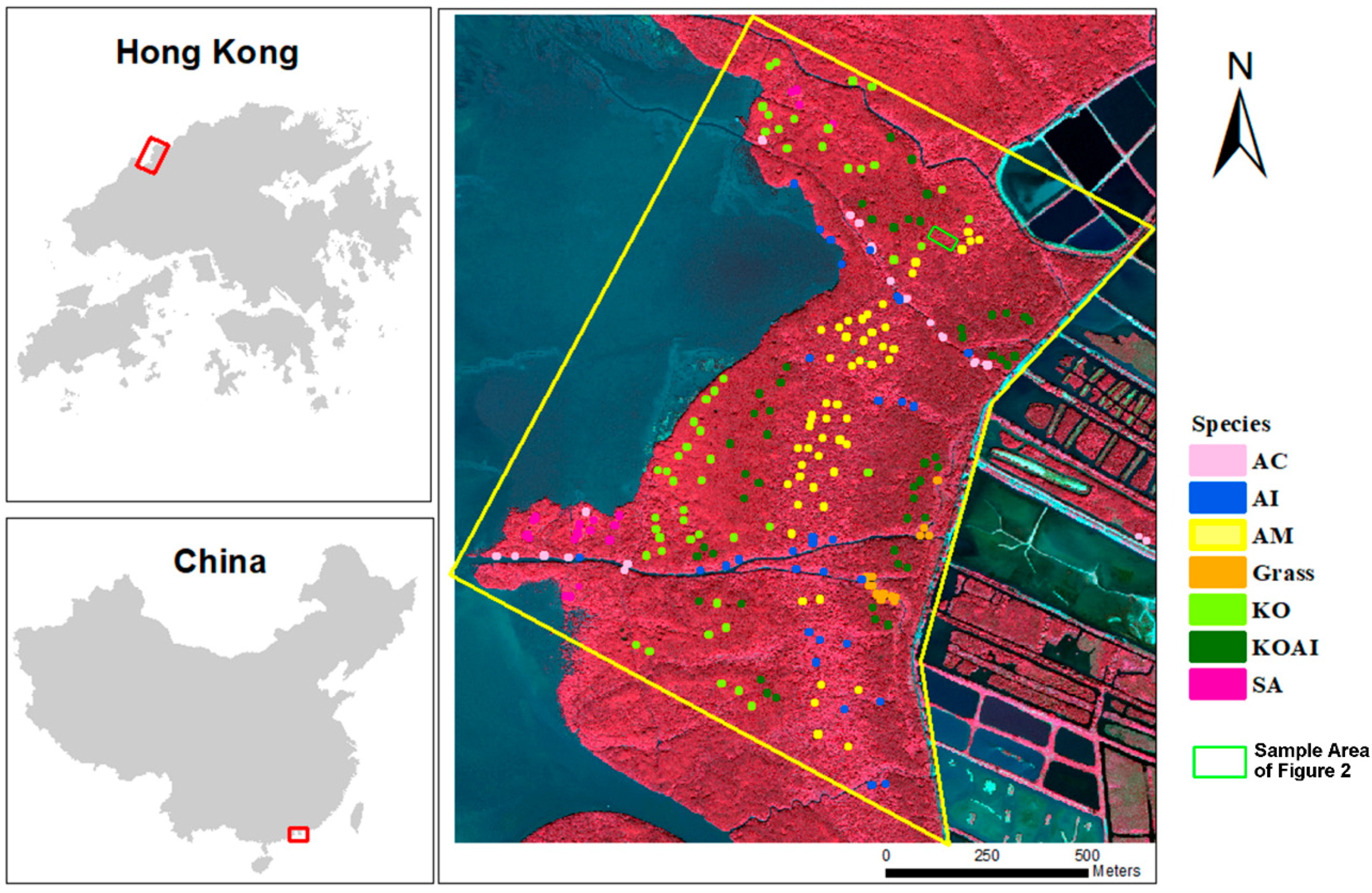
Figure 2.
Illustration of mangrove vertical profile produced from LiDAR data in the study area. The LiDAR point cloud is displayed by height and the location of sample area is shown in Figure 1.
Figure 2.
Illustration of mangrove vertical profile produced from LiDAR data in the study area. The LiDAR point cloud is displayed by height and the location of sample area is shown in Figure 1.

Figure 3.
Difference among species in WV-3 MS bands value (B1: coastal blue band, B2: blue band, B3: green band, B4: yellow band, B5: red band, B6: red edge band, B7: NIR1 band, and B8: NIR2 band).
Figure 3.
Difference among species in WV-3 MS bands value (B1: coastal blue band, B2: blue band, B3: green band, B4: yellow band, B5: red band, B6: red edge band, B7: NIR1 band, and B8: NIR2 band).
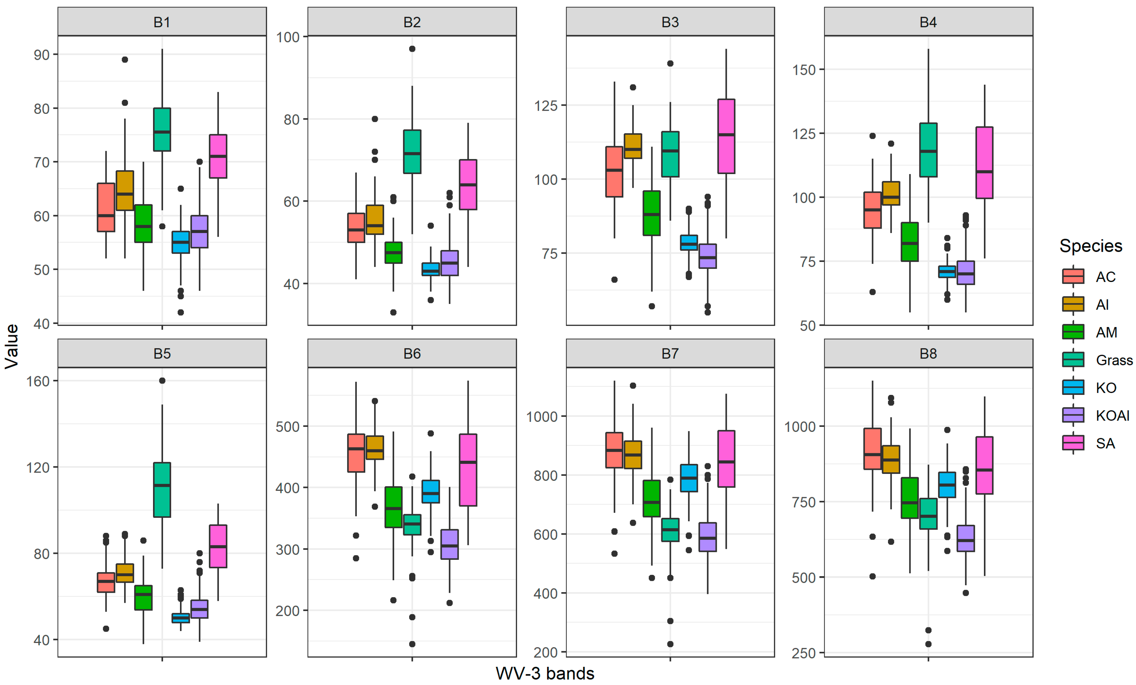
Figure 4.
Difference among species in 2 m-grid LiDAR elevation metrics.
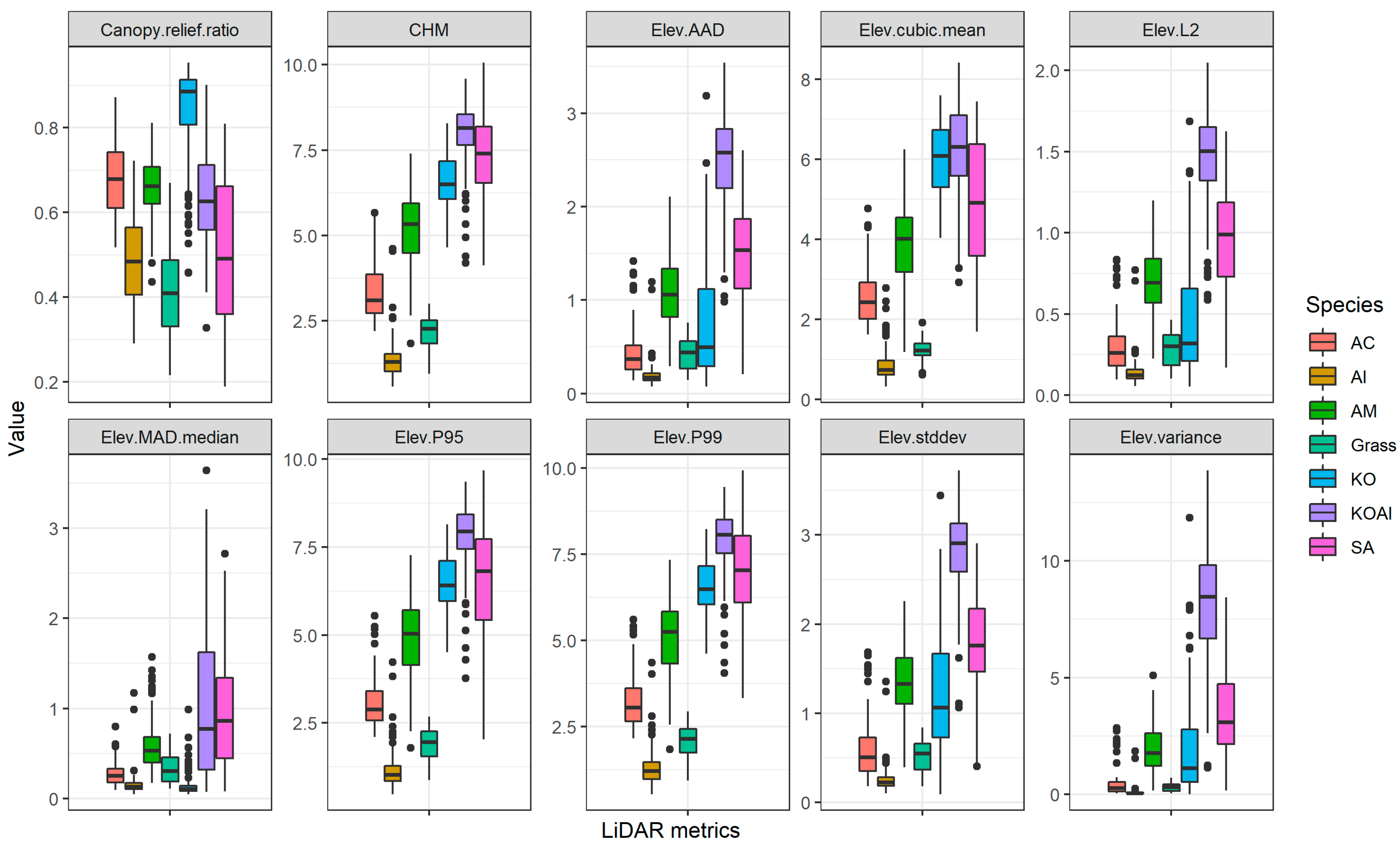
Figure 5.
Overall accuracy and Kappa changing with number of features by recursive feature elimination (RFE) basing on the Random Forest (RF).
Figure 5.
Overall accuracy and Kappa changing with number of features by recursive feature elimination (RFE) basing on the Random Forest (RF).
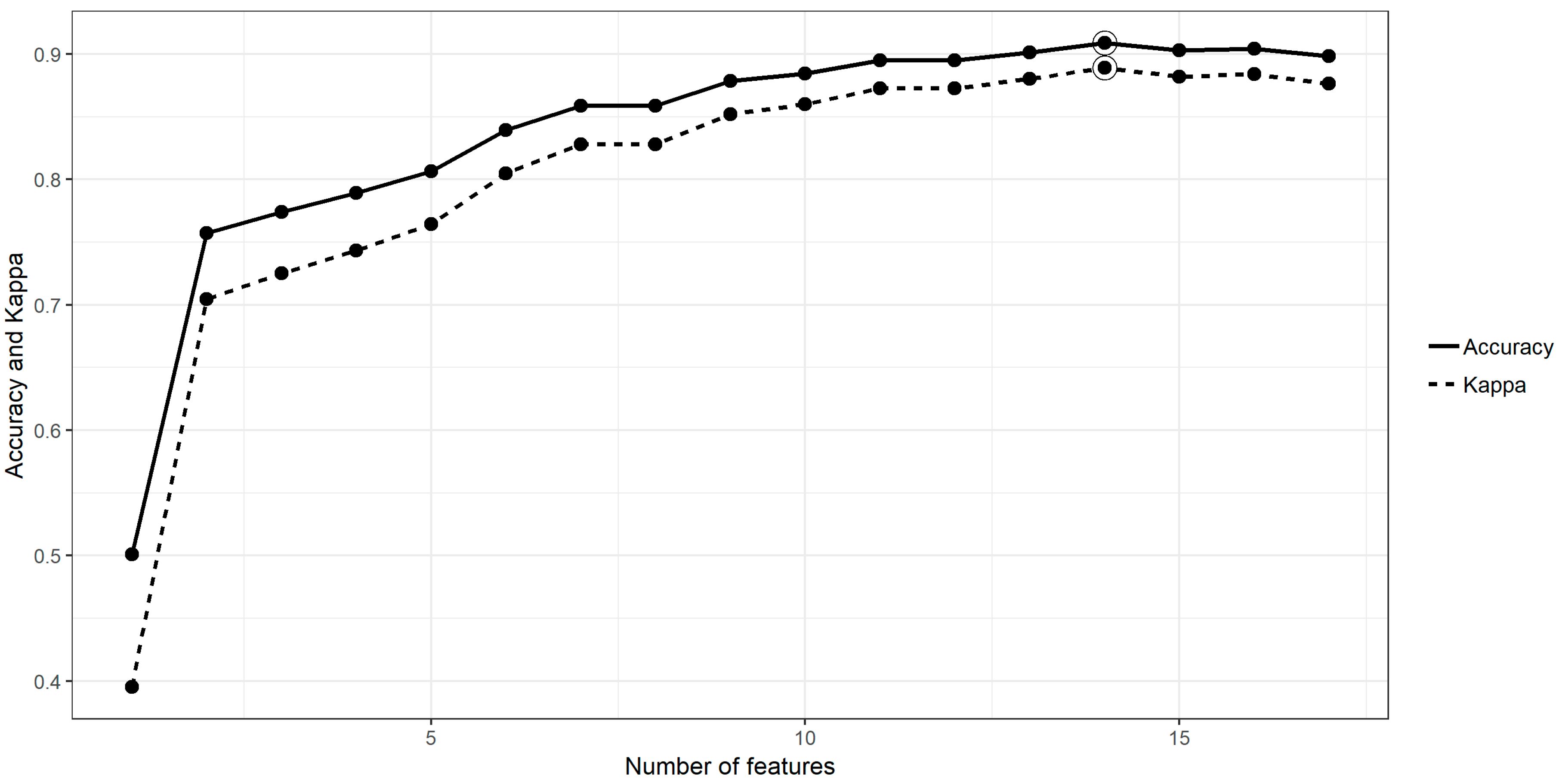
Figure 6.
(a) WV-3 multispectral image and classification image, (b) RF classification based on WV3 images, (c) RF classification based on LiDAR metrics, (d) RF classification based on Combined WV3 and LiDAR.
Figure 6.
(a) WV-3 multispectral image and classification image, (b) RF classification based on WV3 images, (c) RF classification based on LiDAR metrics, (d) RF classification based on Combined WV3 and LiDAR.
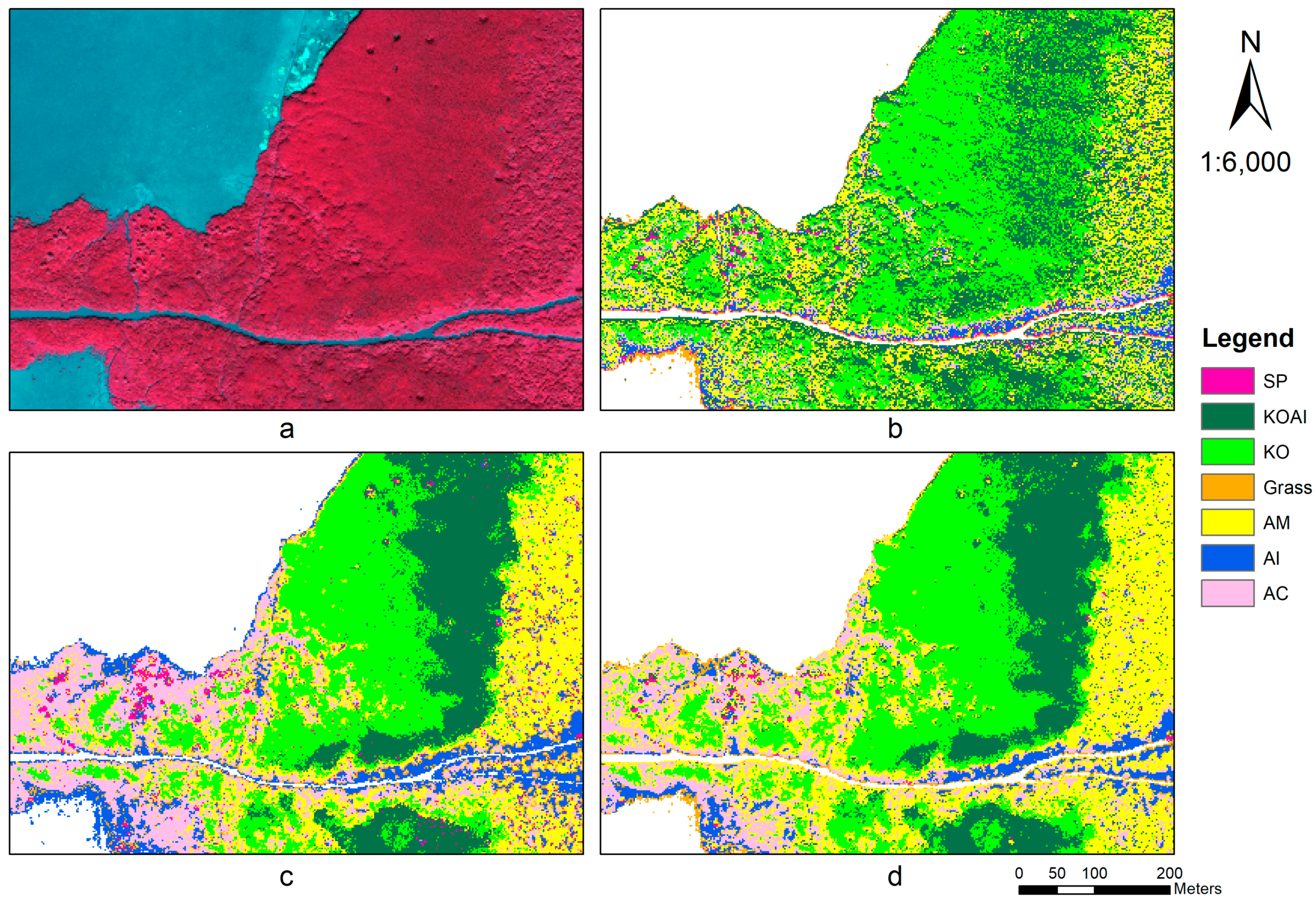
Table 1.
Specification of LiDAR (Airborne Light Detection and Ranging) system and LiDAR data.
| Specification | |
|---|---|
| Flight altitude | 155–270 m, an average of 180 m |
| Footprint diameter | 0.09 m |
| Return density | 20/m2 |
| Number of returns | 1–5 |
| Beam divergence | 0.5 mrad |
| Wavelength | Near-infrared (905 nm) |
| Scanning mechanism | Rotating mirror |
Table 2.
Vegetation types and their training and testing sample for image classification.
| Vegetation Types | Training | Testing | ||
|---|---|---|---|---|
| Samples | Pixels | Samples | Pixels | |
| Aegiceras corniculatum (AC) | 20 | 49 | 8 | 21 |
| Acanthus ilicifolius (AI) | 22 | 88 | 9 | 36 |
| Avicennia marina (AM) | 36 | 144 | 15 | 60 |
| Gramineae (Grass) | 10 | 40 | 4 | 16 |
| Kandelia obovata (KO) | 36 | 144 | 15 | 60 |
| Kandelia obovata & Acanthus ilicifolius (KOAI) | 25 | 140 | 15 | 60 |
| Sonneratia apetala (SA) | 14 | 55 | 6 | 20 |
| Total | 173 | 660 | 72 | 275 |
Table 3.
Selected features and corresponding classification accuracy.
| Data | Resolution | Selected Features (Ordering by importance) | Classification Accuracy | |||
|---|---|---|---|---|---|---|
| RF | SVM | |||||
| OA | Kappa | OA | Kappa | |||
| WV-3 MS | 2 m | B3, B6, B4, B5, B7, B2, B8 | 0.70 | 0.63 | 0.72 | 0.66 |
| WV-3 PS | 0.5 m | B3, B6, B5, B7, B4, B8, B2, B1 | 0.68 | 0.61 | 0.68 | 0.61 |
| LiDAR Metric | 2 m | CHM, Elev stddev, Elev variance, Elev P99, Elev AAD, Canopy relief ratio, Elev cubic mean, Elev L2, Elev P95, Elev MAD median | 0.79 | 0.75 | 0.79 | 0.74 |
| LiDAR Metric | 5 m | Elev variance, Elev stddev, CHM, Elev AAD, Canopy relief ratio, Elev L2, Elev skewness, (All returns above mean)/(Total first returns) * 100 | 0.78 | 0.73 | 0.78 | 0.74 |
| WV-3 + LiDAR | 2m | Elev cubic mean, CHM, Canopy relief ratio, Elev P99, Elev P95, B6, Elev stddev, Elev variance, B3, B5, B4, B2, Elev MAD median, B7 | 0.87 | 0.85 | 0.88 | 0.85 |
Table 4.
Confusion matrix for classification with WV-3 data.
| RF Classifier | ||||||||
|---|---|---|---|---|---|---|---|---|
| Reference | ||||||||
| Classified | AC | AI | AM | Grass | KO | KOAI | SA | UA |
| AC | 4 | 5 | 0 | 0 | 0 | 0 | 1 | 0.40 |
| AI | 6 | 23 | 1 | 0 | 0 | 0 | 0 | 0.77 |
| AM | 5 | 7 | 38 | 3 | 3 | 5 | 0 | 0.62 |
| Grass | 0 | 0 | 0 | 13 | 0 | 0 | 1 | 0.93 |
| KO | 6 | 0 | 4 | 0 | 50 | 8 | 0 | 0.74 |
| KOAI | 0 | 1 | 16 | 0 | 7 | 47 | 2 | 0.64 |
| SA | 0 | 0 | 1 | 0 | 0 | 0 | 18 | 0.95 |
| PA | 0.19 | 0.64 | 0.63 | 0.81 | 0.83 | 0.78 | 0.82 | |
| SVM Classifier | ||||||||
| Reference | ||||||||
| Classified | AC | AI | AM | Grass | KO | KOAI | SA | UA |
| AC | 5 | 7 | 0 | 0 | 0 | 0 | 1 | 0.38 |
| AI | 4 | 24 | 1 | 0 | 0 | 0 | 1 | 0.80 |
| AM | 4 | 4 | 37 | 1 | 3 | 7 | 0 | 0.66 |
| Grass | 0 | 0 | 0 | 15 | 0 | 0 | 0 | 1.00 |
| KO | 7 | 0 | 1 | 0 | 51 | 5 | 0 | 0.80 |
| KOAI | 1 | 1 | 20 | 0 | 6 | 48 | 2 | 0.62 |
| SA | 0 | 0 | 1 | 0 | 0 | 0 | 18 | 0.95 |
| PA | 0.24 | 0.67 | 0.62 | 0.94 | 0.85 | 0.8 | 0.82 | |
Table 5.
Confusion matrix for classification with LiDAR data.
| RF Classifier | ||||||||
|---|---|---|---|---|---|---|---|---|
| Reference | ||||||||
| Classified | AC | AI | AM | Grass | KO | KOAI | SA | UA |
| AC | 12 | 4 | 3 | 0 | 0 | 0 | 0 | 0.63 |
| AI | 1 | 26 | 0 | 6 | 0 | 0 | 0 | 0.79 |
| AM | 3 | 2 | 53 | 1 | 3 | 3 | 4 | 0.77 |
| Grass | 0 | 4 | 0 | 9 | 0 | 0 | 1 | 0.64 |
| KO | 3 | 0 | 3 | 0 | 52 | 1 | 1 | 0.87 |
| KOAI | 0 | 0 | 0 | 0 | 5 | 53 | 3 | 0.87 |
| SA | 2 | 0 | 1 | 0 | 0 | 3 | 13 | 0.68 |
| PA | 0.57 | 0.72 | 0.88 | 0.56 | 0.87 | 0.88 | 0.59 | |
| SVM Classifier | ||||||||
| Reference | ||||||||
| Classified | AC | AI | AM | Grass | KO | KOAI | SA | UA |
| AC | 9 | 3 | 0 | 1 | 0 | 0 | 1 | 0.64 |
| AI | 1 | 29 | 0 | 6 | 0 | 0 | 0 | 0.81 |
| AM | 6 | 2 | 60 | 2 | 11 | 4 | 4 | 0.67 |
| Grass | 2 | 2 | 0 | 7 | 0 | 0 | 1 | 0.58 |
| KO | 3 | 0 | 0 | 0 | 48 | 1 | 4 | 0.86 |
| KOAI | 0 | 0 | 0 | 0 | 1 | 54 | 2 | 0.95 |
| SA | 0 | 0 | 0 | 0 | 0 | 1 | 10 | 0.91 |
| PA | 0.43 | 0.81 | 1.00 | 0.44 | 0.8 | 0.9 | 0.45 | |
Table 6.
Confusion matrix for classification with combining WV-3 and LiDAR data.
| RF Classifier | ||||||||
|---|---|---|---|---|---|---|---|---|
| Reference | ||||||||
| Classified | AC | AI | AM | Grass | KO | KOAI | SA | UA |
| AC | 14 | 1 | 1 | 0 | 3 | 0 | 2 | 0.74 |
| AI | 3 | 28 | 2 | 3 | 0 | 0 | 0 | 0.93 |
| AM | 1 | 0 | 57 | 0 | 2 | 0 | 0 | 0.84 |
| Grass | 0 | 0 | 1 | 14 | 0 | 0 | 1 | 0.82 |
| KO | 0 | 0 | 3 | 0 | 55 | 2 | 0 | 0.90 |
| KOAI | 0 | 0 | 4 | 0 | 1 | 54 | 1 | 0.93 |
| SA | 1 | 1 | 0 | 0 | 0 | 2 | 18 | 0.82 |
| PA | 0.67 | 0.78 | 0.95 | 0.88 | 0.92 | 0.9 | 0.82 | |
| SVM Classifier | ||||||||
| Reference | ||||||||
| Classified | AC | AI | AM | Grass | KO | KOAI | SA | UA |
| AC | 12 | 3 | 2 | 0 | 1 | 0 | 0 | 0.67 |
| AI | 0 | 30 | 0 | 0 | 0 | 0 | 0 | 1.00 |
| AM | 4 | 3 | 57 | 1 | 1 | 4 | 1 | 0.80 |
| Grass | 0 | 0 | 0 | 14 | 0 | 0 | 0 | 1.00 |
| KO | 4 | 0 | 1 | 0 | 55 | 1 | 0 | 0.90 |
| KOAI | 0 | 0 | 0 | 0 | 3 | 55 | 2 | 0.92 |
| SA | 1 | 0 | 0 | 1 | 0 | 0 | 19 | 0.90 |
| PA | 0.57 | 0.83 | 0.95 | 0.88 | 0.92 | 0.92 | 0.86 | |
© 2019 by the authors. Licensee MDPI, Basel, Switzerland. This article is an open access article distributed under the terms and conditions of the Creative Commons Attribution (CC BY) license (http://creativecommons.org/licenses/by/4.0/).
Share and Cite
MDPI and ACS Style
Li, Q.; Wong, F.K.K.; Fung, T. Classification of Mangrove Species Using Combined WordView-3 and LiDAR Data in Mai Po Nature Reserve, Hong Kong. Remote Sens. 2019, 11, 2114. https://doi.org/10.3390/rs11182114
AMA Style
Li Q, Wong FKK, Fung T. Classification of Mangrove Species Using Combined WordView-3 and LiDAR Data in Mai Po Nature Reserve, Hong Kong. Remote Sensing. 2019; 11(18):2114. https://doi.org/10.3390/rs11182114
Chicago/Turabian StyleLi, Qiaosi, Frankie Kwan Kit Wong, and Tung Fung. 2019. "Classification of Mangrove Species Using Combined WordView-3 and LiDAR Data in Mai Po Nature Reserve, Hong Kong" Remote Sensing 11, no. 18: 2114. https://doi.org/10.3390/rs11182114
Note that from the first issue of 2016, this journal uses article numbers instead of page numbers. See further details here.