Lidar Estimates of the Anisotropy of Wind Turbulence in a Stable Atmospheric Boundary Layer

Abstract

In this paper, a method is proposed to estimate wind turbulence parameters using measurements recorded by a conically scanning coherent Doppler lidar with two different elevation angles. This methodology helps determine the anisotropy of the spatial correlation of wind velocity turbulent fluctuations. The proposed method was tested in a field experiment with a Stream Line lidar (Halo Photonics, Brockamin, Worcester, United Kingdom) under stable temperature stratification conditions in the atmospheric boundary layer. The results show that the studied anisotropy coefficient in a stable boundary layer may be up to three or larger.

1. Introduction

One of the consequences of density stratification in the atmosphere or ocean is the formation of disk-shaped density inhomogeneities due to the collapse of internal waves arising in stratified fluids [1]. In a stably stratified atmosphere, this leads to the appearance of anisotropic discoid turbulent temperature inhomogeneities. Radio occultation methods are widely used to study anisotropic turbulence in free atmosphere [2,3,4]. In accordance with previously published results [2,3], the spatial spectrum of the temperature turbulence in a stable atmosphere can be represented as the sum of an isotropic and anisotropic component, which are statistically independent. The results presented in [4] show that anisotropic turbulence begins to play the predominant role at heights above four to five kilometers, where the anisotropy coefficient (ratio of the horizontal scale to the vertical scale of the correlation of air temperature fluctuations) can exceed 30.

The anisotropy of turbulent fluctuations of temperature and wind velocity manifests in the atmospheric boundary layer (ABL) as well. To date, a number of questions regarding the anisotropy of wind turbulence remain unexplored. In particular, in the scientific literature, no data have been published on the anisotropy of wind turbulence in a stable ABL in the presence of low-level jets (LLJs). Typically, LLJs with maximum wind speed of 15–25 m/s occur at night, when stratification of the air temperature is stable, at a height of 200–700 m above ground level. The mechanism of formation of the nocturnal LLJ was described in detail by Blackadar [5]. Accounting for wind turbulence anisotropy is important in the development of ABL mathematical models used for various practical applications, such as weather forecast, wind energy, air transport safety, diffusion of atmospheric impurities, etc.

In the ABL, air flow is always turbulent. Therefore, components of the wind vector V = {V_z,V_x,V_y} (where V_z is the vertical component, and V_x and V_y are horizontal components) are random functions at time t and radius vector r = {z, x, y} in a Cartesian coordinate system centered at a point on the Earth’s surface (z is the vertical coordinate, x and y are the horizontal coordinates). Let the direction of the average horizontal wind be parallel to the axis x, and the average value of the vertical component be zero. In this case, V_x is the longitudinal component and V_y is the transverse (on the horizontal plane) component of the wind velocity vector. Average values < V_z > and < V_y > are equal to zero. Hereinafter, the angular brackets denote ensemble averaging. Denote the fluctuations of the vertical, longitudinal, and transversal components of the wind as w = V_z, u = V_x - < V_x >, and v = V_y, respectively.

Pulsed coherent Doppler lidars (PCDLs) are widely applied to investigate wind turbulence in the ABL [6,7,8,9,10,11,12,13,14,15,16,17,18,19,20,21,22,23,24,25]. Strategies to conduct measurements with a scanning PCDL to study wind turbulence have been proposed [6,15], along with methods to estimate turbulence parameters, such as momentum fluxes < wu >, < wv >, and < uv >; and variances of the vertical ${\sigma }_w^2$ = < w² >, longitudinal ${\sigma }_u^2$ = < u² >, and transversal ${\sigma }_v^2$ = < v² > components of wind velocity vector, respectively. These methods provide an estimation of the differences in magnitude of ${\sigma }_w^2$, ${\sigma }_u^2$, and ${\sigma }_v^2$ due to wind turbulence anisotropy, but do not allow estimation with respect to the spatial scales of the correlation of turbulent fluctuations of the wind velocity components, such as the integral spatial scales of longitudinal correlation $L_w={\displaystyle {\int }_0^{\infty }dr{B}_w(r,0,0)/{\sigma }_w^2}$, $L_u={\displaystyle {\int }_0^{\infty }dr{B}_u(0,r,0)/{\sigma }_u^2}$, and $L_v={\displaystyle {\int }_0^{\infty }dr{B}_v(0,0,r)/{\sigma }_{\nu }^2}$. Here, B_w(r, 0, 0) = < w(z+r, x₀, y₀)w(z, x, y) >, B_u(0, r, 0) = < u(z, x+r, y)u(z, x, y) >, and B_v(0, 0, r) = < v(z, x, y+y)v(z, x, y) > are spatial correlation functions of the vertical, longitudinal, and transversal components of the wind velocity vector, respectively.

A method was proposed for estimation of the turbulent energy dissipation rate ε and the radial velocity variance ${\overline{\sigma }}_r^2$ with measurements by a conically scanning PCDL at elevation angle ϕ [19,20]. The estimate for ${\overline{\sigma }}_r^2$ found by the method described [19,20], is a result of averaging the variances of the radial velocities measured with the lidar at all azimuth angles θ, which are set during the scan. With the assumption that the turbulence structure is described by the von Kàrmàn model [26,27], the integral scale of longitudinal correlation of the radial velocity fluctuations L_V can be calculated from the lidar estimates ε and ${\overline{\sigma }}_r^2$ by the following equation [19,20]:

$$L_V=0.698{({\overline{\sigma }}_r^2)}^{3/2}/\epsilon ,$$

(1)

The integral scale L_V is, just as ${\overline{\sigma }}_r^2$, the result of averaging over all the azimuth angles θ. Similar to ${\overline{\sigma }}_r^2$, the scale L_V at a fixed height depends on the elevation angle ϕ employed in the conical scanning due to the turbulence anisotropy, even at horizontally statistically homogeneous wind velocity fluctuations. If the scanning is conducted at the angle ϕ = tan⁻¹(1/$\sqrt{2}$) ≈ 35.3°, then the kinetic energy of turbulence E = (1/2)(${\sigma }_w^2$ + ${\sigma }_u^2$ + ${\sigma }_v^2$) can be calculated from the lidar estimates ${\overline{\sigma }}_r^2$ as E = (3/2)${\overline{\sigma }}_r^2$ [6,19,20].

In this paper, a method is proposed to estimate wind turbulence parameters, including the integral spatial scales of turbulence based on Equation (1), from lidar measurements employing conical scanning at different elevation angles. This method also allows us to determine the anisotropy of the spatial correlation of wind velocity fluctuations. The method was tested in an experiment with a Stream Line lidar (Halo Photonics, Brockamin, Worcester, United Kingdom) under stable temperature stratification conditions in the atmospheric boundary layer.

2. Lidar Method to Determine Parameters of Anisotropic Turbulence

The instantaneous radial velocity V_r, which is the projection of the wind velocity vector onto the optical axis of the probing beam, at point r = RS(θ, ϕ), can be represented in the form [14]:

$$V_r(R,\theta ,\phi )=S(\theta ,\phi )\cdot V\left(RS(\theta ,\phi )\right),$$

(2)

where R is the distance from the lidar to the point r and S(θ, ϕ) = {sin ϕ, cos ϕ cos θ, cos ϕ sin θ} is the unit vector along the optical axis. Difference V_r’ = V_r - < V_r > represents turbulent fluctuations in the radial velocity. Due to statistical inhomogeneity and anisotropy, the radial velocity variance ${\sigma }_r^2=\hspace{0.17em}<{(V_r{}^{\prime })}^2>$ is a function of both the parameters, characterizing wind turbulence, and of the distance R and the angles θ and ϕ. We assume that the wind field is statistically homogeneous in the horizontal plane. Then, the radial velocity variance ${\overline{\sigma }}_r^2(R,\phi )={(2\pi )}^{-1}{\displaystyle {\int }_0^{2\pi }d\theta \hspace{0.17em}}{\sigma }_r^2(R,\theta ,\phi )$ averaged over all azimuth angles θ (in the range from 0 to 2π) can be represented in the form [6,20]:

$${\overline{\sigma }}_r^2(h/\sin \phi ,\phi )={(\sin \phi )}^2{\sigma }_w^2(h)+{(\cos \phi )}^2{\sigma }_H^2(h),$$

(3)

where h = Rsinϕ = z is the height and ${\sigma }_H^2=({\sigma }_u^2+{\sigma }_v^2)/2$ is the wind velocity variance defined as an average of variances of the longitudinal and transversal components of the wind velocity vector in the horizontal plane. Experiments [28] showed that the variance ${\sigma }_w^2$ differs much more from the variances ${\sigma }_u^2$ and ${\sigma }_v^2$ than variances ${\sigma }_v^2$ and ${\sigma }_u^2$ differ from each other. Often, the variances ${\sigma }_v^2$ and ${\sigma }_u^2$ coincide. Therefore, for an experimental study of the anisotropy of wind turbulence, measuring only two variances: ${\sigma }_w^2$ and ${\sigma }_H^2=({\sigma }_u^2+{\sigma }_v^2)/2$ may suffice.

According to Equation (3), the variance ${\overline{\sigma }}_r^2$, besides the height h, depends on the elevation angle ϕ due to the anisotropy of turbulence (${\sigma }_w^2(h)\ne {\sigma }_H^2(h)$). To obtain estimates of the variances ${\sigma }_w^2$ and ${\sigma }_H^2$, simultaneous lidar measurements at two different elevation angles are necessary. Given two different angles ϕ = ϕ₁ and ϕ = ϕ₂ (ϕ₁ ≠ ϕ₂) in Equation (3), we obtain a system of equations for the height profiles of the variances ${\sigma }_w^2(h)$ and ${\sigma }_H^2(h)$:

$$\{\begin{array}{l}{\overline{\sigma }}_r^2(h/\sin {\phi }_1,{\phi }_1)={(\sin {\phi }_1)}^2{\sigma }_w^2(h)+{(\cos {\phi }_1)}^2{\sigma }_H^2(h)\hspace{0.17em}\\ {\overline{\sigma }}_r^2(h/\sin {\phi }_2,{\phi }_2)={(\sin {\phi }_2)}^2{\sigma }_w^2(h)+{(\cos {\phi }_2)}^2{\sigma }_H^2(h)\end{array},$$

(4)

To retrieve the vertical profile of the turbulent kinetic energy E(h) from lidar data, we take ϕ₁ = 35.3° in Equation (4) [6]. The angle ϕ₂ is taken as 60°. Then, the solution of the system of Equation (4) has the following form:

$${\sigma }_w^2(h)=\frac{1}{5}\left[8{\overline{\sigma }}_r^2\left(h/\sin {\phi }_2,{\phi }_2\right)-3{\overline{\sigma }}_r^2\left(h/\sin {\phi }_1,{\phi }_1\right)\right],$$

(5)

$${\sigma }_H^2(h)=\frac{1}{5}\left[9{\overline{\sigma }}_r^2\left(h/\sin {\phi }_1,{\phi }_1\right)-4{\overline{\sigma }}_r^2\left(h/\sin {\phi }_2,{\phi }_2\right)\right],$$

(6)

where ϕ₁ = 35.3° and ϕ₂ = 60°.

The turbulent energy dissipation rate ε is a characteristic of locally isotropic wind turbulence within the inertial subrange. In the case of statistical homogeneity of the wind field in the horizontal plane, the dissipation rate is a function of height h and does not depend on horizontal coordinates x and y. After substitution of the values of the variance ${\overline{\sigma }}_r^2\left(h/\sin {\phi }_i,{\phi }_i\right)$ and the dissipation rate ε(h) obtained from lidar measurements at different elevation angles ϕ_i (i = 1, 2) into Equation (1), the integral scales L_V(h, ϕ_i) at the angles ϕ_i are calculated. The estimation method of ${\overline{\sigma }}_r^2$ and ε from the data measured by the conically scanning PCDL is described in [20]. Employing the von Kàrmàn model in Equation (1) yields the vertical profiles of longitudinal correlation scales of fluctuations of the vertical L_w(h) and horizontal L_H(h) wind velocity, if the variance ${\overline{\sigma }}_r^2$ in Equation (1) is replaced with ${\sigma }_w^2(h)$ and ${\sigma }_H^2(h)$, respectively. Because ${\sigma }_H^2=({\sigma }_u^2+{\sigma }_v^2)/2$, we assume that the value of L_H is between values of L_u and L_v.

On obtaining scales L_V1 = L_V(h, ϕ₁) and L_V2 = L_V(h, ϕ₂) from lidar measurements at the scanning elevation angles ϕ₁ = 35.3° and ϕ₂ = 60°, and employing Equations (1), (5), and (6), the scales L_w and L_H can be respectively calculated as:

$$L_w={\left(\frac{8L_{V2}^{2/3}-3L_{V1}^{2/3}}{5}\right)}^{3/2},$$

(7)

$$L_H={\left(\frac{9L_{V1}^{2/3}-4L_{V2}^{2/3}}{5}\right)}^{3/2}.$$

(8)

To apply the described method to estimate the variances and correlation scales of fluctuations of vertical and horizontal wind velocity, measurements should be recorded simultaneously by two lidars scanning at different elevation angles. However, considering that the lidar data has to be averaged over a long period of time to obtain a statistically significant estimate of the variance of radial velocity, this method can be applied using a single lidar.

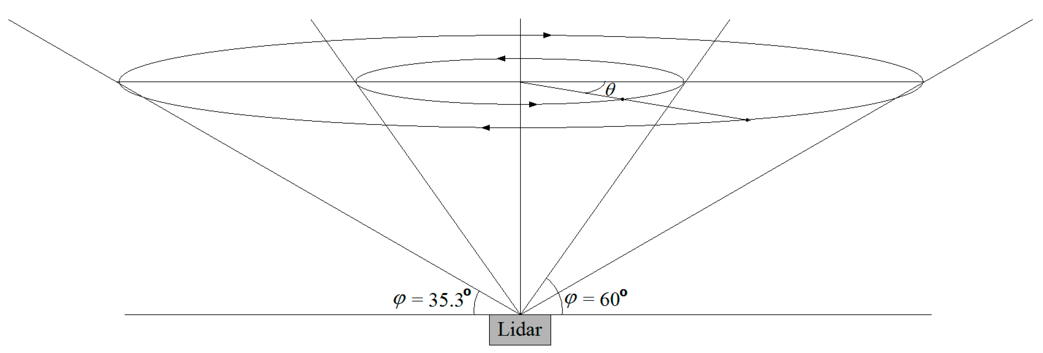
Therefore, as shown in Figure 1, the lidar probing beam conducts conical scanning about the vertical axis alternatively at the elevation angles of 35.3° (odd scan numbers) and 60° (even scan numbers).

Before the measurements were taken, elevation angle was set to ϕ = 35.3°. Then, the scanning starts with constant angular velocity ω_s = dθ/dt. During the scanning, the azimuth angle θ of the probing direction varies from 0° to 360°. After a full turn, the scanning stops and the elevation angle of 35.3° changes to 60°, which takes approximately 1 s. Then, the scanning starts in the opposite direction. The azimuth angle θ changes from 360° to 0°. At θ = 0°, the elevation angle of 60° again changes to 35.3° and the procedure repeats.

3. Experiment

The experiment was conducted on 6–24 June 2018 at the Basic Experimental Observatory (BEO) of the Institute of Atmospheric Optics SB RAS (IAO) in Tomsk, Russia (56.475448° N, 85.048115° E), employing a Stream Line PCDL (Halo Photonics, Brockamin, Worcester, United Kingdom). The experimental geometry is shown in Figure 1, which shows conical scanning with alternating elevation angle (35.3° and 60°). The duration of every scan was T_scan = 60 s. Adding the time δt ≈ 1 s needed to change the elevation angle from 35.3° to 60° and vice versa, the duration of one measurement cycle T_circl = 2(T_scan + δt) was a little bit longer than 2 min. For accumulation of raw lidar data, N_a = 7500 laser shots were used. The pulse repetition frequency was f_p = 15 kHz. Thus, the duration of measurements for every azimuth angle ∆t = N_a/f_p = 0.5 s. The azimuth resolution was ∆θ = 360°/M = 3°, where M = T_scan/∆t = 120 was the number of rays for one conical scan.

As a result of the measurements, we obtained arrays of estimates of the signal-to-noise ratio SNR (R_k, θ_m; n) and the radial velocity V_L (R_k, θ_m; n). Here, the SNR is the ratio of average heterodyne signal power to the average detector noise power in a 50 MHz bandwidth. Estimates of SNR and V_L are functions of the parameters R_k, θ_m, and n, where R_k = R₀ + k∆R is the distance from the lidar to the center of the sensing volume, k = 0,1,2,…,K−1; ∆R = 18 m is the range gate length; θ_m = m∆θ is the dependence of the azimuth angle on the ray number m = 0,1,2,…,M−1 at the elevation angle ϕ = 35.3°; θ_m = 360°−m∆θ is the azimuth angle at ϕ = 60°; n = 1,3,5,7,… is the conical scan number at the elevation angle ϕ = 35.3°; and n = 2,4,6,8,… is the conical scan number at the elevation angle ϕ = 60°. Each of the arrays SNR (R_k, θ_m; n) and V_L (R_k, θ_m; n) is divided into two sub-arrays: SNR_i (R_k, θ_m; n) and V_Li (R_k, θ_m; n) with odd (i = 1) and even (i = 2) numbers n. The subscript i = 1 corresponds to the elevation angle ϕ = 35.3°, whereas i = 2 denotes ϕ = 60°.

To increase the accuracy of SNR measurement, SNR estimates were averaged over all azimuth angles for every distance R_k and scan number n, ${\mathrm{S}\overline{\mathrm{N}}\mathrm{R}}_i(R_k,n)=M^{-1}{\displaystyle \sum _{m=0}^{M-1}{\mathrm{SNR}}_i(R_k,{\theta }_m;n)}$. Estimates of the wind velocity vector V_i(R_k, n) = {V_zi(R_k, n), V_xi(R_k, n), V_yi(R_k, n)}, where V_zi is the vertical component and V_xi and V_yi are the horizontal components, were determined from the arrays of lidar estimates of the radial velocity V_Li (R_k, θ_m; n) using the direct sine-wave fitting method [14,29]. The wind speed U_i and the wind direction angle θ_Vi were calculated from the horizontal components of the velocity vector as U_i = |V_xi + jV_yi| and θ_Vi = arg{V_xi + jV_yi }, respectively, where j is an imaginary unit.

4. Results of the Measurements

To retrieve information about turbulence from lidar data, the probability of bad (false) estimates of radial velocity has to be nearly zero [30]. That is, the SNR during the measurements should be high. For accumulation number N_a = 7500, the SNR should exceed –16 dB. Therefore, to study the anisotropy of wind turbulence in a stable ABL, we had to select data corresponding to the stable temperature stratification and SNR > –16 dB. Lidar data obtained in the 12-hour period from 20:00 on 23 July to 08:00 on 24 July met this requirement. Using the data for the average temperature of air T(h, t) measured by sonic anemometers during this time interval at heights h₁ = 3 m and h₁ = 42 m, we calculated the potential temperature derivative dT_p/dh by the equation: dT_p/dh = [T(h₂, t) − T(h₁, t) ]/(h_{2 −} h₁) + y_a, where y_a = 0.0098 °K/m is the adiabatic gradient of dry air temperature. Under the condition dT_p/dh > 0, the temperature stratification is stable; if dT_p/dh = 0, the stratification is neutral; and when dT_p/dh < 0, the stratification is unstable. Calculations show that beginning with 20:00 on 23 July to 08:00 on 24 July, the value of dT_p/dh varied in the range of 0.005 to 0.02 °K/m. Therefore, the temperature stratification of the surface atmospheric layer was stable in this period.

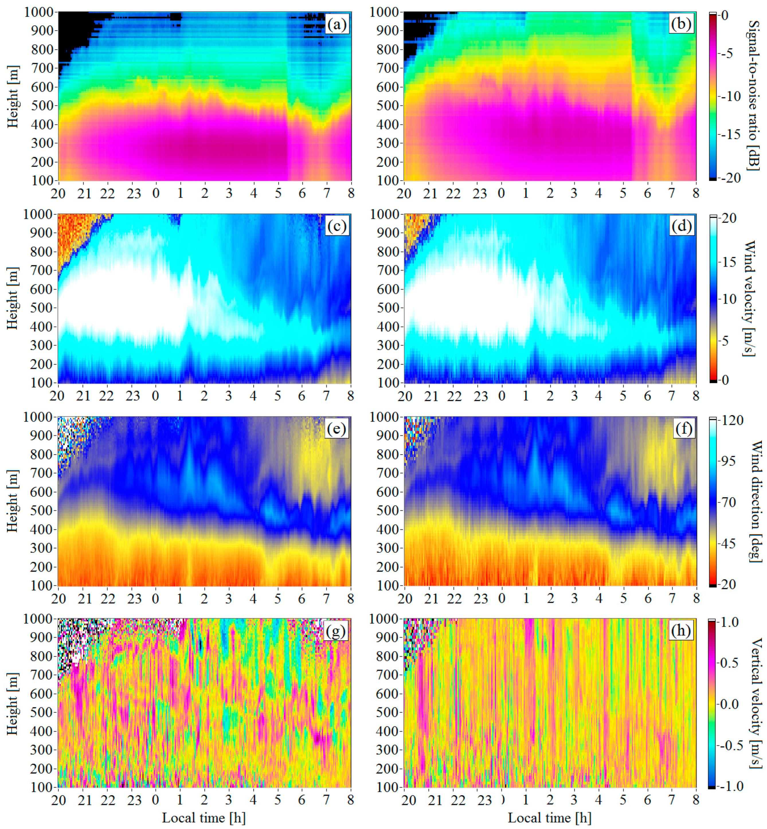
The estimates of the radial velocity with subscript k obtained from lidar measurements at different values of the elevation angles, ϕ₁ = 35.3° and ϕ₂ = 60°, correspond to different heights, h_ki = h_0i + k∆h_i, where h_0i = R₀ sin ϕ_i is the initial height and ∆h_i = ∆R sin ϕ_i is the vertical step. By sorting the obtained data in heights, two two-dimensional (2D) composite plots corresponding to the elevation angles of 35.3° and 60° were sampled for each of the following parameters: the signal-to-noise ratio ${\mathrm{S}\overline{\mathrm{N}}\mathrm{R}}_i(h_{ki},t_n)$, wind speed U_i(h_ki, t_n), wind direction angle θ_Vi(h_ki, t_n), and the vertical wind speed V_zi(h_ki, t_n). Here, t_n = t₀ + nT_circl/2 is the current time and t₀ is the measurement starting time. The obtained distributions are shown in Figure 2, which shows that the ${\mathrm{S}\overline{\mathrm{N}}\mathrm{R}}_1(h,t_n)$ for the elevation angle of 35.3° becomes much smaller than ${\mathrm{S}\overline{\mathrm{N}}\mathrm{R}}_2(h,t_n)$ for the elevation angle of 60° starting from heights at 400–500 m. This is caused by the longer distance to the probed volume at ϕ = 35.3° than at ϕ = 60° and, possibly, by the horizontal inhomogeneity of the aerosol backscatter coefficient. In the zones where ${\mathrm{S}\overline{\mathrm{N}}\mathrm{R}}_i(h_{ki},t_n)>$ –16 dB, differences in the height-time distributions of the wind speeds U₁(h_, t_n) and U₂(h_, t_n) and the wind direction angles θ_V1(h_, t_n) and θ_V2(h_, t_n) are not as significant. (Compare Figure 2c with Figure 2d and Figure 2e with Figure 2f.) These differences are mainly caused by turbulent variations in the wind field. The low-level jet (LLJ) at heights of 350–700 m is easily observed. At the LLJ center, the wind speed sometimes achieved 25 m/s. The estimates of the vertical component of the wind velocity vector at ${\mathrm{S}\overline{\mathrm{N}}\mathrm{R}}_i(h_{ki},t_n)>-16\mathrm{dB}$ do not go beyond, with one exception—the range from –1 to 1 m/s (Figure 2g–h). This agrees with the results reported by Lolli et al. [31]. Due to large-scale turbulent inhomogeneities of the wind flow and fast mesoscale processes, a significant difference was observed in estimates of vertical wind velocity V_z1(h_, t_n) and V_z2(h_, t_n).

To obtain estimates for the wind turbulence parameters, we used the measured data obtained at ${\mathrm{S}\overline{\mathrm{N}}\mathrm{R}}_i(h_{ki},t_n)>-16\mathrm{dB}$, when the probability of bad estimates of the radial velocity [32] was close to zero. According to the data in Figure 2a–b, this requirement was fulfilled for heights up to 600 m. The turbulent energy dissipation rates ε₁(h_k1, t_n) and ε₂(h_k2, t_n), radial velocity variances ${\sigma }_{r1}^2(h_{k1},t_n)$ and ${\sigma }_{r2}^2(h_{k2},t_n)$, and integral scales of turbulence L_V1(h _k1, t_n) and L_V2(h _k2, t_n) were estimated from the arrays of fluctuations of lidar estimates of the radial velocity V_Li’ using the method described thoroughly by Smalikho and Banakh [20]. Here, V_Li’(R_k, θ_m; n) = V_Li(R_k, θ_m; n) - S_i(θ_m)⋅V(R_k, n); S_i(θ_m) = {sin ϕ_i, cos ϕ_icos θ_m, cos ϕ_i sin θ_m}, i = 1,2; and i = 1 and i = 2 correspond to measurements at the elevation angles of 35.3° (odd scan numbers n) and 60° (even n), respectively. For the averaging, we used estimates of V_Li’(R_k, θ_m; n) obtained from lidar measurements for 20 scans for each elevation angle. This corresponds to 40-min time averaging.

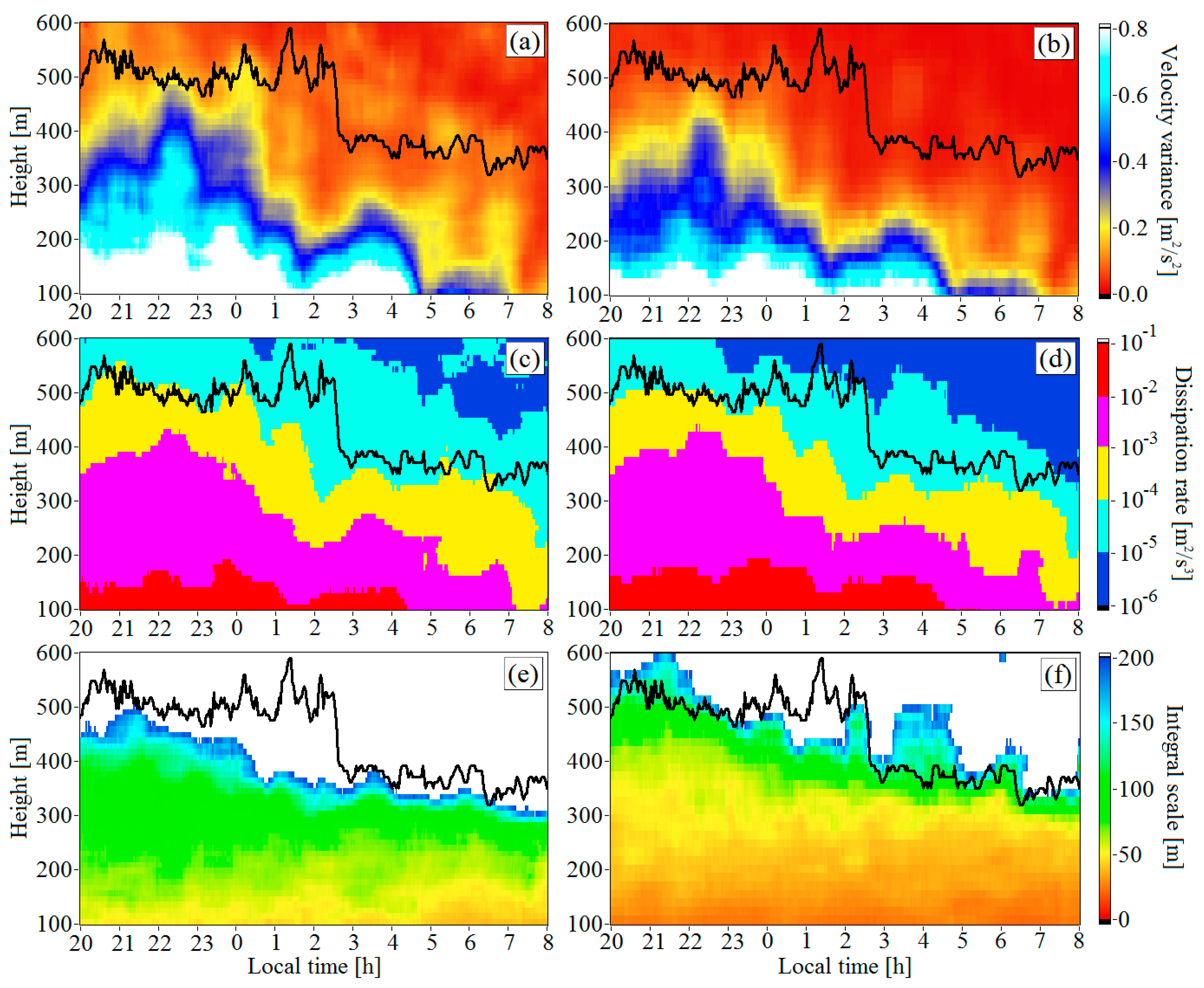
Figure 3 depicts the obtained spatiotemporal distributions of turbulence parameters ${\sigma }_{ri}^2(h_{ki},t_n)$, ε_i(h_ki, t_n), and L_Vi(h_ki, t_n). In every distribution, the black curve shows the temporal profile of the height of maximal wind speed assessed from the data in Figure 2c. This curve is a boundary between the top and bottom parts of the LLJ and can be considered as its center. The wind turbulence is very weak in the top part of the LLJ; in particular, the turbulent energy dissipation rate does not exceed 10^–4 m²/s³, and the variance of radial velocity ${\sigma }_{r2}^2(h_{k2},t_n)$ at the elevation angle of 60° is below 0.08 m²/s².

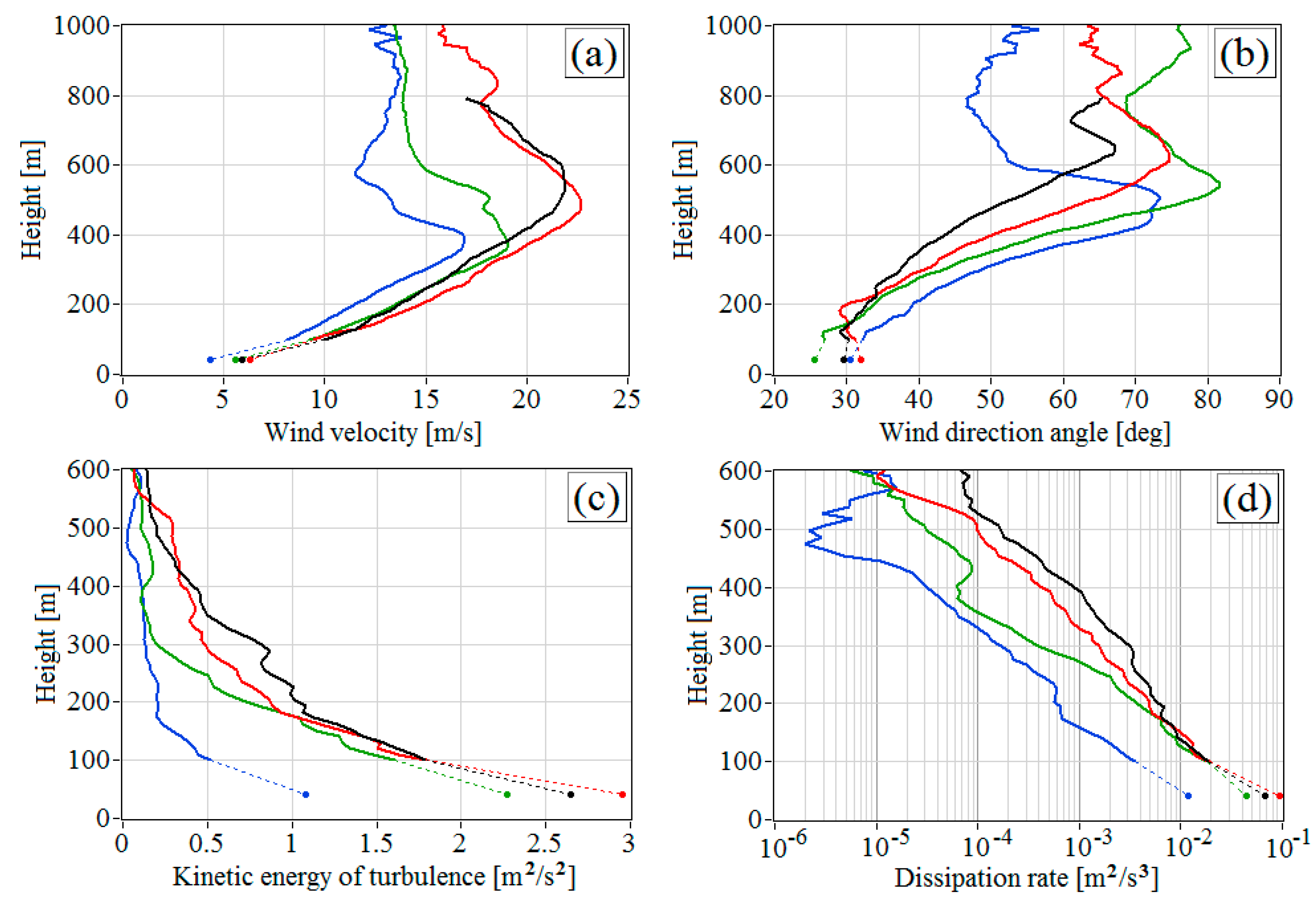
Assuming horizontal statistical homogeneity of the wind, the kinetic energy of turbulence was calculated as $E(h_{k1},t_n)=(3/2){\sigma }_{r1}^2(h_{k1},t_n)$ from the data for the variance of radial velocity ${\sigma }_{r1}^2(h_{k1},t_n)$ obtained from measurements at the elevation angle of 35.3°. Combining calculated E(h_k1, t_n) and data of Figure 2c,e, and Figure 3a,c, we drew vertical profiles of the wind speed and direction, kinetic energy of turbulence, and its dissipation rate in Figure 4. The turbulence was strong on 23 July in the bottom part of the LLJ at heights 200–400 m at wind speeds exceeding 15 m/s. The kinetic energy E ranged from 1.0 to 0.5 m²/s², and the dissipation rate varied within 7 10^–3–10^–3 m²/s³. We calculated the errors of estimation of the kinetic energy E and the dissipation rate ε using the technique described in [30]. According to our calculations, the relative error of the kinetic energy estimates was 7%–10% in the bottom part of the LLJ, whereas the accuracy of the dissipation rate estimates was 6%–8%.

In this experiment, the minimum height for retrieving vertical profiles of velocity from lidar measurements with acceptable accuracy was 100 m. The maximum height at which measurements were recorded with sonic anemometers was 42 m (a sonic anemometer was installed on top of the mast, located 150 m from the lidar). In Figure 4, in addition to lidar data, we depict the results of measurements with the sonic anemometer at a height of 42 m. Sonic anemometer measurement data show that, despite the conditions of stable temperature stratification, in the surface layer of the atmosphere (layer thickness of about 100 m in height above the ground), wind turbulence was quite strong.

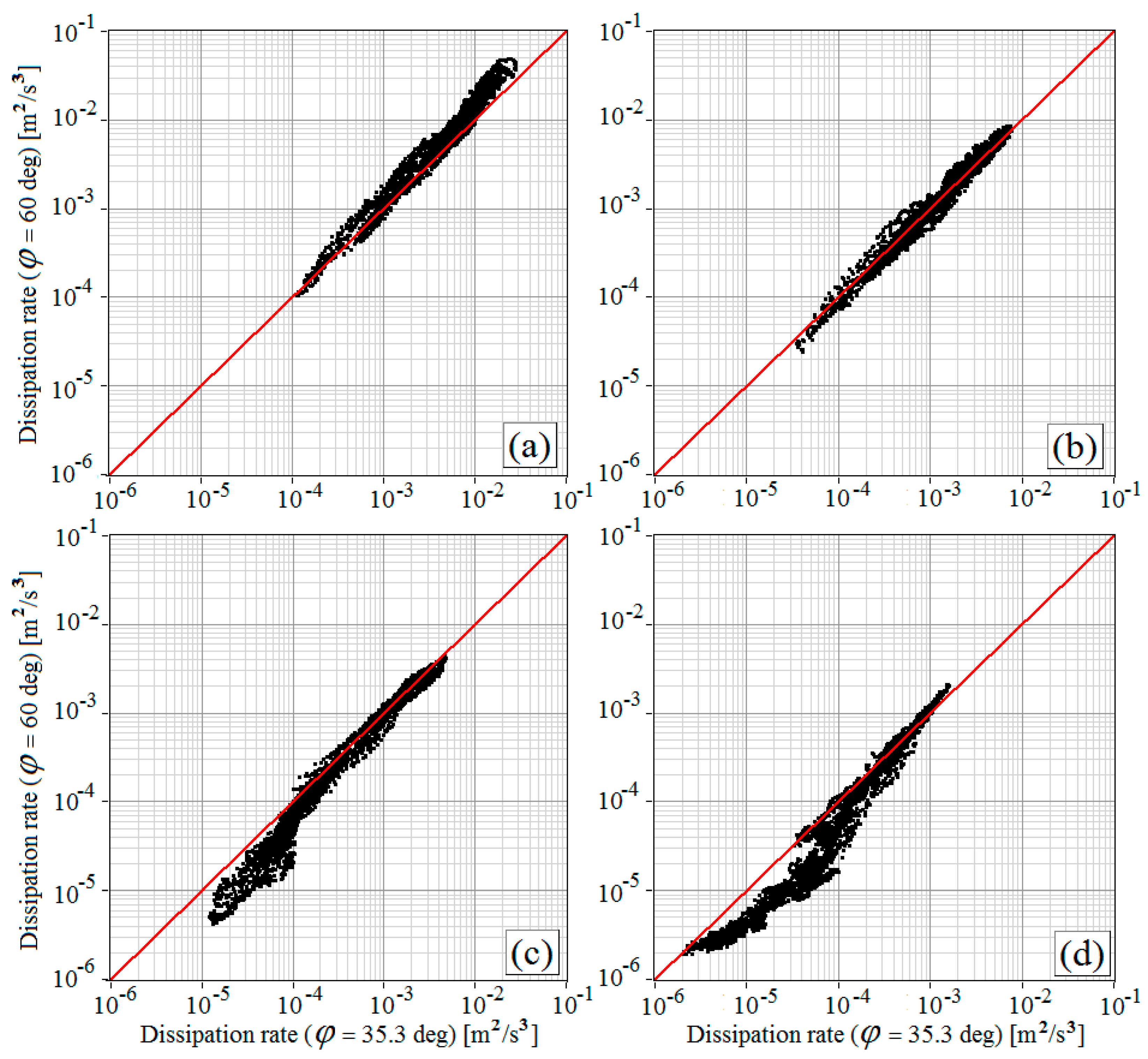
The turbulent energy dissipation rate is a characteristic of the locally isotropic field of wind velocities. Assuming that the wind velocity field is statistically homogeneous in the horizontal plane, the lidar estimates of the dissipation rates ε₁(h_, t_n) and ε₂(h_, t_n) obtained for the same height h, but for different elevation angles (35.5° and 60°), should fully coincide on average. To verify this, we used the data in Figure 3c–d and their vertical interpolation with a step of 10 m, starting from 100 m and ending at a height of 500 m.

Figure 5 depicts the results of the comparison of the lidar estimates of the dissipation rate ε₁(h_, t_n) and ε₂(h_, t_n) in four vertical layers: (1) 100–200, (2) 200–300, (3) 300–400, and (4) 400–500 m. The analysis of these results showed that, on average, ε₁ is 20% less than ε₂ in the first layer, ε₁ and ε₂ practically coincide in the second layer, and ε₁ exceeds ε₂ 1.5 and 2 times in the third and fourth layers, respectively. The reason for the small discrepancy in dissipation rate estimates in the lowest layers is unclear. On average, at heights from 170 m to 320 m, the absolute value of the discrepancy between of the dissipation rate estimates [2(ε₁ – ε₂)/(ε₁ + ε₂)]×100% does not exceed 10%. This indicates the horizontal statistical homogeneity of the wind velocity field at these heights. The significant discrepancy of the dissipation rate estimates from lidar measurements at the elevation angles of 35.3° and 60° in the upper layers may originate from horizontal mesoscale inhomogeneities in the wind field caused, for example, by internal atmospheric waves being stronger against the weakly turbulent background.

Accessible experimental data (see, for example, [28]) indicate that in the atmospheric boundary layer, the variance of horizontal wind velocity ${\sigma }_H^2(h)$ exceeds the variance of the vertical component ${\sigma }_w^2(h)$, and the correlation scale of the fluctuations of the horizontal velocity L_u(h) is larger than the correlation scale of fluctuations of the vertical velocity L_W(h) due to anisotropy of wind turbulence. Since ${\sigma }_H^2>{\sigma }_w^2$, according to Equation (4), we expect that the variance ${\overline{\sigma }}_r^2\left(h/\sin {\phi }_1,{\phi }_1\right)$ exceeds ${\overline{\sigma }}_r^2\left(h/\sin {\phi }_2,{\phi }_2\right)$ in our experiment at the elevation angles ϕ₁ = 35.3° < ϕ₂ = 60°.

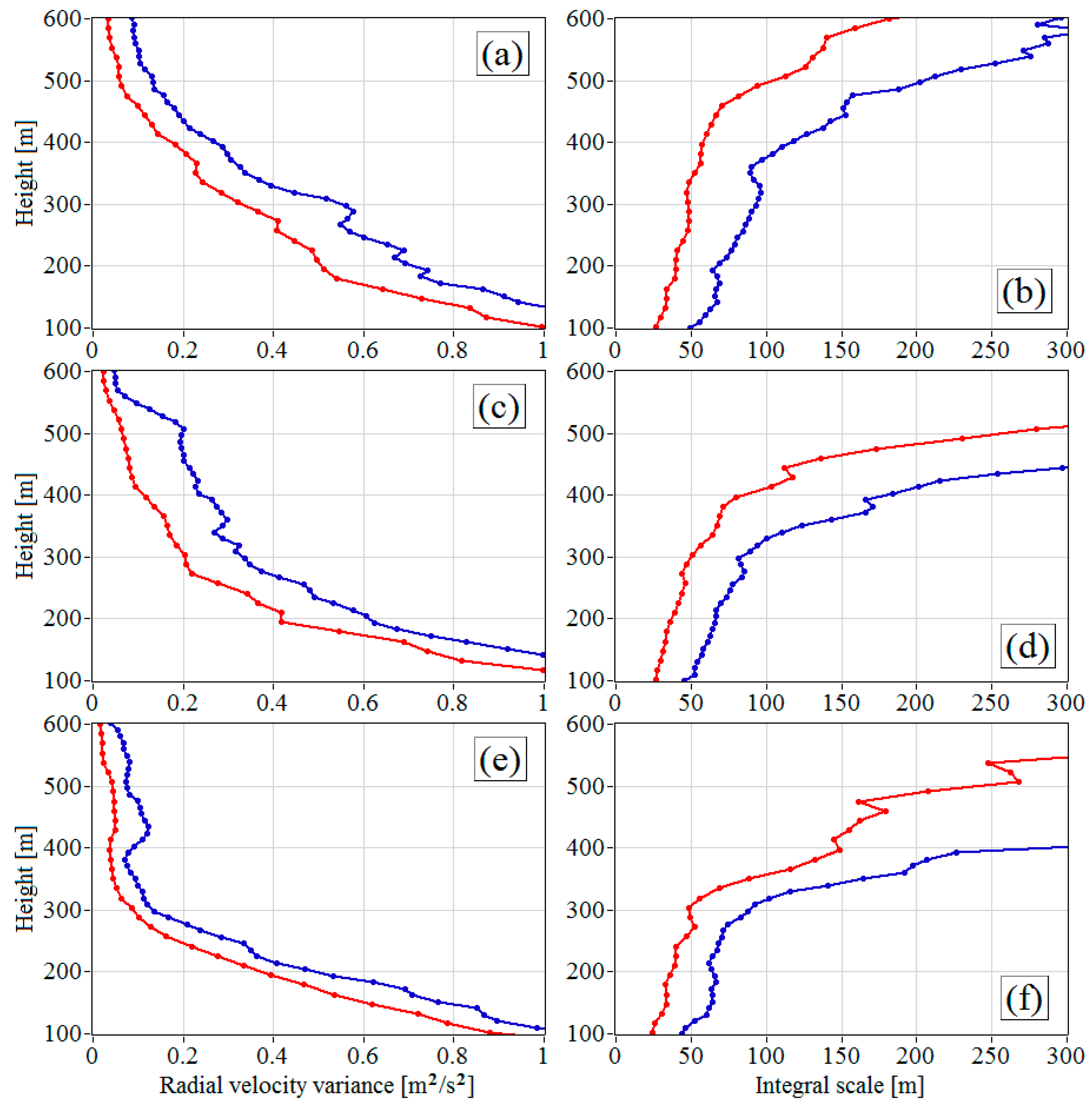
Figure 6 shows the vertical profiles of the variances ${\overline{\sigma }}_{r1}^2(h_{k1})={\overline{\sigma }}_r^2\left(R_k,{\phi }_1\right)$ and ${\overline{\sigma }}_{r2}^2(h_{k2})={\overline{\sigma }}_r^2\left(R_k,{\phi }_2\right)$, and integral correlation scales L_V1(h_k1) = L_V(R_k, ϕ₁) and L_V2(h_k2) = L_V(R_k, ϕ₂) of the radial velocity fluctuations, as retrieved from the lidar measurements at elevation angles ϕ = ϕ₁ = 35.3° and ϕ = ϕ₂ = 60°, respectively. At the same height h, the variance satisfies ${\overline{\sigma }}_{r1}^2>{\overline{\sigma }}_{r2}^2$ (Figure 6a,c,e). The integral scales L_Vi were calculated, according to Equation (1), as:

$$L_{Vi}=0.698{({\overline{\sigma }}_{ri}^2)}^{3/2}/{\epsilon }_i$$

(9)

From the analysis of the results of estimation of the turbulent energy dissipation rate ε_i shown in Figure 5, ε₁ ≈ ε₂ at heights of 100–320 m and ε₁ > ε₂ at heights of 320–500 m. This means that L_V1 obtained by Equation (9) in the 320–500 m layer is underestimated, whereas the L_V2 in this layer is overestimated. In spite of that, the inequality L_V1(h) > L_V2(h) holds at all heights, due to the anisotropy of turbulence (Figure 6b,d,f).

The data in Figure 3a–b show that the ratio of the radial velocity variances $\mu ={\sigma }_{r1}^2/{\sigma }_{r2}^2$ averaged employing all estimates in the 100–300 m layer is equal to 1.4. Thus, on average, the ratio of the integral scales is L_V1/L_V2 = μ^3/2 = 1.7. Approximately the same result L_V1/L_V2 ≈ 1.8 was obtained from direct averaging of the ratios of the integral scales in this layer based on the data in Figure 3e–f. Thus, due to the anisotropy of turbulence, the variance of the radial velocity at the elevation angle of 35.3° is 1.4 times larger than that at 60°, whereas the integral scale of turbulence at the elevation angle of 35.3° exceeds the integral scale at the elevation angle of 60° by 1.7 times.

Assuming that the wind field is horizontally statistically homogeneous in the 100–300 m layer, applying ${\sigma }_{ri}^2={\sigma }_w^2{\sin }^2{\phi }_i+{\sigma }_H^2{\cos }^2{\phi }_i$ (Equation (3) [20]), where ϕ₁ = 35.3° and ϕ₂ = 60°, we find:

$${\nu }_{\sigma }=\frac{{\sigma }_H^2}{{\sigma }_w^2}=\frac{9\mu -4}{8-3\mu }$$

(10)

for the ratio of the average between the variances of the longitudinal and transversal components of the wind vector ${\sigma }_H^2=({\sigma }_u^2+{\sigma }_v^2)/2$ to the variance of vertical component ${\sigma }_w^2$. Substituting μ = 1.4 into Equation (10) yields that the variance ${\sigma }_H^2$ is 2.26 times larger than the variance ${\sigma }_w^2$. On the assumption that the spatial structure of the wind turbulence is described by the von Kàrmàn model (Equation (1)), we obtain ${\nu }_L=L_H/L_w={({\sigma }_H^2/{\sigma }_w^2)}^{3/2}$ for the ratio of integral longitudinal correlation scales of fluctuations in the horizontal L_H and vertical L_w components of the wind velocity vector. Substituting ${\sigma }_H^2/{\sigma }_w^2$ = 2.26 into this formula yields that the correlation scale of fluctuations of the horizontal wind component L_H is 3.4 times larger than that of fluctuations of the vertical component L_w. The obtained estimates of the anisotropy coefficient of wind turbulence parameters do not contradict the known experimental data [28].

Using the data (three components of the wind vector) measured with a sonic anemometer at a height of 42 m (Figure 4), we obtained the variances ${\sigma }_H^2(t)$ and ${\sigma }_w^2(t)$versus time t for the period under consideration from 20:00 on 23 July to 08:00 on 24 July 2018. Each variance estimate was derived from 30-minute measurement data. The anisotropy coefficient ${\sigma }_H^2/{\sigma }_w^2$ averaged over all the measurement period was approximately 2, which is only 13% less than the lidar estimate (v_σ = 2.26) for heights of 100–300 m.

As follows from Figure 3e–f and Figure 6b,d,f, the lidar estimate of the integral scale $L_{Vi}$ increases with height and takes overstated values at heights above 450 m at the central and upper parts of the LLJ. In Figure 3e–f, the zones where the estimates of the integral scale of turbulence L_Vi(h_ki,t_n) exceed 200 m are shown in white. To find the reason for this error, by analogy with Banakh and Smalikho. [25], we studied fluctuations in the lidar estimates of the radial velocity ${V^{\prime }}_{Li}(R_k,{\theta }_m;n)$. As a result, we found that inhomogeneities in the wind flow with scales comparable to the base radius of the scan cone occur above 300 m. This effect is mostly pronounced at the central part of the LLJ and especially in the zones where the wind direction changes strongly with height (Figure 2e–f and Figure 4b). It is possible that mesoscale processes occur here, like internal atmospheric waves arising under stable temperature stratification conditions and a strong change in the wind velocity with height.

For a more accurate estimation of the scales L_H and L_w in the upper part of the LLJ, we used the following approach. Consider the 100–300 m layer, where the contribution of mesoscale processes to wind variations is negligibly small in comparison with wind turbulence, and the conditions of horizontally statistically homogeneous turbulence are fulfilled (ε₁ ≈ ε₂, Figure 5). In this layer, as depicted in Figure 6b,d,f, on average, the integral scales L_V1 and L_V2 increase linearly with height and have realistic values. Thus, at a height 100 m, on average, L_V1 = 45 m and L_V2 = 26 m, whereas at 300 m L_V1 = 93 m and L_V2 = 51 m. Assuming that in the 300–500 m layer, the characteristic of the change in the integral scale L_Vi with height does not considerably differ from that observed in the lower layer, we linearly extrapolated the scales in the 100–300 m layer to higher layers. As a result, we found that at h = 500 m, the integral scales are L_V1 = 136 m and L_V2 = 80 m. These values of the turbulent scales L_Vi for the central part of the LLJ do not contradict the published experimental data [25]. According to Equations (7) and (8), at the central part of the LLJ at a height of 500 m with L_V1= 136 m and L_V2 = 80 m, the horizontal L_H and vertical L_w scales of longitudinal correlation of wind velocity are approximately 183 m and 54 m, respectively.

5. Conclusions

In this paper, we proposed a method for the determination of wind turbulence parameters from PCDL measurements employing conical scanning at two different elevation angles. This method assesses the anisotropy of the spatial correlation of the wind velocity turbulent fluctuations. The method was successfully tested in an atmospheric experiment with a Stream Line lidar (Halo Photonics, Brockamin, Worcester, United Kingdom) under conditions of stable temperature stratification of the atmospheric boundary layer.

We found that the variance in radial velocity measured at an elevation angle of 35.3° always exceeds the variance in radial velocity measured at an elevation angle of 60°. The averaged ratio of these variances is 1.4. Assuming that the turbulence spatial spectrum is described by the von Kàrmàn model, we obtained that the ratio of the integral scales of fluctuations of the radial velocity measured with scanning at angles of 35.3° and 60° is approximately equal to 1.7. It follows from the obtained estimates of turbulence anisotropy that the variance of the horizontal velocity exceeds the variance of the vertical wind velocity 2.26 times. Correspondingly, the ratio of the integral correlation scale of fluctuations of the horizontal wind velocity to that of the vertical velocity is approximately 3.4. At the central part of the LLJ observed during the experiment, at heights of 400–500 m, the integral scales of fluctuations of the horizontal and vertical wind velocity components are, on average, 183 and 54 m, respectively.

References

- Barenblatt, G.I.; Monin, A.S. On a possible mechanism of the phenomenon of discoid formations in the atmosphere. Dokl. Akad. Nauk SSSR 1979, 246, 834–837. (In Russian) [Google Scholar]
- Gurvich, A.S.; Brekhovskikh, V.L. Study of the Turbulence and Inner Waves in the Stratosphere Based on the Observations of Stellar Scintillations from Space: A Model of Scintillation Spectra. Waves Random Media 2001, 11, 163–181. [Google Scholar] [CrossRef]
- Gurvich, A.S.; Kan, V. Structure of air density irregularities in the stratosphere from spacecraft observations of stellar scintillation: 1. Three-dimensional spectrum model and recovery of its parameters. 2. Characteristic scales, structure characteristics, and kinetic energy dissipation. Izv. Atmos. Ocean. Phys. 2003, 39, 300–321. [Google Scholar]
- Kan, V.; Gorbunov, M.E.; Sofieva, V.F. Fluctuations of radio occultation signals in sounding the Earth’s atmosphere. Atmos. Meas. Tech. 2018, 11, 663–680. [Google Scholar] [CrossRef]
- Blackadar, A.K. Boundary layer wind maxima and their significance for the growth of nocturnal inversions. Bull. Am. Meteorol. Soc. 1957, 38, 283–290. [Google Scholar] [CrossRef]
- Eberhard, W.L.; Cupp, R.E.; Healy, K.R. Doppler lidar measurement of profiles of turbulence and momentum flux. J. Atmos. Ocean. Technol. 1989, 6, 809–819. [Google Scholar] [CrossRef]
- Frehlich, R.G.; Hannon, S.M.; Henderson, S.W. Coherent Doppler lidar measurements of wind field statistics. Bound.-Layer Meteorol. 1998, 86, 223–256. [Google Scholar] [CrossRef]
- Smalikho, I.N.; Köpp, F.; Rahm, S. Measurement of atmospheric turbulence by 2-μm Doppler lidar. J. Atmos. Ocean. Technol. 2005, 22, 11, 1733–1747. [Google Scholar] [CrossRef]
- Frehlich, R.G.; Meillier, Y.; Jensen, M.L.; Balsley, B.; Sharman, R. Measurements of boundary layer profiles in urban environment. J. Appl. Meteorol. Climatol. 2006, 45, 821–837. [Google Scholar] [CrossRef]
- Banta, R.M.; Pichugina, Y.L.; Brewer, W.A. Turbulent velocity-variance profiles in the stable boundary layer generated by a nocturnal low-level jet. J. Atmos. Sci. 2006, 63, 2700–2719. [Google Scholar] [CrossRef]
- Banakh, V.A.; Smalikho, I.N.; Pichugina, E.L.; Brewer, W.A. Representativeness of Measurements of the Dissipation Rate of Turbulence Energy by Scanning Doppler Lidar. Atmos. Ocean. Opt. 2010, 23, 48–54. [Google Scholar] [CrossRef]
- O’Connor, E.J.; Illingworth, A.J.; Brooks, I.M.; Westbrook, C.D.; Hogan, R.J.; Davies, F.; Brooks, B.J. A method for estimating the kinetic energy dissipation rate from a vertically pointing Doppler lidar, and independent evaluation from balloon-borne in situ measurements. J. Atmos. Ocean. Technol. 2010, 27, 1652–1664. [Google Scholar] [CrossRef]
- Sathe, A.; Mann, J. A review of turbulence measurements using ground-based wind lidars. Atmos. Meas. Tech. 2013, 6, 3147–3167. [Google Scholar] [CrossRef] [Green Version]
- Banakh, V.A.; Smalikho, I.N. Coherent Doppler Wind Lidars in a Turbulent Atmosphere; Artech House Publishers: Boston, MA, USA; London, UK, 2013; ISBN 978-1-60807-667-3. [Google Scholar]
- Sathe, A.; Mann, J.; Vasiljevic, N.; Lea, G. A six-beam method to measure turbulence statistics using ground-based wind lidars. Atmos. Meas. Tech. 2014, 7, 10327–10359. [Google Scholar] [CrossRef]
- Fuertes, F.C.; Iungo, G.V.; Porté-Agel, F. 3D turbulence measurements using three synchronous wind lidars: Validation against sonic anemometry. J. Atmos. Ocean. Technol. 2014, 31, 1549–1556. [Google Scholar] [CrossRef]
- Smalikho, I.N.; Banakh, V.A.; Falits, A.V.; Rudi, Y.A. Determination of the turbulent energy dissipation rate from data measured by a “Stream Line” lidar in the atmospheric surface layer. Opt. Atmos. Okeana 2015, 28, 901–905. (In Russian) [Google Scholar] [CrossRef]
- Newman, J.F.; Klein, P.M.; Wharton, S.; Sathe, A.; Bonin, T.A.; Chilson, P.B.; Muschinski, A. Evaluation of three lidar scanning strategies for turbulence measurements. Atmos Meas. Tech. 2016, 9, 1993–2013. [Google Scholar] [CrossRef] [Green Version]
- Smalikho, I.N.; Banakh, V.A.; Falits, A.V. Lidar measurements of wind turbulence parameters in the atmospheric boundary layer. Opt. Atmos. Okeana 2017, 30, 342–349. (In Russian) [Google Scholar] [CrossRef]
- Smalikho, I.N.; Banakh, V.A. Measurements of wind turbulence parameters by a conically scanning coherent Doppler lidar in the atmospheric boundar layer. Atmos. Meas. Tech. 2017, 10, 4191–4208. [Google Scholar] [CrossRef]
- Bonin, T.A.; Choukulkar, A.; Brewer, W.A.; Sandberg, S.P.; Weickmann, A.M.; Pichugina, Y.; Banta, R.M.; Oncley, S.P.; Wolfe, D.E. Evaluation of Turbulence Measurement Techniques from a Single Doppler Lidar. Atmos. Meas. Tech. 2017, 10, 3021–3039. [Google Scholar] [CrossRef]
- Newman, J.F.; Clifton, A. An error reduction algorithm to improve lidar turbulence estimates for wind energy. Wind Energy Sci. 2017, 2, 77–95. [Google Scholar] [CrossRef] [Green Version]
- Bodini, N.; Lundquist, J.K.; Newsom, R.K. Estimation of turbulence dissipation rate and its variability from sonic anemometer and wind Doppler lidar during the XPIA field campaign. Atmos. Meas. Tech. 2018, 11, 4291–4308. [Google Scholar] [CrossRef] [Green Version]
- Stephan, A.; Wildmann, N.; Smalikho, I.N. Measurements of wind turbulence parameters by a Windcube 200s lidar in the atmospheric boundary layer. Opt. Atmos. Okeana 2018, 31, 815–820. (In Russian) [Google Scholar] [CrossRef]
- Banakh, V.A.; Smalikho, I.N. Lidar studies of wind turbulence in the stable atmospheric boundary layer. Remote Sens. 2018, 10, 1219. [Google Scholar] [CrossRef]
- Von Kàrmàn, T. Progress in the statistical theory of turbulence. Proc. Natl. Acad. Sci. USA 1948, 34, 530–539. [Google Scholar] [CrossRef] [PubMed]
- Smalikho, I.N.; Banakh, V.A. Accuracy of Estimation of the Turbulent Energy Dissipation Rate from Wind Measurements with a Conically Scanning Pulsed Coherent Doppler Lidar. Part I. Algorithm of Data Processing. Atmos. Ocean. Opt. 2013, 26, 404–410. [Google Scholar] [CrossRef]
- Byzova, N.L.; Ivanov, V.N.; Garger, E.K. Turbulence in Atmospheric Boundary Layer; Gidrometeoizdat: Leningrad, Russia, 1989; p. 265, (In Russian). ISBN 5-286-00151-3. [Google Scholar]
- Smalikho, I. Techniques of wind vector estimation from data measured with a scanning coherent Doppler lidar. J. Atmos. Ocean. Technol. 2003, 20, 276–291. [Google Scholar] [CrossRef]
- Banakh, V.A.; Smalikho, I.N.; Falits, V.A. Estimation of the turbulence energy dissipation rate in the atmospheric boundary layer from measurements of the radial wind velocity by micropulse coherent Doppler lidar. Opt. Express 2017, 25, 22679–22692. [Google Scholar] [CrossRef] [PubMed]
- Lolli, S.; Delaval, A.; Loth, C.; Garnier, A.; Flamant, P.H. 0.355-micrometer direct detection wind lidar under testing during a field campaign in consideration of ESA’s ADM-Aeolus mission. Atmos. Meas. Tech. 2013, 6, 3349–3358. [Google Scholar] [CrossRef]
- Frehlich, R.G.; Yadlowsky, M.J. Performance of mean-frequency estimators for Doppler radar and lidar. J. Atmos. Ocean. Technol. 1994, 11, 1217–1230. [Google Scholar] [CrossRef]
Figure 1.
Geometry of lidar measurement employing alternate conical scanning around the vertical axis at the elevation angles (ϕ) of 35.3° and 60°.
Figure 2.
Height and time distribution of the (a,b) signal-to-noise ratio (SNR), (c,d) horizontal wind velocity, (e,f) wind direction angle, and (g,h) the vertical component of the wind velocity vector obtained from lidar measurements at the Basic Experimental Observatory of the Institute of Atmospheric Optics, Siberian Branch of the Russian Academy of Sciences (Tomsk, Russia) on 23–24 July 2018 employing conical scanning at elevation angles of (a,c,e,g) 35.3° and (b,d,f,h) 60°.
Figure 3.
Height and time distributions of the (a,b) radial velocity variance, (c,d) turbulent energy dissipation rate, and (e,f) integral scale of turbulence obtained from lidar measurements at the Basic Experimental Observatory of the IAO on 23–24 July 2018 employing conical scanning at elevation angles of (a,c,e) 35.3° and (b,d,f) 60°. Black curves show the time profile of the height of maximal wind speed in the vertical distribution of the speed within low-level jet (LLJ).
Figure 4.
Vertical profiles of (a) wind velocity, (b) wind direction angle, (c) kinetic energy of turbulence, and (d) turbulent energy dissipation rate retrieved from measurements by the lidar employing conical scanning at the elevation angle of 35.3° at 21:00 local time (LT) on 23 July (black curves) and 00:00 (red curves), 03:00 (green curves), and 06:00 LT (blue curves) on 24 July 2018. The profiles of wind velocity and wind direction angle were retrieved from the data of one scan (measurement duration of 1 min), whereas the profiles of wind turbulence parameters were retrieved from the data of 20 scans. The circles indicate the results of measurements with a sonic anemometer at a height of 42 m. The dotted lines “stitch” the corresponding data, which is measured using a sonic anemometer and lidar.
Figure 5.
Comparison of estimates of the turbulent energy dissipation rate (black dots) obtained from measurements by the lidar at elevation angles of 35.3° and 60° from 20:00 LT on 23 July to 08:00 LT on 24 July 2018 in the vertical layers of (a) 100–200, (b) 200–300, (c) 300–400, and (d) 400–500 m. Each estimate of the dissipation rate was obtained from data of 20 conical scans.
Figure 6.
Vertical profiles of the (a,c,e) radial velocity variance and (b,d,f) integral scale of turbulence retrieved from measurements by the lidar at the elevation angles of 35.3° (blue curves) and 60° (red curves) at (a,b) 21:00 LT on 23 July, and (c,d) 00:00 and (e,f) 03:00 LT on 24 July 2018.
© 2019 by the authors. Licensee MDPI, Basel, Switzerland. This article is an open access article distributed under the terms and conditions of the Creative Commons Attribution (CC BY) license (http://creativecommons.org/licenses/by/4.0/).
Share and Cite
MDPI and ACS Style
Banakh, V.A.; Smalikho, I.N. Lidar Estimates of the Anisotropy of Wind Turbulence in a Stable Atmospheric Boundary Layer. Remote Sens. 2019, 11, 2115. https://doi.org/10.3390/rs11182115
AMA Style
Banakh VA, Smalikho IN. Lidar Estimates of the Anisotropy of Wind Turbulence in a Stable Atmospheric Boundary Layer. Remote Sensing. 2019; 11(18):2115. https://doi.org/10.3390/rs11182115
Chicago/Turabian StyleBanakh, Viktor A., and Igor N. Smalikho. 2019. "Lidar Estimates of the Anisotropy of Wind Turbulence in a Stable Atmospheric Boundary Layer" Remote Sensing 11, no. 18: 2115. https://doi.org/10.3390/rs11182115
Note that from the first issue of 2016, this journal uses article numbers instead of page numbers. See further details here.