Time-Series Analysis Reveals Intensified Urban Heat Island Effects but without Significant Urban Warming


1
State Key Laboratory of Urban and Regional Ecology, Research Center for Eco-Environmental Sciences, Chinese Academy of Sciences, No. 18 Shuangqing Road, Beijing 100085, China
2
University of Chinese Academy of Sciences, No. 19A Yuquan Road, Beijing 100049, China
3
Beijing Urban Ecosystem Research Station, Research Center for Eco-Environmental Sciences, Chinese Academy of Sciences, No. 18 Shuangqing Road, Beijing 100085, China
*
Author to whom correspondence should be addressed.
Remote Sens. 2019, 11(19), 2229; https://doi.org/10.3390/rs11192229
Submission received: 30 July 2019
/
Revised: 16 September 2019
/
Accepted: 17 September 2019
/
Published: 25 September 2019
(This article belongs to the Special Issue Satellite Remote Sensing of Urban Thermal Environment: Progresses, Challenges, and Opportunities)
Abstract
:Numerous studies have shown an increased surface urban heat island intensity (SUHII) in many cities with urban expansion. Few studies, however, have investigated whether such intensification is mainly caused by urban warming, the cooling of surrounding nonurban regions, or the different rates of warming/cooling between urban and nonurban areas. This study aims to fill that gap using Beijing, China, as a case study. We first examined the temporal trends of SUHII in Beijing and then compared the magnitude of the land surface temperature (LST) trend in urban and nonurban areas. We further detected the temporal trend of LST (TrendLST) at the pixel level and explored its linkage to the temporal trends of EVI (TrendEVI) and NDBI (TrendNDBI). We used MODIS data from 2000 to 2015. We found that (1) SUHII significantly increased from 4.35 °C to 6.02 °C, showing an intensified surface urban heat island (SUHI) effect, with an annual increase rate of 0.13 °C in summer during the daytime and 0.04 °C in summer at night. In addition, the intensification of SUHII was more prominent in new urban areas (NUA). (2) The intensified SUHII, however, was largely caused by substantial cooling effects in nonurban areas (NoUA), not substantial warming in urban areas. (3) Spatially, there were large spatial variations in significant warming and cooling spots over the entire study area, which were related to TrendNDBI and TrendEVI. TrendNDBI significantly affected TrendLST in a positive way, while the TrendEVI had a significant positive effect (p = 0.023) on TrendLST only when EVI had an increasing trend. Our study underscores the importance of quantifying and comparing the changes in LST in both urban and nonurban areas when investigating changes in SUHII using time-series trend analysis. Such analysis can provide insights into promoting city-based urban heat mitigation strategies which focused on both urban and nonurban areas.

1. Introduction
More than 50% of the world population is now living in cities [1]. Rapid urbanization results in remarked changes of natural land to developed land, leading to a series of environmental issues [2,3,4,5,6,7,8]. Urban heat island (UHI), a phenomenon where urban areas have higher temperatures than surrounding nonurban areas, is a well-known example associated with urbanization [9,10,11,12]. Elevated temperatures in urban areas due to UHI may increase energy consumption [13,14,15], alter vegetation phenology [16] and biodiversity [17], and lead to severe air pollution [18,19]. In addition, UHI can also directly affect the comfort and health of urban residents [20,21].
Urban heat island intensity (UHII), the difference in temperature (air temperature and/or land surface temperature, LST) between urban and rural areas [10,11], is one of the most important indicators that has been used to quantify the magnitude of the UHI effect [15]. Numerous studies have been conducted to investigate UHII, aiming at addressing the following two questions: (1) What is the spatiotemporal heterogeneity (i.e., spatial, diurnal, seasonal, and annual variations) of UHII at the city scale? (2) How does UHII and its spatiotemporal variation relate to the social and biophysical properties of urban and rural areas, such as urban size and urban–rural enhanced vegetation index (EVI) difference? Previous studies have found strong and significant seasonal and diurnal variations in UHII [22,23,24,25,26,27]. For example, the daytime surface urban heat island intensity (SUHII) was significantly higher in summer than in winter for all the cities in the Yangtze River Delta Urban Agglomeration [25] and other major cities in China [26], and it was more intense compared to in nighttime [10]. The UHII and its spatiotemporal variations are related to urban and rural characteristics, including biophysical and social attributes [10,24,25,26,27,28,29]. For example, UHII had a strong negative relationship with the difference between the urban and rural vegetation indexes [10,25,27,29,30,31], but a significantly positive relationship with urban–rural nighttime lights [26].
Previous studies have shown that UHII increased along with urban expansion [32,33,34,35,36] in cities such as Beijing [37,38,39,40], Shanghai [41], Wuhan [42], and Lanzhou [22] and also in urban agglomerations [32,43]. A decrease in UHII was also observed in a few cities [33,34,44]. However, few studies have analyzed the spatial heterogeneity of temporal trends of UHII [30] or have further investigated whether such intensification (or alleviation) of UHII is caused by urban warming or the cooling of surrounding regions [28,35]. Changes in UHII could be a result of changes in temperature in urban areas or their surrounding rural areas or both. However, it is unclear whether the increasing or decreasing trends of UHII are due to urban warming, cooling in surrounding rural areas, or different rates of warming/cooling between urban and nonurban areas. Clearly, different processes resulting in intensification/alleviation of UHII would have different social and ecological consequences and thereby different implications for urban planning and management [28,45,46]. Answers to these questions would greatly enhance our understanding on changes in UHII and provide important insights into urban heat mitigation and adaption.
Additionally, it is important to understand the major factors that drive the changes in temperature in both urban and rural areas and thereby the change in UHII. A large number of studies have shown that differences in temperature between urban and nonurban areas and within urban areas is significantly related to spatial patterns of land use and land cover [47,48,49]. Considerable research has demonstrated the significant cooling effects of urban vegetation and significant warming effects of impervious surfaces, using limited datasets and space-for-time substitution methods [49,50,51,52,53]. Increasing vegetation abundance, for example, the enhanced vegetation index (EVI), can greatly reduce ambient air temperatures and LST [54,55,56,57]. In contrast, increased impervious surfaces result in elevated temperatures [49,50,58]. Few studies, however, have investigated how the changes in land use/land cover affect the trends of temperature due to continuous and rapid urbanization from the perspective of a time-series analysis [44,59,60]. It is important to identify the regions with significant trends in increases or decreases of temperature and to understand how land cover change could affect the UHI effect. Addressing such questions requires the use of long-term time-series data and trend analysis.
Here we chose Beijing, China, as a case study. The overarching goal of this study was to understand the changes in SUHII in summer and the processes and major drivers of such changes. Specifically, the objectives of this study were to (1) quantify the trend of SUHII and its spatial heterogeneity; (2) compare the temporal trends of LST in urban and nonurban areas to understand the processes of changes in SUHII and further analyze the spatial heterogeneity of temporal trends of LST; and (3) examine the effects of temporal trends of EVI and normalized difference build-up index (NDBI) on temporal trends of LST.
2. Materials and Methods
2.1. Study Area
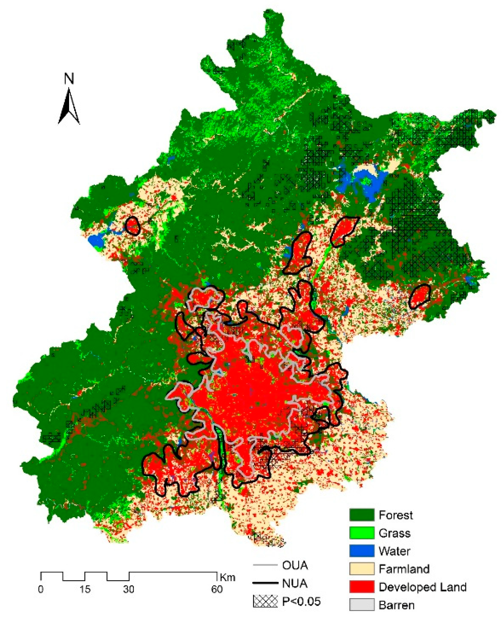
Beijing, the capital city of China, was chosen as the study area in this research (Figure 1). It is located in the northwestern part of the North China Plain (latitude: 39°28′–41°25′N, longitude: 115°25′–117°30′E) and has a monsoon-influenced humid continental climate characterized by hot and humid summers but cold and dry winters. It has an area of approximately 16,800 km2 and had a total population of more than 22 million in 2016 [61]. In recent decades, Beijing has experienced rapid urban expansion, with large areas of natural and agricultural land being converted into urban build-up areas [62], which has led to deteriorating urban heat [37,39].
2.2. Identification of Different Urban Zones
We mapped the study area into two different parts, urban areas (UA) and nonurban areas (NoUA), in 2015. Further, we subdivided UA into two different zones, namely urban areas developed before the year 2000 (hereafter referred to as old urban areas, OUA) and urban areas developed between 2000 and 2015 (hereafter referred to as new urban areas, NUA). The UA and NoUA were mapped following the methods detailed in Reference [37]. Briefly, we first created fishnets with a size of 900 m × 900 m in order to approximately match the resolution of MODerate-resolution Imaging Spectroradiometer (MODIS) products. We then calculated the percent of developed land in each fishnet in both 2000 and 2015 using a land cover dataset derived from 30-m Landsat Thematic Mapper (TM) data with an overall accuracy of over 96% [63,64]. We defined the fishnets as urbanized fishnets if the percent of developed land was greater than 50% [26,37,65]. Finally, the urbanized fishnets in 2015 were merged to generate UA, and the urbanized fishnets in 2000 were merged to generate OUA. The NUA were generated by removing OUA from UA. Relatively small land cover changes occurred in OUA from 2000 to 2015, but there were dramatic changes occurred in the NUA, where many different types of land cover (e.g., farmland, forest) were transformed into developed land.
2.3. LST, EVI, and NDBI from MODIS Products
A total of 416 images from MODIS Land Surface Temperature L3 product MOD11A2 Version 6, with a spatial resolution of 1000 m, were used in this study. The MOD11A2 product provides 8-day averaged LST based on daily LST produced by a split-window algorithm [66,67]. We calculated the mean LST for each summer (June to August) from 2000 to 2015.
We used EVI data derived from MODIS Vegetation Index L3 product MOD13A2 (224 total images, Version 6). The MOD13A2 product has a spatial resolution of 1000 m and provides a vegetation index for a 16-day time period by choosing the best available value from the 16-day period [68]. We calculated the mean EVI for each summer from 2000 to 2015. The EVI has been widely used to measure vegetation abundance [26]. It has improved sensitivity over high biomass regions and improved vegetation monitoring capability through a decoupling of the canopy background signal and a reduction in atmosphere influences [68]. NDBI data in this study were derived from MODIS Surface Reflectance L3 product MOD09A1 Version 6, with a spatial resolution of 500 m and a total of 416 images. The MOD09A1 product provides an estimate of the surface spectral reflectance of Bands 1–7, corrected for atmospheric conditions [69]. NDBI is defined as
where RSWIR and RNIR are the surface spectral reflectance of Band 6 and Band 2, respectively [70]. To match the spatial resolutions of LST and EVI data, we resampled the MOD09A1 to 1000 m and then calculated the mean NDBI for each summer from 2000 to 2015. All MODIS products used in this study from Terra were acquired at 10:30/22:30 local time [71].
NDBI = (RSWIR − RNIR)/(RSWIR + RNIR),
2.4. The Calculation of Temporal Trends for SUHII, LST, EVI, and NDBI
We first calculated SUHII at the city level for the three urban zones, namely the OUA, NUA, and UA. The SUHII for each urban zone was defined as the difference in averaged LST between the urban areas (i.e., OUA, NUA, and UA) and the nonurban areas (NoUA). We then calculated the SUHII at the pixel level for each pixel in the UA, which was the difference between the LST of each pixel in the UA and the averaged LST in the NoUA. After we obtained the data of SUHII, LST, EVI, and NDBI from 2000 to 2015, we investigated the temporal trends of such variables (e.g., SUHII) at every pixel using ordinary least squares (OLS) linear regression models [36,43,72]. Here we use TrendLST as an example to illustrate the calculation of TrendLST, TrendSUHII, TrendEVI, and TrendNDBI. We ran multiple OLS models at each pixel, with LST as the dependent variable and the year as the independent variable, to examine the regression coefficient, which was labeled as TrendLST and used to measure the trend and annual magnitude of the change in LST. We tested the significance at the 0.05 level. For example, a positive TrendLST with p < 0.05 means that LST at a specific pixel increased significantly from 2000 to 2015.
2.5. Statistics Analysis
Linear regression analysis was used to examine the temporal trends of SUHII, LST, etc., and to examine the effects of EVI and NDBI on LST across space for each year, with the NDBI and EVI as predictors and LST as the response variable. We compared the relative importance between different study zones of effects of NDBI and EVI on LST from 2000 to 2015 using standardized coefficients (i.e., beta coefficients) [49,53,73,74]. Finally, focusing only on the pixels with significant TrendEVI, TrendNDBI, and TrendLST during the daytime, we used Pearson correlation analysis and multiple linear regression to examine the effects of TrendEVI and TrendNDBI on TrendLST and the standardized coefficients to compare the relative importance of TrendEVI and TrendNDBI. Figure 2 shows a flowchart of this study.
3. Results
3.1. The Urban Heat Island Effect Was Intensified in Beijing from 2000 to 2015
There was a significant increasing trend in SUHII in urban areas (UA) from 2000 to 2015, suggesting that the UHI effect was intensified in Beijing (Figure 3). During the daytime, SUHII in UA increased from 4.35 °C in 2000 to 6.02 °C in 2015 (Figure 3), with a mean of 5.01 °C, a standard deviation of 0.70 °C (Table A1), and a rate of 0.13 °C/year (Figure 3). Compared to the daytime results, nighttime SUHII had a similar increasing trend from 2000 to 2015, but with smaller values (from 2.68 °C to 3.33 °C) (Table A1) and a rate of 0.04 °C/year (Figure 3).
Additionally, OUA and NUA had a significant increasing temporal trend of daytime SUHII from 2000 to 2015 (Figure 3 and Figure 4). Compared to OUA, the averaged daytime SUHII in NUA was smaller (5.94 °C in OUA vs. 4.27 °C in NUA) (Table A1). However, the increasing rate of daytime SUHII in NUA (0.145 °C/year) was higher than that in OUA (0.102 °C/year) (Figure 4), suggesting that NUA faced more rapid daytime warming than OUA (Figure 4). Similar patterns of nighttime SUHII were observed for OUA and NUA, but OUA had a slightly weaker trend (Figure 4).
Spatially, most of the areas in OUA had a significantly positive TrendSUHII during the daytime, except for a few locations, such as the Beijing Olympic Park, which had negative TrendSUHII (Figure 5). Compared to OUA, NUA usually had a smaller mean but a larger standard deviation of SUHII from 2000 to 2015 (Table A1). Additionally, NUA had large proportional areas with a higher increasing rate of TrendSUHII, especially in the southeast UA (Figure 5). Similarly, most of the areas in UA had a positive TrendSUHII during the nighttime (Figure 6), and NUA usually had large proportional areas with a higher increasing rate of TrendSUHII (Figure 6) compared to OUA and UA. Obviously, SUHII was usually lower at nighttime than daytime both in NUA and OUA (Figure 5 and Figure 6).
3.2. The Rate of Cooling in Nonurban Areas Was Larger than the Rate of Warming in Urban Areas
This significant increasing trend of averaged SUHII in UA, however, was largely caused by the cooling trend in NoUA because of their relatively larger magnitudes of the cooling rate, although it was also strengthened by the relatively weak warming trend in UA (Figure 3). The daytime LST in UA had a very weak increasing trend, with a rate of 0.04 °C from 2000 to 2015 (Figure 3c). In contrast, there was a stronger trend in the decrease of LST in NoUA, with an annual cooling rate of 0.08 °C (Figure 3c). Consequently, there was a significant increasing trend in SUHII in UA (Figure 3a). Similarly, a warming trend (i.e., positive TrendLST) was observed in UA, but a cooling trend (i.e., negative TrendLST) with a greater rate occurred in NoUA, which led to an increase of SUHII in UA during nighttime (Figure 3b,d).
Both OUA and NUA had significant increasing trends of daytime SUHII from 2000 to 2015 (Figure 4c). Compared to OUA, the averaged SUHII in NUA was smaller (Table A1). However, the increasing rate of SUHII in NUA (0.15 °C/year) was higher than that in OUA (0.10 °C/year) (Figure 4a), suggesting that NUA faced more rapid warming than OUA did (Figure 4a). The OUA had a very weak trend in LST increase (0.02 °C/year), whereas NUA had a stronger warming trend (0.06 °C/year) during the daytime (Figure 4c). Such warming rates, however, were both smaller than the cooling rate in NoUA (0.08 °C/year) (Figure 4c). Therefore, the intensified SUHII was largely due to the cooling in NoUA and also due to the relatively weak warming in both OUA and NUA. Ultimately, the cooling rate in NoUA outweighed the warming rate in the NUA and OUA and resulted in an increasing trend of SUHII in the two suburban areas (Figure 4a,c). During nighttime, similar patterns were observed for OUA and NUA, but NUA had a slightly weaker increasing trend of LST during nighttime (Figure 4).
Spatially, there were large variations in significant warming and cooling spots for the entire study area, as well for different zones (Figure 7 and Figure 8). During the daytime, most UA had positive TrendLST (Figure 7a,c,d), while only a few spots, such as the Beijing Olympic Park, had a negative TrendLST in OUA (Figure 7a,b). The area percentage of significant warming in UA (15.28%) and OUA (5.81%) was smaller than that of significant cooling in NoUA (15.96%), except for NUA with a large proportion of the zone (22.80%) having a significant increase in TrendLST (Figure 7a,d). Additionally, the averaged significant cooling rate in NoUA was 0.17 °C/year, similar to the warming rate in OUA, although smaller than that in NUA (0.21 °C/year) and UA (0.20 °C/year) (Figure 7e).
The spatial pattern of TrendLST from 2000 to 2015 during the nighttime, however, was largely different from that during the daytime (Figure 8). One of the most noticeable difference was that a much larger proportion of the entire study area had a positive TrendLST during the nighttime compared to during the daytime (Figure 7a, Figure 8a). The area percent of urban warming in UA (OUA and NUA included) was similar to that of cooling in NoUA (Figure 8b) and similar to the comparison of averaged magnitudes (Figure 8c).
3.3. The Trends of EVI and NDBI Significantly Affected LST Trends
Most of the NoUA had a positive TrendEVI from 2000 to 2015, with 46.11% of the areas having a significant trend, with EVI increasing (Figure 9). Both the OUA and NUA had large area percentages with positive TrendNDBI during this period (Figure 9). The percentage of areas in NUA experienced a significant increasing trend in NDBI was 45.12%, which was larger than that in OUA (22.14%) (Figure 9), suggesting that more areas in NUA faced with quick urbanization that natural land was transformed to impervious area. In contrast, the percentage of areas in OUA had a significant increasing trend (i.e., significantly positive TrendEVI) was 54.74%, which was larger than that in NUA (18.84%), and even NoUA (Figure 9). Spatially, EVI increased where NDBI decreased, especially in urban areas (i.e., NUA).
The results from OLS multiple linear regressions, with NDBI and EVI as the predictors and LST as the response variable, showed that in all analytical areas, EVI had significantly negative effects on LST, while NDBI had positive effects every year from 2000 to 2015. However, their relative importance on affecting LST varied by zones and changed over time (Table 1). In UA, EVI and NDBI played a nearly equally important role in predicting LST, and their relative importance remained largely unchanged over time, as indicated by the standardized coefficients (Table 1). In contrast, in surrounding NoUA, NDBI played a much more important role in predicting LST than EVI did, similarly to NUA (Table 1). On the contrary, in OUA, EVI played a more important role than NDBI did from 2000 to 2004, and then the two factors played a similar role in predicting LST (Table 1) Larger variations in LST were explained jointly by EVI and NDBI in OUA than NUA (Table 1). As for R2 in UA and NoUA, in the first few years, R2 values were larger in UA, but after 2009, the opposite was found.
We further explored how the changes in EVI and NDBI influenced LST, considering the pixels with significant TrendEVI, TrendNDBI, and TrendLST (Figure 10). For pixels with significantly positive TrendLST, TrendEVI had a significantly negative relationship with TrendLST, while TrendNDBI had a significantly positive one (Figure 11). This result suggested that the magnitudes of temporal trends of EVI and NDBI would significantly affect the magnitude of the temporal trend of LST in long-term time series. Decreased LST (TrendLST < 0) was related to increased EVI (TrendEVI > 0) and decreased NDBI (TrendNDBI < 0) significantly, meaning that LST would decrease when EVI increased and NDBI decreased significantly (Figure 11). A positive relationship between TrendNDBI and TrendLST was found, indicating that a higher TrendNDBI was related to a higher TrendLST (Figure 10). Interestingly, TrendEVI had a weak but significantly positive relationship with TrendLST (p = 0.023), which was different from the negative relationship between those two when TrendEVI was negative. This result indicated that an increase in EVI would lead to a decrease in LST. However, a more rapid increase of EVI did not lead to a more rapid decrease of LST. In fact, the larger increasing rate of EVI was associated with a slower decreasing rate of LST. In addition, TrendNDBI was a more important predictor of TrendLST, playing a much more important role in predicting TrendLST than TrendEVI, as suggested by the standard coefficients (Table 2).
4. Discussion
4.1. Understanding the Process of Intensified SUHII by Comparing the Differences in LST Trends in Urban and Nonurban Areas
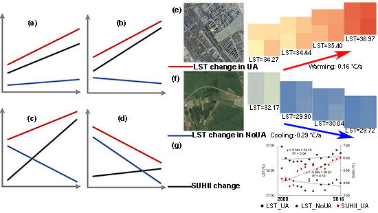
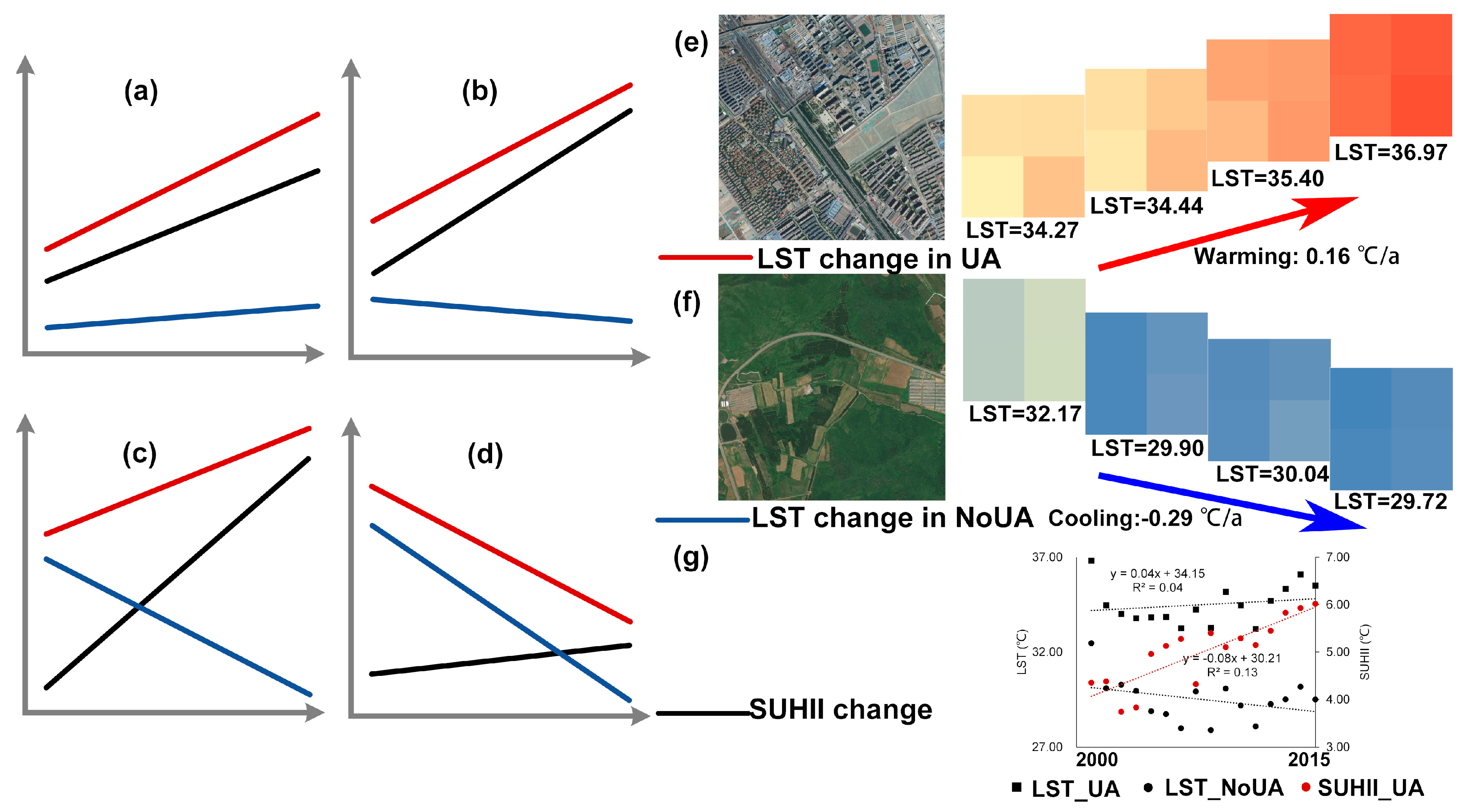
The Beijing metropolitan area had intensified SUHI, as suggested by the increasing trend of SUHII from 2000–2015. This result is consistent with that from a large amount of studies, which found that with urban expansion, the UHII (both SUHII and UHII in terms of air temperature) tends to increase [33,37,39,41,43,60,72,76,77,78]. Compared to old urban areas (OUA in this study), the new urbanized and urbanizing areas (NUA in this study) had a more rapid intensification of UHI, which was indicated by both the SUHII and LST values, similarly to findings from previous results [34,42,60,79]. What is new in this study is that we further revealed that such intensification in Beijing was largely due to the cooling trend in surrounding nonurban areas but not due to significant warming in urban areas. While both the cooling trend in nonurban areas and the warming trend in urban areas contributed to such intensification, the magnitude of the cooling rate in nonurban areas was much larger than that of the warming rate in urban areas. This result has significant implications for urban heat mitigation and adaptation. The cooling trend in the surrounding nonurban areas was likely due to the ecological restoration projects conducted in Beijing, especially the Million Mu Trees Campaign, which greatly increased the coverage of forests [80]. While the urban areas from 2000–2015 overall had an increasing LST trend, a relatively large proportion (38.50%) of OUA had a trend of cooling. This was likely due to increased efforts dedicated to urban greening in Beijing, such as the “Plant Where Possible” policy in the urban core areas [81,82], which have led to the establishment of lots of new urban vegetation and parks in old urban areas [81,83]. Such greening efforts can help reduce LST in urban areas [53,54,59,84]. However, LST in the new urban areas generally had a trend of increase, and at a higher rate compared to old urban areas. Urban expansion, especially edge expansion and leapfrogging in NUA [75,85,86], typically includes replacing vegetation and natural land with impervious surfaces, which changes characteristics toward lower albedo, more anthropogenic heat (e.g., more cars, more air conditioning), higher heat storage (e.g., more tall buildings), and lower evapotranspiration in urban areas [87,88,89,90]. These changes thereby lead to the increase of LST. However, it is worth noting that even though LST had an increasing trend in the new urban areas, the annual warming rate was small (Figure 4). This was also a result of the great efforts that Beijing has devoted to urban greening. For example, a regulation was enforced in 2010 that requires that the percentage cover of vegetation be greater than 30% in all newly built residential areas.
Our study underscores the importance for urban heat mitigation strategies of quantifying and reporting the temporal trends of LST in both urban and surrounding nonurban areas when investigating SUHI and its changes. Such points have been conducted in previous studies [33,36], which found significantly intensified SUHII but with different LST changes between urban and nonurban areas [33,36], and also revealed that the cooling in rural areas (e.g., because of EVI enhancement) could explain such intensified SUHII (e.g., around 22.5%) [35]. What’s new in this study is that we further gave four potential scenarios that have intensified SUHII based on a comparison between LST change in urban and nonurban areas: (a) LST increased in both urban and nonurban areas, but at a greater magnitude of warming rate in urban areas (Figure 12a); (b) the LST in urban areas increased, while it decreased in nonurban areas. The warming rate in urban areas outweighed the cooling rate in surrounding nonurban areas (Figure 12b). (c) The LST in urban areas increased, while it decreased in nonurban areas. The cooling rate in surrounding nonurban areas outweighed the warming rate in urban areas (Figure 12c). (d) The LST decreased in both urban and nonurban areas, but at a greater magnitude of cooling in nonurban areas (Figure 12d). While SUHII may increase along with urbanization, as has been shown in many previous studies, intensified SUHI as a result of scenario d would be the best (and scenario a would be the worst) from the perspective of urban sustainable development. Our classification differed from the classification which was based on seasonal and diurnal variations of LST changes in Reference [36]. Our classification, which focused on the LST changes in both urban and nonurban areas, could be more important for specific cities in city-based urban heat mitigation strategies designing.
The changes in urban temperature were the results of warming (e.g., urban heat island) and cooling effects (e.g., urban cool island) in urban areas [28,37]. A warming effect due to urban expansion (both in the horizontal and vertical dimensions, and both in urban land intensification and urban population concentration) may lead to an increase in temperature in urban areas. Meanwhile, increased vegetation cover due to the great efforts of urban greening policies [81], plus vegetation management such as irrigation [28], can result in a decrease in temperature. Changes in temperature depend on the net effects of warming and cooling [28]. Similarly, rapid urbanization could increase temperature in nonurban areas because of the strong effect of urban areas on surrounding nonurban areas, such as great changes in rural landscapes [41]. Meanwhile, along with urbanization, the migration of rural populations to urban areas and great greening polices lead to the restoration of ecosystems in nonurban areas, which can make the nonurban area temperatures lower [91]. Changes in temperature in rural areas depend on the net effects of these two opposite processes as well.
In scenario d (as an example), an increase in SUHII is the result of a decrease in temperature in both urban and rural areas. In contrast, in scenario a, an increase in SUHII is the result of an increase in temperature in both urban and rural areas. While the trends in SUHII are similar, that is, increases in both scenarios, a and d, their implications for human health and urban and regional sustainability are totally different. Beijing generally fits in scenario c, with a smaller magnitude of warming rate in urban areas than in the cooling rate in nonurban areas. This is likely due to greening efforts dedicated to urban areas [81], which can effectively alleviate the continuous increase of urban temperatures. These great greening polices, which lead to the restoration of ecosystems in rural areas, can make the temperature lower in nonurban areas as well [91].
The classification of cities into one of the four types with increasing SUHIIs could provide more information on urban heat and help promulgate greening regulations according to the specific conditions of urban and rural areas. It should be noted that the classification of a city into one of the types may vary by the environmental context of a specific city and may change with time (daytime or nighttime or in different seasons). Therefore, cross-city comparison research would be desirable in future studies to design city-based heat mitigation strategies.
4.2. Understanding the Effect of Land Cover Changes on LST Change by Using Long-Term Time Series Data
EVI and NDBI both significantly affected LST. However, their relative importance in predicting LST varied by zone and year. Our results show that NDBI played a more important role in predicting LST in new urban areas and surrounding nonurban regions, which is similar to findings from previous studies [57,92]. Many previous studies found that impervious abundance index, such as NDBI or percent cover of impervious surface area (ISA), was more important than vegetation abundance index, such as EVI, the normalized vegetation index (NDVI), or percent cover of vegetation [57,92,93,94,95]. The relative importance of the two variables, however, was different in old urban areas. EVI generally played a slightly more important role in predicting LST than NDBI did in old urban areas (Table 1). Old urban areas in Beijing typically have less vegetation coverage than new urban areas and surrounding nonurban regions [63,81]. This result may suggest that increasing vegetation coverage in old urban areas could lead to better cooling effects [53]. Additionally, although increasing vegetation generally could lower LST, the relationship between vegetation and LST varied spatially across the city. Such variation may be related to other characteristics of vegetation (e.g., quality) in addition to the amount of vegetation [96]. For example, previous studies have shown that local climate zones can be a useful tool in exploring the relationship between vegetation and LST by considering the different vegetation classes in terms of height and density of vegetation [97]. Future research that uses local climate zones to better understand the relationship between EVI and LST is highly desirable.
Additionally, the temporal trend of EVI and NDBI could also lead to LST variability (significantly). Our results showed that TrendEVI was negatively related to TrendLST only when EVI decreased, which was consistent with results from previous studies [44,60], indicating that the higher the rate of the loss of existing urban vegetation was, the more rapid the LST increase was [60]. However, our results also showed that TrendEVI positively affected TrendLST significantly when EVI increased (i.e., TrendEVI was positive), which was slightly different from the results found in Wang et al., 2016 [60], suggesting that the magnitude of increase of new urban vegetation might not result in the same amount of magnitude decrease in LST. In other words, with an increase in new urban vegetation, its effects on or capacity to lower LST declined. This was likely due to the fact that newly generated urban vegetation did not have the same cooling capacity as the the existing vegetation did [59]. For example, compared to mature trees, newly planted trees generally are shorter and have less tree canopy coverage, and therefore the same amount of vegetation may provide less shading and evapotranspiration but may lead to a decrease in albedo because of more underlying bared soil. Consequently, although a gain in trees could ameliorate urban heat, if we just focus on an increase in the amount of urban vegetation, such as creating new urban vegetation rapidly, the cooling effect will not be high as we expect [59]. These results highlight the importance of not only considering increases in the amount of vegetation, but also improving its quality [54,98].
We also found that the change in NDBI played a much more important role in predicting LST change than did the change in EVI. These results were different from previous work that showed that a cooling effect of increased vegetation cover was actually stronger than the heating effect due to urban development and expansion [60]. However, it should be noted that Wang et al. (2016) focused on two time slices (i.e., 2000 and 2014), but we used the temporal trends of EVI and NDBI from a time series of remote sensing data, which could potentially reduce the effects just from one or two years. It should be noted that although aggregating LST to a summer mean level greatly increased the spatial coverage of LST pixels, it reduced the temporal resolution of the LST data, and thus could have potentially resulted in information loss compared to the use of entire LST scenes individually.
5. Conclusions
This study aimed to reveal whether the intensification of SUHI is mainly caused by urban warming or the cooling of surrounding nonurban regions and to investigate the potential drivers of LST change. Using time-series analysis, we found that (1) there was a significant increasing trend in SUHII from 2000 to 2015, suggesting intensified SUHI effects in Beijing, especially in OUA. (2) This significant intensified SUHII, however, was largely due to a cooling trend in the NoUA, not to significant warming in UA. While both the cooling trend in NoUA and the warming trend in UA contributed to such intensification, the magnitude of cooling in NoUA contributed much more to the intensification than did warming in the UA. Spatially, there was a smaller percentage of areas with significant urban warming in OUA than the percentage of areas with significant cooling in NoUA. Locations with cooling trends also occurred in UA, particularly in OUA. (3) The EVI and NDBI could affect LST significantly (negatively and positively, respectively), but with varied importance in different study zones and time. (4) TrendEVI significantly affected TrendLST positively when EVI increased, suggesting that a more rapid increase in new urban vegetation (EVI increase) could lead to a slower decrease in LST but not to a quicker decrease in LST, as we expected.
This study also presents a research framework that underscored the importance for urban heat mitigation strategies of comparing and reporting the temporal trends of LST in both urban and surrounding nonurban areas when investigating SUHII and its changes. The framework highlighted that it is not enough to focus on SUHII and its changes alone, which might even be misleading. It also suggests that this is necessary for city-based urban heat mitigation strategies. This is because an intensified SUHI may be caused by totally different warming/cooling processes in urban and nonurban areas. Therefore, more city-based research and cross-city comparisons are highly desirable. Additionally, this study also enhances our understanding of evidence and the drivers of intensified urban heat island effects.
Author Contributions
Conceptualization, W.Z. and J.W. (Jia Wang); formal analysis, J.W. (Jia Wang) and J.W. (Jing Wang); writing—original draft preparation, J.W. (Jia Wang) and W.Z.; writing—review and editing, W.Z.
Funding
This research was funded by the National Natural Science Foundation of China (Grant No. 41771203, 41422104, 41601180), and the Key Research Program of Frontier Sciences, Chinese Academy of Sciences (CAS) (Grant No. QYZDB-SSW-DQC034).
Acknowledgments
The authors thank the anonymous reviewers for their constructive comments and suggestions.
Conflicts of Interest
The authors declare no conflict of interest.
Variables and Acronyms
| SUHII | Surface urban heat island intensity |
| UA | Urban areas, urban areas developed before 2015 |
| OUA | Old urban areas, urban areas developed before the year 2000 |
| NUA | Nonurban areas, rural areas that were not urbanized before the year 2015 |
| NoUA | Nonurban areas, rural areas that were not urbanized before the year 2015 |
| TrendSUHII | Temporal trend (i.e., the coefficient) of SUHII from 2000 to 2015, both at a city and pixel level |
| TrendLST | Temporal trend (i.e., the coefficient) of LST from 2000 to 2015, both at a city and pixel level |
| TrendNDBI | Temporal trend (i.e., the coefficient) of NDBI from 2000 to 2015 at a pixel level |
| TrendEVI | Temporal trend (i.e., the coefficient) of EVI from 2000 to 2015 at a pixel level |
Appendix A

Table A1.
The statistics, including mean and standard errors, for SUHII from 2000 to 2015 in UA, OUA, and NUA. For example, Mean_UA and std_UA mean the mean value and standard errors of SUHII in UA in different years during the day and at night.
Table A1.
The statistics, including mean and standard errors, for SUHII from 2000 to 2015 in UA, OUA, and NUA. For example, Mean_UA and std_UA mean the mean value and standard errors of SUHII in UA in different years during the day and at night.
| Year | Day | Night | ||||||||||
|---|---|---|---|---|---|---|---|---|---|---|---|---|
| Mean_UA | std_UA | Mean_OUA | std_OUA | Mean_NUA | std_NUA | Mean_UA | std_UA | Mean_OUA | std_OUA | Mean_NUA | std_NUA | |
| 2000 | 4.38 | 1.74 | 5.42 | 1.24 | 3.52 | 1.62 | 2.72 | 1.32 | 3.75 | 1.08 | 1.86 | 0.79 |
| 2001 | 4.42 | 1.65 | 5.59 | 1.19 | 3.45 | 1.31 | 2.94 | 1.27 | 3.96 | 1.02 | 2.10 | 0.72 |
| 2002 | 3.77 | 1.42 | 4.81 | 1.07 | 2.92 | 1.04 | 2.64 | 1.27 | 3.60 | 1.03 | 1.82 | 0.80 |
| 2003 | 3.86 | 1.39 | 4.70 | 1.14 | 3.18 | 1.17 | 2.91 | 1.27 | 3.94 | 0.95 | 2.05 | 0.78 |
| 2004 | 5.01 | 1.60 | 6.24 | 1.23 | 4.00 | 1.04 | 3.14 | 1.26 | 4.10 | 1.04 | 2.35 | 0.77 |
| 2005 | 5.18 | 1.48 | 6.24 | 1.12 | 4.30 | 1.10 | 3.22 | 1.23 | 4.20 | 0.97 | 2.40 | 0.74 |
| 2006 | 5.32 | 1.40 | 6.20 | 1.19 | 4.60 | 1.09 | 3.13 | 1.15 | 3.97 | 0.98 | 2.43 | 0.72 |
| 2007 | 4.36 | 1.35 | 5.24 | 1.10 | 3.64 | 1.05 | 3.18 | 1.18 | 4.08 | 0.94 | 2.43 | 0.76 |
| 2008 | 5.46 | 1.51 | 6.39 | 1.32 | 4.70 | 1.16 | 3.17 | 1.20 | 3.97 | 1.06 | 2.51 | 0.84 |
| 2009 | 5.15 | 1.35 | 5.98 | 1.09 | 4.47 | 1.11 | 3.20 | 1.35 | 4.25 | 1.08 | 2.32 | 0.82 |
| 2010 | 5.34 | 1.24 | 5.99 | 1.05 | 4.81 | 1.10 | 3.50 | 1.39 | 4.51 | 1.18 | 2.66 | 0.91 |
| 2011 | 5.20 | 1.30 | 5.92 | 1.16 | 4.61 | 1.05 | 3.59 | 1.19 | 4.47 | 0.98 | 2.86 | 0.77 |
| 2012 | 5.51 | 1.41 | 6.31 | 1.20 | 4.85 | 1.19 | 3.33 | 1.37 | 4.36 | 1.18 | 2.47 | 0.80 |
| 2013 | 5.88 | 1.33 | 6.62 | 1.10 | 5.28 | 1.16 | 3.25 | 1.37 | 4.27 | 1.17 | 2.40 | 0.86 |
| 2014 | 5.99 | 1.49 | 6.90 | 1.12 | 5.23 | 1.30 | 3.28 | 1.20 | 4.18 | 0.87 | 2.53 | 0.89 |
| 2015 | 6.08 | 1.53 | 6.82 | 1.24 | 5.49 | 1.46 | 3.37 | 1.20 | 4.27 | 0.90 | 2.62 | 0.85 |
| Averaged | 5.01 | 0.70 | 5.94 | 0.65 | 4.27 | 0.77 | 3.12 | 0.26 | 4.11 | 0.25 | 2.34 | 2.34 |
References
- United Nations. World Urbanization Prospects, the 2014 Revision; United Nations: New York, NY, USA, 2014. [Google Scholar]
- Anna, A.S.; Darryn, W.W.; Ben, F.Z. Reduced urban heat island intensity under warmer conditions. Environ. Res. Lett. 2018, 13, 064003. [Google Scholar]
- Grimm, N.B.; Faeth, S.H.; Golubiewski, N.E.; Redman, C.L.; Wu, J.; Bai, X.; Briggs, J.M. Global change and the ecology of cities. Science 2008, 319, 756. [Google Scholar] [CrossRef] [PubMed]
- Seto, K.C.; Güneralp, B.; Hutyra, L.R. Global forecasts of urban expansion to 2030 and direct impacts on biodiversity and carbon pools. Proc. Natl. Acad. Sci. USA 2012, 109, 16083–16088. [Google Scholar] [CrossRef] [PubMed] [Green Version]
- Findell, K.L.; Berg, A.; Gentine, P.; Krasting, J.P.; Lintner, B.R.; Malyshev, S.; Santanello, J.A.; Shevliakova, E. The impact of anthropogenic land use and land cover change on regional climate extremes. Nat. Commun. 2017, 8, 989. [Google Scholar] [CrossRef] [PubMed]
- Foley, J.A.; Defries, R.; Asner, G.P.; Barford, C.; Bonan, G.; Carpenter, S.R.; Chapin, F.S.; Coe, M.T.; Daily, G.C.; Gibbs, H.K. Global consequences of land use. Science 2005, 309, 570–574. [Google Scholar] [CrossRef] [PubMed]
- Kalnay, E.; Cai, M. Impact of urbanization and land-use change on climate. Nature 2003, 423, 528–531. [Google Scholar] [CrossRef]
- Han, L.; Zhou, W.; Li, W. City as a major source area of fine particulate (pm2.5) in china. Environ. Pollut. 2015, 206, 183–187. [Google Scholar] [CrossRef] [PubMed]
- Howard, L. Climate of London Deduced from Metrological Observations; Harvey and Dorton Press: London, UK, 1833; Volume 1. [Google Scholar]
- Peng, S.; Piao, S.; Ciais, P.; Friedlingstein, P.; Ottle, C.; Bréon, F.-M.; Nan, H.; Zhou, L.; Myneni, R.B. Surface urban heat island across 419 global big cities. Environ. Sci. Technol. 2012, 46, 696–703. [Google Scholar] [CrossRef]
- Voogt, J.A.; Oke, T.R. Thermal remote sensing of urban climates. Remote Sens. Environ. 2003, 86, 370–384. [Google Scholar] [CrossRef]
- Zhao, L.; Lee, X.; Smith, R.B.; Oleson, K. Strong contributions of local background climate to urban heat islands. Nature 2014, 511, 216. [Google Scholar] [CrossRef]
- Santamouris, M.; Cartalis, C.; Synnefa, A.; Kolokotsa, D. On the impact of urban heat island and global warming on the power demand and electricity consumption of buildings—A review. Energy Build. 2015, 98, 119–124. [Google Scholar] [CrossRef]
- Santamouris, M.; Papanikolaou, N.; Livada, I.; Koronakis, I.; Georgakis, C.; Argiriou, A.; Assimakopoulos, D.N. On the impact of urban climate on the energy consumption of buildings. Solar Energy 2001, 70, 201–216. [Google Scholar] [CrossRef]
- Zhou, D.; Xiao, J.; Bonafoni, S.; Berger, C.; Deilami, K.; Zhou, Y.; Frolking, S.; Yao, R.; Qiao, Z.; Sobrino, J.A. Satellite remote sensing of surface urban heat islands: Progress, challenges, and perspectives. Remote Sens. 2019, 11, 48. [Google Scholar] [CrossRef]
- White, M.A.; Nemani, R.R.; Thornton, P.E.; Running, S.W. Satellite evidence of phenological differences between urbanized and rural areas of the eastern united states deciduous broadleaf forest. Ecosystems 2002, 5, 260–273. [Google Scholar] [CrossRef]
- Niemelä, J. Ecology and urban planning. Biodivers. Conserv. 1999, 8, 119–131. [Google Scholar] [CrossRef]
- Akbari, H.; Pomerantz, M.; Taha, H. Cool surfaces and shade trees to reduce energy use and improve air quality in urban areas. Solar Energy 2001, 70, 295–310. [Google Scholar] [CrossRef]
- Akbari, H.; Rosenfeld, A.; Taha, H.; Gartland, L. Mitigation of summer urban heat islands to save electricity and smog. In Proceedings of the 76th Annual Meteorological Society Meeting, Atlanta, GA, USA, 28 January–2 February 1996. [Google Scholar]
- Patz, J.A.; Campbell-Lendrum, D.; Holloway, T.; Foley, J.A. Impact of regional climate change on human health. Nature 2005, 438, 310. [Google Scholar] [CrossRef] [PubMed]
- Poumadere, M.; Mays, C.; Le Mer, S.; Blong, R. The 2003 heat wave in France: Dangerous climate change here and now. Risk Anal. 2005, 25, 1483–1494. [Google Scholar] [CrossRef]
- Li, G.; Zhang, X.; Mirzaei, P.A.; Zhang, J.; Zhao, Z. Urban heat island effect of a typical valley city in china: Responds to the global warming and rapid urbanization. Sustain. Cities Soc. 2018, 38, 736–745. [Google Scholar] [CrossRef]
- Ramamurthy, P.; Sangobanwo, M. Inter-annual variability in urban heat island intensity over 10 major cities in the United States. Sustain. Cities Soc. 2016, 26, 65–75. [Google Scholar] [CrossRef]
- Tran, H.; Uchihama, D.; Ochi, S.; Yasuoka, Y. Assessment with satellite data of the urban heat island effects in asian mega cities. Int. J. Appl. Earth Observ. Geoinf. 2006, 8, 34–48. [Google Scholar] [CrossRef]
- Zhou, D.; Bonafoni, S.; Zhang, L.; Wang, R. Remote sensing of the urban heat island effect in a highly populated urban agglomeration area in east china. Sci. Total Environ. 2018, 628, 415–429. [Google Scholar] [CrossRef] [PubMed]
- Zhou, D.; Zhao, S.; Liu, S.; Zhang, L.; Zhu, C. Surface urban heat island in china’s 32 major cities: Spatial patterns and drivers. Remote Sens. Environ. 2014, 152, 51–61. [Google Scholar] [CrossRef]
- Wang, J.; Huang, B.; Fu, D.; Atkinson, P.M. Spatiotemporal variation in surface urban heat island intensity and associated determinants across major Chinese cities. Remote Sens. 2015, 7, 3670. [Google Scholar] [CrossRef]
- Cui, Y.; Xiao, X.; Doughty, R.B.; Qin, Y.; Liu, S.; Li, N.; Zhao, G.; Dong, J. The relationships between urban-rural temperature difference and vegetation in eight cities of the Great Plains. Front. Earth Sci. 2018, 13, 290–302. [Google Scholar] [CrossRef]
- Gallo, K.P.; McNab, A.L.; Karl, T.R.; Brown, J.F.; Hood, J.J.; Tarpley, J.D. The use of NOAA AVHRR data for assessment of the urban heat island effect. J. Appl. Meteorol. 1993, 32, 899–908. [Google Scholar] [CrossRef]
- Cai, G.; Du, M.; Xue, Y. Monitoring of urban heat island effect in Beijing combining aster and tm data. Int. J. Remote Sens. 2011, 32, 1213–1232. [Google Scholar] [CrossRef]
- Li, H.; Zhou, Y.; Li, X.; Meng, L.; Wang, X.; Wu, S.; Sodoudi, S. A new method to quantify surface urban heat island intensity. Sci. Total Environ. 2018, 624, 262–272. [Google Scholar] [CrossRef] [PubMed]
- Chen, X.-L.; Zhao, H.-M.; Li, P.-X.; Yin, Z.-Y. Remote sensing image-based analysis of the relationship between urban heat island and land use/cover changes. Remote Sens. Environ. 2006, 104, 133–146. [Google Scholar] [CrossRef]
- Zhou, D.; Zhang, L.; Hao, L.; Sun, G.; Liu, Y.; Zhu, C. Spatiotemporal trends of urban heat island effect along the urban development intensity gradient in china. Sci. Total Environ. 2016, 544, 617–626. [Google Scholar] [CrossRef]
- Yao, R.; Wang, L.; Huang, X.; Niu, Z.; Liu, F.; Wang, Q. Temporal trends of surface urban heat islands and associated determinants in major Chinese cities. Sci. Total Environ. 2017, 609, 742–754. [Google Scholar] [CrossRef] [PubMed]
- Yao, R.; Wang, L.; Huang, X.; Gong, W.; Xia, X. Greening in rural areas increases the surface urban heat island intensity. Geophys. Res. Lett. 2019, 46, 2204–2212. [Google Scholar] [CrossRef]
- Peng, J.; Ma, J.; Liu, Q.; Liu, Y.; Hu, Y.N.; Li, Y.; Yue, Y. Spatial-temporal change of land surface temperature across 285 cities in china: An urban-rural contrast perspective. Sci. Total Environ. 2018, 635, 487–497. [Google Scholar] [CrossRef] [PubMed]
- Hu, X.; Zhou, W.; Qian, Y.; Yu, W. Urban expansion and local land-cover change both significantly contribute to urban warming, but their relative importance changes over time. Landsc. Ecol. 2017, 32, 763–780. [Google Scholar] [CrossRef]
- Liu, W.; Ji, C.; Zhong, J.; Jiang, X.; Zheng, Z. Temporal characteristics of the Beijing urban heat island. Theor. Appl. Climatol. 2007, 87, 213–221. [Google Scholar] [CrossRef]
- Meng, Q.; Zhang, L.; Sun, Z.; Meng, F.; Wang, L.; Sun, Y. Characterizing spatial and temporal trends of surface urban heat island effect in an urban main built-up area: A 12-year case study in Beijing, China. Remote Sens. Environ. 2017, 204, 826–837. [Google Scholar] [CrossRef]
- Quan, J.; Chen, Y.; Zhan, W.; Wang, J.; Voogt, J.; Wang, M. Multi-temporal trajectory of the urban heat island centroid in Beijing, china based on a Gaussian volume model. Remote Sens. Environ. 2014, 149, 33–46. [Google Scholar] [CrossRef]
- Wang, H.; Zhang, Y.; Tsou, J.; Li, Y. Surface urban heat island analysis of shanghai (china) based on the change of land use and land cover. Sustainability 2017, 9, 1538. [Google Scholar] [CrossRef]
- Shen, H.; Huang, L.; Zhang, L.; Wu, P.; Zeng, C. Long-term and fine-scale satellite monitoring of the urban heat island effect by the fusion of multi-temporal and multi-sensor remote sensed data: A 26-year case study of the city of Wuhan in china. Remote Sens. Environ. 2016, 172, 109–125. [Google Scholar] [CrossRef]
- Polydoros, A.; Mavrakou, T.; Cartalis, C. Quantifying the trends in land surface temperature and surface urban heat island intensity in Mediterranean cities in view of smart urbanization. Urban Sci. 2018, 2, 16. [Google Scholar] [CrossRef]
- Yao, R.; Wang, L.; Huang, X.; Zhang, W.; Li, J.; Niu, Z. Interannual variations in surface urban heat island intensity and associated drivers in china. J. Environ. Manag. 2018, 222, 86–94. [Google Scholar] [CrossRef] [PubMed]
- Wang, W.; Zhou, W.; Ng, E.Y.Y.; Xu, Y. Urban heat islands in Hong Kong: Statistical modeling and trend detection. Nat. Hazards 2016, 83, 885–907. [Google Scholar] [CrossRef]
- Ren, G.Y.; Chu, Z.Y.; Chen, Z.H.; Ren, Y.Y. Implications of temporal change in urban heat island intensity observed at Beijing and Wuhan stations. Geophys. Res. Lett. 2007, 34. [Google Scholar] [CrossRef]
- Fu, P.; Weng, Q. A time series analysis of urbanization induced land use and land cover change and its impact on land surface temperature with Landsat imagery. Remote Sens. Environ. 2016, 175, 205–214. [Google Scholar] [CrossRef]
- Huang, G.; Cadenasso, M.L. People, landscape, and urban heat island: Dynamics among neighborhood social conditions, land cover and surface temperatures. Landsc. Ecol. 2016, 31, 2507–2515. [Google Scholar] [CrossRef]
- Zhou, W.Q.; Huang, G.L.; Cadenasso, M.L. Does spatial configuration matter? Understanding the effects of land cover pattern on land surface temperature in urban landscapes. Landsc. Urban Plan. 2011, 102, 54–63. [Google Scholar] [CrossRef]
- Imhoff, M.L.; Zhang, P.; Wolfe, R.E.; Bounoua, L. Remote sensing of the urban heat island effect across biomes in the continental USA. Remote Sens. Environ. 2010, 114, 504–513. [Google Scholar] [CrossRef] [Green Version]
- Jenerette, G.D.; Harlan, S.L.; Brazel, A.; Jones, N.; Larsen, L.; Stefanov, W.L. Regional relationships between surface temperature, vegetation, and human settlement in a rapidly urbanizing ecosystem. Landsc. Ecol. 2007, 22, 353–365. [Google Scholar] [CrossRef]
- Li, X.X.; Li, W.W.; Middel, A.; Harlan, S.; Brazel, A.; Turner, B. Remote sensing of the surface urban heat island and land architecture in Phoenix, Arizona: Combined effects of land composition and configuration and cadastral–demographic–economic factors. Remote Sens. Environ. 2016, 174, 233–243. [Google Scholar] [CrossRef]
- Zhou, W.; Wang, J.; Cadenasso, M.L. Effects of the spatial configuration of trees on urban heat mitigation: A comparative study. Remote Sens. Environ. 2017, 195, 1–12. [Google Scholar] [CrossRef]
- Bowler, D.E.; Buyung-Ali, L.; Knight, T.M.; Pullin, A.S. Urban greening to cool towns and cities: A systematic review of the empirical evidence. Landsc. Urban Plan. 2010, 97, 147–155. [Google Scholar] [CrossRef]
- Connors, J.P.; Galletti, C.S.; Chow, W.T.L. Landscape configuration and urban heat island effects: Assessing the relationship between landscape characteristics and land surface temperature in Phoenix, Arizona. Landsc. Ecol. 2013, 28, 271–283. [Google Scholar] [CrossRef]
- Li, X.M.; Zhou, W.Q.; Ouyang, Z.Y.; Xu, W.H.; Zheng, H. Spatial pattern of greenspace affects land surface temperature: Evidence from the heavily urbanized Beijing metropolitan area, china. Landsc. Ecol. 2012, 27, 887–898. [Google Scholar] [CrossRef]
- Zhou, W.Q.; Qian, Y.G.; Li, X.M.; Li, W.F.; Han, L.J. Relationships between land cover and the surface urban heat island: Seasonal variability and effects of spatial and thematic resolution of land cover data on predicting land surface temperatures. Landsc. Ecol. 2014, 29, 153–167. [Google Scholar] [CrossRef]
- Li, J.X.; Song, C.H.; Cao, L.; Zhu, F.G.; Meng, X.L.; Wu, J.G. Impacts of landscape structure on surface urban heat islands: A case study of shanghai, china. Remote Sens. Environ. 2011, 115, 3249–3263. [Google Scholar] [CrossRef]
- Sun, R.; Chen, L. Effects of green space dynamics on urban heat islands: Mitigation and diversification. Ecosyst. Serv. 2017, 23, 38–46. [Google Scholar] [CrossRef]
- Wang, C.Y.; Myint, S.W.; Wang, Z.H.; Song, J.Y. Spatio-temporal modeling of the urban heat island in the phoenix metropolitan area: Land use change implications. Remote Sens. 2016, 8, 185. [Google Scholar] [CrossRef]
- Bureau, B.M.S. Beijing Statistical Yearbook 2016; China Statistics Press: Beijing, China, 2016. [Google Scholar]
- Li, X.M.; Zhou, W.Q.; Ouyang, Z.Y. Forty years of urban expansion in Beijing: What is the relative importance of physical, socioeconomic, and neighborhood factors? Appl. Geogr. 2013, 38, 1–10. [Google Scholar] [CrossRef]
- Yu, W.; Zhou, W.; Qian, Y.; Yan, J. A new approach for land cover classification and change analysis: Integrating backdating and an object-based method. Remote Sens. Environ. 2016, 177, 37–47. [Google Scholar] [CrossRef]
- Yu, W.; Zhou, W. Spatial pattern of urban change in two Chinese megaregions: Contrasting responses to national policy and economic mode. Sci. Total Environ. 2018, 634, 1362–1371. [Google Scholar] [CrossRef]
- Zhao, S.; Zhou, D.; Liu, S. Data concurrency is required for estimating urban heat island intensity. Environ. Pollut. 2016, 208, 118–124. [Google Scholar] [CrossRef]
- Wan, Z.M. New refinements and validation of the modis land-surface temperature/emissivity products. Remote Sens. Environ. 2008, 112, 59–74. [Google Scholar] [CrossRef]
- Wan, Z.M.; Zhang, Y.L.; Zhang, Q.C.; Li, Z.L. Validation of the land-surface temperature products retrieved from terra moderate resolution imaging spectroradiometer data. Remote Sens. Environ. 2002, 83, 163–180. [Google Scholar] [CrossRef]
- Solano, R.; Didan, K.; Jacobson, A.; Huete, A. Modis Vegetation Indices (Mod13) c5 User’s Guide; Vegetation Index adn Phenology Lab; The University of Arizona: Tuscon, AZ, USA, 2010. [Google Scholar]
- Vermote, E.F.; Kotchenova, S.Y.; Ray, J.P. Modis Surface Reflectance User’s Guide; MODIS Land Surface Reflectance Science Computing Facility: Greenbelt, MD, USA, 2011. [Google Scholar]
- Zha, Y.; Gao, J.; Ni, S. Use of normalized difference built-up index in automatically mapping urban areas from tm imagery. Int. J. Remote Sens. 2003, 24, 583–594. [Google Scholar] [CrossRef]
- Savtchenko, A.; Ouzounov, D.; Ahmad, S.; Acker, J.; Leptoukh, G.; Koziana, J.; Nickless, D. Terra and aqua modis products available from nasa ges daac. Adv. Space Res. 2004, 34, 710–714. [Google Scholar] [CrossRef]
- Levermore, G.; Parkinson, J.; Lee, K.; Laycock, P.; Lindley, S. The increasing trend of the urban heat island intensity. Urban Clim. 2018, 24, 360–368. [Google Scholar] [CrossRef]
- Weng, Q.H.; Lu, D.S.; Liang, B.Q. Urban surface biophysical descriptors and land surface temperature variations. Photogramm. Eng. Remote Sens. 2006, 72, 1275–1286. [Google Scholar] [CrossRef]
- Yan, H.; Fan, S.X.; Guo, C.X.; Wu, F.; Zhang, N.; Dong, L. Assessing the effects of landscape design parameters on intra-urban air temperature variability: The case of Beijing, china. Build. Environ. 2014, 76, 44–53. [Google Scholar] [CrossRef]
- Yu, W.; Zhou, W. The spatiotemporal pattern of urban expansion in china: A comparison study of three urban megaregions. Remote Sens. 2017, 9, 45. [Google Scholar] [CrossRef]
- Estoque, R.C.; Murayama, Y. Monitoring surface urban heat island formation in a tropical mountain city using landsat data (1987–2015). ISPRS J. Photogramm. Remote Sens. 2017, 133, 18–29. [Google Scholar] [CrossRef]
- Dihkan, M.; Karsli, F.; Guneroglu, A.; Guneroglu, N. Evaluation of surface urban heat island (suhi) effect on coastal zone: The case of Istanbul megacity. Ocean Coast. Manag. 2015, 118, 309–316. [Google Scholar] [CrossRef]
- Benas, N.; Chrysoulakis, N.; Cartalis, C. Trends of urban surface temperature and heat island characteristics in the mediterranean. Theor. Appl. Climatol. 2016, 130, 807–816. [Google Scholar] [CrossRef]
- Yao, R.; Wang, L.; Huang, X.; Guo, X.; Niu, Z.; Liu, H. Investigation of urbanization effects on land surface phenology in northeast china during 2001–2015. Remote Sens. 2017, 9, 66. [Google Scholar] [CrossRef]
- Zhu, J. Thirty years of afforestation and landscaping reform in china. In Ecological Economics and Harmonious Society; Qu, F., Sun, R., Guo, Z., Yu, F., Eds.; Springer: Singapore, 2016; pp. 79–86. [Google Scholar]
- Qian, Y.; Zhou, W.; Yu, W.; Pickett, S.T.A. Quantifying spatiotemporal pattern of urban greenspace: New insights from high resolution data. Landsc. Ecol. 2015, 30, 1165–1173. [Google Scholar] [CrossRef]
- Zheng, Z.; Zhou, W.; Wang, J.; Hu, X.; Qian, Y. Sixty-year changes in residential landscapes in Beijing: A perspective from both the horizontal (2d) and vertical (3d) dimensions. Remote Sens. 2017, 9, 992. [Google Scholar] [CrossRef]
- Wang, J.; Zhou, W.; Qian, Y.; Li, W.; Han, L. Quantifying and characterizing the dynamics of urban greenspace at the patch level: A new approach using object-based image analysis. Remote Sens. Environ. 2018, 204, 94–108. [Google Scholar] [CrossRef]
- Jiao, M.; Zhou, W.; Zheng, Z.; Wang, J.; Qian, Y. Patch size of trees affects its cooling effectiveness: A perspective from shading and transpiration processes. Agric. For. Meteorol. 2017, 247, 293–299. [Google Scholar] [CrossRef]
- Xu, C.; Liu, M.; Zhang, C.; An, S.; Yu, W.; Chen, J.M. The spatiotemporal dynamics of rapid urban growth in the Nanjing metropolitan region of china. Landsc. Ecol. 2007, 22, 925–937. [Google Scholar] [CrossRef]
- Li, C.; Li, J.; Wu, J. Quantifying the speed, growth modes, and landscape pattern changes of urbanization: A hierarchical patch dynamics approach. Landsc. Ecol. 2013, 28, 1875–1888. [Google Scholar] [CrossRef]
- Kato, S.; Yamaguchi, Y. Analysis of urban heat-island effect using aster and ETM+ data: Separation of anthropogenic heat discharge and natural heat radiation from sensible heat flux. Remote Sens. Environ. 2005, 99, 44–54. [Google Scholar] [CrossRef]
- Oke, T.R. The energetic basis of the heat-island. Q. J. Royal Meteorol. Soc. 1980, 108, 1–24. [Google Scholar]
- Taha, H. Urban climates and heat islands: Albedo, evapotranspiration, and anthropogenic heat. Energy Build. 1997, 25, 99–103. [Google Scholar] [CrossRef]
- Yang, J.C.; Wang, Z.H.; Kaloush, K.E. Environmental impacts of reflective materials: Is high albedo a ’silver bullet’ for mitigating urban heat island? Renew. Sustain. Energy Rev. 2015, 47, 830–843. [Google Scholar] [CrossRef]
- Wang, C.; Yang, Y.; Zhang, Y. Economic development, rural livelihoods, and ecological restoration: Evidence from china. AMBIO 2011, 40, 78–87. [Google Scholar] [CrossRef]
- Zhang, Y.; Odeh, I.O.A.; Han, C. Bi-temporal characterization of land surface temperature in relation to impervious surface area, NDVI and NDBI, using a sub-pixel image analysis. Int. J. Appl. Earth Observ. Geoinf. 2009, 11, 256–264. [Google Scholar] [CrossRef]
- Kumar, D.; Shekhar, S. Statistical analysis of land surface temperature-vegetation indexes relationship through thermal remote sensing. Ecotoxicol. Environ. Saf. 2015, 121, 39–44. [Google Scholar] [CrossRef]
- Liu, L.; Zhang, Y. Urban heat island analysis using the Landsat tm data and aster data: A case study in Hong Kong. Remote Sens. 2011, 3, 1535–1552. [Google Scholar] [CrossRef]
- Lu, D.; Weng, Q. Spectral mixture analysis of aster images for examining the relationship between urban thermal features and biophysical descriptors in Indianapolis, Indiana, USA. Remote Sens. Environ. 2006, 104, 157–167. [Google Scholar] [CrossRef]
- Aminipouri, M.; Knudby, A.J.; Krayenhoff, E.S.; Zickfeld, K.; Middel, A. Modelling the impact of increased street tree cover on mean radiant temperature across Vancouver’s local climate zones. Urban For. Urban Green. 2019, 39, 9–17. [Google Scholar] [CrossRef]
- Stewart, I.D.; Oke, T.R. Local climate zones for urban temperature studies. Bull. Am. Meteorol. Soc. 2012, 93, 1879–1900. [Google Scholar] [CrossRef]
- Grimmond, C.; Oke, T. Evapotranspiration rates in urban areas. Iahs Publ. 1999, 259, 235–244. [Google Scholar]
Figure 1.
The study area: the Beijing metropolitan area (OUA: old urban areas, the urban area developed before 2000; NUA: new urban areas, the urban areas developed between 2000 and 2015; NoUA: nonurban areas).
Figure 1.
The study area: the Beijing metropolitan area (OUA: old urban areas, the urban area developed before 2000; NUA: new urban areas, the urban areas developed between 2000 and 2015; NoUA: nonurban areas).

Figure 2.
A flowchart of this study.

Figure 3.
The trend of surface urban heat island intensity (SUHII) in UA and the trend of daytime land surface temperature (LST) in UA and NoUA (a,c) and at nighttime (b,d) from 2000 to 2015. LST_UA means averaged summer LST in urban areas (UA), LST_NoUA means averaged summer LST in nonurban areas (NoUA), and SUHII_UA means the SUHII in urban areas (UA).

Figure 4.
The temporal trends of SUHII and LST in OUA and NUA in the daytime (a,c) and nighttime (b,d) from 2000 to 2015. LST_NUA means averaged summer LST in NUA, LST_OUA means averaged summer LST in OUA, LST_NoUA means averaged summer LST in NoUA, SUHII_NUA means the SUHII in NUA, and SUHII_OUA means the SUHII in OUA.

Figure 5.
The spatial heterogeneity of SUHII in the years 2000, 2005, 2010, and 2015 (a) and temporal trends of SUHII (TrendSUHII) in urban areas (b) during the daytime. Pixels filled with crosshatches are locations where SUHII increased or decreased significantly (p < 0.05).
Figure 5.
The spatial heterogeneity of SUHII in the years 2000, 2005, 2010, and 2015 (a) and temporal trends of SUHII (TrendSUHII) in urban areas (b) during the daytime. Pixels filled with crosshatches are locations where SUHII increased or decreased significantly (p < 0.05).

Figure 6.
The spatial heterogeneity of SUHII in the years 2000, 2005, 2010, and 2015 (a) and temporal trends of SUHII (TrendSUHII) in urban areas (b) during the nighttime. Pixels filled with crosshatches are locations where SUHII increased or decreased significantly (p < 0.05).
Figure 6.
The spatial heterogeneity of SUHII in the years 2000, 2005, 2010, and 2015 (a) and temporal trends of SUHII (TrendSUHII) in urban areas (b) during the nighttime. Pixels filled with crosshatches are locations where SUHII increased or decreased significantly (p < 0.05).

Figure 7.
The statistical results of daytime TrendLST at the pixel level over all of Beijing (BJ) and its different study zones. (a) Spatial heterogeneity of TrendLST. Pixels filled with crosshatches are locations where LST increased or decreased significantly (p < 0.05). (b) An example (Beijing Olympic Park) showing that land cover change during this period led to decreased LST. (c) An example showing that land cover change during this period led to increased LST. (d) The percentage of area where LST increased or decreased in different study zones. (e) The averaged slope of different LST increases or decreases in different study zones.

Figure 8.
The statistics of TrendLST at the pixel level over Beijing (BJ) and its different study zones during nighttime. (a) Spatial heterogeneity of TrendLST. Pixels filled with crosshatches are locations where LST increased or decreased significantly (p < 0.05). (b) The percentage of area where LST increased or decreased in different study zones. (c) The averaged slope of different LST increases or decreases in different study zones.

Figure 9.
The statistical analysis and spatial heterogeneity of TrendEVI and TrendNDBI at the pixel level over Beijing (BJ) and its different study zones during the daytime. Pixels filled with crosshatches are locations where EVI or NDBI increased or decreased significantly (p < 0.05).
Figure 9.
The statistical analysis and spatial heterogeneity of TrendEVI and TrendNDBI at the pixel level over Beijing (BJ) and its different study zones during the daytime. Pixels filled with crosshatches are locations where EVI or NDBI increased or decreased significantly (p < 0.05).

Figure 10.
Pixels that are filled with crosshatches had significant TrendEVI, TrendNDBI, and TrendLST and were considered to analyze how the changes in EVI and NDBI could influence LST, with the background map indicating the land cover of Beijing in 2015 (derived from 30-m Landsat images) [63,75].

Figure 11.
Relationships between TrendEVI, TrendNDBI, and TrendLST. Note: a positive TrendLST means LST increased significantly at a specific pixel and at different rates of warming. A positive TrendEVI means EVI increased significantly at the specific pixels at a different increasing rate, and it was the same for TrendNDBI.

Figure 12.
Four possible categories of LST change in both urban and nonurban areas attributed to an increase in SUHII (a–d). And the results from Beijing belong to scenario c (g), in which LST incrased in UA (e), but decreased in NoUA (f).
Figure 12.
Four possible categories of LST change in both urban and nonurban areas attributed to an increase in SUHII (a–d). And the results from Beijing belong to scenario c (g), in which LST incrased in UA (e), but decreased in NoUA (f).

Table 1.
Standardized coefficients from the ordinary least squares (OLS) multiple linear regressions, with the NDBI and EVI as the predictors and LST as the response variable (p < 0.05 except for the bold).
Table 1.
Standardized coefficients from the ordinary least squares (OLS) multiple linear regressions, with the NDBI and EVI as the predictors and LST as the response variable (p < 0.05 except for the bold).
| 2000 | 2001 | 2002 | 2003 | 2004 | 2005 | 2006 | 2007 | 2008 | 2009 | 2010 | 2011 | 2012 | 2013 | 2014 | 2015 | ||
|---|---|---|---|---|---|---|---|---|---|---|---|---|---|---|---|---|---|
| OUA | EVI | −0.60 | −0.55 | −0.59 | −0.45 | −0.52 | −0.37 | −0.36 | −0.41 | −0.36 | −0.40 | −0.37 | −0.25 | −0.30 | −0.31 | −0.43 | −0.44 |
| NDBI | 0.23 | 0.27 | 0.26 | 0.29 | 0.28 | 0.43 | 0.38 | 0.37 | 0.45 | 0.35 | 0.41 | 0.46 | 0.46 | 0.47 | 0.37 | 0.34 | |
| R2 | 0.51 | 0.60 | 0.63 | 0.46 | 0.57 | 0.53 | 0.46 | 0.52 | 0.56 | 0.44 | 0.47 | 0.40 | 0.48 | 0.50 | 0.50 | 0.47 | |
| NUA | EVI | −0.22 | −0.15 | −0.31 | −0.20 | −0.33 | −0.21 | −0.17 | −0.36 | −0.29 | −0.19 | −0.26 | −0.21 | −0.22 | −0.28 | −0.27 | −0.19 |
| NDBI | 0.60 | 0.55 | 0.46 | 0.48 | 0.39 | 0.46 | 0.41 | 0.38 | 0.42 | 0.43 | 0.44 | 0.48 | 0.43 | 0.45 | 0.41 | 0.53 | |
| R2 | 0.47 | 0.43 | 0.49 | 0.39 | 0.42 | 0.38 | 0.28 | 0.44 | 0.41 | 0.32 | 0.40 | 0.39 | 0.34 | 0.43 | 0.37 | 0.43 | |
| UA | EVI | −0.51 | −0.40 | −0.50 | −0.41 | −0.46 | −0.37 | −0.32 | −0.45 | −0.41 | −0.41 | −0.42 | −0.34 | −0.36 | −0.38 | −0.47 | −0.39 |
| NDBI | 0.41 | 0.46 | 0.39 | 0.41 | 0.41 | 0.47 | 0.45 | 0.40 | 0.44 | 0.36 | 0.38 | 0.44 | 0.41 | 0.42 | 0.31 | 0.40 | |
| R2 | 0.58 | 0.66 | 0.72 | 0.57 | 0.66 | 0.60 | 0.52 | 0.61 | 0.60 | 0.50 | 0.52 | 0.48 | 0.48 | 0.53 | 0.49 | 0.51 | |
| NoUA | EVI | −0.26 | −0.21 | −0.15 | 0.04 | −0.39 | −0.09 | −0.04 | −0.39 | −0.31 | 0.01 | −0.07 | −0.04 | −0.29 | −0.22 | −0.07 | −0.13 |
| NDBI | 0.49 | 0.34 | 0.45 | 0.72 | 0.28 | 0.65 | 0.67 | 0.34 | 0.40 | 0.72 | 0.72 | 0.72 | 0.52 | 0.60 | 0.75 | 0.68 | |
| R2 | 0.44 | 0.26 | 0.31 | 0.49 | 0.38 | 0.50 | 0.49 | 0.43 | 0.40 | 0.50 | 0.60 | 0.56 | 0.55 | 0.62 | 0.64 | 0.62 |
Table 2.
The results of a regression analysis considering pixels with significant trends in changes in EVI, NDBI, and LST at a 0.05 level.
Table 2.
The results of a regression analysis considering pixels with significant trends in changes in EVI, NDBI, and LST at a 0.05 level.
| Variables | Coefficient | Standard Coefficient | R2 |
|---|---|---|---|
| TrendEVI | −4.74 | −0.14 | 0.86 |
| TrendNDBI | 23.83 | 0.67 |
© 2019 by the authors. Licensee MDPI, Basel, Switzerland. This article is an open access article distributed under the terms and conditions of the Creative Commons Attribution (CC BY) license (http://creativecommons.org/licenses/by/4.0/).
Share and Cite
MDPI and ACS Style
Wang, J.; Zhou, W.; Wang, J. Time-Series Analysis Reveals Intensified Urban Heat Island Effects but without Significant Urban Warming. Remote Sens. 2019, 11, 2229. https://doi.org/10.3390/rs11192229
AMA Style
Wang J, Zhou W, Wang J. Time-Series Analysis Reveals Intensified Urban Heat Island Effects but without Significant Urban Warming. Remote Sensing. 2019; 11(19):2229. https://doi.org/10.3390/rs11192229
Chicago/Turabian StyleWang, Jia, Weiqi Zhou, and Jing Wang. 2019. "Time-Series Analysis Reveals Intensified Urban Heat Island Effects but without Significant Urban Warming" Remote Sensing 11, no. 19: 2229. https://doi.org/10.3390/rs11192229
Note that from the first issue of 2016, this journal uses article numbers instead of page numbers. See further details here.