SAR and Lidar Temporal Data Fusion Approaches to Boreal Wetland Ecosystem Monitoring
by
 , ,
, ,
Joshua Montgomery
1,2,*, 
Brian Brisco
3 ,
,
Laura Chasmer
2,
Kevin Devito
4,
Danielle Cobbaert
1 and
Chris Hopkinson
2 1
Alberta Environment and Parks, Government of Alberta, 9920 108 Street, Edmonton, AB T5K 2M4, Canada
2
Department of Geography, University of Lethbridge, 4401 University Dr. W, Lethbridge, AB T1K6T5, Canada
3
Natural Resources Canada, Government of Canada, 560 Rochester St., Ottawa, ON K1A 0E4, Canada
4
Department of Biological Sciences, University of Alberta, Edmonton, AB T6G 2E9, Canada
*
Author to whom correspondence should be addressed.
Remote Sens. 2019, 11(2), 161; https://doi.org/10.3390/rs11020161
Submission received: 25 October 2018
/
Revised: 21 December 2018
/
Accepted: 4 January 2019
/
Published: 16 January 2019
(This article belongs to the Special Issue Data Fusion for Improved Forest Inventories and Planning)
Abstract
:The objective of this study was to develop a decision-based methodology, focused on data fusion for wetland classification based on surface water hydroperiod and associated riparian (transitional area between aquatic and upland zones) vegetation community attributes. Multi-temporal, multi-mode data were examined from airborne Lidar (Teledyne Optech, Inc., Toronto, ON, Canada, Titan), synthetic aperture radar (Radarsat-2, single and quad polarization), and optical (SPOT) sensors with near-coincident acquisition dates. Results were compared with 31 field measurement points for six wetlands at riparian transition zones and surface water extents in the Utikuma Regional Study Area (URSA). The methodology was repeated in the Peace-Athabasca Delta (PAD) to determine the transferability of the methods to other boreal environments. Water mask frequency analysis showed accuracies of 93% to 97%, and kappa values of 0.8–0.9 when compared to optical data. Concordance results comparing the semi-permanent/permanent hydroperiod between 2015 and 2016 were found to be 98% similar, suggesting little change in wetland surface water extent between these two years. The results illustrate that the decision-based methodology and data fusion could be applied to a wide range of boreal wetland types and, so far, is not geographically limited. This provides a platform for land use permitting, reclamation monitoring, and wetland regulation in a region of rapid development and uncertainty due to climate change. The methodology offers an innovative time series-based boreal wetland classification approach using data fusion of multiple remote sensing data sources.
1. Introduction
1.1. Boreal Wetlands and Remote Sensing
Wetlands in Canadian boreal regions come in many sizes and forms. These wetlands typically develop where the water table is at or near the surface, allowing water to settle, promoting development of soil conditions for hydrophytic vegetation [1]. The majority of Canada’s 150 million hectares of wetlands are found in the boreal region, where rates of forest disturbance in 2008 were found to be approximately 78%, among the highest in the world [2]. Natural resources development, agricultural land cover change, and drying from warmer climate conditions are all contributing to disturbances in the boreal zone. With increasing disturbance and changes to local hydrology, accurate, high resolution spatiotemporal classification of these boreal wetlands is required for understanding rates of boreal wetland change, many of which have yet to be accurately identified or mapped. Moreover, drying trends in many northern regions of Canada and the United States have been observed in recent decades, where changes in ground and surface water hydrology have been observed. In addition, natural cycles, vegetation type, and flooding lack comprehensive understanding through ineffective monitoring and/or documentation. Lowering of the water table results in increasing shrub succession into wetlands in some years, and altering of the carbon balance [3,4,5,6]. Wetland succession has been observed within localized plots and sampling areas, however, it is logistically difficult to measure these processes across broad regions.
Due to these changes, there is a need to develop remote sensing classification procedures that provide a high-resolution baseline of contemporary wetland characteristics and the potential for automated mapping of temporal changes. Remote sensing offers the potential to continuously map wetland and water extents [7,8] inundated vegetation, and associated water permanencies at regional scales. For boreal wetland studies, early remote sensing applications commonly utilized passive multispectral optical imagery as a foundational data source from which identify and map wetland features and extents. The capture of optical information across multiple wavelengths provides the spectral separation of distinguishing features common in wetland ecosystems, such as water and different vegetation conditions and species [9,10]. However, the passive nature of such systems (i.e., detection of (typically solar) radiation reflected from the target) make them ineffective during cloudy conditions and/or under low-light conditions [11].
More recently, active sensors such as light detection and ranging (Lidar) and synthetic aperture radar (SAR) have been recognized as valuable tools for wetland mapping by remote sensing. Lidar is commonly employed for high resolution three-dimensional mapping of terrain and terrestrial ecosystems. Lidar has been commonly utilized for the identification of terrain depressions, to identify probabilistic wetland locations (given gravitational gradients remain unaffected by external mechanisms). Moreover, Lidar data have recently been applied in wetland classification techniques with reasonable success [7]. Lidar’s active nature enables penetration into, and through, vegetation canopies, and thus allows the measurement of within canopy structure and terrain features below—key for distinguishing different wetland classes. However, Lidar typically acquires data in a single wavelength (most commonly 1064 nm), although state-of-the-art systems allow the simultaneous acquisition of up to 3 bands (Optech Titan). The 1064 nm waveband is often absorbed by water and can provide analytical challenges in open water environments. Conversely, SAR is useful for surface water and flooded vegetation mapping, due to the contrast and reflectivity between land and water associated with the high dielectric constant of water [12,13,14]. Multi-temporal SAR data series are comparable to (cloud-free acquisitions from) optical sensor for wetland detection, largely because SAR is unaffected by cloud cover and other atmospheric effects [15]. Like Lidar, SAR can penetrate vegetation canopies to provide information on beneath canopy flooding. This is achieved, in part, from multi-polarized SAR data, which present the opportunity to decompose imagery backscatter information into scattering mechanisms, allowing a better understanding of wetland flood extent [14].
Whilst individual remote sensing data have demonstrated success for wetland mapping, it is comprehensively recognized that data fusion methods using multiple remote sensing sources provide improved information on wetland hydrological, vegetation, and topographic attributes that are important identifiers of wetland characteristics [16,17]. For example, Irwin et al. [18] noted the use of high-resolution WorldView-2 data, combined with Lidar and SAR, reduced water surface extent uncertainties by 11% on average. Millard et al. [19] noted improved accuracy of wetland extent mapping and wetland type classification when combining Lidar and SAR data over individual data source analysis. As imaging sensors become increasingly advanced and data sharing trends are moving toward more open source distribution, there are opportunities for combining multiple data types through data fusion, to monitor and characterize unique environments that remain to be fully understood.
The objective of this study is to examine remote sensing decision-based approaches to enhance the ability to classify and quantify important boreal wetlands and attributes, including (a) wetland extent and type; (b) water extent and change through time; and (c) extent of flooded vegetation so that the methods can be repeated within a long-term monitoring framework. This is performed using data fusion of (1) topographic attributes from Lidar, (2) surface water hydroperiod from SAR, and (3) vegetation structural attributes from Lidar and optical remote sensing data. Results are compared with field validation data, allowing error of omission, and to also be investigated using data fusion to increase overall accuracies and enable complex quantification of boreal wetland attributes.
1.2. Study Area
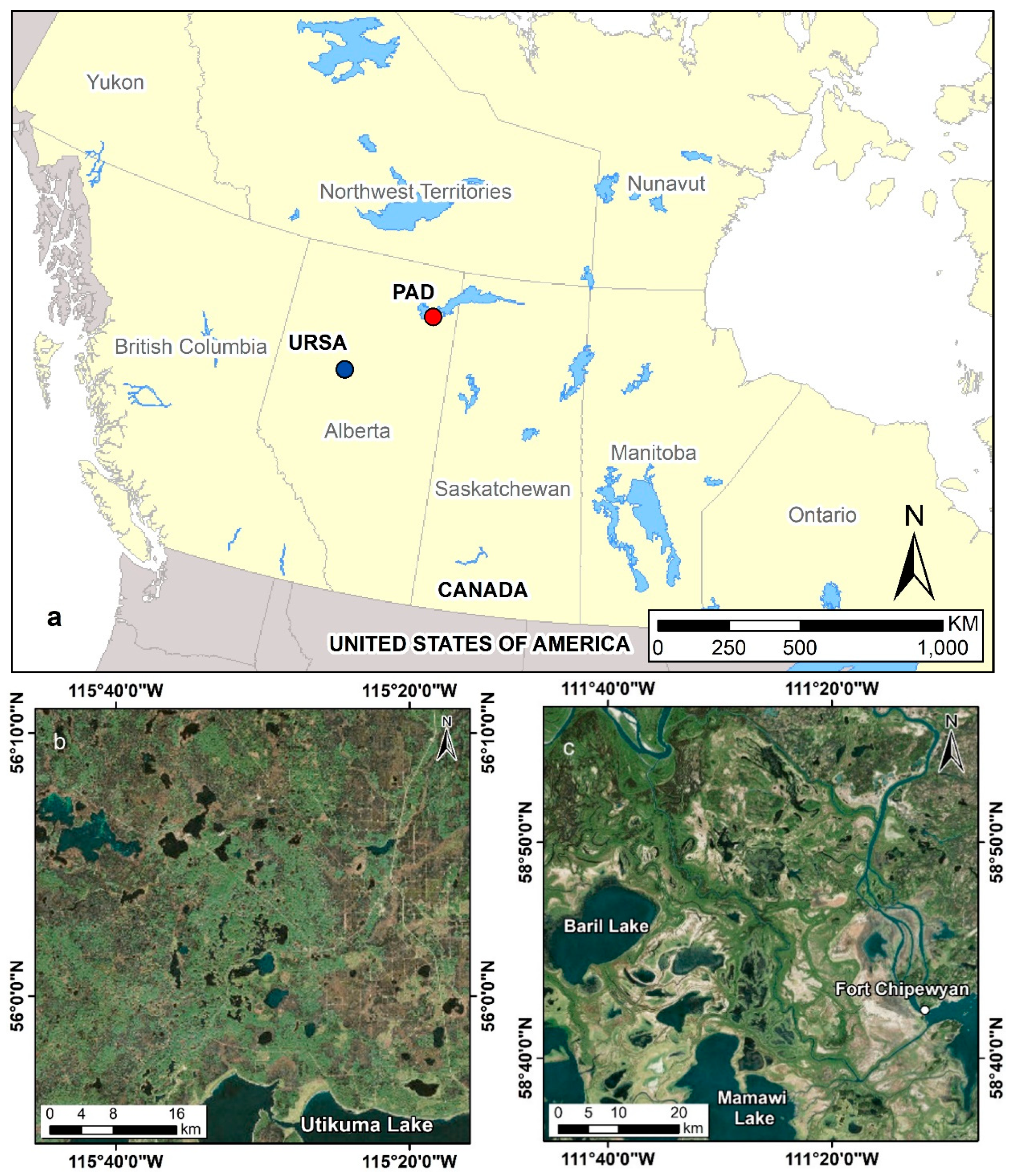
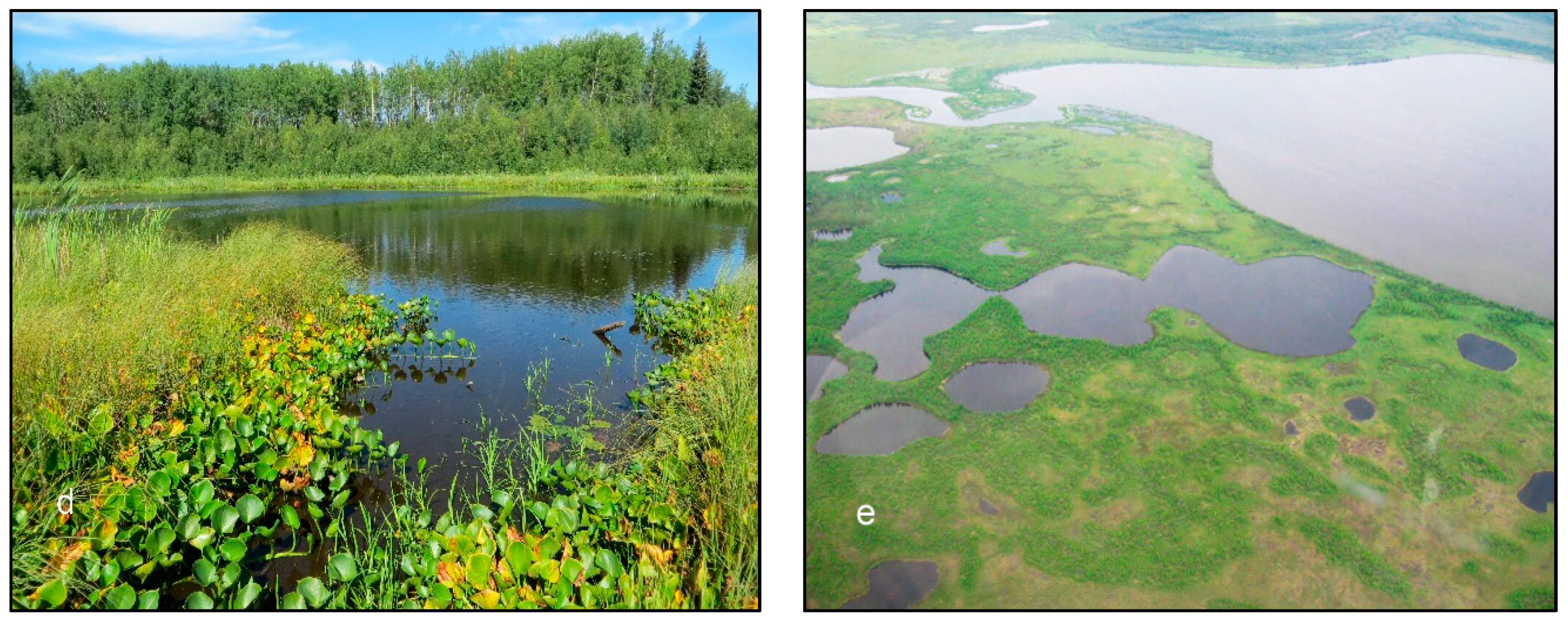
The research focuses on two subareas in Alberta (Figure 1a): a ~20 km × 20 km subset of the Utikuma Regional Study Area (URSA) region (Figure 1b), including only areas of heterogeneous wetland and till moraine uplands (excluding the clay plains region); and a ~25 km × 25 km area of the Peace-Athabasca Delta (PAD) (Figure 1c). The subarea found within the PAD was identified to test the applicability of remote sensing fusion classification conducted at URSA. It should be noted the shrub (Salix sp.) and graminoid dominant vegetation composition at PAD is different from that at URSA, which is more heavily treed and subject to less extreme surface water fluctuations. The difference in canopy density at each site is also an important consideration with respect to determining Lidar and SAR signal penetration and canopy height metrics.
1.2.1. Utikuma Regional Study Area
URSA is a boreal forest region located approximately 100 km north of Slave Lake in the Central Mixedwood Natural Subregion [20]. The URSA series of study sites covers an area of 1062 km2 surrounding Utikuma Lake [21], established in 1998 as a long-term monitoring site to quantify key hydrological processes associated with disturbance and regeneration, nutrient cycles, and hydro-ecological changes over time in a sub-humid environment. URSA moraine complexes are comprised of a heterogeneous mixture of locally topographic low-lying wetlands and peatlands separated by upland till moraine with predominantly Populus tremuloides across the northwest side of the ~60 km × 20 km transect. The southeast half of the transect is underlain by clay plains with large coverage of peatlands and greater development. Wetland ecosystems are predominantly comprised of shallow ponds with submergent macrophyte vegetation that may float on open water during summer [22]. Treed fens and bogs are found on poorly drained organic rich soils comprised of mainly black spruce (Picea mariana) and are commonly underlain with Sphagnum spp. mosses, fibric peat, grasses up to 0.5 m height, and gyttja hummocks and hollows [22].
1.2.2. Peace-Athabasca Delta
The Peace-Athabasca Delta (PAD) formed at the western end of Lake Athabasca after the retreat of the Laurentide ice sheet ~10,000 BP. Isostatic rebound and sedimentation by the major Peace, Athabasca, and Birch Rivers formed deltas approximately 1680, 1970, and 170 km2, respectively [23]. The deltas contain more than 1000 small basins (wetlands and lakes) with varying degrees of surface hydraulic connection to the main flow system, depending on location and elevation [24]. Three delta basin water level regimes are present within the PAD: (i) an open or active hydraulic connection with the main flow system; (ii) a restricted connection, such as a perched channel or levee entry, to an adjacent lake or river; and (iii) isolated farther inland. The water level fluctuation of the latter two types is independent of the main flow system, except when connected during high water events, and are referred to as perched basins.
Basins typically have low relief (<2 m, referred to as shallow open water wetlands, a standard Canadian national wetland class) with maximum depths ranging from 0.06 to 12.1 m (mean of 1.5 ± 1.4 m), and surface areas ranging from 0.1 to ~20 km2. Basins in the main portion of the delta are generally enclosed by narrow, abrupt levees that comprise a small fraction of the total area [25]. Topographic relief within the delta is low, and reconnection of abandoned channels and overland flow to inland basins occurs during overtopping of levees as a result of ice jams, large runoff, and/or the expansion of the central lakes beyond the shoreline. Vegetation cover is important in limiting surface runoff and influencing evaporation rates, while bedrock outcrop in the northeastern areas enhance surface runoff contribution to the ponded area [26,27].
2. Data and Methods
This study employed multi-temporal, multi-mode SAR (RADARSAT-2, single and quad polarization), Lidar, and optical (SPOT) data with similar acquisition dates. The data were acquired, and their intended purpose is summarized in Table 1.
2.1. Data
2.1.1. Airborne Lidar
Two airborne Lidar datasets were available at URSA. The first was acquired during August 2008 by Airborne Imaging Inc. (Calgary, AB, Canada) using a Teledyne Optech ALTM 3100. These data were acquired as part of Alberta’s provincial dataset. The second was a multispectral acquisition captured on 6 August 2016 by use of a Teledyne Optech Titan ALTM, geo-referenced using a locally situated global navigation satellite system (GNSS) unit. Both airborne Lidar datasets exhibit coincidence between all SAR acquisitions and field validation locations.
An additional multispectral Titan Lidar survey was flown over the PAD in August 2016 in a similar configuration as noted at URSA. No supplementary local geo-referencing information were acquired to support this dataset due to logistical and financial constraints.
2.1.2. Optical Data
SPOT-6 (Satellite Pour l’Observation de la Terre, Centre national d’études spatiales) multispectral optical imagery was acquired on 17 September 2015, which was cloud-free and delivered with an atmospheric correction applied. Each image captured 4 spectral bands, red (625–695 nm), green (530–590 nm), blue (450–524 nm), and near-infrared (NIR) (760–890 nm); at a 5 m × 5 m pixel resolution. Data were acquired near coincident days to SAR acquisitions, for validation purposes.
2.1.3. SAR
RADARSAT-2 images of URSA were acquired during 2015 and 2016 ice-off conditions in single polarization (HH) Wide Ultra-Fine U24W2 (incidence angle 46.3° to 48.2°) and U13W2 (incidence angle 38.7° to 41.2°) descending orbit, and Wide Fine-Quad FQ10/5W (incidence angle 22.5° to 26.0°) beam modes (Table 2). Wide Ultra-Fine U2W2 (incidence angle 29.6° to 33.0°) and Wide Fine-Quad (FQ10/5W) ascending orbit data were acquired over the PAD in 2014 and 2015 (Table 3). Wide Ultra Fine has a nominal resolution of 2.5 m × 2.5 m, and Wide-Fine Quad has a nominal resolution of 5 m × 5 m. Wide Ultra-Fine data were resampled to a 3 m resolution for consistency across all images.
Canopy penetration of the microwaves in the SAR system allows for mapping and classification of flooded vegetation due to enhanced backscatter from the double-bounce scattering mechanism [28,29]. This results in enhanced HH backscattering with less increase seen in VV, therefore, quad-polarized (HH, HV, VH, VV) datasets can be used to identify flooded vegetation using polarimetric decomposition techniques [29,30,31]. Steeper incidence angle gives better penetration into the canopy of flooded vegetation, but the steeper the angle, the more that the range is limited in Fine-Quad modes.
2.1.4. Ground Validation
A total of 6 wetlands within the study region were surveyed between 25 July and 4 August 2015. Positional information was acquired to determine surface water extent (i.e., location where water touches the edge of the pond) and riparian habitat boundary transects (i.e., location where the frequency of shrubs was less than ~1 shrub per 10 m radius). Cross-sectional transects were established, extending perpendicularly away from the water’s edge and upwards from the wetlands to adjacent upland, to reflect vegetation zones and changes in vegetation community composition where prominent vegetation species were identified [8]. Positions were occupied using a Topcon HiPer SR GNSS (Livermore, CA, USA) following standard kinematic survey techniques, and were differentially corrected to a static base station using precise point positioning (PPP), yielding centimeter accuracy.
In situ field data, collected within days of remote sensing data acquisitions, were utilized for spatially validating riparian vegetation species, composition, and open water extent over time, and/or pond/lake “hydroperiod”.
2.2. Methods
2.2.1. Airborne Lidar Processing
The 2016 Titan Lidar point cloud was pre-processed using Teledyne Optech’s Lidar Mapping Suite, where Terrascan (Terrasolid, Helsinki, Finland) and LAStools [32] were utilized for post-processing. The raw (pre-processed) point cloud was tiled to a 1 km grid, with a 20 m buffer to mitigate potential edge effects. Each tile was ground-classified and, subsequently, height normalized to calculate the height of each non-ground point above the identified ground surface. Non-ground points were classified as low, medium, and tall vegetation, in accordance with ASPRS 2011 guidelines [33]. Vegetation-classified points were interrogated using a 1 m search radius to determine the 99th percentile height (P99), where only points >2 m above the ground were considered, in order to negate contributions of understory vegetation; i.e., P99 is the height at which 99% of vegetation-classified points >2 m above the ground occur. These heights were rasterized to a 1 m grid to yield a canopy height model (CHM). The removal of understory vegetation by use of a minimum height cut-off is common practice in the analysis of Lidar data acquired over forest environments [34]. TerraScan (TerraSolid, Helsinki Finland) and Surfer (Golden Software, Golden, CO, USA) were employed to filter ground classified points and produce a 1 m × 1 m digital elevation model (DEM), created using inverse distance weighting (IDW) interpolation, with a 10 m search radius.
A common derivative from high resolution DEM data is topographic position index (TPI). TPI is a measure of the difference between the elevation value of a cell and the average elevation of nearby (neighboring) cells (within a defined radius) [34,35,36,37]. A positive value indicates higher elevation than its surrounding, whereas negative indicates it is lower. TPI results provide the means for estimating the probability of a wetland occurring in a certain area by separating locally high and low areas, assuming gravitational drainage of surface water. For example, the probability or landscape suitability of a wetland occurring in a topographic high (upland) may be low (for broad wetland areas and excluding local topographic depressions, e.g., forested swamps). A low TPI suggests high suitability for a wetland because surface water may flow towards depressions, therefore propagating the potential for wetland development.
At URSA, SAR and optical data were orthorectified to the 2008 Lidar DEM as it had more reliable geo-referencing information. Due to the lack of local geo-referencing information, Lidar data acquired at the PAD exhibited small positional discrepancies, which amassed themselves as relatively large errors due to the flat nature of the region. This resulted in the PAD Lidar dataset exhibiting too many uncertainties to produce a robust analysis with respect to inferring Lidar-based corrections; therefore, corrections with Lidar were only conducted over URSA.
2.2.2. Surface Water Extraction and Hydroperiod
SAR-derived surface water masks were created using an intensity (dB) thresholding technique developed by White et al. [14] using PCI Model Builder (PCI Geomatics). The methodology was modified to extract surface water using input threshold intensity/decibel (dB) range values [8]. Employed SAR filters (software specific naming) in the PCI Model Builder include FGAMMA (gamma maximum-a-posteriori (MAP)) adaptive filter to preserve edges, important for surface water extent analysis [37,38,39]; FAV (averaging mean filter) to reduce speckle [40]; and FMO (mode filtering of gray-level values) to further reduce noise of the SAR images [40]. SPOT 6 data were employed for the validation of SAR water masks (all bands were used to inform on water versus land pixels), where surface water was classified using K-means unsupervised classification [41,42,43]. Binary surface water extents (i.e., 0 as non-water, 1 as water) were produced in raster format for each available SAR acquisition using HH backscatter.
A measure of water permanence or hydroperiod throughout the growing season is determined using an “equals frequency” routine on the binary surface water rasters for each year, calculating the number of times a pixel is identified as water in the same geographic location. The output “pixel frequency” corresponds to the number of SAR images/months analyzed within each year. This is reclassified from frequency to hydroperiod classes based on Stewart and Kantrud [44] and Cowardin et al. [45]; where water present for 1–2 months represents “temporary” (S&K Class II), 3–4 months is “seasonal” (S&K Class III), and 5–6 months is “semi-permanent/permanent” (S&K Classes IV and V).
2.2.3. SAR Polarimetric Decompositions for Flooded Vegetation
The Freeman–Durden decomposition (FDD) [46] was used to create a three-channel composite raster that estimates the contribution of surface (water or rough surface), double-bounce (flooded), and volume (tall/forested vegetation) scattering response to the total backscatter from each pixel in an image. The double-bounce (flooded vegetation) band was isolated, and null values removed to represent only positive values in the double-bounce backscatter [31,40,47]. To remove speckle, a 5 × 5 boxcar filter (PCI Geomatica) was applied, based on local pixel averaging [29].
2.2.4. Topographic Position Index
TPI is scale dependent based on the topographic morphology of the land surface (defined by surface geology), therefore, the user needs to select parameters (e.g., window search radius) appropriate for the study area. In order to determine the optimal search radius, multiple iterations ranging from 50 m to 500 m were tested. Optimal radii was selected based on (1) the high resolution of the data, (2) topography criteria outlined by Jenness [48], and (3) circular moving polynomial windows based on the round shape and width of upland till moraines between the wetlands in the area [7]. The range of window sizes, selected to test TPI suitability to the landscape, were based on where the “normal” maximum occurs in the surface water. Isolated outlier wetland pixels from the hydroperiod analysis, located on plateaus, were manually identified and masked out, creating an adjusted hydroperiod from the TPI.
2.2.5. Decision-Based Workflow
A decision-based methodology was developed to derive wetland ecosystem attributes that expands upon an earlier method developed by Chasmer et al. [7,16] who based classification on topographic position and vegetation canopy attributes from Lidar and WorldView-2 spectra [16], and Lidar-based intensity and structure [7]. Variation in hydroperiod and impact on wetland aquatic transitional vegetation was performed using SAR. Water permanence and presence of flooded vegetation integration, in fusion with Lidar, follows findings by White et al. [40], and Brisco et al. [49] regarding the spatial distribution of wetland attributes. The decision-based methodology includes deriving SAR (single pol) water masks, associated hydroperiod classified according to Stewart and Kantrud [44], and the Government of Alberta [50], flooded vegetation from SAR (quad pol) FDD decomposition and, lastly, Lidar-derived topographic index and canopy cover attributes.
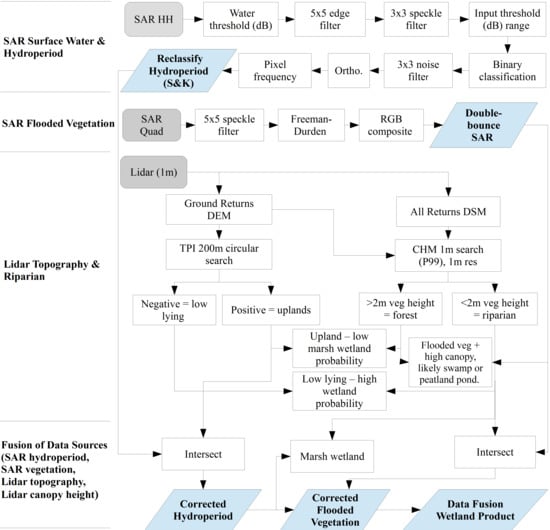
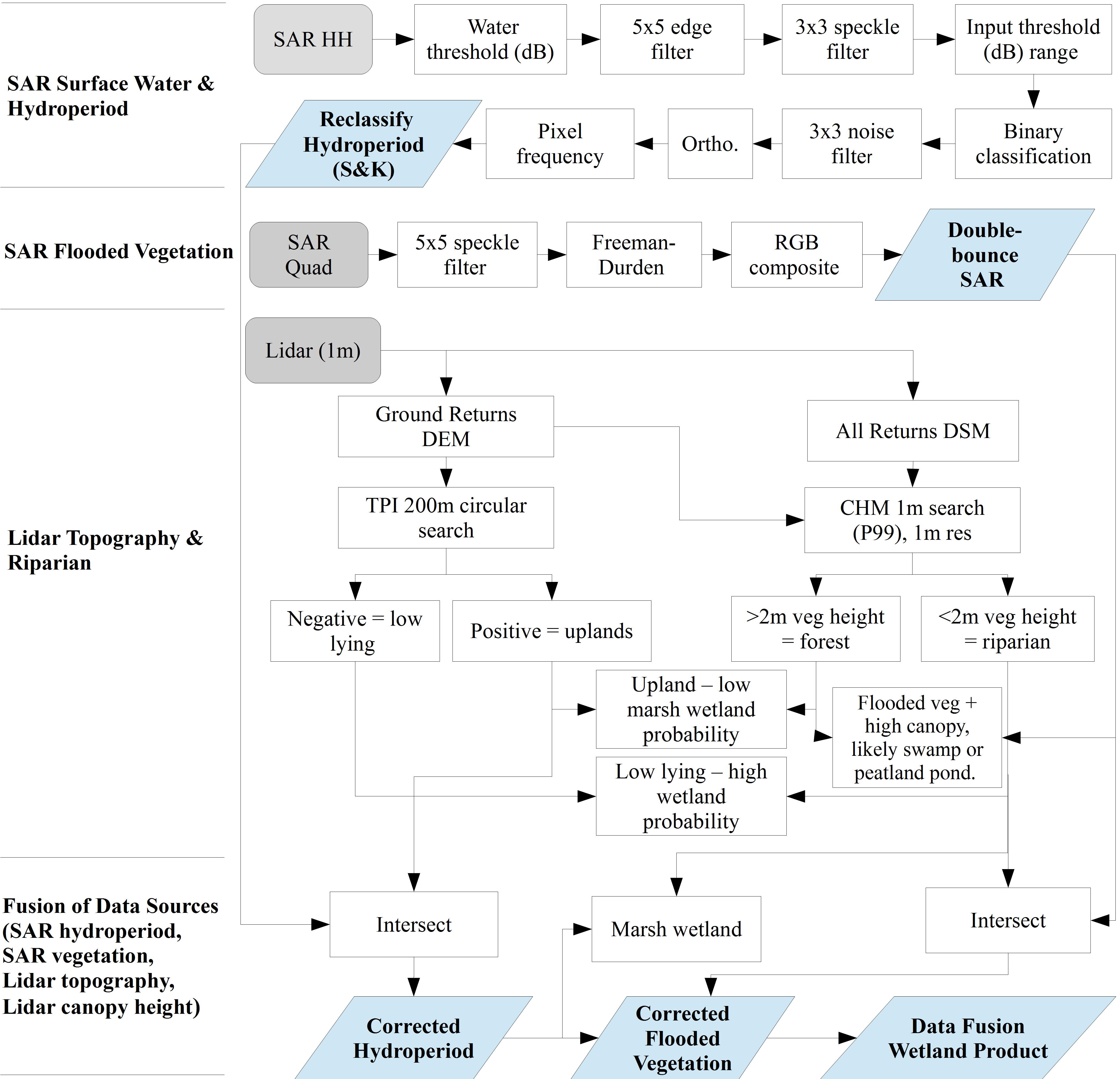
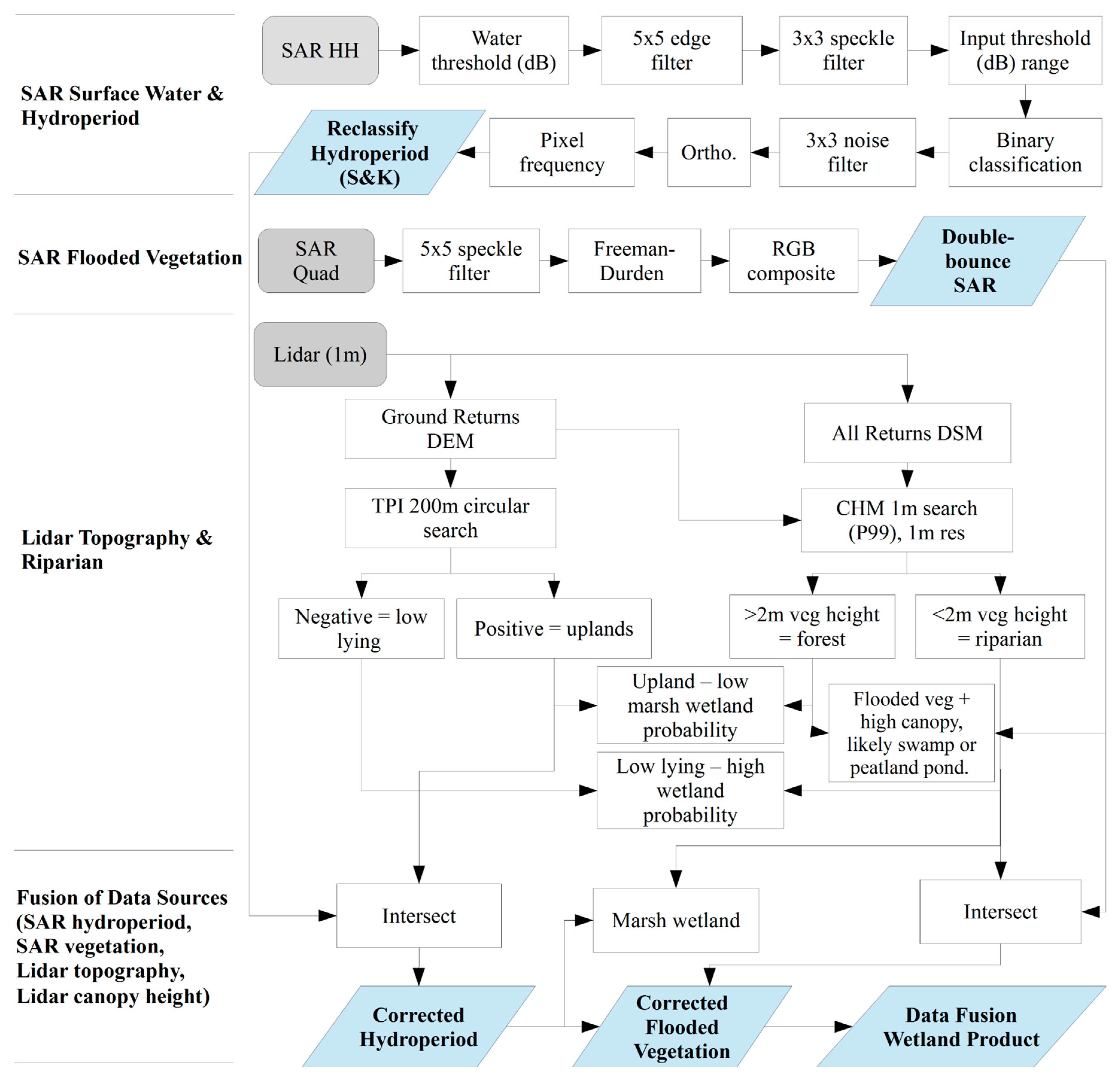
The methodology is broken into four different stages: (1) surface water extraction using intensity thresholding [14], and hydroperiod analysis [8]; (2) flooded vegetation using FDD decomposition [31]; (3) Lidar topographic attributes [7], and TPI [48]; and (4) data fusion of all attributes, enabling quality-controlled wetland ecosystem products. The combination of each dataset acts as a quality control measure, high resolution wetland classification system, and creates an integrated, dynamic wetland product with potential monitoring implications. Figure 2 provides an overall schematic of the methodology. A combination of statistical analyses (overall accuracy and kappa coefficient) and ground validation of the output classes were used to evaluate the best data fusion approach for mapping the riparian ecology and surface water extent of wetlands.
2.2.6. Validation of Remote Sensing Products
A direct comparison between field measure and remote sensing-derived water edge was conducted, with ecological boundaries identified based on the remote sensing data fusion product. The distance of these boundaries from the water’s edge were then compared to the ground validation data (i.e., distance from water’s edge). Standard statistical measures include coefficient of determination (R2), and root mean square error (RMSE).
3. Results
3.1. SAR Surface Water Masks
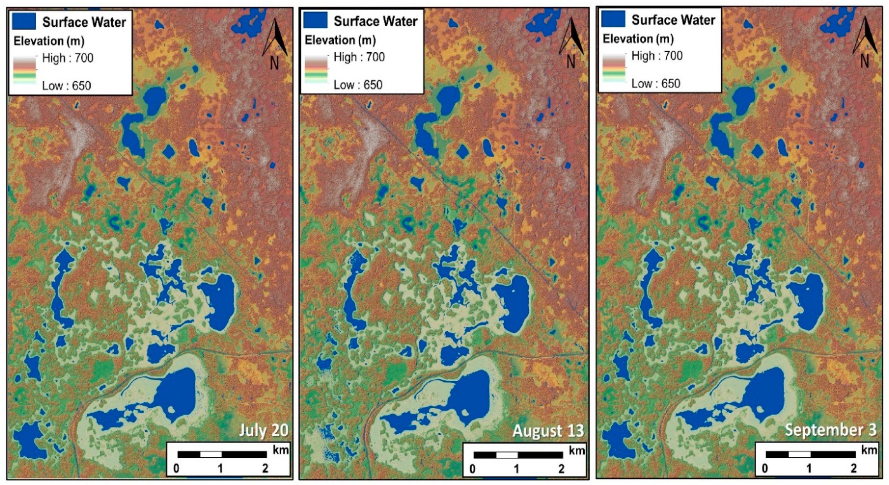
Intensity threshold (dB) surface water masks of boreal wetlands at the URSA region are shown in 2015 (Figure 3). The threshold range was similar in all images, with the average upper limit of −18 dB, and the lower limit of −30 dB. Decibel limits, ranging from −13 dB to −14 dB upper limit and −30 dB lower limit, were observed in the PAD, consistent with ranges found by White et al. [14].
Optical Validation
Optical satellite open water classification is a well-established method, and is therefore useful for validation with water masks derived from other sensors [51,52]. Peiman et al. (submitted to CJRS) [53] compared both ascending and descending SAR texture and intensity thresholding with a SPOT-6-derived mask from 17 September 2015 over the same study area. Despite slight temporal offset, overall accuracies were >90% (kappa = 0.8–0.95) (Table 4). Greater accuracy is expected without the temporal offset and with the removal of roadways and infrastructure (dark targets that appear as errors of commission in SAR data).
3.2. Surface Water Hydroperiod
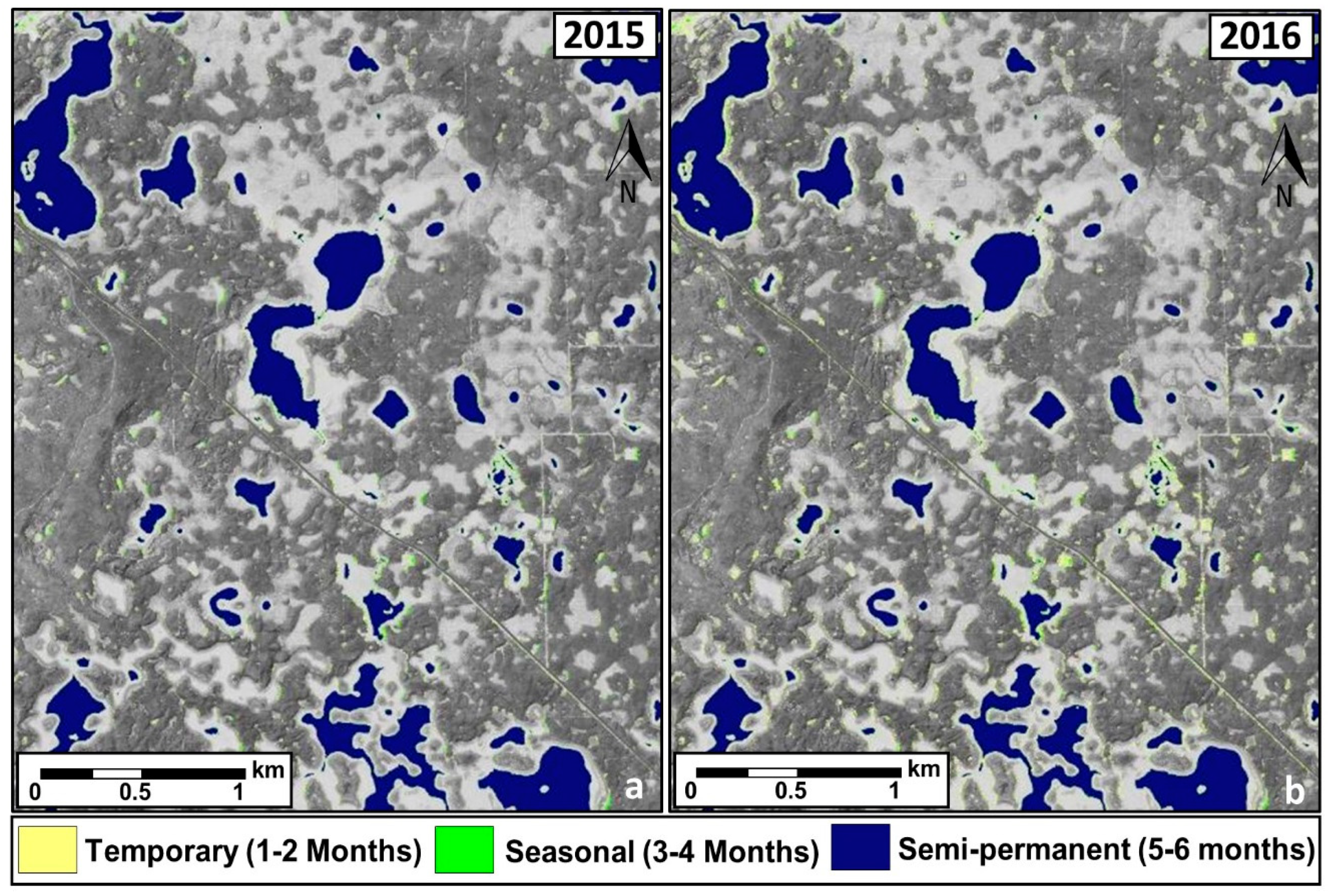
Surface water hydroperiod classes are presented for URSA in 2015 (Figure 4a) and 2016 (Figure 4b). Concordance results showing the proportion of pixels that are the same class in both 2015 and 2016 are detailed in Table 5. Overall similarity of hydroperiods on a pixel by pixel basis is 79%, attributed to the low similarity of temporary and seasonal hydroperiod compared to the very high similarity between semi-permanent/permanent. It should be noted there have been periods in the URSA area when many ponds dried out, but precipitation between 2015 and 2016 were about the same (2 years cu m departure from the long term mean between 0 and −120 mm). Additionally, wetting events in 2016 occurred in the fall of 2016, therefore, little difference would be expected.
Note that 2015 includes only six image acquisitions, compared to 14 acquisitions in 2016, where more scenes over the growing season increase the chance to capture additional temporary or seasonal surface water hydroperiod events. Therefore, it is expected that a comparable number of acquisitions from each year would change the comparative hydroperiod results.
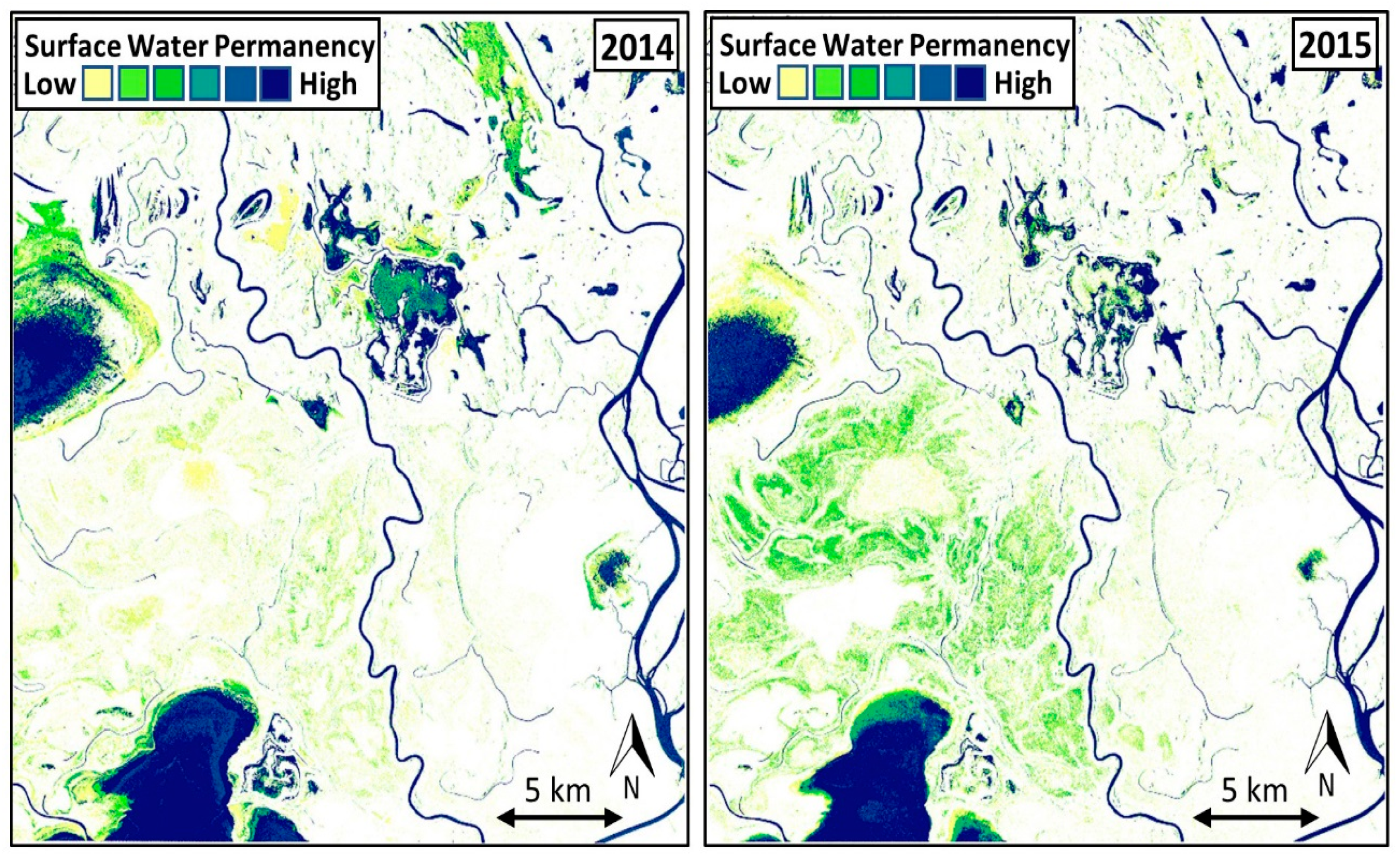
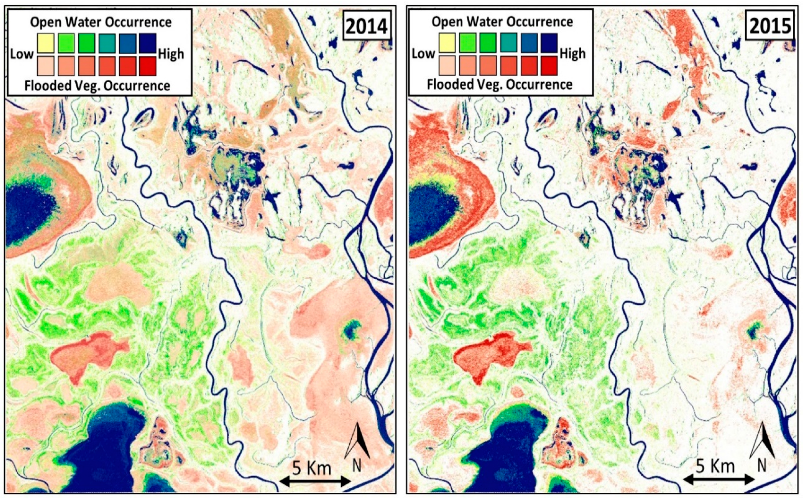
Hydroperiods in the PAD are less defined and have regions of significant change in surface water permanence (Figure 5). When comparing the difference between 2014 and 2015 hydroperiod along waterways, there are no notable areas where open surface water is changed. Some areas have greater permanence in 2015 (e.g., seen in green in the southwest quadrant of the AOI), whereas other areas have lower permanence (e.g., Baril lake located in the west of the AOI, and many wetland areas in the north of the AOI). Open water wetland and lake area permanence is far more variable. Approximately 18%–25% of the landscape is permanent in both years. The proportion of low permanence (yellow) is most changed along riparian areas of the larger water bodies, whereas the proportion of low to medium (green) is the most changed overall.
3.3. Flooded Vegetation
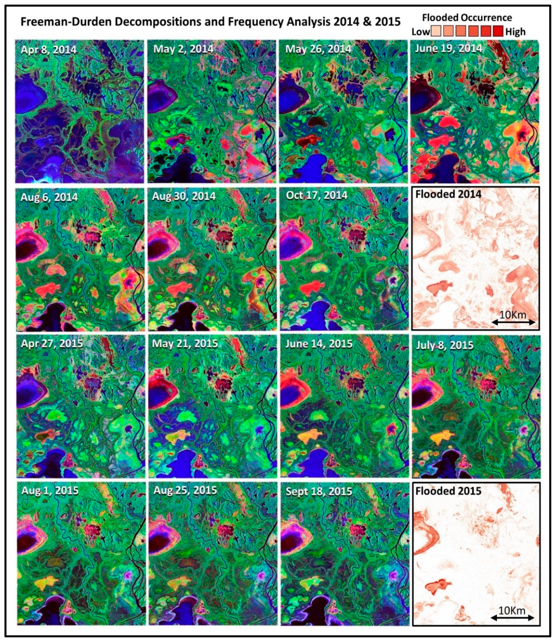
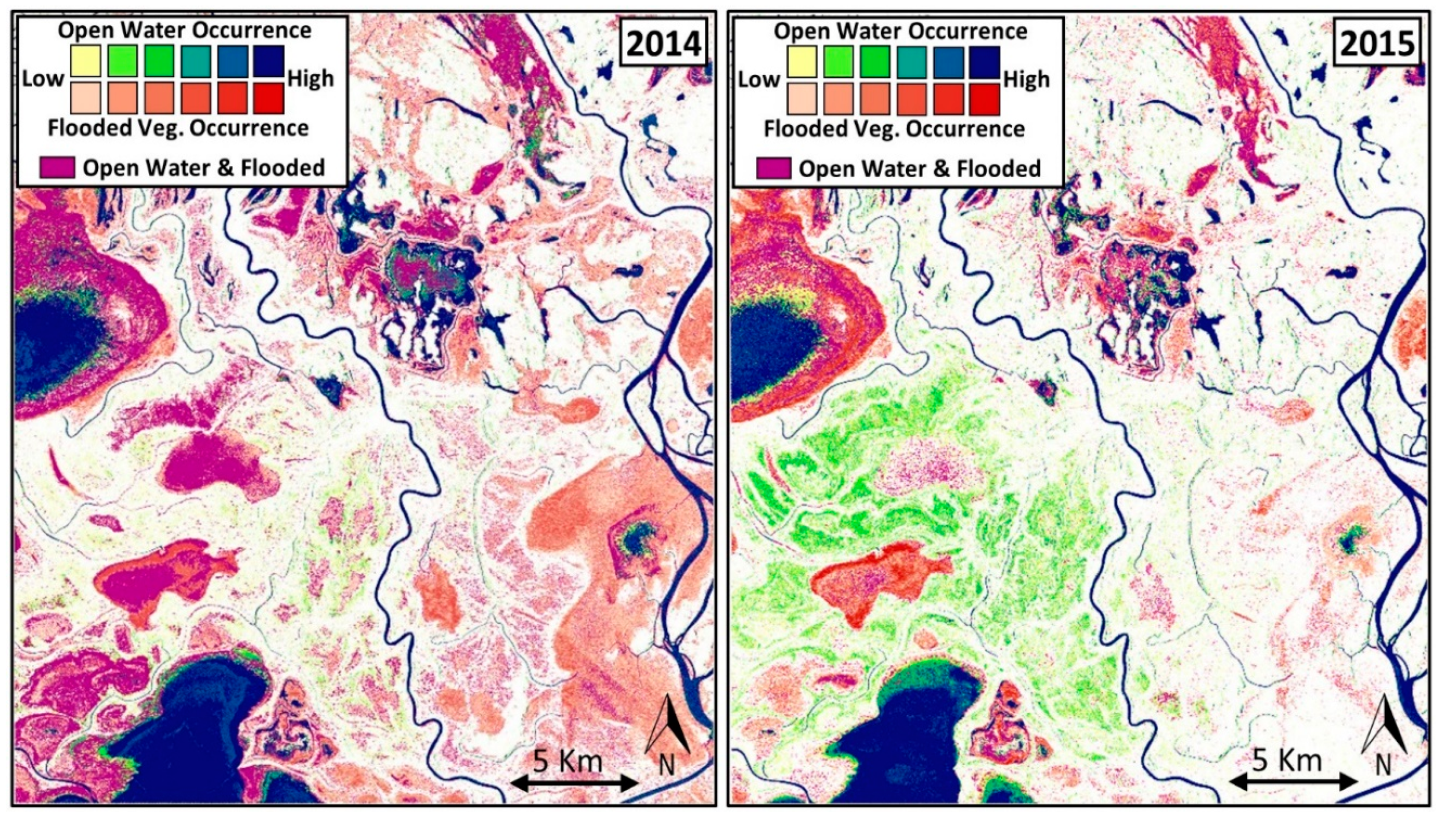
FDD results for each acquisition/month in the growing season and associated yearly flooded vegetation occurrence for the PAD, created using pixel frequency analysis, are shown in Figure 6. Ice is notably present in some areas of the waterbodies (bright purple-blue) in the early spring months (i.e., 8 April 2014), and fall months (i.e., 18 September 2015) around the margins of the wetlands. This may have an impact on the amount of true open surface water in the images but should not be removed from the analysis unless it is outside the growing season to reduce error associated with freezing and thawing of surface water that can change daily. Overall there is significantly more area of flooded vegetation in 2014, but the duration of flooded vegetation, notably around larger wetlands, is longer in 2015 (indicated by darker red areas).
Table 6 shows the difference in area between 2014 and 2015 at the PAD. The total flooded area is significantly different between the two years, most notably, the total hectares of temporarily flooded areas in 2014 (25,954 ha in 2014 compared to 10,263 ha in 2015). While there is significantly more flooded area in 2014, the proportion of more permanently flooded areas in 2015 (21%) is much higher than 2014 (11.2%).
3.4. Data Fusion Results
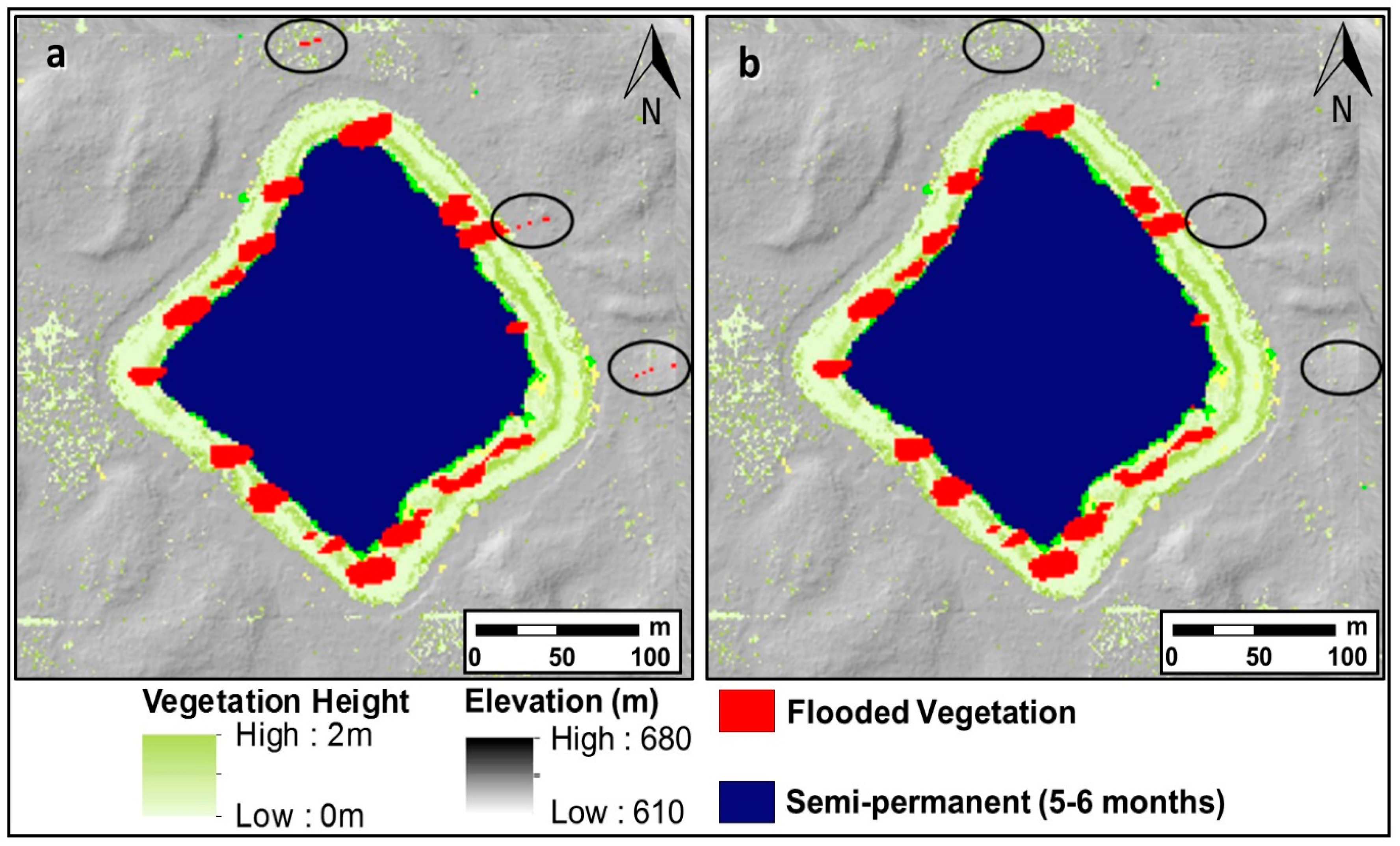
The results of the data fusion of both riparian vegetation and flooded vegetation from quad-polarized SAR are shown in Figure 7a. Flooded vegetation can be found in improbable areas such as roadways, and appear isolated from vegetation (<2 m) normally associated with flooded vegetation (circled in Figure 7a,b), but this effect is mitigated by intersecting the vegetation height layer from the CHM and the flooded vegetation mask, creating a corrected mask of flooded vegetation around wetlands (Figure 7b). This methodology also prohibits commission errors from areas of flooded vegetation where no vegetation height is recorded [54]. The combination of the riparian canopy height model derived from Lidar data and flooded vegetation double-bounce returns from SAR reduces commission errors from areas located in topographic uplands where positive values are found. This leaves only low areas where wetlands can form. Lastly, the corrected flooded vegetation and corrected hydroperiod products are overlain as complimentary products, creating a dynamic wetland attribute product.
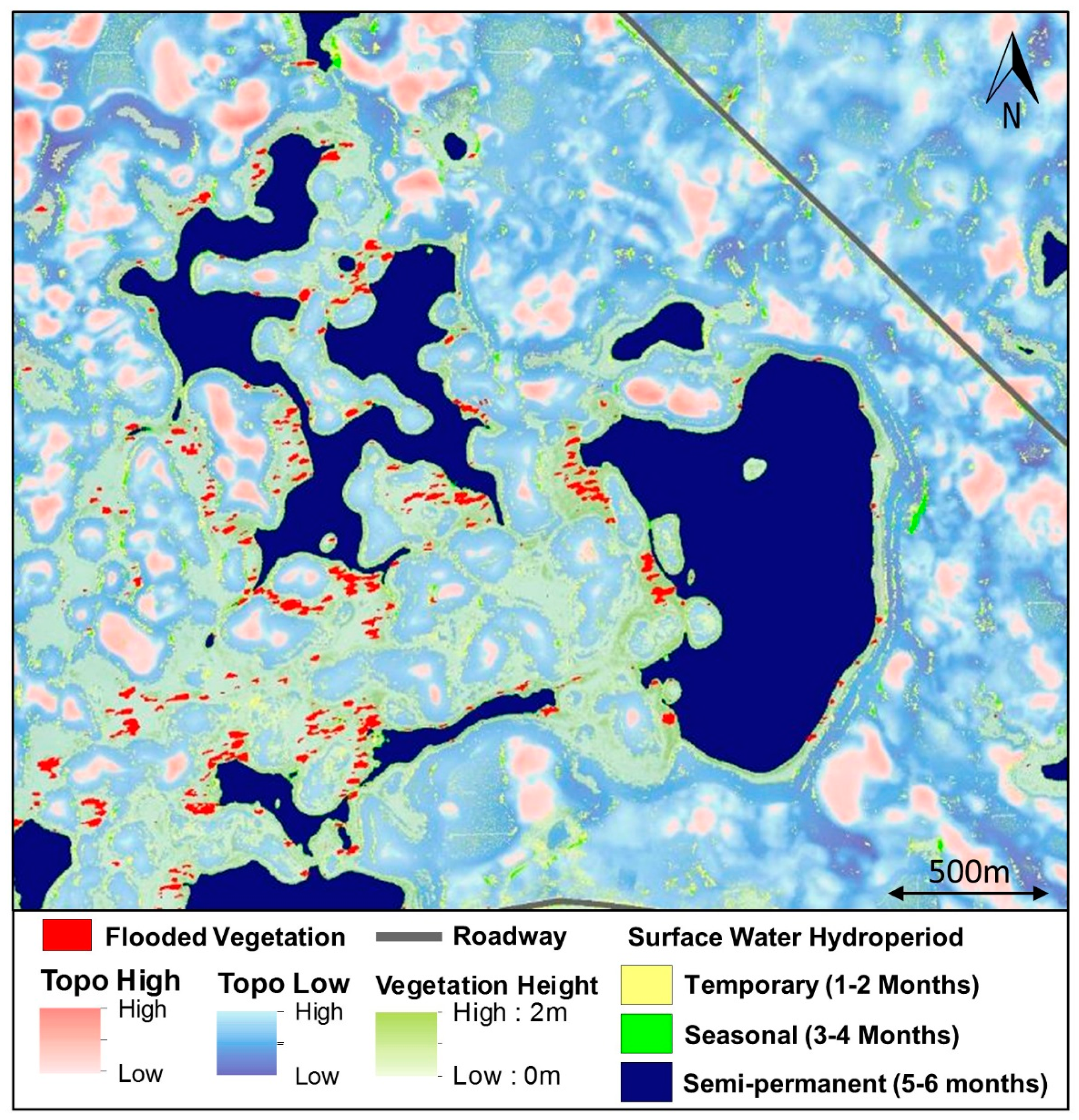
The comprehensive wetland attribute product is shown in Figure 8. Attributes include roadways derived from SPOT optical imagery, areas of high and low topography from the Lidar DEM topographic position index (where a search radius of 200 m was found to be most suitable for the landscape) indicating where wetlands are most and least likely to occur; vegetation height from Lidar CHM; flooded vegetation from quad-polarized SAR FDD; surface water hydroperiod from single polarization SAR data extracted from dB thresholding; and pixel frequency analysis in accordance with Stewart & Kantrud [44] surface water classification. Flooded vegetation is found to be located on the edges of the wetlands, either connected to the open surface water or adjacent, but still within the basin of the wetland. This is expected and typical of these wetlands, where a higher proportion of flooded vegetation, and one species in particular, Typha latifolia or common cattail, is commonly found within close proximity to larger ponds. These ponds are predominantly in areas that are part of larger hydrological complexes within or adjacent to peatlands.
In areas with cattail, little open water is observed in these areas of flooded vegetation, but flooded vegetation and topographic attributes suggest there is a high probability these areas are inundated, due to the saturated soil requirements of cattail. Flooded vegetation combined with hydroperiod is shown in Figure 9 in the PAD, and areas that have both open surface water and flooded vegetation for at least one month of the year are shown in dark pink in Figure 10, along with hydroperiod and flooded vegetation for each year for comparison.
3.5. Surface Water Extent and Riparian Vegetation Validation
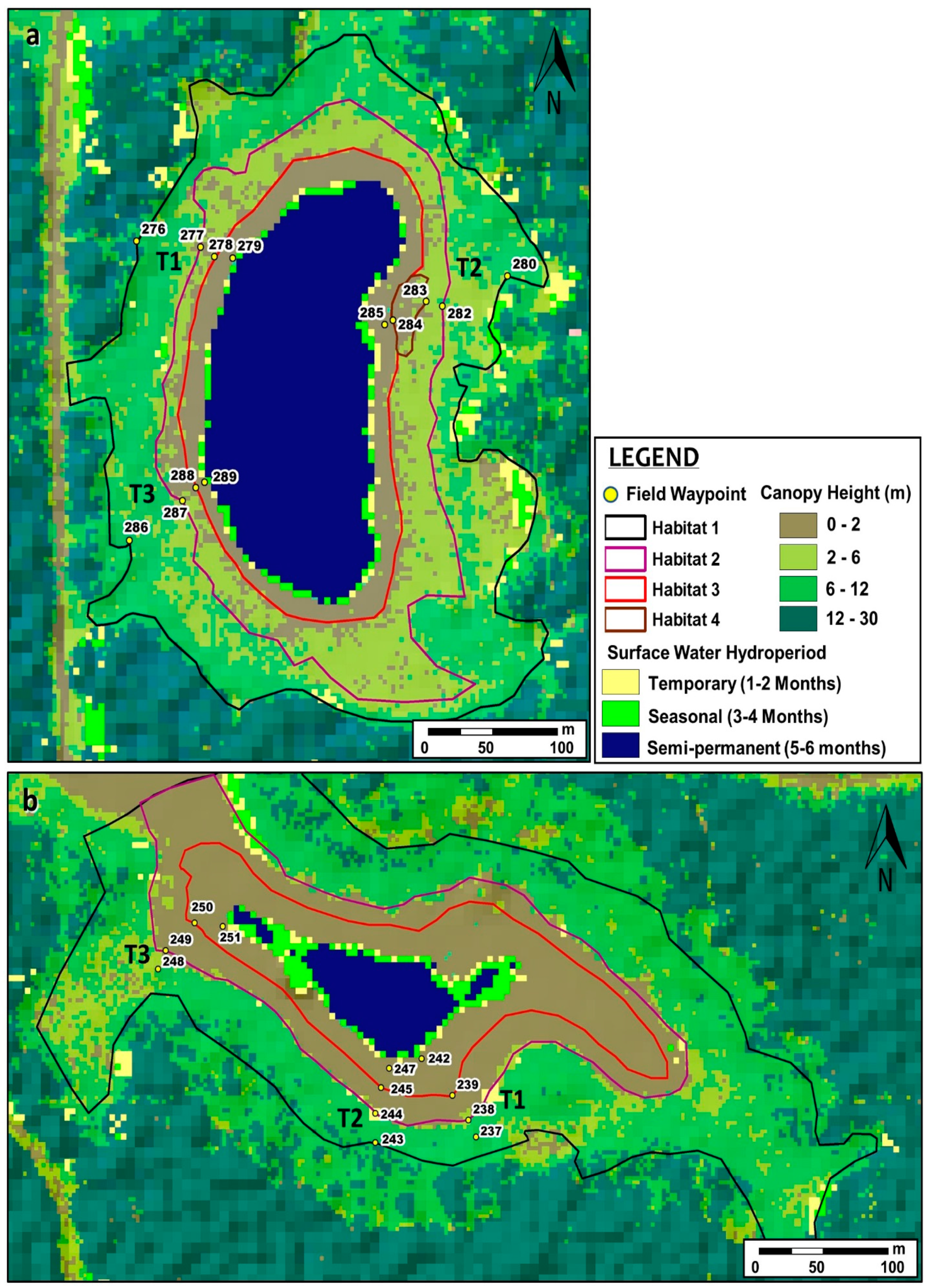
For clarity and display purposes, two of the six ponds are compared with field validation at URSA Pond 42 (Figure 11a) and Pond 48 (Figure 11b), as they are the most rigorously field validated and have an appropriate spatial scale for display purposes. Distinct riparian and upland vegetation zones were observed during 2015 field data collection. Transition zones are notably abrupt (vegetation zones are distinct) in most transects (Figure 11a,b), except for areas where there is encroachment of woody vegetation such as willow, alder, and birch, into grass- and forb-dominated wetland riparian areas, where patches of young woody vegetation have largely replaced tall grasses and sedge.
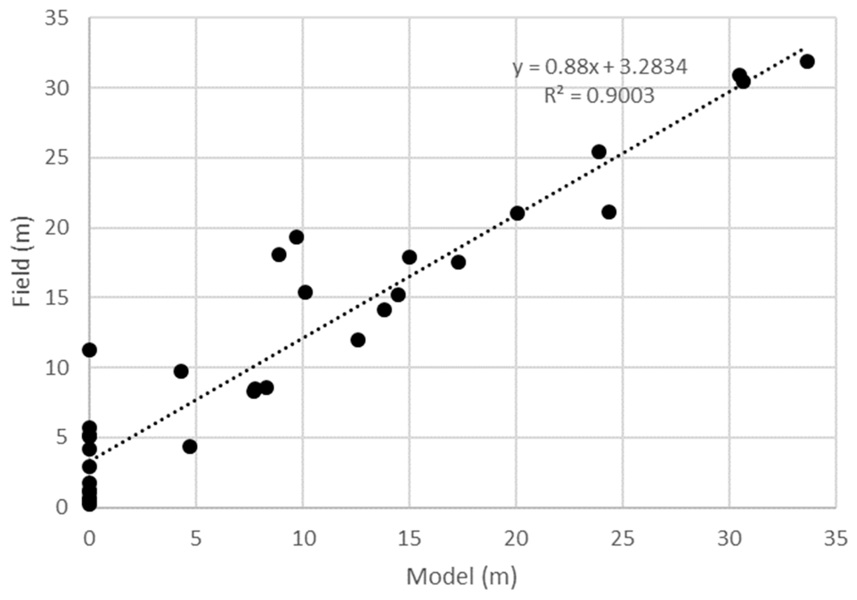
From the six wetlands surveyed, the RMSE of the riparian transects and water edge observed in field validation data and those predicted from the model was 4.6 m, with an R2 value of 0.90 (Figure 12).
Most of the error is attributed to some notable surface water extent discrepancies within fen ponds with mud flats separating surface water and riparian vegetation. Vegetation species composition by transect for Pond 42 and Pond 48 are detailed in Table 7 (Pond 42), and Table 8 (Pond 48). Species composition was found to be relatively consistent at each transect (T) for the wetlands, which can be divided into 3 distinct habitats (Hab.), with occasional pockets of unique vegetation communities (habitat 4, Figure 11a).
Vegetation communities observed at Pond 42 and Pond 48 were diverse at the time of data collection, with many wetland indicator species present (cattail, sedges), showing minimal to no anthropogenic disturbance. Vegetation growth was only observed to be limited in areas where woody vegetation, such as young willows and birch, was growing into the riparian area (e.g., Habitat 2 in all transects at Pond 48), potentially prohibiting succession of some riparian grasses.
4. Discussion
4.1. Subjectivity Associated with Manual Riparian Digitization
The results in Figure 11 and the associated accuracies in Figure 12 are accurate within ~10% of the area, but the manual classification shows some obvious discrepancies and associated subjectivity of the boundaries observed in the validation dataset and model. While optical data can be trained and classified to provide some measure of interpreted accuracy, the process is still largely determined by delineation conducted by the operator. Boundary delineation of vegetation and water extent in some wetlands are also subjective. Crasto et al. [55] discuss how criteria outlined by Jahn and Dunne [56] influence remote sensing feature detection, due to bias during digitization that is often influenced by experience and interpretations that are subjective [57]. All validation data were collected by the same individual in the field and areas were digitized by the same operator. Manual surveys of flooded vegetation boundaries were not conducted due to access and time limitations. Therefore, these areas could not be validated to the same degree as less saturated riparian areas, but the decomposition methodology has been well documented and studied for quality control in a variety of environments [31,46,58,59]. Any combination of uncertainties may contribute to discrepancies in the overall accuracy of the classification, and this highlights the importance of reliable ground validation data when working in logistically challenging regions.
4.2. Implications for Wetland Classification
While many studies focus on mapping known permanent waterbodies, this study differs by utilizing high spatial and temporal resolution information to create dynamic surface water and riparian vegetation thematic maps. Data availability is the most important aspect when attempting to characterize non-permanent wetlands, requiring increased temporal resolution and field measurements that represent the natural ranges in hydrological conditions. The results of this study suggest that these criteria can be met by products of the decision-based methodology presented (Figure 8, Figure 9 and Figure 10).
The methodology presented should also be useful for the identification of marsh and swamp wetlands with associated open water areas, while wet areas within fens can be identified using laser return intensity and other spectral indices that are related to the absorption of electromagnetic wavelengths by water [7,16], especially within peatland (treed fen/bog) environments. For example, Boolean statements can be implemented to determine if an area is a swamp: e.g., (1) “if” trees are present and topography is low-lying (TPI) then high potential for a swamp; (2) “if” the surface water level is above the DEM then high potential for a swamp; (3) “if” no open water is present and flooded vegetation is present then more likely a swamp or fen. However, “if” statements require calibration, which is locally dependent. Absence of these statements in the current methodology is a limitation, but they should be explored and integrated in further studies to provide a more complete classification system for boreal wetlands. Future work may also investigate scattering returns from volume scattering that intersect with areas of surface water at certain times of the year to provide an indication of species type. For example, some emergent hydrophytic vegetation, such as cattail and bulrush, tend to grow later in the growing season (July–August) in areas where soil was saturated in earlier months. Therefore, identifying the areas with transition from open water to double-bounce flooded vegetation and, lastly, volume scattering, could be an excellent indicator of these larger, slow growing species.
4.3. Data Limitations and Potential Sources of Error
A limitation of the study relates to temporal image frequency of both SAR and Lidar data. Increased temporal resolution will better represent short-term variations. The Canadian C-Band RADARSAT Constellation Mission (RCM), expected to launch in February 2019, will offer advanced capabilities for monitoring surface water with high spatial resolution modes such as Spotlight, providing enhanced monitoring of smaller wetlands [60]. As the provincial Lidar database and coverage in Alberta expands and is updated, there is a growing opportunity to integrate temporal Lidar datasets into wetland monitoring and enhance the understanding of precipitation variation influences, anthropogenic and climate change on surface water and wetland vegetation change.
Working over broad regions and in relatively remote areas like the URSA region makes it logistically difficult to collect ground validation across all wetland environments. Since classifiers or ranges for SAR-derived surface water masks are variable between images and acquisition, there is a need to calibrate the intensity threshold (dB) for each image to consistently extract all true open water returns from an image [14], as well as instrument calibration and ground conditions [61].
Another limitation of this approach is found in the fine resolution used in the large spatial area. Subtle changes in riparian vegetation on the order of <2 m are difficult to extract with certainty, due to homogeneity of many of the riparian vegetation communities. While it is easy to determine high and low topographical areas, and high, medium, and low vegetation canopy, it is difficult to discriminate between species. For example, while it may be important to examine species encroachment or succession, the difference between a patch of 2 m tall willow trees and 2 m tall birch trees is challenging due to similarities in structure, therefore, it was found to be more convenient to group these similar canopy environments. This is detailed in Figure 7a,b and Figure 8, where both elevation and canopy height are somewhat ambiguous, likely as a result of the general flatness of topography and sporadic woody vegetation regeneration in clearings and meadows.
Shadow effects in the SAR ascending and descending images can cause classification errors along some forested boundaries, but quality control data were not available within this study, so the extent (if at all) of such shadow-induced errors in low-lying riparian areas of the URSA study area is unknown. See Kropatsch [62] for details and methods to reduce error associated with shadowing.
When using SAR to derive surface water compared to other sensors, occasional omission of surface water bodies that are narrow or have mixed pixels (such as watercourses and fen pond boundaries), has been documented in shallow riparian areas [13]. This may be a potential source of error in many boreal wetlands, where these boundary areas are mostly classified as land due to the unique scattering properties. Hydrological connectivity of wetlands is of key interest to hydrologists and multi-temporal SAR imagery may provide an indication of hydrological connectivity due to periodic saturation and the growth of certain species. This may not be topographically related as the water can move underground in peat. It has implications for contaminant transport, downstream flooding, and ecosystem change. Surface water modeling would also be enhanced by delineating water extent and elevation from Lidar, which can also provide further high-resolution comparative data to both optical and SAR-derived surface water masks, adding utility to the wetland classification [55,63].
5. Conclusions
The presented methodology offers a new time series-based boreal wetland classification approach using data fusion of multiple remote sensing data sources, based on hydroperiod, topography and vegetation attributes. The results of this study indicate water mask frequency analysis can be used to determine hydroperiod and permanence in boreal environments, similarly to prairie environments, with overall accuracies of 93% to 97.2% and kappa values of 0.8–0.9% when compared to optical data. Concordance results comparing semi-permanent/permanent hydroperiod between 2015 and 2016 was found to be 98.3% correlated, suggesting there is very little change in open water extent in these wetlands between the two years. A longer time series would need to be used to determine if this is a consistent relationship given the climate cycles [20]. Regression analysis of field and model riparian and surface water extents from six wetlands also yielded high accuracies (R2 = 0.9), suggesting the decision-based methodology could be applied to similar open water boreal wetlands with some certainty. The time-intensive and potential limiting factor of the methodology is the expertise required in data preparation for multiple types of data (Lidar, SAR, optical). However, once the data preparation and foundation for data fusion has been conducted, additional data can readily be integrated and processed in the workflow. While there are limitations associated with data availability and frequency, the strength of the study is the ability to construct and examine meaningful comprehensive wetland characterization products conforming to provincial guidelines set forth by the American Wetland Classification System and the Canadian Wetland Classification System.
Future research using a logic-based decision-based methodology would benefit from identifying additional topographic and vegetative attributes at a higher resolution to increase class reliability. SAR and optical data to compliment Lidar data describing riparian vegetation communities would further enhance the hydroperiod analysis for a more comprehensive wetland classification and monitoring framework. This framework could be largely automated through machine learning algorithms and would provide a platform for land use permitting, reclamation monitoring, and wetland regulation in remote boreal regions of Alberta.
Author Contributions
Conceptualization, J.M., B.B., C.H.; methodology J.M., C.H., L.C.; software: C.H.; validation, J.M.; formal analysis, J.M.; investigation, K.D.; resources, B.B., C.H.; data curation, J.M., B.B.; writing—original draft preparation, J.M., C.H.; writing—review and editing, J.M, C.H., B.B., L.C.; visualization, J.M.; supervision, C.H., B.B., D.C., K.D.; project administration, B.B., C.H.; funding acquisition, C.H., B.B.
Funding
Hopkinson acknowledges: Alberta Economic Development and Trade, Canada Centre for Mapping and Earth Observation (CCMEO); Canada Foundation for Innovation and the Campus Alberta Innovates Program (project 32436); Project-related lab personnel, research and data funding to support SAR time series wetland classification and wetland ecosystem monitoring from Government of Alberta (Economic Development and Trade, Environment and Parks), Alberta Sustainable Resource Development (now Alberta Environment and Parks); and Discovery Grant funding from the Natural Sciences and Engineering Research Council (RGPIN-2017-04362). Funding is also provided by the Government of Alberta Oil Sands Monitoring Program, Wetland Ecosystem Monitoring; and Natural Resources Canada, Canada Centre for Mapping and Earth Observation (CCMEO).
Acknowledgments
We acknowledge support and field assistance from Craig Mahoney, Maxim Okhrimenko and Reed Parsons, Stephanie Connor. RADARSAT-2 imagery was obtained and licensed from the Canada Centre for Mapping and Earth Observation, Earth Sciences Sector (Ottawa) and MDA with the assistance of Kevin Murnhagen (CCRS). Archive Lidar data were provided by Alberta Environment and Parks, while new Lidar were obtained via support from Teledyne Optech Inc., Airborne Imaging Inc. Kalus Aviation Inc. Accommodations at the URSA camp.
Conflicts of Interest
The authors declare no conflict of interest.
References
- National Wetlands Working Group. Wetlands of Canada; Ecological Land Classification Series, No. 24; Environment Canada and Polyscience Publications Inc.: Ottawa, ON, Canada, 1988; p. 452.
- Komers, P.E.; Stanojevic, Z. Rates of disturbance vary by data resolution: Implications for conservation schedules using the Alberta Boreal Forest as a case study. Glob. Chang. Biol. 2013, 19, 2916–2928. [Google Scholar] [CrossRef] [PubMed]
- Devito, K.J.; Mendoza, C.; Petorone, R.M.; Kettridge, N.; Waddington, J. Utikuma Region Study Area (URSA)—Part 1: Hydrogeological and ecohydrological studies (HEAD). For. Chron. 2016, 92, 57–61. [Google Scholar] [CrossRef]
- Stow, D.A.; Hope, A.; McGuire, D.; Verbyla, D.; Gamon, J.; Huemmrich, F.; Houston, S.; Racine, C.; Sturm, M.; Tape, K. Remote sensing of vegetation and land-cover change in Arctic tundra ecosystems. Remote Sens. Environ. 2004, 89, 281–308. [Google Scholar] [CrossRef]
- Riordan, B.; Verbyla, D.; McGuire, A.D. Shrinking ponds in subarctic Alaska based on 1950–2002 remotely sensed images. J. Geophys. Res. 2006, 111, G04002. [Google Scholar] [CrossRef]
- Kettridge, N.; Waddington, J.M. Towards quantifying the negative feedback regulation of peatland evaporation to drought. Hydrol. Process. 2013, 28, 3728–3740. [Google Scholar] [CrossRef]
- Chasmer, L.; Hopkinson, C.; Montgomery, J.; Petrone, R. A physically based terrain morphology and vegetation structural classification for wetlands of the boreal plains, Alberta, Canada. Can. J. Remote Sens. 2016, 42, 521–540. [Google Scholar] [CrossRef]
- Montgomery, J.; Hopkinson, C.; Brisco, B.; Patterson, S.; Rood, S. Wetland hydroperiod classification in the western prairies using multi-temporal synthetic aperture radar. Hydrol. Process. 2018, 31, 1476–1490. [Google Scholar] [CrossRef]
- Houhoulis, P.F.; Michener, W. Detecting wetland change: A rule-based approach using NWI and SPOT-XS data. Photogramm. Eng. Remote Sens. 2000, 66, 205–211. [Google Scholar]
- Davranche, A.; Lefebvre, G.; Poulin, B. Wetland monitoring using classification trees and SPOT-5 seasonal time series. Remote Sens. Environ. 2000, 114, 552–562. [Google Scholar] [CrossRef]
- Wang, K.; Franklin, S.; Guo, X.; He, Y.; McDermid, G. Problems in remote sensing of landscapes and habitats. Prog. Phys. Geogr. 2009, 33, 1–22. [Google Scholar] [CrossRef]
- Brisco, B.; Short, N.; van der Sanden, J.; Landry, R.; Raymond, D. A semi-automated tool for surface water mapping with Radarsat-1. Can. J. Remote Sens. 2009, 35, 336–344. [Google Scholar] [CrossRef]
- Santoro, M.; Wegmüller, U. Multi-temporal synthetic aperture radar metrics applied to map open water bodies. IEEE J. Sel. Top. Appl. Earth Obs. Remote Sens. 2014, 7, 3225–3238. [Google Scholar] [CrossRef]
- White, L.; Brisco, B.; Pregitzer, M.; Tedford, B.; Boychuck, L. RADARSAT-2 beam mode selection for surface water and flooded vegetation mapping. Can. J. Remote Sens. 2014, 40, 135–151. [Google Scholar]
- Wang, J.; Shang, J.; Brisco, B.; Brown, R. Comparison of multidate radar and multispectral optical satellite data for wetland detection in the Great Lakes Region. In Proceedings of the International Symposium, Geomatics in the Era of RADARSAT (GER’97), Ottawa, ON, Canada, 25–30 May 1997. [Google Scholar]
- Chasmer, L.; Hopkinson, C.; Quinton, W.; Veness, T.; Baltzer, J. A decision-tree classification for low-lying complex land cover types within the zone of discontinuous permafrost. Remote Sens. Environ. 2014, 143, 73–84. [Google Scholar] [CrossRef]
- Ameli, A.; Creed, I. Quantifying hydrologic connectivity of wetlands to surface water systems. Hydrol. Earth Syst. Sci. 2017, 21, 1791–1808. [Google Scholar] [CrossRef]
- Irwin, K.; Beaulne, D.; Braun, A.; Fotopoulos, G. Fusion of SAR, optical and airborne lidar for surface water detection. Remote Sens. 2017, 9, 890. [Google Scholar] [CrossRef]
- Millard, L.; Richardson, M. Wetland mapping with Lidar derivatives, SAR polarimentric decompositions, and Lidar/SAR fusion using a random forest classifier. Can. J. Remote Sens. 2013, 39, 290–307. [Google Scholar] [CrossRef]
- Devito, K.; Mendoza, C.; Qualizza, C. Conceptualizing Water Movement in the Boreal Plains. Implications for Watershed Reconstruction; Synthesis Report; The Canadian Oil Sands Network for Research and Development, Environmental and Reclamation Research Group: Edmonton, AB, Canada, 2012; p. 164. [Google Scholar] [CrossRef]
- Devito, K.J.; Creed, I.; Gan, T.; Mendoza, C.; Petrone, R.; Silins, U.; Smerdon, B. A framework for broad scale classification of hydrologic response units on the Boreal Plain: Is topography the last thing to consider? Hydrol. Process. 2005, 19, 1705–1714. [Google Scholar] [CrossRef]
- Downing, D.J.; Pettapiece, W.W.; Natural Regions Committee. Natural Regions and Subregions of Alberta; Pub #T/852; Government of Alberta: Edmonton, AB, Canada, 2006.
- Peace-Athabasca Project Group. The Peace-Athabasca Delta Project Technical Report (1 Volume) + Technical Appendices (3 Volumes): Technical Report—A Report on Low Water Levels in Lake Athabasca and Their Effects on the Peace-Athabasca Delta. V.1 Appendices—Hydrologic Investigations; V.2 Appendices—Ecological Investigations; V.3 Appendices—Supporting Studies; Peace-Athabasca Delta Project Group: Delta, BC, Canada, 1973. [Google Scholar]
- Jaques, D.R. Topographic Mapping and Drying Trends in the Peace-Athabasca Delta, Alberta Using LANDSAT MSS Imagery; Report for Wood Buffalo National Park; Ecostat Geobotanical Surveys Inc.: Fort Smith, NT, Canada, 1989; p. 36. [Google Scholar]
- Wolfe, B.B.; Hall, R.; Last, W.M.; Edwards, T.W.D.; English, M.; Karst-Riddoch, T.L.; Paterson, A.M.; Palmini, R. Reconstruction of Multi-Century Flood Histories from Oxbox Lake Sediments, Peace Athabasca Delta, Alberta, Canada. Hydrol Proces. 2006, 20, 4131–4153. [Google Scholar] [CrossRef]
- Peters, D.L.; Prowse, T.D.; Marsh, P.; Lafleur, P.M.; Buttle, J.M. Persistence of water within Perched Basins of the Peace-Athabasca Delta, Northern Canada. Wetl. Ecol. Manag. 2006, 14, 221–243. [Google Scholar] [CrossRef]
- Peters, D.L.; Prowse, T.D.; Pietroniro, A.; Leconte, R. Flood hydrology of the Peace Athabasca Delta, northern Canada. Hydrol. Process. 2006, 20, 4073–4096. [Google Scholar] [CrossRef]
- Pope, K.O.; Rejmankova, E.; Paris, J.F.; Woodruff, R. Detecting seasonal flooding cycles in marshes of the Yucatan Peninsula with SIR-C polarimetric radar imagery. Remote Sens. Environ. 1997, 59, 157–166. [Google Scholar] [CrossRef]
- Townsend, P.A. Relationship between forest structure and the detection of flood inundation in forested wetlands using C-band SAR. Int. J. Remote Sens. 2002, 23, 443–460. [Google Scholar] [CrossRef]
- Brisco, B.; Kapfer, M.; Hirose, T.; Tedford, B.; Liu, J. Evaluation of C-band polarisation diversity and polarimetrey for wetland mapping. Can. J. Remote Sens. 2011, 37, 82–92. [Google Scholar] [CrossRef]
- Brisco, B. Mapping and monitoring surface water and wetlands with synthetic aperture radar. In Remote Sensing of Wetlands, Applications and Advances; Tiner, R.W., Lang, M.W., Klemas, V.V., Eds.; CRC Press: Boca Raton, FL, USA, 2015; Chapter 6; pp. 119–136. [Google Scholar]
- Isenburg, M. LAStools—Efficient LiDAR Processing Software (Version 141017, Academic). 2017. Available online: http://rapidlasso.com/LAStools (accessed on 11 May 2018).
- American Society for Photogrammetry and Remote Sensing (ASPRS). LAS Specification, Version 1.4-R6. 2011. Available online: www.asprs.org (accessed on 19 September 2018).
- Mahoney, C.; Hall, R.; Hopkinson, C.; Filiatrault, M.; Beaudoin, A.; Chen, Q. A forest attribute mapping framework: a pilot study in a northern boreal forest, Northwest Territories, Canada. Remote Sens. 2018, 10, 1338. [Google Scholar] [CrossRef]
- Guisan, A.; Weiss, S.B.; Weiss, A.D. GLM versus CCA spatial modeling of plant species distribution. Kluwer Academic Publishers. Plant Ecol. 1999, 143, 107–122. [Google Scholar] [CrossRef]
- Jones, K.B.; Heggem, D.T.; Wade, T.G.; Neale, A.C.; Ebert, D.; Nash, M.S.; Mehaffey, M.H.; Goodman, I.A.; Hermann, K.A.; Selle, A.R.; et al. Assessing landscape conditions relative to water resources in the western United States: A strategic approach. Environ. Monit. Assess. 2000, 64, 227–245. [Google Scholar] [CrossRef]
- Weiss, A. Topographic Position and Landforms Analysis. Presented at ESRI User Conference, San Diego, CA, USA, 9–13 July 2001. [Google Scholar]
- Toutin, T. Corrigendum to the paper State-of-the-art of geometric correction of remote sensing data: A data fusion perspective. Int. J. Image Data Fusion 2011, 2, 283–286. [Google Scholar] [CrossRef]
- Zhang, F.; Xie, C.; Li, K.; Xu, M.; Wang, X.; Xia, Z. Forest and deforestation identification based on multi-temporal polarimetric RADARSAT-2 images in Southwestern China. J. Appl. Remote Sens. 2012, 6, 063527. [Google Scholar] [CrossRef]
- White, L.; Brisco, B.; Dabboor, M.; Schmitt, A.; Pratt, A. A collection of SAR methodologies for monitoring wetlands. Remote Sens. 2015, 7, 7615–7645. [Google Scholar] [CrossRef]
- Burrough, P.A.; Gaans, P.F.M.; MacMillan, R.A. High-resolution landform classification using fuzzy k-means. Fuzzy Sets Syst. 2000, 113, 37–52. [Google Scholar] [CrossRef]
- Burrough, P.A.; Wilson, J.P.; van Gaans, P.F. Fuzzy K-means classification of topo-climatic data as an aid to forest mapping in the Greater Yellowstone Area, USA. Landsc. Ecol. 2001, 16, 523. [Google Scholar] [CrossRef]
- Lane, C.; Liu, H.; Autrey, B.C.; Anenkhonov, O.; Chepinoga, V.; Wu, Q. Improved wetland classification using eight-band high resolution satellite imagery and a hybrid approach. Remote Sens. 2014, 6, 12187–12216. [Google Scholar] [CrossRef]
- Stewart, R.E.; Kantrud, H.A. Classification of Natural Ponds and Lakes in the Glaciated Prairie Region; Resource Publication 92; Bureau of Sport Fisheries and Wildlife, U.S. Fish and Wildlife Service: Washington, DC, USA, 1971; p. 57.
- Cowardin, L.M.; Carter, V.; Golet, F.C.; LaRoe, E.T. Classification of Wetlands and Deepwater Habitats of the United States; FWS/OBS-79/31; U.S. Department of the Interior, Fish and Wildlife Service. Office of Biological Services: Washington, DC, USA, 1979; p. 131.
- Freeman, A.; Durden, S.L. A three-component scattering model for polarimetric SAR data. IEEE Trans. Geosci. Remote Sens. 1998, 36, 963–973. [Google Scholar] [CrossRef]
- Touzi, R.; Boerner, W.M.; Lee, J.S.; Luenberg, E. A review of polarimetry in the context of synthetic aperture radar: Concepts and information extraction. Can J. Remote Sens. 2004, 30, 380–407. [Google Scholar] [CrossRef]
- Jenness, J. Topographic Position Index (tpi_jen.avx) Extension for ArcView 3.x, v. 1.2. Jenness Enterprises, 2006. Available online: http://www.jennessent.com/arcview/tpi.htm (accessed on 14 March 2018).
- Brisco, B.; Ahren, F.; Murnaghan, K.; White, L.; Canisus, F.; Lancaster, P. Seasonal Change in Wetland Coherence as an Aid to Wetland Monitoring. Remote Sens. 2017, 9, 158. [Google Scholar] [CrossRef]
- Alberta Environment and Sustainable Resource Development (ESRD). Alberta Wetland Classification System; Water Policy Branch, Policy and Planning Division: Edmonton, AB, Canada, 2015.
- Frazier, P.S.; Page, K.J. Water body detection and delineation with Landsat TM data. Photogramm. Eng. Remote Sens. 2000, 66, 1461–1468. [Google Scholar]
- Sawaya, K.E.; Olmanson, L.G.; Heinert, N.J.; Brezonik, P.L.; Bauer, M.E. Extending satellite remote sensing to local scales: Land and water resource monitoring using high-resolution imagery. Remote Sens. Environ. 2003, 88, 144–156. [Google Scholar] [CrossRef]
- Peiman, R.; Ali, H.; Brisco, B.; Hopkinson, C. An automated open-source Python-based processing engine for SAR water body extraction: SARWATPy. Can. J. Remote Sens. 2018. submitted. [Google Scholar]
- Hopkinson, C.; Chasmer, L.E.; Zsigovics, G.; Creed, I.; Sitar, M.; Kalbfleisch, W.; Treitz, P. Vegetation class dependent errors in LiDAR ground elevation and canopy height estimates in a Boreal wetland environment. Can. J. Remote Sens. 2005, 31, 191–206. [Google Scholar] [CrossRef]
- Crasto, N.; Hopkinson, C.; Forbes, D.L.; Lesack, L.; Marsh, P.; Spooner, I.; Van Der Sanden, J.J. A LiDAR-based decision-tree classification of open water surfaces in an Arctic delta. Remote Sens. Environ. 2015, 164, 90–102. [Google Scholar] [CrossRef]
- Jahn, R.G.; Dunne, B.J. Science of the subjective. J. Sci. Explor. 1997, 11, 201–224. [Google Scholar] [CrossRef] [PubMed]
- Goodchild, M.F. Metrics of scale in remote sensing and GIS. Int. J. Appl. Earth Obs. Geoinf. 2001, 3, 114–120. [Google Scholar] [CrossRef]
- Singh, G.; Yamaguchi, Y.; Park, S.-E. 4-Component Scattering Power Decomposition with Phase Rotation of Coherency Matrix. In Proceedings of the 2011 IEEE International Geoscience and Remote Sensing Symposium, Vancouver, BC, Canada, 25–29 July 2011. [Google Scholar]
- Cui, Y.; Yamaguchi, Y.; Yang, J.; Park, S.; Kobayashi, H.; Singh, G. Three-component power decomposition for polarimetric SAR data based on adaptive scatter modeling. Remote Sens. 2012, 4, 1559–1572. [Google Scholar] [CrossRef]
- Canadian Space Agency. RADARSAT Constellation. Available online: http://www.asc-csa.gc.ca/eng/satellites/radarsat (accessed on 23 June 2018).
- Hopkinson, C.; Pietroniro, A.; Pomeroy, J. (Eds.) HYDROSCAN: Airborne Laser Mapping of Hydrological Features and Resources; Canadian Water Resources Association: Saskatoon, SK, Canada, 2008. [Google Scholar]
- Kropatsch, W.G.; Strobl, D. The generation of SAR layover and shadow maps from digital elevation models. IEEE Trans. Geosci. Remote Sens 1990, 28, 98–107. [Google Scholar] [CrossRef]
- Hopkinson, C.; Crasto, N.; Marsh, P.; Forbes, D.L.; Lesack, L.F.W. Investigating the spatial distribution of water levels in the Mackenzie Delta using airborne LiDAR. Hydrol. Process. 2011, 25, 2995–3011. [Google Scholar] [CrossRef]
Figure 1.
Study site location and study area subsets with field photos: (a) the study sites within Alberta, Canada; (b) regional location (blue) of the ~20 km × 20 km area of interest (AOI) subset in the Utikuma Regional Study Area (URSA); (c) 25 km × 25 km subset (red) of the Peace-Athabasca Delta (PAD) study area; (d) vegetation conditions during the growing season for URSA; and (e) PAD.


Figure 2.
Decision-based data fusion workflow of four primary products (SAR surface water masks, SAR flooded vegetation layer, topographic position index from DEM, and vegetation from CHM).
Figure 2.
Decision-based data fusion workflow of four primary products (SAR surface water masks, SAR flooded vegetation layer, topographic position index from DEM, and vegetation from CHM).

Figure 3.
Intensity threshold (dB) SAR-derived surface water masks over the URSA region in the growing season of 2015. Images show relatively consistent surface water extent.
Figure 3.
Intensity threshold (dB) SAR-derived surface water masks over the URSA region in the growing season of 2015. Images show relatively consistent surface water extent.

Figure 4.
Surface water hydroperiod results, 2015 (a) and 2016 (b), over an URSA subset AOI. Yellow hydroperiod indicates temporary (1–2 months), green for seasonal (3–4 months), and blue for semi-permanent/permanent (5–6 months). 2016 Titan Lidar DEM illustrates topography and canopy cover.
Figure 4.
Surface water hydroperiod results, 2015 (a) and 2016 (b), over an URSA subset AOI. Yellow hydroperiod indicates temporary (1–2 months), green for seasonal (3–4 months), and blue for semi-permanent/permanent (5–6 months). 2016 Titan Lidar DEM illustrates topography and canopy cover.

Figure 5.
Peace-Athabasca Delta hydroperiod results for 2014 and 2015 showing notable change in surface water permanence over wetlands, with little change in watercourse surface water.
Figure 5.
Peace-Athabasca Delta hydroperiod results for 2014 and 2015 showing notable change in surface water permanence over wetlands, with little change in watercourse surface water.

Figure 6.
Freeman–Durden decomposition results for 2014 and 2015 and frequency maps indicating duration of flooding for each respective year, where darker red indicates areas with flooded or emergent vegetation for a longer duration throughout the growing season. In the composite images, the power contribution of each scattering mechanism is shown as follows: double-bounce (red), volume (green), and rough (blue) scattering.

Figure 7.
(a) Wetland with flooded vegetation commission errors outside of wetland riparian area and within surface water, (b) corrected flooded vegetation raster mask.
Figure 7.
(a) Wetland with flooded vegetation commission errors outside of wetland riparian area and within surface water, (b) corrected flooded vegetation raster mask.

Figure 8.
Complete data fusion product in the URSA region showing all wetland attributes and characteristics derived from the decision-based data fusion methodology.
Figure 8.
Complete data fusion product in the URSA region showing all wetland attributes and characteristics derived from the decision-based data fusion methodology.

Figure 9.
Flooded vegetation and hydroperiod of open water for 2014 and 2016 in the Peace-Athabasca Delta. Flooded vegetation is shown in red, whereas open surface water is shown in yellow to blue.
Figure 9.
Flooded vegetation and hydroperiod of open water for 2014 and 2016 in the Peace-Athabasca Delta. Flooded vegetation is shown in red, whereas open surface water is shown in yellow to blue.

Figure 10.
Visualization for areas in 2014 and 2015, where both open surface water and flooded vegetation present for at least one month of the year are shown in purple. Hydroperiod and flooded vegetation are also shown for reference.
Figure 10.
Visualization for areas in 2014 and 2015, where both open surface water and flooded vegetation present for at least one month of the year are shown in purple. Hydroperiod and flooded vegetation are also shown for reference.

Figure 11.
Field validation of surface water extent and riparian boundaries for late July 2015. (a) Pond 42, (b) Pond 48. Riparian habitats are extrapolated from highly accurate field data points (Topcon Hiper SR global navigation satellite system (GNSS)), a series of SPOT optical imagery, and DEM data, then tested against canopy height cover. Field waypoints represent boundaries observed between riparian areas.

Figure 12.
Regression of measured and model riparian and surface water edge accuracies (n = 31) for six wetlands in the URSA region in 2015.
Figure 12.
Regression of measured and model riparian and surface water edge accuracies (n = 31) for six wetlands in the URSA region in 2015.


Table 1.
Data layers used in the classification and associated information.
| Data | Derived from | Purpose of Layer |
|---|---|---|
| SAR open water | HH-SAR | Mask of open surface water |
| SAR FDD decomposition | Quad-Pol SAR | Identifies flooded vegetation |
| Topographic position index | Lidar DEM | Local terrain attributes |
| Optical open water | SPOT | Validation for SAR open water mask |
| Vegetation height layer | Lidar CHM | Vegetation height |
| Road layer | SPOT/Manual | Quality control layer |
Definitions: SAR = Synthetic Aperture Radar; FDD = Freeman Durden Decomposition; DEM = Digital Elevation Model; SPOT = Satellite Pour l’Observation de la Terre, Centre national d’études spatiales; CHM = Canopy Height Model.
Table 2.
SAR acquisition dates of Wide Ultra-Fine (U13W2 and U24W2) and Wide Fine-Quad (FQ10/5W) beam modes over URSA for 2015 and 2016.
Table 2.
SAR acquisition dates of Wide Ultra-Fine (U13W2 and U24W2) and Wide Fine-Quad (FQ10/5W) beam modes over URSA for 2015 and 2016.
| 2015 | 2016 | |
|---|---|---|
| July 20 (U24W2) | May 3 (U24W2) | July 27 (FQ10/5W) |
| August 13 (U24W2) | May 24 (U13W2) | August 4 (U13W2) |
| September 3 (U13W2) | May 27 (U24W2) | August 8 (FQ10/5W) |
| September 6 (U24W2) | June 17 (U13W2) | August 28 (U13W2) |
| September 27 (U13W2) | June 20 (U24W2) | August 31 (U24W2) |
| October 21 (U13W2) | July 11 (U13W2) | September 21 (U13W2) |
| August 13 (U24W2) | July 14 (U24W2) | September 24 (U24W2) |
Table 3.
SAR acquisition dates of Wide Ultra-Fine (U2W2) and Wide Fine-Quad (FQ10/5W) beam modes over PAD for 2014 and 2015.
Table 3.
SAR acquisition dates of Wide Ultra-Fine (U2W2) and Wide Fine-Quad (FQ10/5W) beam modes over PAD for 2014 and 2015.
| 2014 | 2015 | ||
|---|---|---|---|
| April 8 (FQ10/5W) | May 12 (U2W2) | April 27 (FQ10/5W) | May 7 (U2W2) |
| May 2 (FQ10/5W) | June 5 (U2W2) | May 21 (FQ10/5W) | May 31 (U2W2) |
| May 26 (FQ10/5W) | June 29 (U2W2) | June 14 (FQ10/5W) | June 24 (U2W2) |
| June 19 (FQ10/5W) | July 23 (U2W2) | July 8 (FQ10/5W) | July 8 (U2W2) |
| August 6 (FQ10/5W) | August 16 (U2W2) | August 1 (FQ10/5W) | August 11 (U2W2) |
| August 30 (FQ10/5W) | October 2 (U2W2) | August 25 (FQ10/5W) | September 4 (U2W2) |
| October 17 (FQ10/5W) | September 18 (FQ10/5W) | ||
Table 4.
Confusion matrix results of near-coincident SAR intensity (dB) threshold-derived surface water masks compared to a single clear sky optical SPOT scene from 17 September 2015. Note: results do not represent absolute accuracies, as the optical water masks contain some uncertainty and the comparison results represent acquisitions from different days.
| SAR Acquisition | Overall Accuracy | Kappa (%) |
|---|---|---|
| 3 September 2015 | 98.5 | 0.95 |
| 6 September 2015 | 98.6 | 0.89 |
| 27 September 2015 | 92.3 | 0.8 |
| 30 September 2015 | 98.3 | 0.87 |
Table 5.
Hydroperiod class concordance and hectares (ha) area comparison between 2015 and 2016 for URSA.
Table 5.
Hydroperiod class concordance and hectares (ha) area comparison between 2015 and 2016 for URSA.
| Hydroperiod (S&K) | Concordance | Hectares (ha) |
|---|---|---|
| Temporary (I) | 53.0 | 43.6 |
| Seasonal (II) | 49.0 | 30.48 |
| Semi-permanent (III) | 98.3 | 744.7 |
Table 6.
Comparison of flooded vegetation area and duration in months for 2014 and 2015.
| Year | Flooded Veg. (ha) | % of AOI Flooded | Areas Flooded 1–3 Months (ha) | Areas Flooded 4+ Months (ha) |
|---|---|---|---|---|
| 2014 | 25,954 | 36.5 | 23,046 (88.8%) | 2907 (11.2%) |
| 2015 | 10,263 | 14.4 | 8104 (79%) | 2159 (21%) |
Table 7.
Riparian vegetation species composition for Pond 42 (refer to Figure 11a for transect and derived habitat locations).
Table 7.
Riparian vegetation species composition for Pond 42 (refer to Figure 11a for transect and derived habitat locations).
| Pond 42 | ||
|---|---|---|
| T | Hab. | Vegetation Species |
| T1 | H1 | Paper birch/Alaska birch (6–8 m), young birch, rose, graminoids |
| H2 | Young birch (1–3 m), buckbrush, snowberry, graminoids | |
| H3 | Cattail, water sedge, Buttercup sp., bur-reed, water parsnip | |
| T2 | H1 | Paper birch (6–8 m), green alder, young trembling aspen, rose, mosses |
| H2 | Tamarack, Labrador tea, willow, white spruce, young birch, graminoids | |
| H3 | Cattail, water sedge, reed grass, Buttercup sp. | |
| H4 | Cattail, Water cup sp. (float), Sedge sp., Buttercup sp., Goosefoot sp. | |
| T3 | H1 | Paper/Alaska birch (6–8 m), rose, black currant |
| H2 | Young birch (1–3 m), buckbrush, snowberry, green alder, reed grass | |
| H3 | Cattail, water sedge, Goosefoot sp., water parsnip | |
Table 8.
Riparian vegetation species composition for Pond 48 (refer to Figure 11b for transect and derived habitat locations).
Table 8.
Riparian vegetation species composition for Pond 48 (refer to Figure 11b for transect and derived habitat locations).
| Pond 48 | ||
|---|---|---|
| T | Hab. | Vegetation Species |
| T1 | H1 | Paper birch (6–8 m), raspberry, Wheat grass sp., Rye grass sp. |
| H2 | Young willow, young birch (<2 m), water sedge, rice grass | |
| H3 | Water parsnip, water sedge, bog birch, Dock sp., mosses, cattail, bog birch | |
| T2 | H1 | Paper birch (6–8 m), raspberry |
| H2 | Willow, water sedge, rice grass | |
| H3 | Sedge sp., young paper birch, water sedge | |
| H4 | Common cattail, water sedge, Goosefoot sp., mosses | |
| T3 | H1 | Paper birch (6–8 m), willows, bog birch, mosses |
| H2 | Green alder, willow, bog birch, graminoids, Sedge sp. | |
| H3 | Cattail, water parsnip | |
© 2019 by the authors. Licensee MDPI, Basel, Switzerland. This article is an open access article distributed under the terms and conditions of the Creative Commons Attribution (CC BY) license (http://creativecommons.org/licenses/by/4.0/).
Share and Cite
MDPI and ACS Style
Montgomery, J.; Brisco, B.; Chasmer, L.; Devito, K.; Cobbaert, D.; Hopkinson, C. SAR and Lidar Temporal Data Fusion Approaches to Boreal Wetland Ecosystem Monitoring. Remote Sens. 2019, 11, 161. https://doi.org/10.3390/rs11020161
AMA Style
Montgomery J, Brisco B, Chasmer L, Devito K, Cobbaert D, Hopkinson C. SAR and Lidar Temporal Data Fusion Approaches to Boreal Wetland Ecosystem Monitoring. Remote Sensing. 2019; 11(2):161. https://doi.org/10.3390/rs11020161
Chicago/Turabian StyleMontgomery, Joshua, Brian Brisco, Laura Chasmer, Kevin Devito, Danielle Cobbaert, and Chris Hopkinson. 2019. "SAR and Lidar Temporal Data Fusion Approaches to Boreal Wetland Ecosystem Monitoring" Remote Sensing 11, no. 2: 161. https://doi.org/10.3390/rs11020161
Note that from the first issue of 2016, this journal uses article numbers instead of page numbers. See further details here.