Thermal Energy Release Measurement with Thermal Camera: The Case of La Solfatara Volcano (Italy)

 , , , , , , ,
Abstract
:1. Introduction
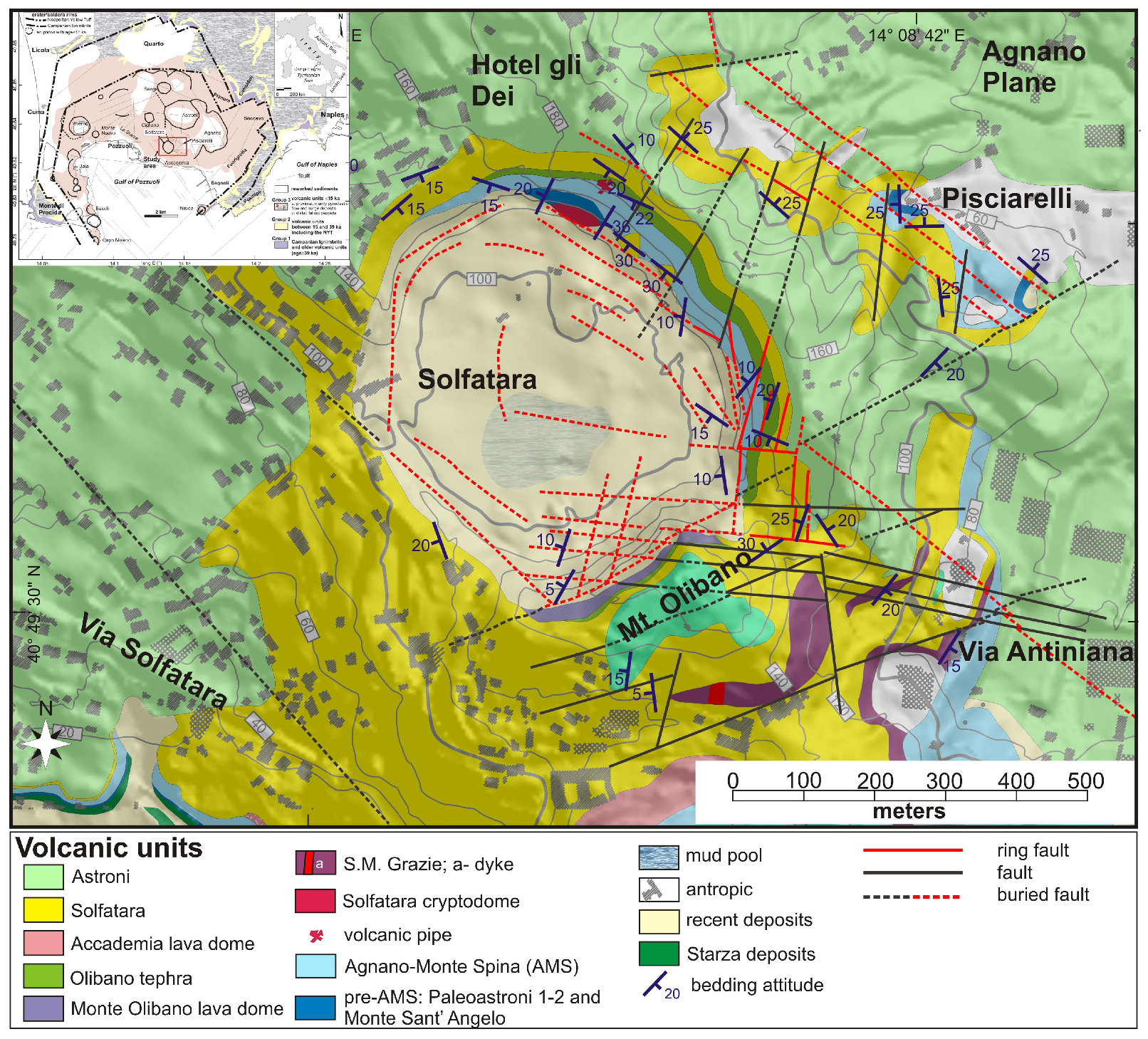
2. Study Area
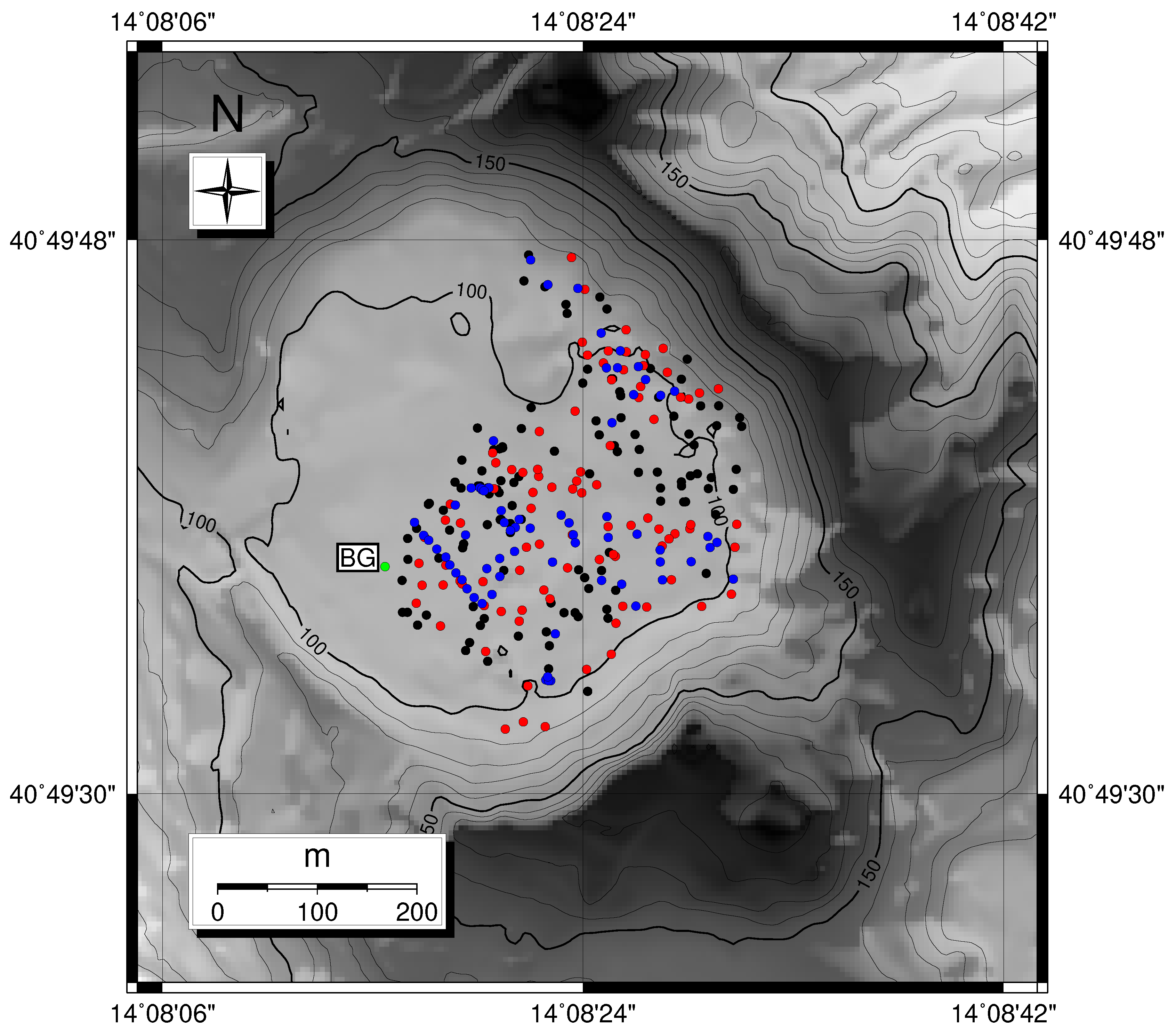
3. Materials and Methods
3.1. Materials
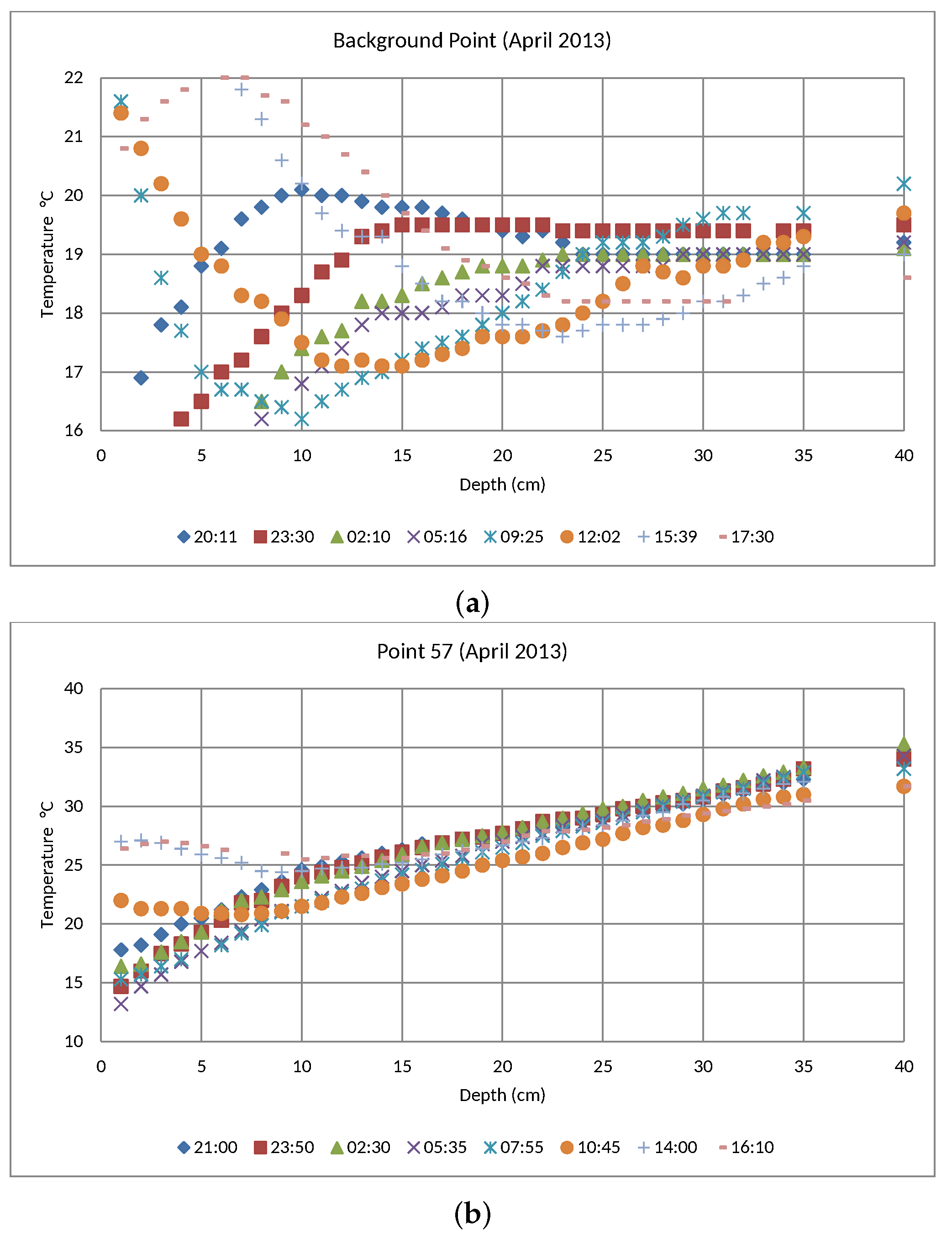
3.1.1. Measurement of the Soil Temperature by IR Camera
3.1.2. Measurement of the Temperature Gradient of the Soil
3.2. Methods
3.2.1. Summary of the Procedure
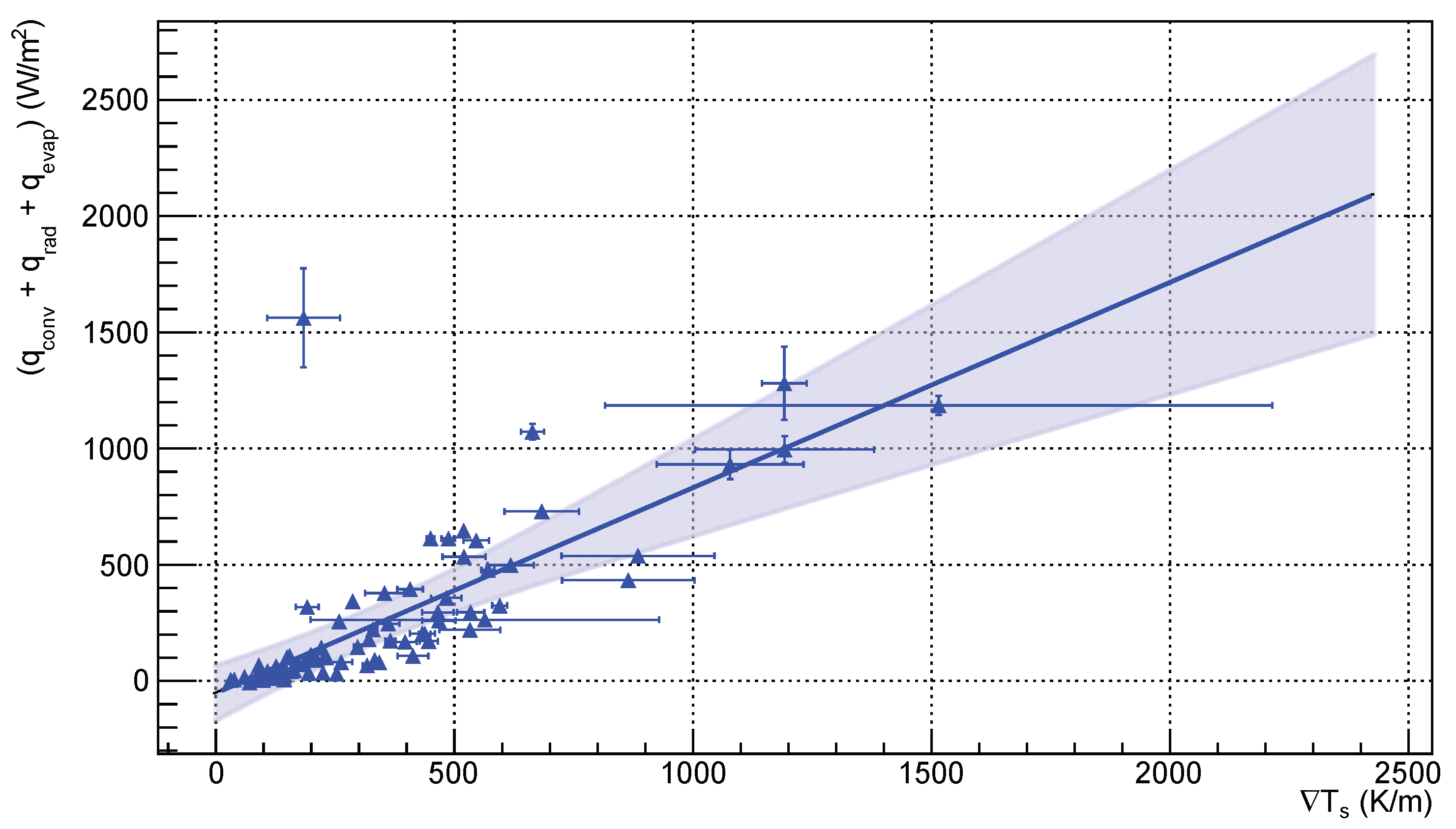
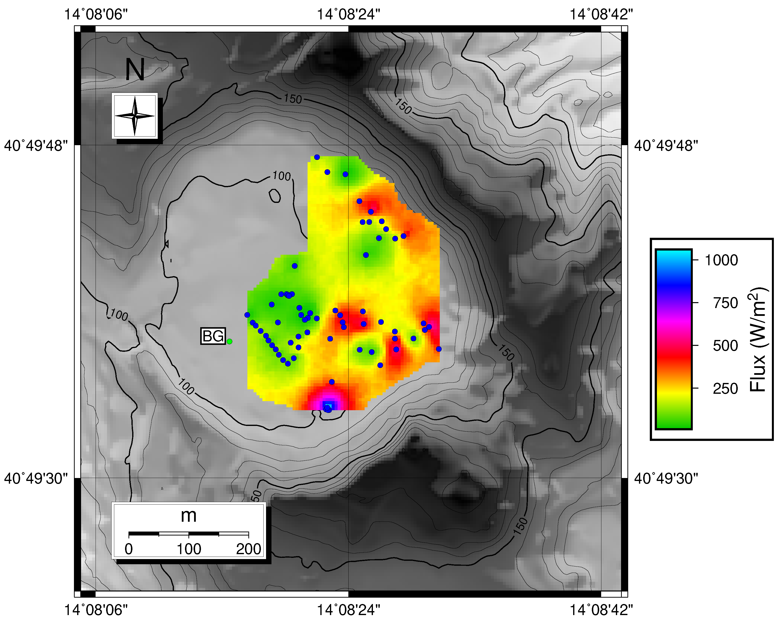
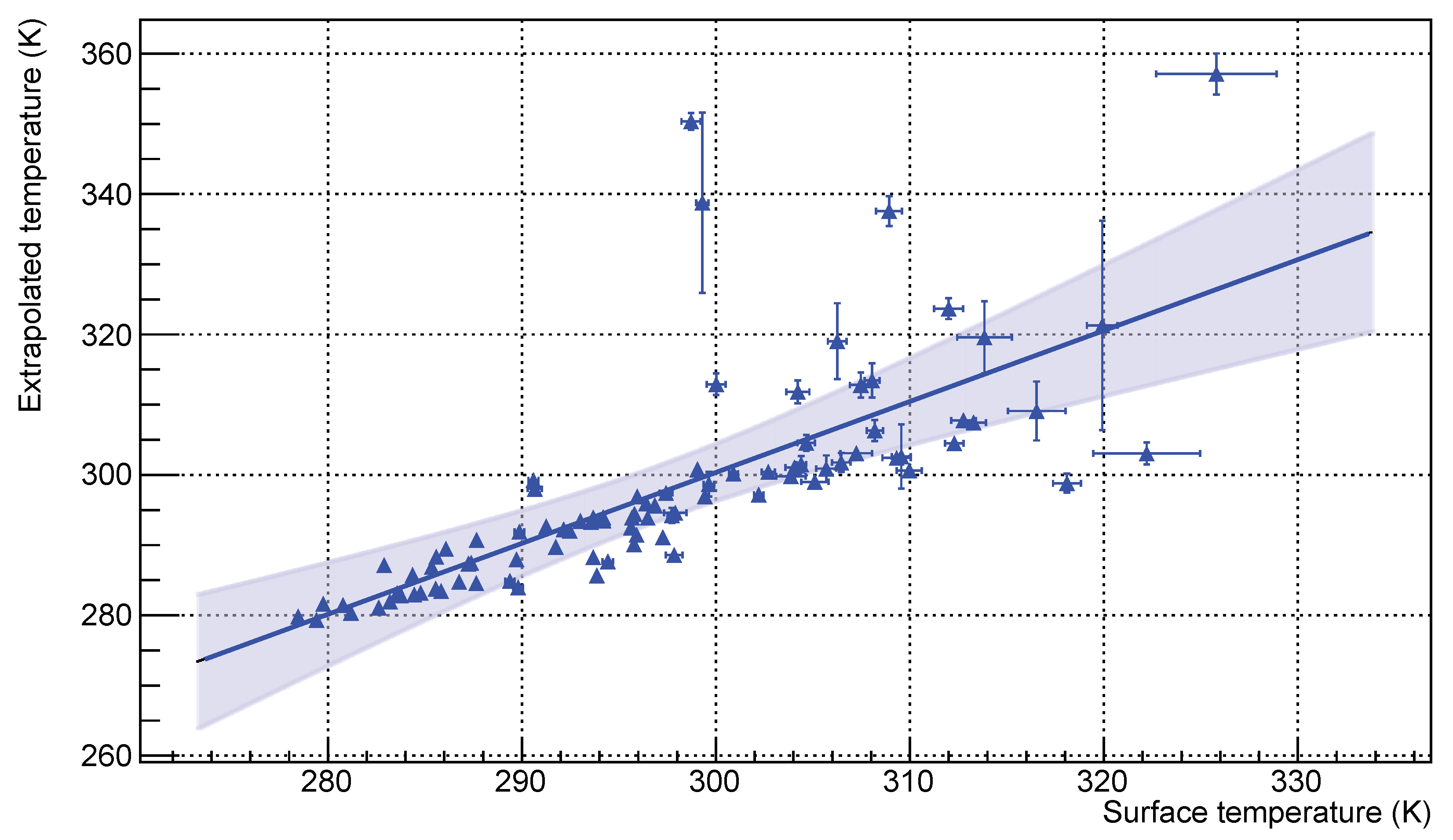
4. Results
5. Discussion
6. Conclusions
Supplementary Materials
Author Contributions
Funding
Acknowledgments
Conflicts of Interest
Abbreviations
| CL | Confidence Level |
| DDS | Diffuse Degassing Structure |
| CFc | Campi Flegrei caldera |
| IR | Infra Red |
| sGs | sequential Gaussian simulations |
| RPAS | Remotely Piloted Aircraft System |
References
- Noguchi, K.; Kamiya, H. Prediction of volcanic eruption by measuring the chemical composition and amounts of gases. Bull. Volcanol. 1963, 26, 367–378. [Google Scholar] [CrossRef]
- Baxter, P.J.; Baubron, J.C.; Coutinho, R. Health hazards and disaster potential of ground gas emissions at Furnas volcano, São Miguel, Azores. J. Volcanol. Geotherm. Res. 1999, 92, 95–106. [Google Scholar] [CrossRef]
- Chiodini, G.; Frondini, F.; Cardellini, C.; Granieri, D.; Marini, L.; Ventura, G. CO2 degassing and energy release at Solfatara volcano, Campi Flegrei, Italy. J. Geophys. Res. 2001, 106, 16213–16221. [Google Scholar] [CrossRef]
- Chiodini, G.; Granieri, D.; Avino, R.; Caliro, S.; Costa, A.; Werner, C. Carbon dioxide diffuse degassing: Implications on the energetic state of a volcanic hydrothermal systems. J. Geophys. Res. 2005, 110, B08204. [Google Scholar] [CrossRef]
- Frondini, F.; Chiodini, G.; Caliro, S.; Cardellini, C.; Granieri, D.; Ventura, G. Diffuse CO2 degassing at Vesuvio, Italy. Bull. Volcanol. 2004, 66, 642–651. [Google Scholar] [CrossRef]
- Chiodini, G.; Vilardo, G.; Augusti, V.; Granieri, D.; Caliro, S.; Minopoli, C.; Terranova, C. Thermal monitoring of hydrothermal activity by permanent infrared automatic stations: Results obtained at Solfatara di Pozzuoli, Campi Flegrei (Italy). J. Geophys. Res. 2007, 112, B12206. [Google Scholar] [CrossRef]
- Granieri, D.; Carapezza, M.L.; Chiodini, G.; Avino, R.; Caliro, S.; Ranaldi, M.; Ricci, T.; Tarchini, L. Correlated increase in CO2 fumarolic content and diffuse emission from La Fossa crater (Vulcano, Italy): Evidence of volcanic unrest or increasing gas release from a stationary deep magma body? Geophys. Res. Lett. 2006, 33, L13316. [Google Scholar] [CrossRef]
- Chiodini, G.; Vandemeulebrouck, J.; Caliro, S.; D’Auria, L.; De Martino, P.; Mangiacapra, A.; Petrillo, Z. Evidence of thermal-driven processes triggering the 2005-2014 unrest at Campi Flegrei caldera. Earth Planet. Sci. Lett. 2015, 414, 58–67. [Google Scholar] [CrossRef]
- Caliro, S.; Chiodini, G.; Paonita, A. Geochemical evidences of magma dynamics at Campi Flegrei (Italy). Geochim. Cosmochim. Acta 2014, 132, 1–15. [Google Scholar] [CrossRef]
- Hochstein, M.P.; Bromley, C.J. Measurement of heat flux from steaming ground. Geothermics 2005, 34, 133–160. [Google Scholar] [CrossRef]
- Friedman, J.D.; Williams, D.L.; Frank, D. Structural and heat flow implications of infrared anomalies at Mt. Hood, Oregon, 1972–1977. J. Geophys. Res. Solid Earth 1982, 87, 2793–2803. [Google Scholar] [CrossRef]
- Frank, D. Hydrothermal Processes at Mount Rainier, Washington. Ph.D. Thesis, Washington University, Seattle, WA, USA, 1985. [Google Scholar]
- Aubert, M. Pratical evaluation of steady heat discharge from dormant active volcanoes: Case study of Vulcarolo fissure (Mount Etna, Italy). J. Volcanol. Geotherm. Res. 1999, 92, 413–429. [Google Scholar] [CrossRef]
- Aubert, M.; Diliberto, S.; Finizola, A.; Chébli, Y. Double origin of hydrothermal convective flux variations in the Fossa of Vulcano (Italy). Bull. Volcanol. 2008, 70, 743–751. [Google Scholar] [CrossRef]
- Oppenheimer, C. Infrared surveillance of crater lakes using satellite data. J. Volcanol. Geotherm. Res. 1993, 55, 117–128. [Google Scholar] [CrossRef]
- Wright, R.; Blake, S.; Harris, A.; Rothery, D. A simple explanation for the space-based calculation of lava eruptions rates. Earth Planet. Sci. Lett. 2001, 192, 223–233. [Google Scholar] [CrossRef]
- Sekioka, M.; Yuhara, K. Heat flux estimation in geothermal areas based on the heat balance of the ground surface. J. Geophys. Res. 1974, 79, 2053–2058. [Google Scholar] [CrossRef]
- Yuhara, K.; Sekioka, M.; Ehara, S. Infrared measurement on Satsuma-iwojima Island, Kagoshima, Japan, by helicopter-borne thermocamera. Arch. Met. Geoph. Biokl. A 1978, 27, 171–181. [Google Scholar] [CrossRef]
- Yuhara, K.; Ehara, S.; Tagomori, K. Estimation of heat discharge rates using infrared measurements by a helicopter-borne thermocamera over the geothermal areas of Unzen volcano, Japan. J. Volcanol. Geotherm. Res. 1981, 9, 99–109. [Google Scholar] [CrossRef]
- Stevenson, J.A.; Varley, N. Fumarole monitoring with a handheld infrared camera: Volcán de Colima, Mexico, 2006–2007. J. Volcanol. Geotherm. Res. 2008, 177, 911–924. [Google Scholar] [CrossRef]
- Vilardo, G.; Sansivero, F.; Chiodini, G. Long-term TIR imagery processing for spatiotemporal monitoring of surface thermal features in volcanic environment: A case study in the Campi Flegrei (Southern Italy). J. Geophys. Res. Solid Earth 2015, 120, 812–826. [Google Scholar] [CrossRef] [Green Version]
- Gaudin, D.; Beauducel, F.; Allemand, P.; Delacourt, C.; Finizola, A. Heat flux measurement from thermal infrared imagery in low-flux fumarolic zones: Example of the Ty fault (La Soufriŕe de Guadeloupe). J. Volcanol. Geotherm. Res. 2013, 267, 47–56. [Google Scholar] [CrossRef]
- Stevenson, D.S. Physical models of fumarolic flow. J. Volcanol. Geotherm. Res. 1993, 57, 139–156. [Google Scholar] [CrossRef]
- Wooster, M.J.; Rothery, D.A. Thermal monitoring of Lascar volcano, Chile, using infrared data from the along track scanning radiometer: A 1992–1995 time series. Bull. Volcanol. 1997, 58, 566–579. [Google Scholar] [CrossRef]
- Harris, A.J.L.; Stevenson, D.S. Thermal observations of degassing open conduits and fumaroles at Stromboli and Vulcano using remotely sensed data. J. Volcanol. Geotherm. Res. 1997, 76, 175–198. [Google Scholar] [CrossRef]
- Kaneko, T.; Wooster, M.J. Landsat infrared analysis of fumarole activity at Unzen volcano: Time series comparison with gas and magma fluxes. J. Volcanol. Geotherm. Res. 1999, 89, 57–64. [Google Scholar] [CrossRef]
- Pieri, D.; Abrams, M. ASTER observations of thermal anomalies preceding the April 2003 eruption of Chikurachki volcano, Kurile Islands, Russia. Remote Sens. Environ. 2005, 99, 84–94. [Google Scholar] [CrossRef]
- Spampinato, L.; Calvari, S.; Oppenheimer, C.; Boschi, E. Volcano surveillance using infrared cameras. Earth Sci. Rev. 2011, 106, 63–91. [Google Scholar] [CrossRef]
- Isaia, R.; Vitale, S.; Di Giuseppe, M.G.; Iannuzzi, E.; D’Assisi Tramparulo, F.; Troiano, A. Stratigraphy, structure, and volcano-tectonic evolution of Solfatara maar-diatreme (Campi Flegrei, Italy). Geol. Soc. Am. Bull. 2015, 127, 1485–1504. [Google Scholar] [CrossRef]
- Cardellini, C.; Chiodini, G.; Frondini, F.; Avino, R.; Bagnato, E.; Caliro, S.; Lelli, M.; Rosiello, A. Monitoring diffuse volcanic degassing during volcanic unrests: The case of Campi Flegrei (Italy). Sci. Rep. 2017, 7, 6757. [Google Scholar] [CrossRef]
- Granieri, D.; Avino, R.; Chiodini, G. Carbon dioxide diffuse emission from the soil: Ten years of observations at Vesuvio and Campi Flegrei (Pozzuoli), and linkages with volcanic activity. Bull. Volcanol. 2010, 72, 103–118. [Google Scholar] [CrossRef]
- Di Vito, M.A.; Isaia, R.; Orsi, G.; Southon, J.; de Vita, S.; D’Antonio, M.; Pappalardo, L.; Piochi, M. Volcanism and deformation since 12,000 years at the Campi Flegrei caldera (Italy). J. Volcanol. Geotherm. Res. 1999, 91, 221–246. [Google Scholar] [CrossRef]
- Orsi, G.; Civetta, L.; Del Gaudio, C.; de Vita, S.; Di Vito, M.A.; Isaia, R.; Petrazzuoli, S.M.; Ricciardi, G.P.; Ricco, C. Short-term ground deformations and seismicity in the resurgent Campi Flegrei caldera Italy: An example of active block-resurgence in a densely populated area. J. Volcanol. Geotherm. Res. 1999, 91, 415–451. [Google Scholar] [CrossRef]
- Petrosino, S.; Damiano, N.; Cusano, P.; Di Vito, M.A.; de Vita, S.; Del Pezzo, E. Subsurface structure of the Solfatara volcano (Campi Flegrei caldera, Italy) as deduced from joint seismic-noise array, volcanological and morphostructural analysis. Geochem. Geophys. Geosyst. 2012, 13, 1–25. [Google Scholar] [CrossRef]
- Bruno, P.P.G.; Ricciardi, G.P.; Petrillo, Z.; Di Fiore, V.; Troiano, A.; Chiodini, G. Geophysical and hydrogeological experiments from a shallow hydrothermal system at Solfatara Volcano, Campi Flegrei, Italy: Response to caldera unrest. J. Geophys. Res. 2007, 112, B06201. [Google Scholar] [CrossRef]
- Byrdina, S.; Vandemeulebrouck, J.; Cardellini, C.; Legaz, A.; Camerlynck, C.; Chiodini, G.; Lebourg, T.; Gresse, M.; Bascou, P.; Motos, G.; et al. Relations between electrical resistivity, carbon dioxide flux, and self-potential in the shallow hydrothermal system of Solfatara (Phlegrean Fields, Italy). J. Volcanol. Geotherm. Res. 2014, 283, 172–182. [Google Scholar] [CrossRef]
- Gresse, M.; Vandemeulebrouck, J.; Byrdina, S.; Chiodini, G.; Revil, A.; Johnson, T.C.; Ricci, T.; Vilardo, G.; Mangiacapra, A.; Lebourg, T.; et al. Three-dimensional electrical resistivity tomography of the Solfatara crater (Italy): Implication for the multiphase flow structure of the shallow hydrothermal system. J. Geophys. Res. Solid Earth 2017, 122, 8749–8768. [Google Scholar] [CrossRef]
- De Siena, L.; Del Pezzo, E.; Bianco, F. Seismic attenuation imaging of Campi Flegrei: Evidence of gas reservoirs, hydrothermal basins, and feeding systems. J. Geophys. Res. 2010, 115, B09312. [Google Scholar] [CrossRef]
- Battaglia, J.; Zollo, A.; Virieux, J.; Dello Iacono, D. Merging active and passive data sets in traveltime tomography: The case study of Campi Flegrei caldera (Southern Italy). Geophys. Prospect. 2008, 56, 555–573. [Google Scholar] [CrossRef]
- Marotta, E.; Calvari, S.; Cristaldi, A.; D’Auria, L.; Di Vito, M.A.; Moretti, R.; Peluso, R.; Spampinato, L.; Boschi, E. Reactivation of Stromboli’s summit craters at the end of the 2007 effusive eruption detected by thermal surveys and seismicity. J. Geophys. Res. 2015, 120, 7376–7395. [Google Scholar] [CrossRef]
- Connor, C.B.; Clement, B.M.; XiaoDan, S.; Lane, S.B.; West-Thomas, J. Continuous monitoring of high-temperature fumaroles on an active lava dome, Volcán Colima, Mexico: Evidence of mass flow variation in response to atmospheric forcing. J. Geophys. Res. 1993, 98, 19713–19722. [Google Scholar] [CrossRef]
- Finizola, A.; Ricci, T.; Deiana, R.; Barde Cabusson, S.; Rossi, M.; Praticelli, N.; Giocoli, A.; Romano, G.; Delcher, E.; Suski, B.; et al. Adventive hydrothermal circulation on Stromboli volcano (Aeolian Islands, Italy) revealed by geophysical and geochemical approaches: Implications for general fluid flow models on volcanoes. J. Volcanol. Geotherm. Res. 2010, 196, 111–119. [Google Scholar] [CrossRef]
- Richter, G.; Wassermann, J.; Zimmer, M.; Ohrnberger, M. Correlation of seismic activity and fumarole temperature at the Mt. Merapi volcano (Indonesia) in 2000. J. Volcanol. Geotherm. Res. 2004, 135, 331–342. [Google Scholar] [CrossRef]
- Finizola, A.; Revil, A.; Rizzo, E.; Piscitelli, S.; Ricci, T.; Morin, J.; Angeletti, B.; Mocochain, L.; Sortino, F. Hydrogeological insights at Stromboli volcano (Italy) from geoelectrical, temperature, and CO2 soil degassing investigations. Geophys. Res. Lett. 2006, 33, L17304. [Google Scholar] [CrossRef]
- Flynn, L.P.; Mouginis-Mark, P.J.; Gradie, J.C.; Lucey, P.G. Radiative temperature measurements at Kupaianaha Lava Lake, Kilauea Volcano, Hawaii. J. Geophys. Res. Solid Earth 1993, 98, 6461–6476. [Google Scholar] [CrossRef]
- Pinkerton, H.; James, M.; Jones, A. Surface temperature measurements of active lava flows on Kilauea volcano, Hawai’i. J. Volcanol. Geotherm. Res. 2002, 113, 159–176. [Google Scholar] [CrossRef]
- Peltier, A.; Finizola, A. Douillet, G.A.; Brothelande, E.; Garaebiti, E. Structure of an active volcano associated with a resurgent block inferred from thermal mapping: The Yasur-Yenkahe volcanic complex (Vanuatu). J. Volcanol. Geotherm. Res. 2012, 243-244, 59–68. [Google Scholar] [CrossRef]
- Al-Arabi, M.; El-Riedy, M.K. Natural convection heat transfer from horizontal plates of different shapes. Int. J. Heat Mass Trans. 1976, 19, 1399–1404. [Google Scholar] [CrossRef]
- Incropera, F.P.; DeWitt, D.P. Fundamentals of Heat and Mass Transfer, 4th ed.; John Wiley & Sons Ltd.: Hoboken, NJ, USA, 1996. [Google Scholar]
- Jacobson, M.Z. Fundamentals of Atmospheric Modelling, 2nd ed.; Cambridge University Press: New York, NY, USA, 2005. [Google Scholar]
- Cardellini, C.; Chiodini, G.; Frondini, F. Application of stochastic simulation to CO2 flux from soil: Mapping and quantification of gas release. J. Geophys. Res. 2003, 108, 2425–2438. [Google Scholar] [CrossRef]
- Deutsch, C.V.; Journel, A.G. GSLIB Geostatistical Software Library and User’s Guide, 2nd ed.; Oxford Univerity Press: Oxford, UK, 1998; Volume 136. [Google Scholar]
- Sawyer, G.M.; Burton, M.R. Effects of a volcanic plume on thermal imaging data. Geophys. Res. Lett. 2006, 33. [Google Scholar] [CrossRef] [Green Version]
- Ball, M.; Pinkerton, H. Factors affecting the accuracy of thermal imageing cameras in volcanology. J. Geophys. Res. 2006, 111. [Google Scholar] [CrossRef]
- Todesco, M.; Chiodini, G.; Macedonio, G. Monitoring and modeling hydrothermal fluid emission at La Solfatara (Phlegrean Fields, Italy). An interdisciplinary approach to the study of diffuse degassing. J. Volcanol. Geotherm. Res. 2003, 125, 57–79. [Google Scholar] [CrossRef]


| Model | FLIR SC640 |
|---|---|
| Detector Type | Uncooled Microbolometer, FPA (Focal Plane Array) |
| Resolution | pixel |
| Spectral range | m |
| Precision | ±C or of reading |
| Thermal sensitivity | <C at C |
| Focal length | 37.64 mm |
| Spatial resolution | 0.66 mrad |
| Description | Symbol | Value | Unit |
|---|---|---|---|
| Typical parameters (evaluated at ) | |||
| Atmospheric pressure (assumed constant) | Pa | ||
| Diffusion coefficient of vapor in air | m/s | ||
| Lewis number | 0.857 | — | |
| Kinematic viscosity of the air | m/s | ||
| Molecular weight of air | kg/mol | ||
| Molecular weight of water | kg/mol | ||
| Relative emissivity of the surface | 0.98 | — | |
| Specific heat of air at constant pressure | 1004.67 | J/kg K | |
| Stefan-Boltzmann constant | W/m K | ||
| Thermal conductivity of the air | W/mK | ||
| Thermal expansion coefficient of the air | 1/K | ||
| Thermal diffusivity of the air | m/s | ||
| Results from best fits and estimates. | |||
| Thermal conductivity of the soil | W/(K · m) | ||
| Total power released through the investigated surface | MW | ||
| Average heat flux on the investigated surface | |||
© 2019 by the authors. Licensee MDPI, Basel, Switzerland. This article is an open access article distributed under the terms and conditions of the Creative Commons Attribution (CC BY) license (http://creativecommons.org/licenses/by/4.0/).
Share and Cite
Marotta, E.; Peluso, R.; Avino, R.; Belviso, P.; Caliro, S.; Carandente, A.; Chiodini, G.; Macedonio, G.; Avvisati, G.; Marfè, B. Thermal Energy Release Measurement with Thermal Camera: The Case of La Solfatara Volcano (Italy). Remote Sens. 2019, 11, 167. https://doi.org/10.3390/rs11020167
Marotta E, Peluso R, Avino R, Belviso P, Caliro S, Carandente A, Chiodini G, Macedonio G, Avvisati G, Marfè B. Thermal Energy Release Measurement with Thermal Camera: The Case of La Solfatara Volcano (Italy). Remote Sensing. 2019; 11(2):167. https://doi.org/10.3390/rs11020167
Chicago/Turabian StyleMarotta, Enrica, Rosario Peluso, Rosario Avino, Pasquale Belviso, Stefano Caliro, Antonio Carandente, Giovanni Chiodini, Giovanni Macedonio, Gala Avvisati, and Barbara Marfè. 2019. "Thermal Energy Release Measurement with Thermal Camera: The Case of La Solfatara Volcano (Italy)" Remote Sensing 11, no. 2: 167. https://doi.org/10.3390/rs11020167