Article

Flash Flood Risk Analysis Based on Machine Learning Techniques in the Yunnan Province, China

1
China Institute of Water Resources and Hydropower Research, Beijing 100038, China
2
College of water sciences, Beijing Normal University, Beijing 100875, China
3
School of Geographical Sciences, University of Bristol, Bristol BS8 1SS, UK
4
Department of Geological Sciences University of Texas at San Antonio, San Antonio, TX 78249, USA
5
CITIC Construction Co., Ltd., Beijing 100027, China
6
Lab of Spatial Information Integration, Institute of Remote Sensing and Digital Earth, Chinese Academy of Sciences, Beijing 100101, China
7
School of Earth and Space Sciences, Peking University, Beijing 100871, China
*
Authors to whom correspondence should be addressed.
Remote Sens. 2019, 11(2), 170; https://doi.org/10.3390/rs11020170
Submission received: 6 November 2018 / Revised: 7 January 2019 / Accepted: 11 January 2019 / Published: 17 January 2019
(This article belongs to the Special Issue Advances in Remote Sensing-based Disaster Monitoring and Assessment)

Abstract

:
Flash flood, one of the most devastating weather-related hazards in the world, has become more and more frequent in past decades. For the purpose of flood mitigation, it is necessary to understand the distribution of flash flood risk. In this study, artificial intelligence (Least squares support vector machine: LSSVM) and classical canonical method (Logistic regression: LR) are used to assess the flash flood risk in the Yunnan Province based on historical flash flood records and 13 meteorological, topographical, hydrological and anthropological factors. Results indicate that: (1) the LSSVM with Radial basis function (RBF) Kernel works the best (Accuracy = 0.79) and the LR is the worst (Accuracy = 0.75) in testing; (2) flash flood risk distribution identified by the LSSVM in Yunnan province is near normal distribution; (3) the high-risk areas are mainly concentrated in the central and southeastern regions, where with a large curve number; and (4) the impact factors contributing the flash flood risk map from higher to low are: Curve number > Digital elevation > Slope > River density > Flash Flood preventions > Topographic Wetness Index > annual maximum 24 h precipitation > annual maximum 3 h precipitation.

1. Introduction

Flash flood is one of the most devastating natural disasters with characteristics of high-velocity runoff, short lead-time and fast-rising water [1]. Economic losses caused by flash flood increase year by year with the increase of population and infrastructure in flood-prone areas [2]. For instance, a total of 28,826 flash flood events happened in the United States between 2007 and 2015 and 10% of flash flood resulted in damages exceeding $100,000 [3]. According to the China Floods and Droughts Disasters Bulletin of 2015, an average of 935 people dies each year by flash flood disasters from 2000 to 2015. Owing to the impact of climate change, the flash flood risk is predicted to increase with the frequent extreme precipitation and sea level rise [4]. Therefore, an accurate risk assessment is critical for flash flood prevention.
Flash floods risk is a combination of flood hazard and vulnerability of an area [5,6]. Flood risk is widely assessed by hydrological models or data-driven model based on historical flood inventories. The hydrological model has a clear physical mechanism that reflects the process of flood generation and transportation. One of the most widely used models is 1–2-dimension routing model such as MIKE 21, which can truly reflect the flooding scope and water depth during flooding. The flood risk is assessed by combining water depth and local vulnerability [7,8]. However, since the simulation of the actual hydrological process is affected by many factors (e.g., model’s parameter, structure, input data), the model accuracy and uncertainty need to be further explored [9]. Meanwhile, different regions require different types of hydrological models, resulting in high data requirements and time-consuming on model development [10,11].
In terms of this, data-driven models were proposed for flood risk assessment. Data-driven models adopt black-box models and uses various intelligent algorithms to establish optimal mathematical relationships between disaster and explanatory factors, such as analytic hierarchy process (AHP), set pair analysis method (SPAM) and so forth. AHP is a simple and effective multi-criteria decision-making method, which effectively solves the lack of quantitative data in flood risk assessment and the complex relationship involving multiple risk factors [12]. SPAM is a method for systematic analysis of uncertain problems, effectively dealing with the incompleteness of information for flood risk prediction [13]. However, AHP and SPAM are all based on expert opinions in choosing the indicator weighting that introducing uncertainty and subjectivity in assessment [14]. With the development of artificial intelligence, machine learning (ML) models, including support vector machine (SVM), Random Forest (RF) and Decision Tree (DT), has been proposed and applied in flood risk assessment. Machine learning models avoid the subjective determination of weights by learning the relationship between flood risk and explanatory factors. Among them, SVM is a popular ML model that can solve linear and nonlinear regression problems and has gained extensive applications in pattern recognition, data mining and speech recognition [15]. Least Squares Support Vector Machine (LSSVM) is a simple SVM that uses least squares and linear equations to improve model efficiency [16]. Flash flood data is often complex and incomplete and the relationships between variables can be strongly nonlinear and involve high-order interactions. Therefore, it is of great value to explore the flash flood risk assessment by LSSVM method.
Nowadays, with the in-depth application of 3S technologies (Remote Sensing, Geography Information Systems and Global Positioning Systems) in hydrology, the acquisition of spatial information on the underlying surface of the basin have been significantly improved [17]. Meanwhile, a series of intelligent algorithms based on big data have been proposed that are valuable to use in hydrology. In this study, we developed a flash flood assessment framework based on machine learning models. We utilize the LSSVM method with three kernel functions (linear: LN; radial basis function: RBF; polynomial: PL) and classical logistic regression (LR) method to assess flash flood risk based on the official statistics of flash flood events. The performances of our proposed method are evaluated with five indices and ROC curve in Section 3.1. The distribution of flash flood risk in the study area and the relationship between flood risk and flood trigger factors are discussed in Section 3.2.

2. Materials and Methods

2.1. Study Area

Yunnan Province (20°8’–29°16’N, 97°31’–106°12’E) is located in southwestern China with an area of 383,210 km2. It is one of the most flooded provinces in China and the economy relies mainly on natural resources. In 2016, Yunnan province had a population of 47.7 million, a gross domestic product (GDP) of 1.49 billion yuan. Yunnan province is located in the low latitude plateau and the terrain is dominated by mountains, with a canyon in the west, a plateau in the east and a major river running through the deep valley. From the southeastern mountainous area to the northwest Hengduan Mountains, the altitude ranges from less than 100 m to more than 6000 m, with an average elevation of 1980 m. The mountainous area, plateau area and watershed area account for 80%, 12.5% and 7.5% of the total area respectively. About 39% of slopes exceed 25° in mountainous areas and the slopes of the northeast and northwest mountainous areas even reach 60–90%. The soil texture is loose, of which more than 50% is krasnozem. The climate is mainly affected by atmospheric circulation, which is a low mountain monsoon climate. The annual average precipitation is 1102 mm, with significant spatial-temporal differences [18]. Meanwhile, extreme weather events occur frequently, especially during the summer flood season (June to September), with rainfall accounting for 85–95% between May and October.
China has implemented the construction of non-structural measures for flash flood prevention since 2011. In Yunnan Province, there are 206 flash floods events from 2011 to 2015, causing 237 deaths. Especially in 2014 and 2015, the number of deaths accounted for 22.2% and 8.1% of the national total, respectively, which were the most affected by the flash floods. In order to defend against flash flood, Yunnan has launched the construction of non-structural flood prevention measures covering 129 counties since 2010. The average construction fund is $0.87 million for each county. The preventive measures implemented include: encrypting automatic rainfall stations to improve the quality of monitoring data, installing simple rainfall equipment with alarms, building an alarm system consisting of radio broadcasts and simple alarm devices. Obviously, although Yunnan Province already has a certain defense base, it still suffers from severe flash flood disasters. Therefore, it is of great significance to study the flash flood risk in Yunnan Province. Figure 1 shows the historical flash floods in Yunnan Province from 2011 to 2015. Obviously, flash floods mainly occur on lower slopes, mainly because the air rises on the windward slope and the water vapor condenses easily to form precipitation, which causes runoff to accumulate in the valley and triggers flash floods. The leeward slope is not easy to form precipitation due to the air sinking and the temperature moving downward [19].

2.2. Data

The flash flood records are mainly from official authoritative departments, such as the Ministry of Water Resources (MWR), the Ministry of Land and Resources and some local government agencies in Yunnan province. These data are divided into training and testing datasets, 70% of which are randomly selected for training and the remaining 30% data for testing. The principle of the distribution ratio is that the samples are evenly distributed and have certain representativeness (Figure 1). It is important to emphasize that all the flash floods studied in this paper involve death or missing; regardless of incidents that do not cause casualties. The remote sensing data and other data covered in this paper are shown in Table 1.

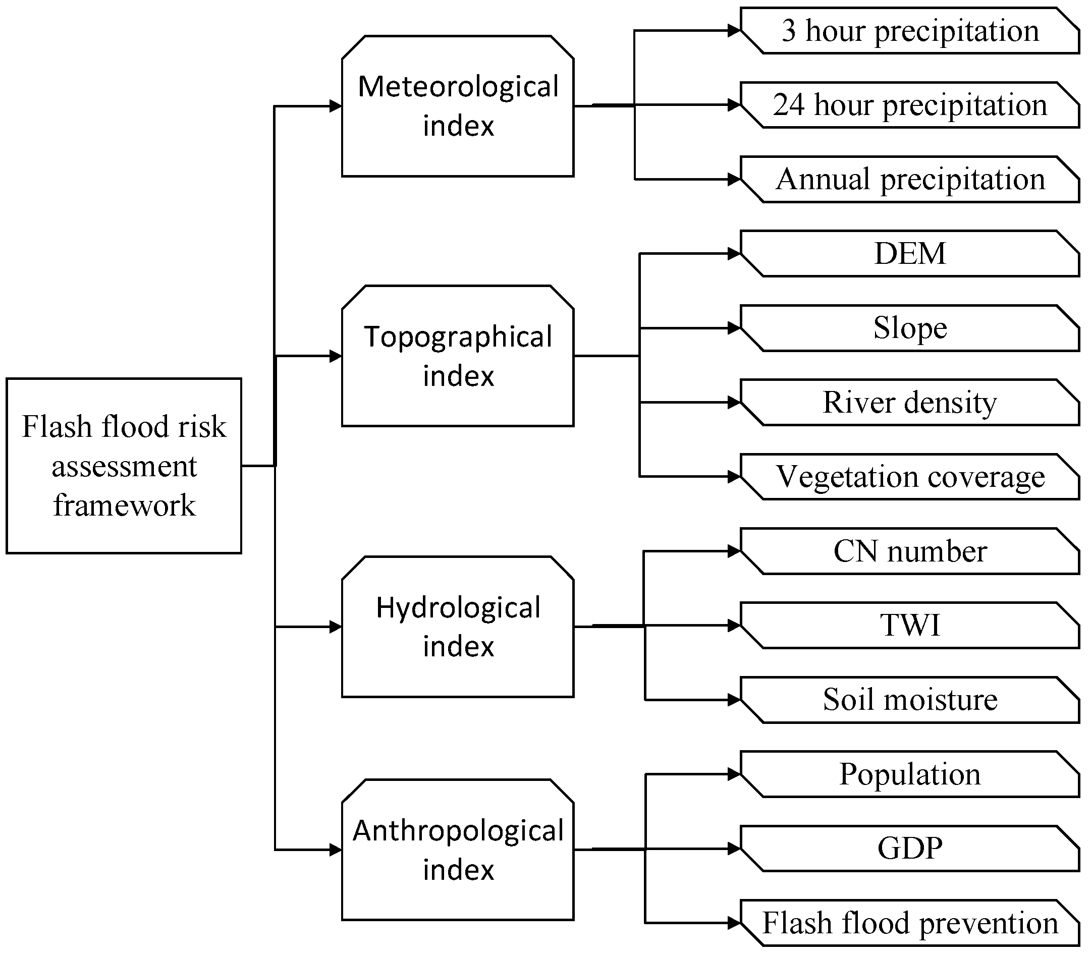
2.3. Flash Flood Triggering Factors

Flash flood disasters are mainly affected by meteorological, topographical hydrological, anthropological factors. The related factors affecting flash flood risk are shown in Figure 2 and are described as followed:
(1) Meteorological factors
Three meteorological factors including 3-H-P, 24-H-P and AP are the main factors leading to flash floods, with 3-H-P and 24-H-P reflecting the frequency and characteristics of short-term rainfall and AP reflecting the characteristics of long-term rainfall. The precipitation data comes from the China Meteorological Forcing Dataset (CMFD), produced by the Institute of Tibetan Plateau Research, Chinese Academy of Sciences (hereafter ITPCAS). The dataset is based primarily on the existing Princeton reanalysis data, Global Land Data Assimilation System (GLDAS) data, Global Energy and Water cycle Experiment—Surface Radiation Budget (GEWEX-SRB) radiation data and Tropical Rainfall Measuring Mission (TRMM) precipitation data in the world, combined conventional CMA weather observations were produced with temporal and spatial resolutions of 3 h and 0.1° × 0.1°, respectively.
(2) Topographical factors
Digital elevation model (DEM) retrieved from NASA SRTM, a 90-m raster in 2000. DEM resolution mainly affects the watershed topography, which in turn affects the accuracy of runoff generation and convergence. The higher the DEM resolution, the higher the accuracy of the extracted watershed features. However, high-resolution DEM over-emphasizes the computational burden of the model, greatly restricting the runtime of the model [20]. Slope (SL) refers to the ratio of the vertical height of the slope to the horizontal direction, which is suitable for the sensitivity analysis of floods. Generally, the SL is calculated from the DEM data using the ArcGIS tool [17]. River density (RD) utilizes China’s basic vector format dataset, which is related to the area of the grid and the length of the river in the grid [21]. Vegetation coverage (VC) is calculated by an average multi-year normalized difference vegetation index (NDVI) based on MODIS images. It represents vegetation distribution and biomass levels from 2011 to 2015 [22].
(3) Hydrological factors
The Curve Number (CN) derived from the soil conservation service curve number (SCS-CN) model is a comprehensive indicator calculated according to the National Engineering Handbook of US, which primarily reflects the potential capacity of runoff generation in different grids. It is a non-dimensional index with a theoretical value between 0 (no runoff) and 100 (no infiltration). For details of CN, please refer to Zeng et al. (2017) [23]. The topographic wetness index (TWI), combined with the local uphill contribution area and the entire slope, is widely used to quantify the topographical control of flood concentration processes and can be calculated from DEM [24]. Soil moisture (SM) data is from the European Space Agency (ESA) with a spatial accuracy of 50 km. It can estimate moisture in the soil surface (down to 5 cm) which is important for hydrological modeling. SM indicates the non-linear partitioning of the precipitation into infiltration and runoff, affecting runoff by affecting infiltration [25].
(4) Anthropological factors
The effects of flood risks are often related to anthropology, manifested as loss of economic property and casualties. The losses generally increase with the population growth in flood-prone areas, especially in economically developed and densely populated areas. Therefore, Gross Domestic Product (GDP) and population (Pop) are selected as anthropological factors for flash flood assessment. DDP is defined as “an aggregate measure of production equal to the sum of the gross values added of all resident and institutional units engaged in production (plus any taxes and minus any subsidies, on products not included in the value of their outputs), mainly reflecting the economic situation of the study area. Moreover, GDP is a total indicator, which basically organizes indicators describing various aspects of the national economy through a series of scientific principles and methods. Therefore, GDP contained contributing indicators such as over-exploitation [26]. The 1-km gridded GDP and population of Yunnan Province are collected from the Data Center for Resources and Environmental Sciences Chinese Academy of Sciences (RESDC). In 2010, the Chinese government initiated the construction of national-level non-structural measures for flash flood prevention. This investment is the largest non-structural project in China, involving a total area of 3.86 million km2 in 29 provinces (autonomous regions and municipalities). The preventive measures include the national flash flood investigation and evaluation, the establishment of construction monitoring and early warning platforms, automatic rainfall stations and water level stations, mass observations and mass prevention and so forth. The FFP data is mainly from the MWR and local governments and utilizing the investment funds to comprehensively reflect the flash flood prevention situation [27,28]. The related factors affecting flash flood risk in the LSSVM method are shown in Figure 3.

2.4. Methodology

(1) LSSVM
LSSVM utilizes a set of linear equations to minimize the complexity of the optimization process. The constraint optimization problems can be solved using Lagrange multipliers. Consider a given training set x i ,   y i ,   i = 1 , 2 , , f with input data xi and output data yi, the LSSVM equation can be indicated as follows:
min W ( m , n ) = 1 2 M H M + 1 2 β i = 1 f n i 2
Subject to
y i = m T Φ ( x i ) + b + n i , i = 1 , 2 , , f
where m is the weight vector, β is the penalty parameter, ni is the approximation error, f is the number of autoregressive terms in the LR model, Φ ( x i ) is the nonlinear mapping function and b is the bias term. The corresponding Lagrange function can be obtained by Equation (3):
W ( m , n ,   α , b )   =   J ( m , n ) i = 1 f α i m T ϕ ( x i ) + b + n i y i
where αi is the Lagrange multiplier. Using the Karush-Kuhn-Tucker (KKT) conditions, the solutions can be obtained by partially differentiating with respect to m, b, ni and αi:
{ W m = 0 m = i = 1 f α i Φ ( x i ) W b = 0 i = 1 f α i = 0 W n i = 0 α i = β n i W α i = 0 w T ϕ ( x i ) + b + n i y i = 0
By elimination w and ni, the equations can be changed into
[ b α ] = [ 0 I v T I v ψ + β 1 I ] 1 [ 0 y ]
where y = [ y 1 , y 2 , , y f ] T , I v = [ 1 , 1 , 1 ] T , α = [ α 1 , α 2 , , α f ] and the Mercer condition has been applied to the matrix Ω k m = ϕ ( x k ) T Φ ( x o ) , k , m = 1 , 2 , , f . Therefore, the LSSVM for regression can be obtained from Equation (6):
y ( x ) = i = 1 f α i K ( x i , x ) + b
where K (x, xi) is the kernel function. For LSSVM, there are many kernel functions including linear (Equation (7)), polynomial (ploy) (Equation (8)), radial basis function (RBF) (Equation (9)), sigmoid and so forth. However, most widely used kernel functions are RBF and polynomial Kernel.
Linear (LN) Kernel: K (xi, x) = 〈xi, x
Polynomial (PL) Kernel: K (xi, x) = (γxi, x〉 + τ)d γ > 0
Radial basis function (RBF) Kernel: K (xi, x) = exp (−γxix2), γ > 0
where γ, τ and d are Kernel parameters.
The Matlab toolbox named LSSVMLab is used to implement LSSVM in this study. The parameters of LSSVM are automatically calibrated during training with 10-fold cross-validation method. More details regarding the principles and application of LSSVM can be found in the LSSVMLab Toolbox User’s Guide [29,30].
(2) LR
LR is a probabilistic statistical classification procedure used to predict the dependent variable based on one or more independent variables. The advantage is that the dependent variable has only two cases, that is, occurrence and non-occurrence. In contrast, the stochastic gradient ascent algorithm is generally used to reduce the periodic fluctuations and the computational complexity of the iterative algorithm to further optimize the LR model, which can be calculated by the following equation [31]:
log i t ( y ) = β 0 + β 1 x 1 + + β i x i + e
where y is the dependent variable, xi is the i-th explanatory variable, β0 is a constant, βi is the i-th regression coefficient and e is the error. The probability (p) of the occurrence of y is
p = e β 0 + β 1 x 1 + β i x i 1 + e β 0 + β 1 x 1 + β i x i
If the estimated probability is greater than 0.5 (or other user-defined thresholds), the object is classified as a successful group; otherwise, the object belongs to the failed group. In addition, we train 1 for flash flood, 0 for no flash flood, the values scale from 0 to 1 corresponding to the flash flood sensitivity of the basin from minimum to maximum. The result is the probability that each point is assigned as 0 to 1 training set. Similarly, equal interval classification is used to categorize the probability index of the flash flood into five risk zones of lowest (0–0.2), low (0.2–0.4), moderate (0.4–0.6), high (0.6–0.8) and the highest (0.8–1).
(3) Evaluation index
In the study, five indices including Precision(P), Recall(R), Accuracy (ACC), Kappa(K) and F-score(F) are used to evaluate the results from four models. ACC is the proportion of correctly classified cases to all cases in the set but there is no way to better deviate from the test data to evaluate the model. P is the fraction of recognized instances that are relevant, while R is the fraction of relevant instances retrieved. A better choice is the F-score, which can be interpreted as a weighted average of recalls and precision. Equations (12)–(15) shows how each index calculated, to measure the accuracy of model prediction.
Precision :   P = T P T P + F P
Recall :   R = T P T P + F N
Accuracy :   A = T P + T N T P + F P + T N + F N
F - score :   F = ( 2 P R ) ( P + R )
where TP, FN, TN and FP denote the number of true positive, false negative, true negative and false positive, respectively.
Cohen’s kappa measures the observer’s consistency. It is used to assess the consistency between two or more raters when categorizing a measurement scale. The values are between 1 and 0, corresponding to a perfect agreement and no agreement, respectively. Equation (18) is calculated the Kappa score:
Kappa :   K = p p p exp 1 p exp
where Pp is the relatively observed consistency among evaluators and Pexp is a hypothetical probability of coincidence, using the observed data to calculate the probability that each observer randomly sees each category. If the raters are in complete agreement, then k = 1. If, except by chance, no agreement is reached among the raters (as given by Pexp), k ≤ 0.

3. Results and Discussion

3.1. Comparison of Results Obtained by Four Models

Table 2 shows model performances in the testing period. The accuracy, precision, recall, F-score and kappa range are 0.75 to 0.79, 0.76 to 0.82, 0.74 to 0.77, 0.75 to 0.79 and 0.5 to 0.59, respectively. Obviously, all models have relatively high precision. Although there is no significant difference between the three different kernel functions of the LSSVM model. They are all better than the LR method and the model 2 (LSSVM with RBF kernel) simulates the best.
Receiver Operating Characteristics (ROC) curves, created by plotting the TP Rate against the FP Rate, are graphical tools applied to the analysis of classification effects over the entire class distribution. Area Under Curve (AUC) is the area under the ROC curve and usually in the range of 0.5 and 1. The AUC equal 0.5 and 1 are accidental classification and perfect classification, respectively. Figure 4 shows the good AUC results obtained by four models but the LSSVM with the RBF kernel has the highest AUC (0.81), followed by LSSVM + LN (0.80) and LSSVM + PL (0.80), the classic LR model (0.78) is relatively poor.

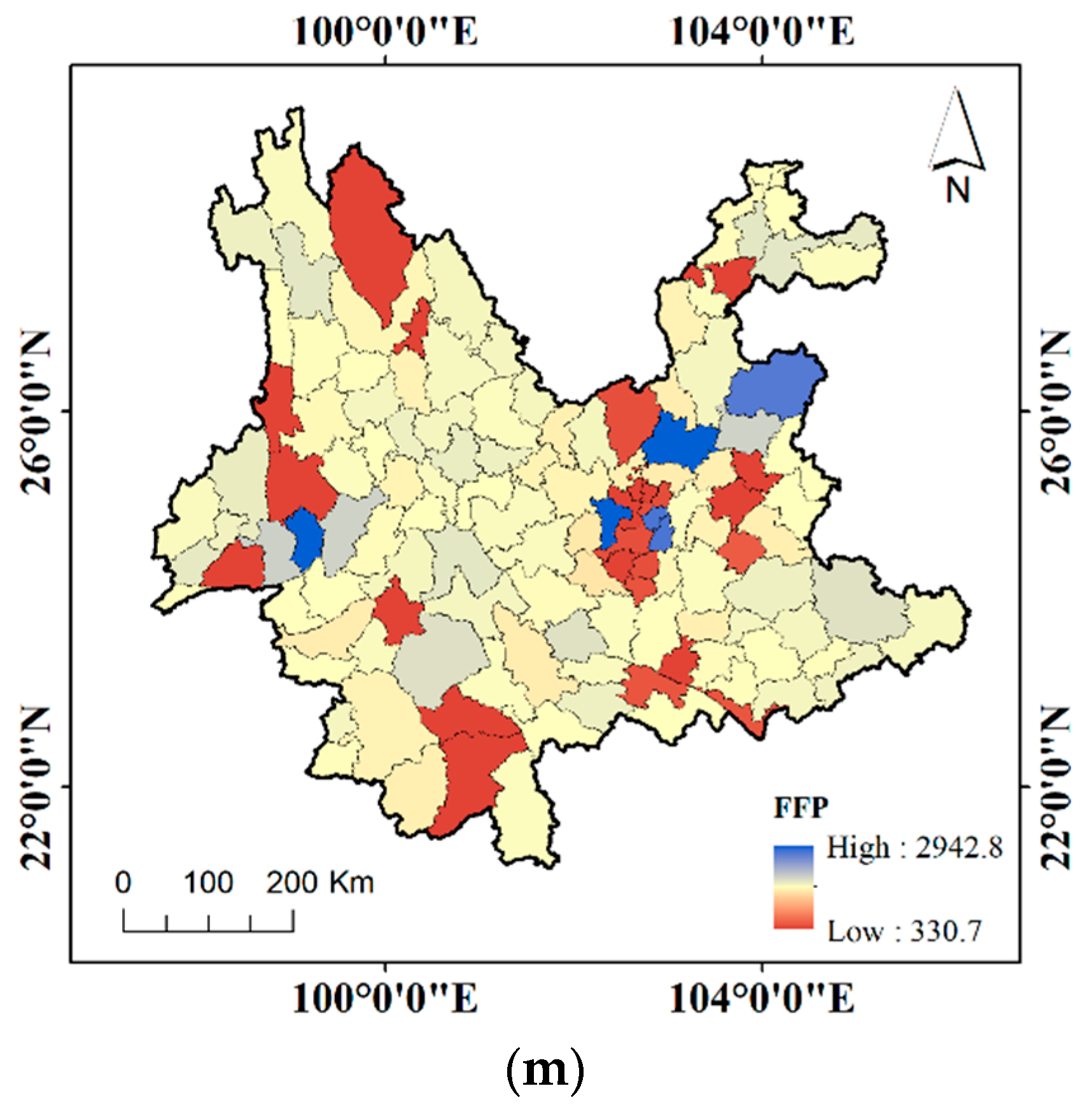
3.2. Flash Flood Risk Map Comparison

Based on the LR model and the LSSVM model with three kernels of LN, RBF and PL, the flood risk maps of Yunnan Province are generated in the GIS environment. As shown in Figure 5, the high-risk areas are mainly concentrated in the south-central region, accounting for 32% of the total area. Although LSSVM is not significantly better than LR in the training and testing, the risk distribution is significantly different. Figure 6 shows that the flash flood risk obtained by LSSVM is approximately a normal distribution, which is consistent with the previous study in Yunnan Province, China [32,33]. While the risk obtained by LR is a uniform distribution. Therefore, the flood risk maps obtained by LSSVM are more reliable than LR.
Many studies have utilized some statistical methods to conduct flash flood risk assessments in other areas. For example, Smith (2010) proposed the Flash Flood Potential Index (FFPI) model, considering slope, land use, soil texture and so forth. FFPI values from 1 to 10 correspond to the risk probability from the minimum to the maximum and has been tested in central Iowa, Colorado and upstate New York and Pennsylvania [34,35]. Based on the AHP and information entropy theory, Zeng et al. (2016) selected some relevant indicators (e.g., soil, slope, rainfall and flood control measures), utilized expert scoring method to explore their different weights and finally obtained the risk map of Yunnan Province [18]. In this study, the LSSVM method is firstly used for flash flood risk assessment. LSSVM can directly assess flood risk without setting factor weights. The contribution of each factor to flood risk is assessed by the correlation coefficient between factors and the flood risk, with a more significant advantage.
Figure 7 showed the correlation coefficient of each factor with the flash flood risk from LSSVM-RBF. The greater the correlation coefficient, the greater impact of this indicator on flash floods risk. Obviously, the correlation coefficient of CN is the largest, exceeding 0.5, followed by 7 indicators (DEM, SL, RD, FFP, TWI, 24-H-P, 3-H-P) between 0.1 and 0.5 and the remaining 5 indicators (AP, POP, SM, GDP, VC) are less than 0.1. Combined with the previous analysis, CN identifies the runoff generation capacity. DEM mainly responds to the topography of the study area and SL, RD and TWI all derived from DEM. Therefore, the flash flood risk of Yunnan Province is mainly affected by local runoff capacity, topography. Meanwhile, the correlation coefficient of FFP is 0.3, reflecting that positive man-made measures can largely prevent the occurrence of flash floods. However, compared with topographical factors, we found that the precipitation factor shows a relatively low correlation with the flash floods risk. This mainly because flash floods are caused by intensive rainfall but casualties are usually occurred and reported in low-lying areas. In addition, the effects of short-term precipitation (e.g., 24-H-P, 3-H-P) are greater than the annual precipitation. Our proposed model can concern all flash flood explanatory factors and give an accurate assessment for flash flood risk. In the future, we will further combine water depth and flow as a more reasonable indicator for flood assessment.

4. Conclusions

Flash floods have brought huge economic losses and casualties to China. An accurate flash flood risk assessment can identify flood-prone areas and give people enough time to prevent flood disasters in advance. In this study, LSSVM was selected to assess flash flood risk based on 13 explanatory factors. The main conclusions are as follows:
(1)
LSSVM can provide a more accurate risk assessment than LR and LSSVM with RBF kernel evaluates best.
(2)
The risk of flash flood in Yunnan Province is shown as a normal distribution. The highest risk areas are mainly concentrated in the central and western regions and the lowest risk areas are distributed in the northwest regions.
(3)
Flash floods are caused by the combination of various factors and the rank of various factors affecting flash floods is as follows: CN > DEM > SL > RD > FFP > TWI > 24-H-P > 3-H-P > AP > POP > SM > GDP > VC.
In conclusion, the paper utilized the LSSVM method to assess the flash flood risk for the first time and verifies that LSSVM with RBF kernel is suitable for assessing flash floods risk at large or medium scales. Since this method primarily collects explanatory factors and local flood records, where the explanatory factors are mainly derived from public datasets (remote sensing images and statistic bulletin) that can easily get for other areas. Thus, this method is feasible to apply in other regions by collecting local historical flood inventories. This method is highly dependent on data and lacks obvious physical mechanisms. Some problems, such as the shortage and uncertainty of flood inventories, limited the accuracy of model results. In particular, the historical flood record in this study was obtained through investigations by the authority of Yunnan Province, which limited the application of the research results to other regions. With the development of data mining technology, historical flood records from websites or media are desired to use for model development especially for data sparse areas in future works.

Author Contributions

All of the authors contributed to the conception and development of this manuscript. M.M. and G.Z. carried out the analysis and wrote the paper. C.L. designed the system framework and developed the project implementation plan. P.J. collected data and drew the study area map. D.W. participated in the results analysis. H.X., H.W. and Y.H. proposed many useful suggestions to improve its quality.

Funding

This research was funded by the projects of Application of remote sensing on water and soil conservation in Beijing and its demonstration (grant number Z161100001116102), Key technology on dynamic warning of flash flood in Henan Province (China) and its application(grant number HNSW-SHZH-2015-06), Study on infiltration mechanisms of special underlying surface in coalmine goal in Shanxi Province (China) and application of runoff generation and concentration theory(grant number ZNGZ2015-008_2), Research on spatial-temporal variable source runoff model and its mechanism(grant number JZ0145B2017) and National Natural Science Foundation of China (NSFC. General Projects: (grant number. 41471430)).

Acknowledgments

The authors are grateful to the editors and the anonymous reviewers for their insightful comments and suggestions, which helped to improve the manuscript.

Conflicts of Interest

The authors declare no conflicts of interest.

References

  1. Baker, V.R.; Kochel, R.C.; Patton, P.C. Flood Geomorphology; John Wiley and Sons: New York, NY, USA, 1987; ISBN 978-0-12-394846-5. [Google Scholar]
  2. Gruntfest, E.; Handmer, J. Coping with Flash Floods; Nato Science: Washington, DC, USA, 2001. [Google Scholar]
  3. Gourley, J.J.; Flamig, Z.L.; Vergara, H.; Kirstetteret, P.E.; Argyle, E.; Terti, G.; Erlingis, J.M.; Hong, Y.; Howard, K.W.; Arthur, A.; et al. The flooded locations and simulated hydrographs (FLASH) project: Improving the tools for flash flood monitoring and prediction across the United States. Bull. Am. Meteorol. Soc. 2016, 98, 361–372. [Google Scholar] [CrossRef]
  4. Mousavi, M.E.; Irish, J.L.; Frey, A.E.; Olivera, F.; Edge, B.L. Global warming and hurricanes: The potential impact of hurricane intensification and sea level rise on coastal flooding. Clim. Change 2011, 104, 575–597. [Google Scholar] [CrossRef]
  5. Creutin, J.D.; Borga, M.; Gruntfest, E.; Lutoff, C.; Zoccatelli, D.; Ruin, I. A space and time framework for analyzing human anticipation of flash floods. J. Hydrol. 2013, 482, 14–24. [Google Scholar] [CrossRef]
  6. Klijn, F.; Kreibich, H.; Moel, H.D.; Penning-Rowsell, E.C. Adaptive flood risk management planning based on a comprehensive flood risk conceptualization. Mitig. Adapt. Strateg. Glob. Chang. 2015, 20, 845–864. [Google Scholar] [CrossRef] [PubMed]
  7. Dutta, D.; Herath, S.; Musiake, K. A mathematical model for flood loss estimation. J. Hydrol. 2003, 277, 24–49. [Google Scholar] [CrossRef]
  8. Dottori, F.; Baldassarre, G.D.; Todini, E. Detailed data is welcome, but with a pinch of salt: Accuracy, precision, and uncertainty in flood inundation modeling. Water Resour. Res. 2014, 49, 6079–6085. [Google Scholar] [CrossRef]
  9. Alfieri, L.; Salamon, P.; Bianchi, A.; Neal, J.C.; Bates, P.; Feyen, L. Advances in pan-European flood hazard mapping. Hydrol. Process. 2014, 28, 4067–4077. [Google Scholar] [CrossRef]
  10. Sampson, C.C.; Smith, A.M.; Bates, P.D.; Neal, J.C.; Alfieri, L.; Freer, J.E. A high-resolution global flood hazard model. Water Resour. Res. 2015, 51, 7358–7381. [Google Scholar] [CrossRef] [Green Version]
  11. Mcmillan, H.K.; Brasington, J. Reduced complexity strategies for modelling urban floodplain inundation. Geomorphology 2007, 90, 226–243. [Google Scholar] [CrossRef]
  12. Bao, H.; Wang, L.; Zhang, K.; Li, Z. Application of a developed distributed hydrological model based on the mixed runoff generation model and 2D kinematic wave flow routing model for better flood forecasting. Atmos. Sci. Lett. 2017, 18, 284–293. [Google Scholar] [CrossRef] [Green Version]
  13. Huang, P.N.; Li, Z.J.; Li, Q.L.; Zhang, K.; Zhang, H.C. Application and comparison of coaxial correlation diagram and hydrological model for reconstructing flood series under human disturbance. J. Mt. Sci. 2016, 13, 1245–1264. [Google Scholar] [CrossRef]
  14. Ma, Z.; Shi, Z.; Zhou, Y.; Xu, J.; Yu, W.; Yang, Y. A spatial data mining algorithm for downscaling TMPA 3B43 V7 data over the Qinghai-Tibet Plateau with the effects of systematic anomalies removed. Remote Sens. Environ. 2017, 200, 378–395. [Google Scholar] [CrossRef]
  15. Tehrany, M.S.; Pradhan, B.; Mansor, S.; Ahmad, N. Flood susceptibility assessment using GIS-based support vector machine model with different kernel types. Catena 2015, 125, 91–101. [Google Scholar] [CrossRef]
  16. Kalteh, A.M. Improving forecasting accuracy of streamflow time series using least squares support vector machine coupled with data-preprocessing techniques. Water Resour. Manag. 2016, 30, 747–766. [Google Scholar] [CrossRef]
  17. Pradhan, B. Flood susceptible mapping and risk area delineation using logistic regression, GIS and remote sensing. J. Sp. Hydrol. 2010, 9, 1–18. [Google Scholar]
  18. Zeng, Z.; Tang, G.; Long, D.; Zeng, C.; Ma, M.; Hong, Y.; Xu, J. A cascading flash flood guidance system: Development and application in Yunnan Province, China. Nat. Hazards 2016, 84, 2071–2093. [Google Scholar] [CrossRef]
  19. Duan, C.C.; Zhu, Y.; You, W.H. Characteristic and formation cause of drought and flood in Yunnan province rainy season. Plateau Meteorol. 2007, 26, 402–408. [Google Scholar]
  20. Lindsay, J.B.; Rothwell, J.J.; Davies, H. Mapping outlet points used for watershed delineation onto DEM-derived stream networks. Water Resour. Res. 2008, 44, 370–380. [Google Scholar] [CrossRef]
  21. Zhao, G.; Pang, B.; Xu, Z.; Yue, J.; Tu, T. Mapping flood susceptibility in mountainous areas on a national scale in China. Sci. Total Environ. 2018, 615, 1133–1142. [Google Scholar] [CrossRef]
  22. Pettorelli, N.; Ryan, S.; Mueller, T.; Bunnefeld, N.; Jędrzejewska, B.; Lima, M.; Kausrud, K. The normalized difference vegetation index (NDVI): Unforeseen successes in animal ecology. Clim. Res. 2011, 46, 15–27. [Google Scholar] [CrossRef]
  23. Zeng, Z.; Tang, G.; Hong, Y.; Zeng, C.; Yang, Y. Development of an NRCS curve number global dataset using the latest geospatial remote sensing data for worldwide hydrologic applications. Remote Sens. Lett. 2017, 8, 528–536. [Google Scholar] [CrossRef]
  24. Sørensen, R.; Zinko, U.; Seibert, J. On the calculation of the topographic wetness index: Evaluation of different methods based on field observations. Hydrol. Earth Syst. Sci. 2005, 10, 101–112. [Google Scholar] [CrossRef]
  25. Abelen, S.; Seitz, F.; Abarca-del-Rio, R.; Güntner, A. Droughts and floods in the La Plata basin in soil moisture data and GRACE. Remote Sens. 2015, 7, 7324–7349. [Google Scholar] [CrossRef]
  26. Jongman, B.; Kreibich, H.; Apel, H.; Barredo, J.I.; Bates, P.D.; Feyen, L.; Ward, P.J. Comparative flood damage model assessment: Towards a European approach. Nat. Hazards Earth Syst. Sci. 2012, 12, 3733–3752. [Google Scholar] [CrossRef]
  27. Guo, L.; He, B.; Ma, M.; Chang, Q.; Li, Q.; Zhang, K.; Hong, Y. A comprehensive flash flood defense system in China: Overview, achievements, and outlook. Nat. Hazards 2018, 92, 1–14. [Google Scholar] [CrossRef]
  28. He, B.; Huang, X.; Ma, M.; Chang, Q.; Tu, Y.; Li, Q.; Hong, Y. Analysis of flash flood disaster characteristics in China from 2011 to 2015. Nat. Hazards 2017, 90, 1–14. [Google Scholar] [CrossRef]
  29. Dos Santos, G.S.; Luvizotto, L.G.J.; Mariani, V.C.; Dos Santos Coelho, L. Squares support vector machines with tuning based on chaotic differential evolution approach applied to the identification of a thermal process. Expert Syst. Appl. 2012, 39, 4805–4812. [Google Scholar] [CrossRef]
  30. Zhu, B.; Wei, Y. Carbon price forecasting with a novel hybrid ARIMA and least squares support vector machines methodology. Omega Intern. J. Manag. Sci. 2013, 41, 517–524. [Google Scholar] [CrossRef]
  31. Budimir, M.E.A.; Atkinson, P.M.; Lewis, H.G. A systematic review of landslide probability mapping using logistic regression. Landslides 2015, 12, 419–436. [Google Scholar] [CrossRef] [Green Version]
  32. He, J. Assessment and Regionalization of Drought Disaster Risk in Yunnan Province[D]; Yunnan University: Kunming, China, 2016. [Google Scholar]
  33. Wang, L.; Wang, S.; Wang, X.; Wang, F.; Fan, C. Risk zoning of drought disaster based on AHP and GIS in Yunnan province. Water Sav. Irrig. 2017, 10, 100–103, 106. [Google Scholar]
  34. Smith, G.E. Development of a Flash Flood Potential Index Using Physiographic Data Sets within a Geographic Information System. Ph.D. Thesis, The University of Utah, Salt Lake City, UT, USA, 2010. [Google Scholar]
  35. Minea, G. Assessment of the flash flood potential of Basca River Catchment (Romania) based on physiographic factors. Cent. Eur. J. Geosci. 2013, 5, 344–353. [Google Scholar] [CrossRef]
Figure 1. Location of the study area and the distribution of flash flood inventories (red for training and green for testing) from 2011 to 2015 in Yunnan Province, China.
Remotesensing 11 00170 g001
Figure 2. Explanatory factors affecting flash flood risk in this study.
Remotesensing 11 00170 g002
Figure 3. Explanatory factors of flash flood risk. (a) Annual Maximum 3 h Precipitation (b) Annual Maximum 24 h Precipitation; (c) Annual Precipitation (d) Digital Elevation Model; (e) Slope (f) River Density; (g) Vegetation Coverage (h) Curve Number; (i) Topographic Wetness Index (j) Soil Moisture; (k) Population (l) Gross Domestic Product; (m) Flash Flood Preventions.
Remotesensing 11 00170 g003aRemotesensing 11 00170 g003bRemotesensing 11 00170 g003c
Figure 4. ROC of four models in training (left) and testing (right). (Model 1: LSSVM + LN, model 2: LSSVM + RBF, model 3: LSSVM + PL, model 4: LR). (a) training (b) testing.
Remotesensing 11 00170 g004
Figure 5. Flood risk index distribution of different models. (Model 1: LSSVM + LN, model 2: LSSVM + RBF, model 3: LSSVM + PL, model 4: LR).
Remotesensing 11 00170 g005
Figure 6. Histogram of Flood index in different models. (Model 1: LSSVM + LN, model 2: LSSVM + RBF, model 3: LSSVM + PL, model 4: LR).
Remotesensing 11 00170 g006
Figure 7. The correlation coefficient between the flash flood risk and 13 indicators.
Remotesensing 11 00170 g007
Table 1. Factors, flood inventories and data sources.
NameSourceTime
AbbreviationMeaning
3-H-PAnnual maximum 3 h precipitationChina Meteorological Forcing Dataset2011–2015
24-H-PAnnual maximum 24 h precipitationChina Meteorological Forcing Dataset2011–2015
APAnnual precipitationChina Meteorological Forcing Dataset2011–2015
DEMDigital elevation modelShuttle Radar Topography Mission (SRTM)2000
SLSlopeShuttle Radar Topography Mission (SRTM)2000
RDRiver density Basic vector format dataset of China-
VCVegetation coverageMODIS products2011–2015
CNCurve number NRCS CN global dataset2011–2015
TWITopographic wetness indexShuttle Radar Topography Mission (SRTM)2000
SMSoil moisture ESA’s SMOS dataset2011–2015
PopPopulationData Center for Resources and Environmental Sciences Chinese Academy of Sciences (RESDC)2010
GDPGross domestic productData Center for Resources and Environmental Sciences Chinese Academy of Sciences (RESDC)2010
FFPFlash flood preventionsStatistic bulletin from the Ministry of Water Resources and local governments2012–2015
Table 2. Result of models in testing period.
IndexModel 1Model 2Model 3Model 4
Accuracy0.780.790.760.75
Precision0.810.820.790.76
Recall0.740.770.740.74
F-score0.780.790.760.75
Kappa0.560.590.530.50
Model 1: LSSVM + LN, model 2: LSSVM + RBF, model 3: LSSVM + PL, model 4: LR.

