Flood Mapping Using Multi-Source Remotely Sensed Data and Logistic Regression in the Heterogeneous Mountainous Regions in North Korea


1
Inter-Korean Forest Research Team, Division of Global Forestry, Department of Forest Policy and Economics, National Institute of Forest Science, 57 Hoegi-ro, Dongdaemun-gu, Seoul 02455, Korea
2
Department of Landscape Architecture, Graduate School, Sungkyunkwan University, Suwon 16419, Korea
*
Author to whom correspondence should be addressed.
Remote Sens. 2018, 10(7), 1036; https://doi.org/10.3390/rs10071036
Submission received: 4 June 2018
/
Revised: 15 June 2018
/
Accepted: 19 June 2018
/
Published: 1 July 2018
(This article belongs to the Special Issue Advances in Remote Sensing-based Disaster Monitoring and Assessment)
Abstract
:Flooding is extremely dangerous when a river overflows to inundate an urban area. From 1995 to 2016, North Korea (NK) experienced extensive damage to life and property almost every year due to a levee breach resulting from typhoons and heavy rainfall during the summer monsoon season. Recently, Hoeryeong City (2016) experienced heavy rain during Typhoon Lionrock, and the resulting flood killed and injured many people (68,900) and destroyed numerous buildings and settlements (11,600). The NK state media described it as the most significant national disaster since 1945. Thus, almost all annual repeat occurrences of floods in NK have had a severe impact, which makes it necessary to figure out the extent of floods to restore the damaged environment. However, this is difficult due to inaccessibility. Under such a situation, optical remote sensing (RS) data and radar RS data along with a logistic regression were utilized in this study to develop modeling for flood-damaged area delineation. High-resolution web-based satellite imagery was also interpreted to confirm the results of the study.
1. Introduction
Flooding is extremely dangerous when a river overflows to inundate an urban area. North Korea (NK) has suffered flood damage almost every year since 1995, so the region has come to be known as a natural disaster zone [1]. In particular, in 1995, 2007, and 2012, flash floods wreaked havoc on crop fields, human settlements, and infrastructure, thereby killing or displacing thousands of people. In these three years, the rate of deaths and injuries was 5.2 million, 900,000 and 298,000, respectively, and the number of destroyed buildings and settlements was 98,000, 240,000 and 87,000, respectively [1]. More recently, Raseon City (2015) and Hoeryeong City (2016) experienced typhoons (Goni and Lionrock, respectively) with heavy rainfall. Both areas are in North Hamgyeong Province, and the resulting floods killed and injured many people (11,000; 68,900) and destroyed numerous buildings and settlements (1000; 11,600) [2,3]. In particular, NK state media described the 2016 flood at Hoeryeong City as the biggest national disaster since 1945. Thus, it is necessary to develop a way to delineate Flood Damaged Areas (FDAs) in NK. However, it is difficult to conduct field investigations due to political divisions.
Under such a situation, remote sensing (RS) data can be used to delineate FDAs in NK. Several researchers have used optical RS data to assess floodplain delineations [4,5,6,7,8,9] and radar RS data, which is more immune to the presence of clouds, to detect flood inundations [8,10,11,12,13,14]. With these technologies, flooding can be monitored in inaccessible areas by ensuring repetitive coverage of the area of concern, especially before and after a disaster event.
A few studies have been conducted on NK flooding using RS data. Okamoto et al. [15] estimated the economic loss of a 1995 flood in terms of rice production in NK using optical RS data. Kim et al. [16] used Normalized Difference Vegetation Index (NDVI) values to elucidate the impact of the flood on the crop recovery conditions in agricultural areas in post-flood Japanese Earth Resources Satellite (JERS)-1 Optical Sensor (OPS) imagery. They also used JERS-1 Synthetic Aperture Radar (SAR) data as reference data to evaluate flooded crop fields in a classified land-cover map. However, they did not use satellite images taken near the day of the flood occurrence. Lim and Lee [17] found that the largest portion of NK flooding occurred in rice paddies with a low elevation. They also found that floods occur in NK even though the precipitation is similar to South Korea (SK), which does not experience floods. However, radar RS data were not used due to its unavailability.
Although radar RS data provides the benefits of data collection regardless of weather conditions, it is limited insofar as radar only recognizes a distributed target [10]. Thus, it is necessary to complement this data with water flow simulations using a Geographic Information System (GIS) to delineate the FDAs more accurately. Prior studies have used RS data and GIS integration models to detect and predict FDAs [8,10,11,12,14,18]. These models can be used in areas without field hydrologic data [14]. Therefore, they can be applied to study FDAs in otherwise-inaccessible areas of NK.
Recently, machine-learning techniques have been used for flood modeling and prediction. The popular methods in natural hazard modeling are Artificial Neural Networks (ANNs) [19,20,21,22], the Analytical Hierarchy Process (AHP) [23,24,25,26,27], Frequency Ratio (FR) [28,29,30,31,32,33,34,35,36], and Logistic Regression (LR) [8,14,30,34,37,38,39].
The LR model in GIS processing in this study is frequently used because of its straightforward and understandable concepts [28,33,39]. In addition, LR can explain the role of factors and it shows a strong prediction ability when compared to other machine-learning techniques [37]. Pradhan [8] progressed flood susceptible mapping and risk area delineation using LR, GIS and RS within Kelantan River in Malaysia. He used RADARSAT data for RS, and topographical map, geological map, hydrological map, Global Positioning System (GPS) data, land cover map, geological map, precipitation data, and Digital Elevation Model (DEM) for GIS data. His results showed that delineated flood prone areas can be performed at 1:25,000 scale which is comparable to some conventional flood hazard map scales. Chubey and Hathout [14] developed a geomatics-based approach for flood prediction method. They integrated RADARSAT and GIS modelling for estimating future Red River flood risk. They used LR with the following five independent variables: elevation; proximity to rivers and streams; proximity to roads; proximity to railways; and distance from already-flooded land. They insist that the methodology used in this research would be easily transferable to other areas, and may provide the basis for a viable alternative to conventional hydrologic-based flood prediction approaches. Nandi, Mandal, Wilson and Smith [38] progressed flood hazard mapping in Jamaica using principal component analysis and LR. They used fourteen factors, and of these factors, seven explained 65% of the variation in the data: elevation, slope angle, slope aspect, flow accumulation, a topographic wetness index, proximity to a stream network, and hydro-stratigraphic units.
Previously, modeling methods that used LR were tested for FDA delineation in an NK environment, finding limited value in this study. During heavy rainfall, debris flows occurred on terraced crop fields [40,41]. It is assumed that terraced crop fields in mountainous regions caused some errors. Therefore, based on these considerations we developed an FDA delineation model using multiple RS data with LR for heterogeneous mountainous regions in NK, where this model reflects the characteristics of the North Korean topography and identifies the critical factors for the NK flooding model. Ultimately, the study sought to provide basic information to mitigate flood risks in NK.
2. Materials and Methods
2.1. Study Area
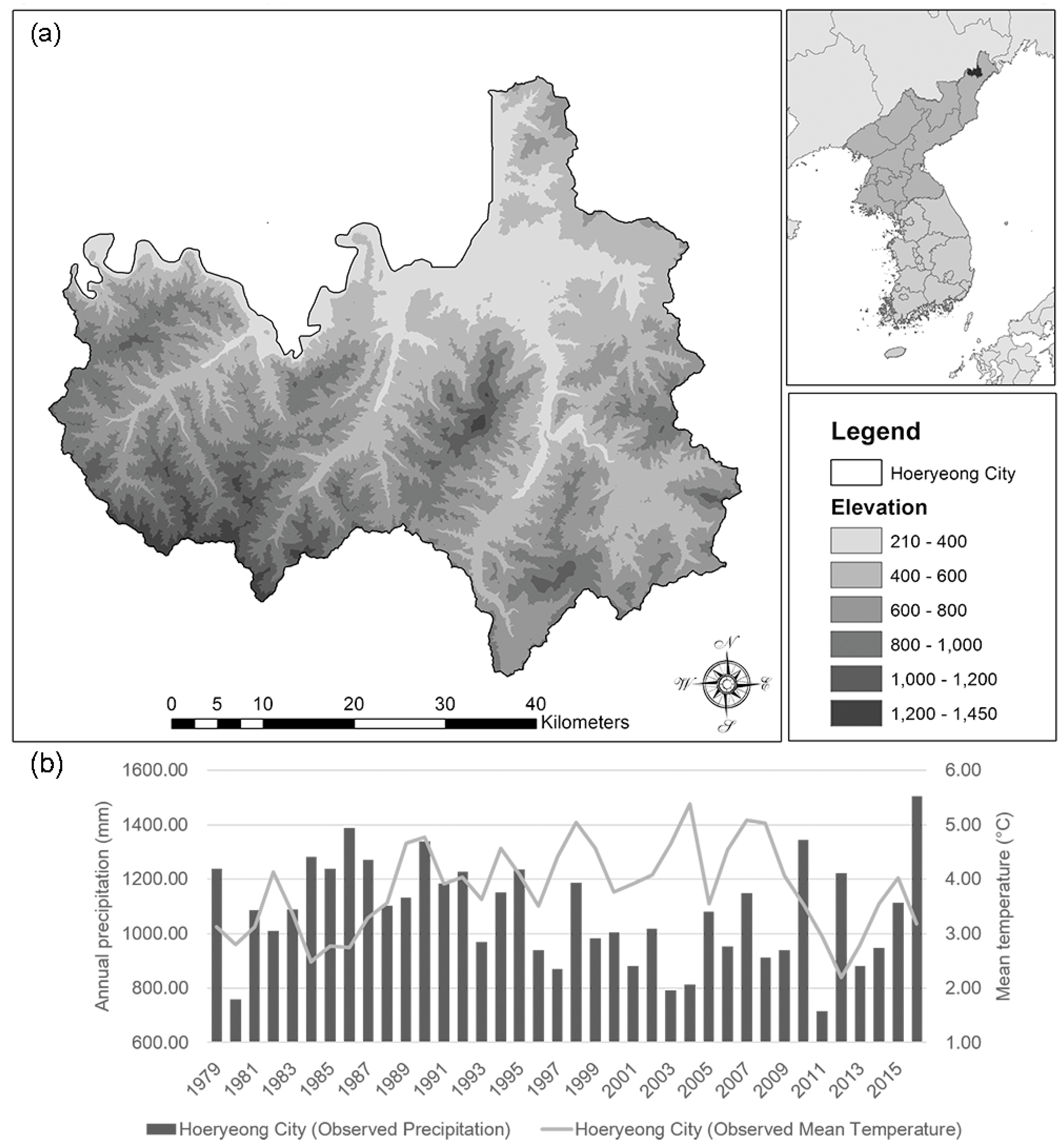
The study area is Hoeryeong City (42°26′N, 129°45′E) in northern NK. It is adjacent to the Tumen River, which flows between Hoeryeong City and the Jilin Province in China. Being a border city, it is a traffic trade center of North Hamgyeong Province in NK. Since NK’s great famines of the 1990s, food and other necessities have been imported from China by trade or smuggling. In addition, Hoeryeong City is a distribution and information communication channel in a closed NK society. Accordingly, there are many NK refugees in SK from the North Hamgyeong Province in NK, and most of these refugees are from Hoeryeong City (about 2000, 10%) [42]. Historically, Hoeryeong City has also been an important military hub area for national defense due to its location [43]. Its main industries are mining machinery and paper milling [44]. The study area is typically mountainous, with an elevation ranging from 210 m to 1450 m (Figure 1a). Hoeryeong City is surrounded by mountainous areas with an altitude of approximately 1000 m, and this excludes the Tumen River and adjacent villages, which are relatively low flat areas.
In terms of topography, the southeast portion of the Hoeryeong Basin is surrounded by mountains and the northwest is open to the Tumen River. The geology consists of Paleozoic sedimentary rock and granitic rock layers in the southeastern mountainous area whose elevation is equal to 500 m or more. The lower region of Hoeryeong City is composed of tertiary sedimentary rock layers. This region is used for agriculture since it is highly weathered and has relatively low elevations [45].
The study area has a continental climate with four distinct seasons: spring (March–May), summer (June–August), fall (September–November), and winter (December–February). The summer is hot and humid due to moist air coming from the Pacific Ocean. More than 60% of the annual precipitation occurs in the summer due to the East Asian monsoon winds [46]. The winter is dry and cold due to air masses coming from Siberia [47]. The annual mean precipitation and mean temperature from 1979 to 2016 were 1077 mm (±184 mm) and 3.8 °C (±0.8 °C), respectively (Figure 1b). Annual precipitation and temperature data were provided in the form of Climate Forecast System (CFS) Reanalysis data through Climate Engine (http://clim-engine.appspot.com/) by the National Weather Service (NWS) at the National Oceanic and Atmospheric Administration (NOAA) and the National Centers for Environmental Prediction (NCEP).
On 30 August 2016, the area experienced torrential rains brought by Typhoon Lionrock, which overflowed the Tumen River and brought huge amounts of water into the plains at least once. Consequently, North Korean state media distributed photographs of damage related to our study area. As previously mentioned, the media described the flood as the biggest national disaster since 1945, and casualties reached several hundred, including those dead and missing. Some 68,900 people had lost their homes, and there were also reports that “about 11,600 houses were destroyed, and that some 29,800 other houses suffered huge damage” [2]. Figure 2 shows images of the flood damage in Hoeryeong City.
2.2. Database Established
GIS databases were created to implement this research (Table 1). To delineate the FDA, Flood Inundated Areas (FIAs) were first derived using Sentinel-1 Single Look Complex (SLC) data obtained during pre-and post-flood instances. Radar data were obtained from the European Space Agency (ESA) Sentinels Scientific Data Hub (https://scihub.copernicus.eu/dhus/#/home). Then, digital topographic data of NK provided by the South Korean National Geographic Information Institute (NGII) were used to produce a digital elevation map, slope gradient map, landform map, a map of the Distance from the Nearest Stream (DNS), a flow accumulation map, and a flow direction map. They were used together with FIAs to delineate FDAs using binary LR. This model was made using the R software. A land use map was produced using Landsat 8 data gathered on 28 May 2016, obtained from the United States Geological Survey (USGS) Landsat homepage (http://earthexplorer.usgs.gov/). Level 1T data were processed using radiometric and geometric corrections. To confirm the results of the study, high-resolution Google Earth images were used. They were derived from GeoEye-1 data, which have 1.65 m spatial resolution, and they were taken on 16 October 2015, before flooding and on 15 September 2016, fourteen days after flooding.
2.3. Study Methods
This study consists of two parts. First, an LR model based on GIS was used to delineate FDAs and spatial characteristics of the FDAs were investigated. In the model, the FIA maps derived from the radar backscattering coefficient difference, elevation map, slope map, DNS map, land use map, landform map, flow accumulation map and flow direction map were used. After that, study results were confirmed via comparison with Google Earth images taken after the typhoon (Figure 3).
Delineation of Flood Damaged Areas
Delineation of FDAs consists of three parts. The first is FIA delineation from radar data and the second part is to generate an elevation map, slope map, DNS map, landform map, flow accumulation map and flow direction map from digital topographic data provided by NGII. In addition, land cover classification was performed to generate a land use map. The third part is FDA delineation using LR, which integrates the above data to generate FDA maps in this study.
First, FIA maps from radar processing were derived by comparing the backscattering coefficient of the Sentinel-1 data. The backscattering coefficient of a radar data is sensitive to floods; therefore, it can be used to determine the extent of flooding. Giacomelli, Mancini and Rosso [10] assessed flooded areas from ERS-1 PRI data with DEM data in Northern Italy. Their density-slicing method result showed that SAR data are sufficient for delineating flood areas. Brivio, Colombo, Maggi and Tomasoni [12] proposed an integration method for RS data and GIS to accurately map flooded areas in Regione Piemonte, Italy. They used ERS-1 SAR data and DEM data with visual interpretation, and thresholding techniques. Their proposed procedure was suitable for mapping flooded areas, even when satellite data were acquired some days after the event.
Before comparing backscattering coefficients, Sentinel-1 SLC data needs to be processed. Sentinel-1 SLC data has burst images, so a de-burst step was needed. Then, speckle filtering and terrain correction should be processed. All of these were processed using SNAP v. 3.0 by ESA, and ENVI 5.3.1.
There was only a VV (vertical transmit and vertical receive) polarization image of Hoeryeong City. Therefore, a VV polarization image was used for Hoeryeong City. To derive the backscattering coefficient, radar images should be converted to a decibel (dB) scale using logarithmic formation (Equation (1)).
here, σ0dB is the backscattering coefficient in a dB scale, and Intensity_VV is the original intensity value of the VV polarization image. To delineate FIAs, a backscattering coefficient difference (Δσ0) map was derived by the following:
where Δσ0 is the backscattering coefficient difference, σ0after flood is the backscattering coefficient after a flood, and σ0before flood is the backscattering coefficient before a flood.
The Δσ0 image was reclassified by the standard deviation. A standard deviation of-2 sigma or less was reclassified as an FIA. The slope map was then used to mask misclassified pixels in FIAs. Flooding occurred in SK in areas with a slope below 4° [48]. Since the topography of NK is similar to that of SK, areas with a slope of 4 degrees or more were masked.
However, this map could not represent FDAs clearly because SAR data can only recognize a distributed target [10]. Thus, the second part is to generate an elevation map, slope map, DNS map, landform map, flow accumulation map and flow direction map using digital topographic data from NGII. NK floods occur not only in the mainstream of river waterways, but also in middle- and upper-stream trajectories. Thus, the nearest-feature method of GRASS GIS 7.0.3 was used to delineate the nearest stream orders of FDAs and thereby determine whether flooding occurs in the mainstream or its branches. This information can be used to establish an improvement scheme [17]. The DEM was used to determine the stream order according to Hack’s stream ordering method [49,50] using GRASS GIS 7.0.3. The mainstream was classified as number 1, and all tributaries were classified sequentially using subsequent numbers (2, 3, and so on). To produce a DNS map, virtual points were generated for every pixel in the study area. After that, the distances between virtual points and the nearest stream were calculated using the “Near” function in ArcGIS. Then, point data were converted to grid data to generate a DNS map. Flow accumulation and flow direction maps were produced using Arc Hydro Tools 10.3 in ArcGIS.
A landform map was produced using Geomorphon [51]. It was used as an input variable in an LR model to investigate the landform of the FDAs. Tak [52] generated a landform map of the Korean Peninsula using Geomorphon. This system classifies landforms into 10 classes by determining cell patterns in relation to height comparisons between center cells and surrounding cells (Figure 4) [51]. The system calculates zenith and nadir angles to determine the correct principal compass directions among the eight possible directions. In this study, the landform map of NK was produced from 1:25,000 digital topographic maps from NGII using GRASS GIS 7.0.3.
To investigate the land use of the FDAs, a land use map was derived using the land cover classification with Landsat 8 data using ISODATA. The classification result accuracy was assessed using reference data which were selected by visual interpretation of the high-resolution Google Earth images. The land use map has four classes based on the Korea National Environment Information Network System’s (KNEINS) land cover classification scheme: crop field, forest, urban, and water. The classification result showed 98.7% in overall accuracy with a Kappa coefficient of 0.97, indicating a satisfactory level of accuracy.
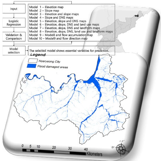
Lastly, an FDA delineation model was developed using an LR model. Ten models were tested to select the best model for FDA delineation. Model 1 used only an elevation map for modeling. Model 2 used a slope map, model 3 used elevation and slope maps, and model 4 used slope and DNS maps. Model 5 used elevation, slope and DNS maps, model 6 used elevation, slope, DNS and land use maps, and model 7 used elevation, slope, DNS and landform maps. Model 8 used elevation, slope, DNS, land use and landform maps, model 9 used elevation, slope, DNS, land use, landform and flow accumulation maps, and model 10 used elevation, slope, DNS, land use, landform, flow accumulation and flow direction maps (Figure 5). The R software was used to delineate FDAs.
The LR equation is as follows:
where p is the dependent variable (i.e., the probability that the event happened), is the intercept, x1 … xp are the independent variables, and … are the coefficients of the independent variables.
The coefficients are estimated using maximum likelihood estimation. The equation is as follows:
to find that maximize the logarithmic likelihood of Equation (4), the partial derivative of Equation 4 is taken with respect to , and the values that make it 0 are determined.
Independent variables were added to the model one at a time, using a statistical method to reduce the Akaike’s Information Criterion (AIC). AIC was developed by Akaike [53]. The AIC ranges from 0 to ∞, with smaller values indicating a better fit. AIC is often used to compare models across different samples. The model with the smaller AIC is considered the better fitting model. In this step, an elevation map, slope map, DNS map, landform map, land use map, flow accumulation map, and flow direction map were used in ten combinations to find the best-fitting model. After running several tests in this step, the most explainable independent variables (maps) were selected for the model of best fit. In addition, McFadden’s R2 [54] was calculated in order to test the goodness of fit. It can be viewed as a corresponding indictor of R2 of the linear regression model. Receiver Operating Characteristic (ROC) curve was used to assess the predictive ability of the model. The ROC curve was generated by plotting the true positive rate against the false positive rate at various threshold settings. If a model has an Area Under the Curve (AUC) closer to 1 and is greater than 0.5, this indicates that the model has good predictive ability [55]. In addition, the binomial deviance was compared between ten models to select the best-fitting model. The binomial deviance is as follows [56]:
if for all future observations, the D value is zero. If is always true, the value of D is infinite. Therefore, the smaller the D, the more accurate the model [56,57,58,59,60].
3. Results and Discussion
3.1. Flood Damaged Area Delineation
An FIA map was derived using radar processing. Backscattering coefficient values were decreased at sites A and B of Hoeryeong City. The average difference of the backscattering coefficient was −2.9 dB for site A and −5.2 dB for site B. These results provide clear evidence that the difference in the backscattering coefficients can be used to derive FIA maps. Therefore, it was used to produce FIA maps in this study.
FIA maps from radar processing and GIS data were integrated through a binary LR analysis to generate the FDA maps in this study. Model 7 exhibited the best fit for the data, with a low AIC (2722) and the lowest binomial deviance (820.23). In addition, model 7 showed the highest McFadden’s R2 (0.67) and AUC (0.97) among the ten models in the study area. This model had an AUC value of 0.97, indicating a good predictive ability (Table 2). After running several tests, the elevation map, slope map, DNS map and landform map were selected as independent variables in the LR.
Table 3 shows the LR coefficient for each variable. As shown in Table 3, the elevation, slope, and DNS have negative values. In addition, peak, ridge, and spur have large negative values. These are areas where common sense floods do not occur. This means that the developed model can reflect terrain properties when predicting FDAs.
Based on the model, coefficient values were applied to produce FDA maps. The equation is as follows:
where P is the spatial probability of a flood occurrence, ELEVATION is the elevation map, SLOPE is the slope map, DNS is the map of the distance from the nearest stream and LANDFORMC denotes the LR coefficient values listed in Table 3.
Finally, the result of the LR was generated in the range between 0 to 1 (100%). To select a threshold value, values from 0.5 to 0.9 were tested and compared with FIAs. After that, a threshold value of 0.7 showed the highest concordance rate by 89.1%. Therefore, this value was used to delineate the FDAs. Figure 6 shows an FDA map derived for the study area.
In this study, an FDA map from 30, August 2016, had an area of 106.63 km2 (7.81%) inundated in Hoeryeong City. The largest amount of flooding occurred in crop fields, followed by forests, and urbanized areas. The area of the crop field inundation was of 74.71 km2, and the area of the forest and urban inundation was 19.25 km2 and 12.67 km2, respectively. However, 57.95% of the entire urban area was flooded the most while 31.96% of crop fields and 1.78% of forest areas were inundated.
When we look at the landform of the FDAs, the flooding occurred mostly in flat areas (55.04 km2, 51.62%) followed by a valley (25.15 km2, 23.59%), footslope (20.07 km2, 18.82%), shoulder (3.20 km2, 3.00%), pit (1.14 km2, 1.07%), hollow (1.08 km2, 1.01%), and slope (0.95 km2, 0.89%). This result shows that the developed model reflected terrain properties when deriving the flooded area. However, when the DNS and landform were not used for predictions, the result showed some FDAs on unlikely landforms (e.g., hollows, spurs, peaks). During heavy rainfall, debris flows occurred on a terraced crop field [40,41] and this phenomenon can affect the backscattering coefficients of SAR data. Thus, floods can be detected on ridges, spurs or peaks. It is assumed that the terraced crop field on the mountainous region caused some errors. To correct these errors, we used the DNS and landform map to delineate FDAs in this study. In addition, we reduced some errors. The landform was found to be an important factor in delineating FDAs using a logical expression in the study area, which is different from other study results [8,14,38].
In Hoeryeong City, the FDAs near stream orders 1, 2, 3, 4, 5, 6, and 7 accounted for 5.44 km2 (5.11%), 34.19 km2 (32.06%), 25.83 km2 (24.22%), 20.26 km2 (19.00%), 16.41 km2 (15.39%), 3.66 km2 (3.43%), and 0.85 km2 (0.80%) of the inundation, respectively. The inundations occurred mainly in a lower-order stream (1 and 2; 37.17%) and middle-order stream (3, 4 and 5; 58.61%). Therefore, it is once again confirmed that the DNS is an important factor in delineating FDAs in NK [17].
Water was assumed to flow over the banks of the main river or lower stream in flat areas, and it was assumed that streambeds in the middle-stream channels in valleys and footslope areas were elevated by erosion materials transported from terraced crop fields [40,41,61].
After the collapse of the Soviet Union in 1989, NK could not receive food support from them. To solve the food shortage, the NK government began deforestation of steep slopes to make room for farms that would enhance agricultural output. In a 2004 report released by the South Korean government [62], 7.9% (972,000 ha) of NK’s total area (12,298,000 ha) was classified as deforested (i.e., as terraced crop fields). This condition makes land structures vulnerable to flooding and landslides in the summer monsoon season because land use changes can affect the occurrence of floods [63,64,65,66].
The riverbank drainage capacity was assumed to have been reduced due to the rise in the riverbed elevation, resulting from sediment carried and then deposited by heavy rainfall in NK monsoon events [40,42]. In 2016, the study area also experienced levee breaches that contributed to extreme flooding damage.
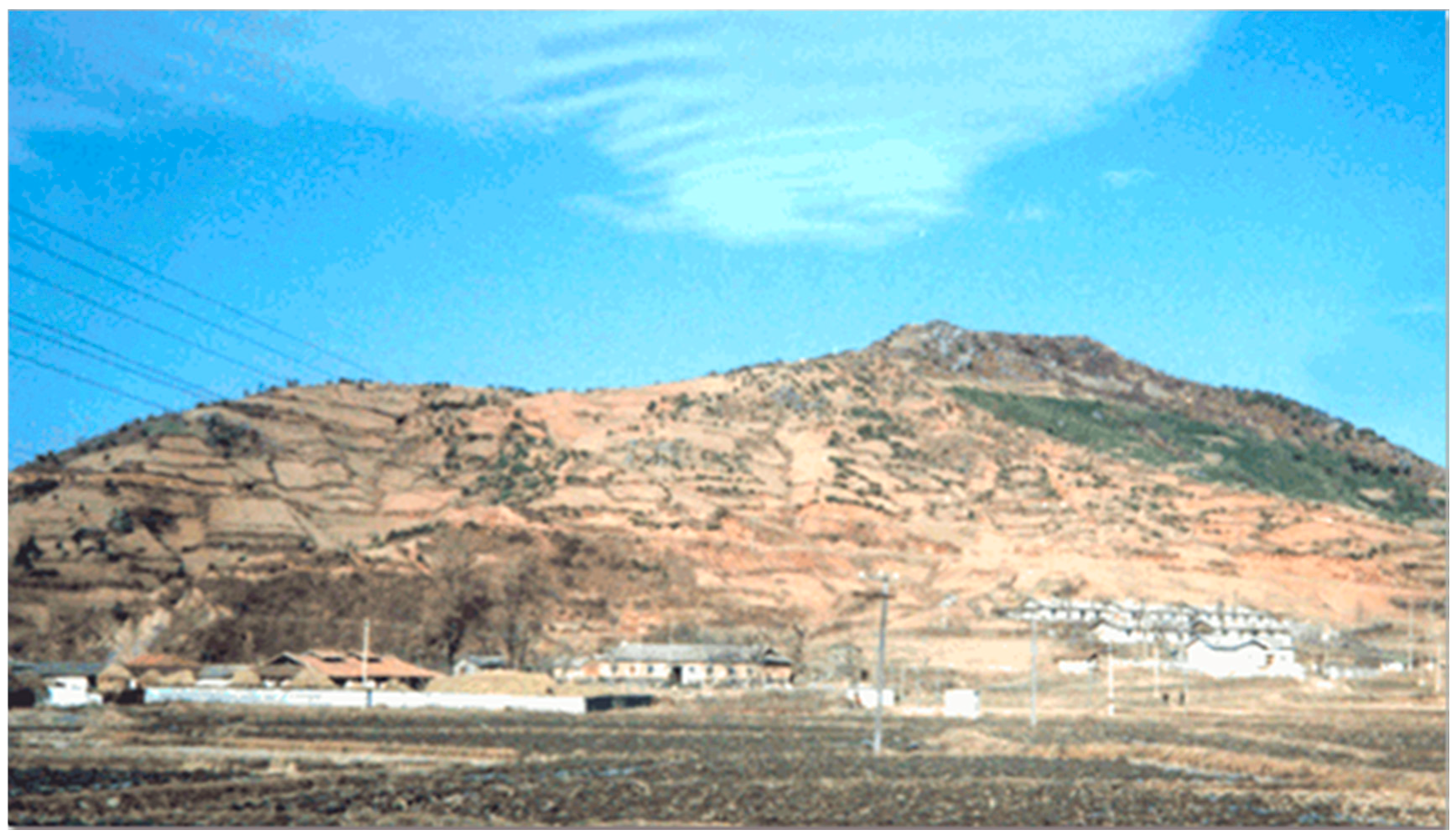
Based on all these findings (1) increased sediment deposits derived from upper streams contributed to a rise in riverbeds and a decrease in drainage capacity, and (2) levee breaches resulted in extreme flood damage within the study area. Thus, the transformation of mountain and hill forests to terraced crop fields in NK over the past years (Figure 7) has increased the risk of flood disasters.
3.2. Study Result Confirmation
To confirm the study results, the developed FDA delineation model was tested using the 1993 Paju City flood site in SK. A flood map of Paju City was provided by Water Resources Management Information System (WAMIS). There was a typhoon with heavy rainfall in Paju City; it caused a levee breach and 7.47 km2 of the test site were inundated [67]. Table 4 shows a comparison of the results from the FDA map from this study model and the flood map from WAMIS. Table 4 shows that the developed model had more than 88.5% overall accuracy with a Kappa coefficient of 0.8, indicating that the model has reasonable FDA delineation accuracy. As shown in the table, the model has reasonable FDA delineation accuracy.
High-resolution Google Earth images helped the authors overcome the limitations of not having any field observations. In the past, researchers have used aerial photographs to delineate FIAs or to confirm the results of their study [12,68]. Recently, high-resolution satellite imagery has been used as ground reference data [69]. To confirm the results of the study, a visual interpretation image was produced using high-resolution Google Earth images taken on 15 September 2016, fourteen days after flooding. It was overlaid with the FDA map derived from the model in this study (Figure 8). White lines show the FDA boundary visually interpreted by the authors, and the black lines show the FDA boundary from the study model. The comparison shows that 92.6% of both FDA maps are the same (Table 5).
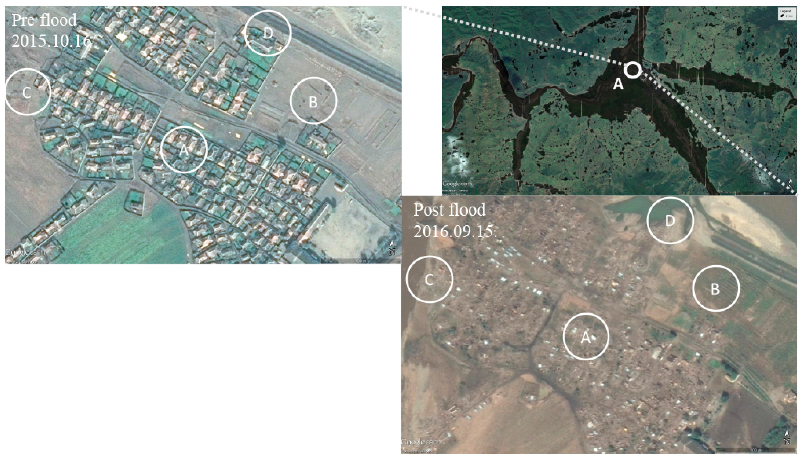
Figure 9 shows pre- and post-flood conditions around the main stream in the study area. Buildings were destroyed (Figure 9 Circle A) and crop fields were inundated (Figure 9 Circle B). According to the United Nations Resident Coordinator for Democratic people’s Republic of Korea (UNRCDPRK) team report, the level of the Tumen River rose between 6 and 12 meters on 30 August 2016 [61]. As illustrated in Figure 9, the river overflowed the levee (Circle C), causing a breach (Circle D). It is presumed that the levee breach resulted from the increased riverbed elevation caused by the deposition of erosion materials coming from terraced crop fields.
The UNRCDPRK team reported that 2700 houses were directly affected by the flood [61] in the survey area of Hoeryeong City. Our estimation of inundated housing units in the corresponding area showed that 2577 houses were directly affected, yielding a 95.4% compatibility rate with the field observation proffered by the UNRCDPRK team (Table 6). For the entirety of Hoeryeong City, the NK government announced that over 10,000 households were damaged (Figure 10) while our study estimated that 10,726 households were damaged (Table 6). Building data were derived by digital maps of NK provided by NGII. The maps were produced by visual interpretation using high-resolution satellite data. These comparisons demonstrate the validity of the study results.
4. Conclusions
This research investigated FDA mapping of Hoeryeong City, NK using multiple RS data and an LR machine-learning model. The results of the study were confirmed by a comparison with a visual interpretation of high-resolution web-based satellite images. The following conclusions were derived from this study:
- (1)
- On 30 August 2016, an area of 106.63 km2 (7.81%) in Hoeryeong City was inundated. Most floods occurred in flat areas adjacent to lower- and middle-order streams.
- (2)
- The DNS map and landform map developed in the model in this study are important factors for delineating FDAs because these two factors reflect NK topography, which is a heterogeneous mountainous region.
- (3)
- High-resolution web-based satellite imagery can be used as ground-truth data in inaccessible regions.
In conclusion, erosion materials coming from terraced crop fields during heavy rainfall were deposited in streambeds, increasing the elevation of the riverbed, reducing the stream drainage capacity, and causing levee breaches. The totality of these effects resulted in serious floods. Accordingly, the NK government should develop stream-drainage improvement measures to prevent flood damages caused by terraced crop fields and priority recovery areas need to be assessed to restore FDAs.
Author Contributions
J.L. and K.L. conceived and designed the experiments. J.L. performed the experiments, analyzed the data, and wrote the paper. All authors discussed and reviewed the manuscript.
Funding
Basic Research Project of the National Research Foundation of Korea (2013R1A1A2010007) and Samsung Academic Research: S-2012-0796-000-1
Conflicts of Interest
The authors declare no conflict of interest.
References
- Korea Ministry of Unification. Annual Rainfall Damages Status in North Korea. Available online: http://nkinfo.unikorea.go.kr/nkp/overview/nkOverview.do?sumryMenuId=SO322 (accessed on 24 January 2017).
- Kim, M.S.N. Korea Reeling from Flood Damage. Available online: http://english.chosun.com/site/data/html_dir/2016/09/19/2016091901010.html (accessed on 8 November 2016).
- Yonhap News Agency. (LEAD) 40 People Killed, 11,000 Affected N. Korean Floods. Available online: http://english.yonhapnews.co.kr/search1/2603000000.html?cid=AEN20150826010300315 (accessed on 14 October 2016).
- Barton, I.J.; Bathols, J.M. Monitoring Floods with AVHRR. Remote Sens. Environ. 1989, 30, 89–94. [Google Scholar] [CrossRef]
- Dhakal, A.S.; Amada, T.; Aniya, M.; Sharma, R.R. Detection of areas associated with flood and erosion caused by a heavy rainfall using multitemporal Landsat TM data. Photogramm. Eng. Remote Sens. 2002, 68, 233–239. [Google Scholar]
- Hudson, P.F.; Colditz, R.R. Flood delineation in a large and complex alluvial valley, lower Pánuco basin, Mexico. J. Hydrol. 2003, 280, 229–245. [Google Scholar] [CrossRef]
- Amini, J. A method for generating floodplain maps using ikonos images and dems. Int. J. Remote Sens. 2010, 31, 2441–2456. [Google Scholar] [CrossRef]
- Pradhan, B. Flood susceptible mapping and risk area delineation using logistic regression, GIS and remote sensing. J. Spat. Hydrol. 2009, 9, 1–18. [Google Scholar]
- Volpi, M.; Petropoulos, G.P.; Kanevski, M. Flooding extent cartography with Landsat TM imagery and regularized kernel Fisher’s discriminant analysis. Comput. Geosci. 2013, 57, 24–31. [Google Scholar] [CrossRef]
- Giacomelli, A.; Mancini, M.; Rosso, R. Assessment of flooded areas from ERS-1 PRI data: An application to the 1994 flood in Northern Italy. Phys. Chem. Earth 1995, 20, 469–474. [Google Scholar] [CrossRef]
- Townsend, P.A.; Walsh, S.J. Modeling floodplain inundation using an integrated GIS with radar and optical remote sensing. Geomorphology 1998, 21, 295–312. [Google Scholar] [CrossRef]
- Brivio, P.A.; Colombo, R.; Maggi, M.; Tomasoni, R. Integration of remote sensing data and GIS for accurate mapping of flooded areas. Int. J. Remote Sens. 2002, 23, 429–441. [Google Scholar] [CrossRef]
- Liu, Z.; Huang, F.; Li, L.; Wan, E. Dynamic monitoring and damage evaluation of flood in north-west Jilin with remote sensing. Int. J. Remote Sens. 2002, 23, 3669–3679. [Google Scholar] [CrossRef]
- Chubey, M.S.; Hathout, S. Integration of RADARSAT and GIS modelling for estimating future Red River flood risk. GeoJournal 2004, 59, 237–246. [Google Scholar] [CrossRef]
- Okamoto, K.; Yamakawa, S.; Kawashima, H. Estimation of flood damage to rice production in North Korea in 1995. Int. J. Remote Sens. 1998, 19, 365–371. [Google Scholar] [CrossRef]
- Kim, C.; Choi, J.; Joung, G. A Pilot Study on Environmental Evaluating and Estimation of the North Korea Flooded Area Using Spaceborne Scanner Data; The Korean Federation of Science and Technology Societies: Seoul, Korea, 1998; pp. 66–150. [Google Scholar]
- Lim, J.; Lee, K.S. Investigating flood susceptible areas in inaccessible regions using remote sensing and geographic information systems. Environ. Monit. Assess. 2017, 189, 96. [Google Scholar] [CrossRef] [PubMed]
- Mamat, R.; Mansor, S.B. Remote sensing and GIS for flood prediction. In Proceedings of the Twentieth Asian Conference of Remote Sensing, Hong Kong, China, 22–25 November 1999. [Google Scholar]
- Pradhan, B.; Buchroithner, M.F. Comparison and Validation of Landslide Susceptibility Maps Using an Artificial Neural Network Model for Three Test Areas in Malaysia. Environ. Eng. Geosci. 2010, 16, 107–126. [Google Scholar] [CrossRef]
- Kia, M.B.; Pirasteh, S.; Pradhan, B.; Mahmud, A.R.; Sulaiman, W.N.A.; Moradi, A. An artificial neural network model for flood simulation using GIS: Johor River Basin, Malaysia. Environ. Earth Sci. 2012, 67, 251–264. [Google Scholar] [CrossRef]
- Tiwari, M.K.; Chatterjee, C. Uncertainty assessment and ensemble flood forecasting using bootstrap based artificial neural networks (BANNs). J. Hydrol. 2010, 382, 20–33. [Google Scholar] [CrossRef]
- Pradhan, B.; Lee, S. Landslide susceptibility assessment and factor effect analysis: Backpropagation artificial neural networks and their comparison with frequency ratio and bivariate logistic regression modelling. Environ. Model. Softw. 2010, 25, 747–759. [Google Scholar] [CrossRef]
- Dandapat, K.; Panda, G.K. Flood vulnerability analysis and risk assessment using analytical hierarchy process. Model. Earth Syst. Environ. 2017, 3, 1627–1646. [Google Scholar] [CrossRef]
- Sar, N.; Chatterjee, S.; Das Adhikari, M. Integrated remote sensing and GIS based spatial modelling through analytical hierarchy process (AHP) for water logging hazard, vulnerability and risk assessment in Keleghai river basin, India. Model. Earth Syst. Environ. 2015, 1, 31. [Google Scholar] [CrossRef]
- Rozos, D.; Bathrellos, G.D.; Skillodimou, H.D. Comparison of the implementation of rock engineering system and analytic hierarchy process methods, upon landslide susceptibility mapping, using GIS: A case study from the Eastern Achaia County of Peloponnesus, Greece. Environ. Earth Sci. 2011, 63, 49–63. [Google Scholar] [CrossRef]
- Chen, Y.-R.; Yeh, C.-H.; Yu, B. Integrated application of the analytic hierarchy process and the geographic information system for flood risk assessment and flood plain management in Taiwan. Nat. Hazards 2011, 59, 1261–1276. [Google Scholar] [CrossRef]
- Yalcin, A. GIS-based landslide susceptibility mapping using analytical hierarchy process and bivariate statistics in Ardesen (Turkey): Comparisons of results and confirmations. CATENA 2008, 72, 1–12. [Google Scholar] [CrossRef]
- Samanta, R.K.; Bhunia, G.S.; Shit, P.K.; Pourghasemi, H.R. Flood susceptibility mapping using geospatial frequency ratio technique: A case study of Subarnarekha River Basin, India. Model. Earth Syst. Environ. 2018, 4, 395–408. [Google Scholar] [CrossRef]
- Shafapour Tehrany, M.; Shabani, F.; Neamah Jebur, M.; Hong, H.; Chen, W.; Xie, X. GIS-based spatial prediction of flood prone areas using standalone frequency ratio, logistic regression, weight of evidence and their ensemble techniques. Geomat. Nat. Hazards Risk 2017, 8, 1538–1561. [Google Scholar] [CrossRef] [Green Version]
- Youssef, A.M.; Pradhan, B.; Sefry, S.A. Flash flood susceptibility assessment in Jeddah city (Kingdom of Saudi Arabia) using bivariate and multivariate statistical models. Environ. Earth Sci. 2016, 75, 12. [Google Scholar] [CrossRef]
- Tehrany, M.S.; Pradhan, B.; Mansor, S.; Ahmad, N. Flood susceptibility assessment using GIS-based support vector machine model with different kernel types. CATENA 2015, 125, 91–101. [Google Scholar] [CrossRef]
- Tehrany, M.S.; Pradhan, B.; Jebur, M.N. Flood susceptibility analysis and its verification using a novel ensemble support vector machine and frequency ratio method. Stoch. Environ. Res. Risk Assess. 2015, 29, 1149–1165. [Google Scholar] [CrossRef]
- Tehrany, M.S.; Pradhan, B.; Jebur, M.N. Flood susceptibility mapping using a novel ensemble weights-of-evidence and support vector machine models in GIS. J. Hydrol. 2014, 512, 332–343. [Google Scholar] [CrossRef]
- Tehrany, M.S.; Pradhan, B.; Jebur, M.N. Spatial prediction of flood susceptible areas using rule based decision tree (DT) and a novel ensemble bivariate and multivariate statistical models in GIS. J. Hydrol. 2013, 504, 69–79. [Google Scholar] [CrossRef] [Green Version]
- Lee, M.J.; Kang, J.E.; Jeon, S. Application of frequency ratio model and validation for predictive flooded area susceptibility mapping using GIS. In Proceedings of the 2012 IEEE International Geoscience and Remote Sensing Symposium, Munich, Germany, 22–27 July 2012; pp. 895–898. [Google Scholar]
- Pradhan, B.; Mansor, S.; Pirasteh, S.; Buchroithner, M.F. Landslide hazard and risk analyses at a landslide prone catchment area using statistical based geospatial model. Int. J. Remote Sens. 2011, 32, 4075–4087. [Google Scholar] [CrossRef]
- Shafizadeh-Moghadam, H.; Valavi, R.; Shahabi, H.; Chapi, K.; Shirzadi, A. Novel forecasting approaches using combination of machine learning and statistical models for flood susceptibility mapping. J. Environ. Manag. 2018, 217, 1–11. [Google Scholar] [CrossRef] [PubMed]
- Nandi, A.; Mandal, A.; Wilson, M.; Smith, D. Flood hazard mapping in Jamaica using principal component analysis and logistic regression. Environ. Earth Sci. 2016, 75, 465. [Google Scholar] [CrossRef]
- Liao, X.; Carin, L. Migratory logistic regression for learning concept drift between two data sets with application to UXO sensing. IEEE Trans. Geosci. Remote Sens. 2009, 47, 1454–1466. [Google Scholar] [CrossRef]
- Lee, M.B.; Kim, N.S.; Cho, Y.C.; Cha, J.Y. Landform and Environment in Border Region of N. Korea and China. J. Korean Geogr. Soc. 2016, 51, 761–777. [Google Scholar]
- Myeong, S.; Kim, J.; Lim, M.; Hwang, S.; Son, G.; Ahn, J.; Gang, S.; Joo, G. A Study on Constructing a Cooperative System for South and North Koreas to Counteract Climate Change on the Korean Peninsula III; Korea Environment Institute: Seoul, Korea, 2013; pp. 68–79. [Google Scholar]
- Kwak, I.O. Spatial Structure and Function of Heoryong Market. Ph.D. Thesis, Korea University, Seoul, Korea, 2013. [Google Scholar]
- Shin, J.I. (Newly Written by Shin, Jeong Il) TaekRiJi—North Korea; Next Thinking: Goyang, Korea, 2012; pp. 30–36. [Google Scholar]
- Wikipedia. Hoeryong. Available online: https://en.wikipedia.org/wiki/Hoeryong (accessed on 14 October 2016).
- Lee, M.B.; Kim, N.S.; Kang, C.S.; Shin, K.H.; Choe, H.S.; Han, U. Estimation of soil loss due to cropland increase in Hoeryeung, Northeast Korea. J. Korean Assoc. Reg. Geogr. 2003, 9, 373–384. [Google Scholar]
- Gunjal, K.; Goodbody, S.; Hollema, S.; Ghoos, K.; Wanmali, S.; Krishnamurthy, K.; Turano, E. FAO/WFP Crop and Food Security Assessment Mission to the Democratic People's Republic of Korea; Food and Agriculture Organization of the United Nations/World Food Programme: Rome, Italy, 2013; p. 11. [Google Scholar]
- Wikipedia. North Korea. Available online: https://en.wikipedia.org/wiki/North_Korea#Climate (accessed on 8 June 2016).
- Kim, S.J.; Suh, K.; Kim, S.M.; Lee, K.D.; Jang, M.W. Mapping of inundation vulnerability using geomorphic characteristics of flood-damaged farmlands—A case study of Jinju City. J. Korean Soc. Rural Plan. 2013, 19, 51–59. [Google Scholar] [CrossRef]
- Jasiewicz, J. r. stream.order. Available online: https://grass.osgeo.org/grass70/manuals/addons/r.stream.order.html (accessed on 14 April 2016).
- Hack, J.T. Studies of Longitudinal Stream Profiles in Virginia and Maryland; US Government Printing Office: Washington, DC, USA, 1957; pp. 45–97.
- Jasiewicz, J.; Stepinski, T.F. Geomorphons—A pattern recognition approach to classification and mapping of landforms. Geomorphology 2013, 182, 147–156. [Google Scholar] [CrossRef]
- Tak, H.M. Optimal Variable Establishment for Using Geomorphons in Korean Peninsula. J. Korean Geomorphol. Assoc. 2014, 21, 165–183. [Google Scholar]
- Akaike, H. A new look at the statistical model identification. IEEE Trans. Automat. Control 1974, 19, 716–723. [Google Scholar] [CrossRef]
- McFadden, D. Conditional logit analysis of qualitative choice behavior. In Frontiers in Econometrics; Zarembka, P., Ed.; Wiley: New York, NY, USA, 1973; pp. 105–142. [Google Scholar]
- Alice, M. How to Perform a Logistic Regression in R. Available online: https://www.r-bloggers.com/how-to-perform-a-logistic-regression-in-r/ (accessed on 6 February 2017).
- Kwon, J.M. Data Science to Follow and Learn; Jpub: Seoul, Korea, 2017. [Google Scholar]
- Yang, M.; Xu, L.; White, M.; Schuurmans, D.; Yu, Y.-L. Relaxed clipping: A global training method for robust regression and classification. In Proceedings of the Advances in Neural Information Processing Systems, Vancouver, BC, Canada, 6–9 December; pp. 2532–2540.
- Rodríguez, G. Generalized Linear Models. Available online: http://data.princeton.edu/wws509/notes/a2s4.html (accessed on 8 June 2018).
- Hastie, T.; Tibshirani, R.; Friedman, J. The Elements of Statistical Learning, 2nd ed.; Springer: New York, NY, USA, 2009. [Google Scholar]
- McCullagh, P.; Nelder, J.A. Generalized Linear Models, 2nd ed.; Champman and Hall: London, UK, 1989. [Google Scholar]
- UNRCDPRK. Joint Assessment North Hamgyong Floods 2016; UN Resident Coordinator for DPR Korea: Pyeongyang, Korea, 2016; pp. 2–30. [Google Scholar]
- Lee, S.H. Situation of Degraded Forest Land in DPRK and Strategies for Forestry Cooperation between South and North Korea. J. Agric. Life Sci. 2004, 38, 101–113. [Google Scholar]
- Lin, B.; Chen, X.; Yao, H.; Chen, Y.; Liu, M.; Gao, L.; James, A. Analyses of landuse change impacts on catchment runoff using different time indicators based on SWAT model. Ecol. Indic. 2015, 58, 55–63. [Google Scholar] [CrossRef]
- Ye, W.S.; Lee, H.S.; Lee, K.S. Application of the GIS in the Hydrologic Effects Caused by the Second Collective Facility Area Development in Mt. Kyeryong National Park. J. Environ. Impact Assess. 1994, 3, 57–68. [Google Scholar]
- Guo, H.; Hu, Q.; Jiang, T. Annual and seasonal streamflow responses to climate and land-cover changes in the Poyang Lake basin, China. J. Hydrol. 2008, 355, 106–122. [Google Scholar] [CrossRef]
- Shankman, D.; Liang, Q. Landscape Changes and Increasing Flood Frequency in China’s Poyang Lake Region. Prof. Geogr. 2003, 55, 434–445. [Google Scholar] [CrossRef]
- Water Resources Management Information System. Flood Record. Available online: http://www.wamis.go.kr/WKF/WKF_FDDATIQ_LST.aspx?code=10536 (accessed on 29 June 2017).
- Oberstadler, R.; HÖNsch, H.; Huth, D. Assessment of the mapping capabilities of ERS-1 SAR data for flood mapping: A case study in Germany. Hydrol. Process. 1997, 11, 1415–1425. [Google Scholar] [CrossRef]
- Nakmuenwai, P.; Yamazaki, F.; Liu, W. Automated Extraction of Inundated Areas from Multi-Temporal Dual-Polarization RADARSAT-2 Images of the 2011 Central Thailand Flood. Remote Sens. 2017, 9, 78. [Google Scholar] [CrossRef]
Figure 1.
Elevation map and annual precipitation and annual mean temperature in the study area. (a) Elevation map (unit: m), (b) annual precipitation (mm) and annual mean temperature (°C).
Figure 1.
Elevation map and annual precipitation and annual mean temperature in the study area. (a) Elevation map (unit: m), (b) annual precipitation (mm) and annual mean temperature (°C).

Figure 2.
Flood damage in Hoeryeong City in August of 2016 (http://kp.one.un.org/content/unct/dprk/en/home/emergency-response/floods-2016.html, http://www.bbc.com/news/world-asia-37335857).
Figure 2.
Flood damage in Hoeryeong City in August of 2016 (http://kp.one.un.org/content/unct/dprk/en/home/emergency-response/floods-2016.html, http://www.bbc.com/news/world-asia-37335857).

Figure 3.
Flow chart of this study. DNS: distance from the nearest stream, FDA: flood damaged area, FIA: flood inundated area, SLC: single look complex, UNRCDPRK: United Nations resident coordinator for Democratic People ’s Republic of Korea.
Figure 3.
Flow chart of this study. DNS: distance from the nearest stream, FDA: flood damaged area, FIA: flood inundated area, SLC: single look complex, UNRCDPRK: United Nations resident coordinator for Democratic People ’s Republic of Korea.

Figure 4.
Landform classes in the Geomorphon model [51].
Figure 4.
Landform classes in the Geomorphon model [51].

Figure 5.
Algorithmic flow diagram of logistic regression.

Figure 6.
Flood-damaged area map of the study area.

Figure 7.
Terraced crop fields in North Korea (Source: http://www.forest.go.kr/newkfsweb/html/HtmlPage.do?pg=/partic/partic_1104_con02.html&mn=KFS_02_08_06_03_04).
Figure 7.
Terraced crop fields in North Korea (Source: http://www.forest.go.kr/newkfsweb/html/HtmlPage.do?pg=/partic/partic_1104_con02.html&mn=KFS_02_08_06_03_04).

Figure 8.
FDA map confirmation through a visual interpretation using Google Earth image.

Figure 9.
High-resolution Google Earth images of the study area.

Figure 10.
Flood-damaged residential houses in the study area (source: http://kp.one.un.org/content/unct/dprk/en/home/emergency-response/floods-2016.html).
Figure 10.
Flood-damaged residential houses in the study area (source: http://kp.one.un.org/content/unct/dprk/en/home/emergency-response/floods-2016.html).


Table 1.
Databases in this study. DNS: distance from the nearest stream, ESA: European space agency, GIS: geographic information system, NGII: national geographic information institute, RS: remote sensing, USGS: United States geological survey.
Table 1.
Databases in this study. DNS: distance from the nearest stream, ESA: European space agency, GIS: geographic information system, NGII: national geographic information institute, RS: remote sensing, USGS: United States geological survey.
| Data | Period or Year | Spatial Resolution | Source | ||
|---|---|---|---|---|---|
| RS | Optical | Landsat 8 | 28 May 2016 | 30 m | USGS |
| GeoEye-1 | 16 October 2015 15 September 2016 | 1.65 m | Google Earth | ||
| Radar | Sentinel-1 | 6 August 2016 30 August 2016 | Range 5 m Azimuth 20 m | ESA | |
| GIS | Elevation map | 1:25,000 | NGII Digital topographic data | ||
| Slope map | |||||
| DNS map | |||||
| Landform map | |||||
| Flow accumulation map | |||||
| Flow direction map | |||||
Table 2.
Logistic regression model comparison. AIC: Akaike’s information criterion, AUC: area under curve.
Table 2.
Logistic regression model comparison. AIC: Akaike’s information criterion, AUC: area under curve.
| Model No. | AIC | McFadden’s R2 | AUC | Binomial Deviance |
|---|---|---|---|---|
| Model 1 | 5594 | 0.27 | 0.87 | 1860.31 |
| Model 2 | 3635 | 0.55 | 0.94 | 1118.90 |
| Model 3 | 3452 | 0.58 | 0.96 | 1028.13 |
| Model 4 | 3542 | 0.56 | 0.95 | 1089.82 |
| Model 5 | 3408 | 0.58 | 0.96 | 1022.68 |
| Model 6 | 3391 | 0.58 | 0.96 | 1016.07 |
| Model 7 | 2722 | 0.67 | 0.97 | 820.23 |
| Model 8 | 2705 | 0.67 | 0.97 | 821.65 |
| Model 9 | 2706 | 0.67 | 0.97 | 821.94 |
| Model 10 | 2705 | 0.67 | 0.97 | 822.93 |
Table 3.
Logistic regression coefficients.
| Coefficients of Logistic Regression | |
|---|---|
| (Intercept) | 2.840 |
| ELEVATION | −4.254 × 10⁻⁴ |
| SLOPE | −0.325 |
| DNS | −6.535 × 10⁻⁴ |
| LANDFORM@Flat | 0 |
| LANDFORM@Peak | −18.170 |
| LANDFORM@Ridge | −4.598 |
| LANDFORM@Shoulder | −0.024 |
| LANDFORM@Spur | −3.164 |
| LANDFORM@Slope | −1.540 |
| LANDFORM@Hollow | −1.315 |
| LANDFORM@Footslope | 0.115 |
| LANDFORM@Valley | −0.025 |
| LANDFORM@Pit | 0.017 |
Table 4.
Comparison of results from flood map model and official flood map.
| Observed Model | Flood (km2) | No Flood (km2) | Total (km2) | User Accuracy (%) |
|---|---|---|---|---|
| Flood (km2) | 6.88 | 0.86 | 7.74 | 89.0 |
| No flood (km2) | 0.59 | 4.22 | 4.81 | 87.8 |
| Total (km2) | 7.47 | 5.08 | 12.55 | |
| Producer accuracy (%) | 92.2 | 83.2 | ||
| Kappa: 0.8 Overall accuracy: 88.5 | ||||
Table 5.
Comparison of FDA maps for verification via Google Earth image.
| Area of FDA-Visual Interpretation | Area of FDA-Model | Matching Ratio |
|---|---|---|
| 35.5 km2 | 38.3 km2 | 92.6% |
Table 6.
Comparison of damaged buildings in the study area.
| UNCDPRK Report NK Government | Study Results | |
|---|---|---|
| Part of Hoeryeong City | 2700 (UNCDPRK) | 2577 |
| Hoeryeong City | >10,000 (NK) | 10,726 |
© 2018 by the authors. Licensee MDPI, Basel, Switzerland. This article is an open access article distributed under the terms and conditions of the Creative Commons Attribution (CC BY) license (http://creativecommons.org/licenses/by/4.0/).
Share and Cite
MDPI and ACS Style
Lim, J.; Lee, K.-s. Flood Mapping Using Multi-Source Remotely Sensed Data and Logistic Regression in the Heterogeneous Mountainous Regions in North Korea. Remote Sens. 2018, 10, 1036. https://doi.org/10.3390/rs10071036
AMA Style
Lim J, Lee K-s. Flood Mapping Using Multi-Source Remotely Sensed Data and Logistic Regression in the Heterogeneous Mountainous Regions in North Korea. Remote Sensing. 2018; 10(7):1036. https://doi.org/10.3390/rs10071036
Chicago/Turabian StyleLim, Joongbin, and Kyoo-seock Lee. 2018. "Flood Mapping Using Multi-Source Remotely Sensed Data and Logistic Regression in the Heterogeneous Mountainous Regions in North Korea" Remote Sensing 10, no. 7: 1036. https://doi.org/10.3390/rs10071036
Note that from the first issue of 2016, this journal uses article numbers instead of page numbers. See further details here.