Estimation of Usable Area of Flat-Roof Residential Buildings Using Topographic Data with Machine Learning Methods

Abstract

The real estate appraisal largely consists of estimating the property’s value based on the transaction prices of similar buildings with the usable area being one of the main comparative units. A Polish appraiser finds data mentioned in the Price and Value Register (PVR). However, one of the authors’ previous studies indicated that the PVR contained highly incomplete information on usable area of residential buildings rendering it impractical for real estate appraisal purposes. Here, we propose a machine learning method to estimate the usable area of flat-roof residential buildings based on Light Detection and Ranging (LiDAR) data as well as the Database of Topographic Objects (BDOT10k). First, we train models with different architectures on the exact project data of residential buildings available online, obtained mostly from the design offices Lipińscy and Archon. Then, we apply trained algorithms on available residential building in Koszalin, Poland, using BDOT10k and LoD1 standard LiDAR data, and compare the results with usable area reported in PVR. Results show that the usable area of flat-roof houses without garages and extensions can be calculated with great accuracy up to 4%, while for more complex flat-roof buildings-up to 4–10%, depending on how detailed data are available. The model may be used by real estate appraisers to approximate the unknown usable area of residential buildings with known transaction prices, and as such increase the number of properties that can be compared to the evaluated real estate. To estimate the usable area of buildings with more complex roofs, a higher standard of LiDAR data is needed.

1. Introduction

This work is a continuation of previous studies of one of the authors [1,2,3] on the completeness of data contained in the Polish Price and Value Register (PVR). It constitutes an element of Land and Building Register [4], and is an important source of data on real estate [5,6,7] used by real estate appraisers to estimate values of properties. PVR also plays a significant role in the real estate management, spatial policy, sustainable development policy, and tax system [8,9,10,11,12,13,14,15,16,17,18]. PVR data have become a subject of abundant research indicating its incompleteness or low quality [5,19,20,21,22]. The real estate appraisal largely consists of estimating the property’s value based on the transaction prices of similar buildings. A lack of data is the main reason for which a certified real estate appraiser must reject a specific transaction, and, considering a small number of transactions on the local market, real estate appraisal becomes problematic.

One of the authors analyzed 829 transactions in PVR in communes of Koszalin and Kołobrzeg districts in years 2010–2017, and found that data incompleteness is especially abundant in the case of parcels with residential buildings located on them. Data on transaction date, real estate location, plot size, and ownership type, were fully available. Information on the construction material of building walls and number of stories occurred in PVR in 63% cases, while, with regards to the construction year, was around 40%. Even lower availability characterizes data on the usable area, which PVR provided in only around 30% of transactions. Therefore, the studied register is not very useful in terms of the completeness of data for real estate evaluation, mainly due to the lack of information about the building usable area, which is mainly taken into account when assessing whether the building is similar to the one being evaluated by the appraiser.

The aim of this paper is to propose methods of estimating the usable area of residential buildings using Light Detection and Ranging (LiDAR) data as well as the Database of Topographic Objects (BDOT10k). A successful method may overcome limitations of PVR, and increase the number of available similar buildings needed for real estate appraisal in the given area. This method is not intended to replace the standard interior measurements of usable area, but to give an accurate estimation when only limited topographic data on the building are available. The accuracy of usable area estimation by different methods should be checked by applying them to the existing single-family houses with known usable areas. This step, however, is complicated by the fact that Polish law lacks consistent rules on how to calculate this property of buildings and premises.

Usable area definitions differ between currently binding Polish acts [23], and on the purpose of calculating the quantity. Therefore, various definitions can be found in the Act on Local Taxes and Charges [24], Act On Tax On Inheritance And Donations [25], Tenants’ Rights, Municipal Housing Stock and the Civil Code Amendment Act [26], Regulation of the Minister of Justice on the Establishment and Maintenance of Land and Mortgage Registers in an IT System [27], Polish Standards (PSs), and international standards. The data on usable area contained in PVR, concerning both buildings and premises, should be consistent [22] with the definition from the act on tenants’ rights, which is the following: “area of all the spaces in a building, in particular, the rooms, kitchens, pantries, lobbies, alcoves, halls, corridors, bathrooms and other rooms used for residential and housekeeping needs of the tenant, whatever their actual purpose or way of use; the usable area does not include the area of balconies, terraces, loggias, entresols, wardrobes, recessed wall cubbies, laundry rooms, drying rooms, baby carriage rooms, attics, cellars, and fuel storage rooms” [26].

The regulations concerning the real estate appraisal, in the context of detailed rules regarding how to calculate the usable area, mainly refer back to PSs, which were written by the Polish Commitee of Standarization and introduced by the Normalization Act of 3 April 1993 [28]. According to this act, application of a PS was voluntary; however, it could be made obligatory by the minister regulation or if a PS was mentioned in any act explicitly. Using a PS became voluntary without an exception with the Normalization Act of 12 September 2002 [29]. Since 1971, a standard PN-B-02365:1970 [30] was in power, and was commonly used to calculate the usable area [31]. In 1998, it was replaced by PN-ISO 9836:1997 [32], which was introduced as an identical standard with the international one, ISO 9836:1992 [33].

Both standards indicate that, when calculating the usable area, construction and partition walls, and structural columns should not be included, and measurement precision should be within 0.01 m. However, exhibited differences, presented in

Table 1. The differences between PN-B-02365:1970 and PN-ISO 9836:1997 in usable area measurement rules. Source: [30,32].

	PN-B-02365:1970	PN-ISO 9836:1997
state of walls during measurement	unplastered *	plastered
measuring height	1 m above floor level	at floor level
niches	included if over 0.1 m${}^2$	not included
wall protrusions	deducted if over 0.1 m${}^2$	not deducted
	if $H>2.2$ m—included in 100%	if $H>=1.9$ m—included in 100%
room height (H)	if $1.4<=H<=2.2$ m—included in 50%	if $H<1.9$ m—not included
	if $H<1.4$ m—not included
calculation precision	0.1 m${}^2$	0.01 m${}^2$
exterior areas, unclosed from all sides,
available from a given room	not included	included, indicated separately
e.g., balconies, terraces, loggias
internal staircase	not included	included

* if walls are plastered, a correction has to be made, assuming that external lining is 3 cm thick, internal one—2 cm thick.

, result in discrepancies within few percent [23,31].

Starting from 29 April 2012, when calculating the usable area of single-family houses and premises, the use of PN-ISO 9836:1997 became mandatory with the Regulation of the Minister of Transport, Construction and Maritime Economy of 25 April 2012 on Detailed Scope and Form of a Construction Project [34], with two additional rules, “(1) a premises is a self-contained housing unit composed of a room or rooms separated with permanent walls from the rest of the building, allocated for a people’s continuous stay, with which auxiliary rooms serve their housing needs, (2) rooms or their parts with a height equal to, or greater than, 2.20 m shall be included in the calculation of usable area in 100%, with a height from 1.40 m to 2.20 m—in 50%, while with a height of less than 1.40 m shall be omitted” [34]. An important consequence of the first rule is ignoring partition walls, unlike the previous standards. As such, until 1999, usable areas were calculated using PN-B-02365:1970, from 1999 to 2012 both standards were applicable, and, finally, in 2012, PN-ISO 9836:1997 with two additional rules became obligatory for newly-built single-family houses and premises. To account for these changes, this study needs to take into account both standards as well as the 1997 standard with two rules (written as PN-ISO 9836:1997 (+2012) from now). Ultimately, both standards are currently ’withdrawn’ by the Polish Committee for Standardization, which has been recommending PN-ISO 9836:2015-12 [35] since 2015, but due to a lack of law amendments, the newest standard continues to be unused.

The only approach of estimating the usable area of single-family houses that has already been developed and that is known to the authors is the method of Benduch and Hanus based on geometric and descriptive data of buildings contained in PVR [22]. In three variants, differing with a level of detail, Benduch and Hanus used existing geometric data of a building, number of overground and underground stories, information on the material used for the construction of external walls, and total number of chambers. The accuracy of the most detailed variant was extremely high; however, the study was conducted only for two residential buildings. Moreover, its main limitation is the necessity of trusting data contained in PVR, which has already been proved to be both incomplete and occasionally unreliable [5,20,21].

In this study, we harnessed the well-known methods developed by the machine learning (ML) community to estimate the usable area of single-family houses using data provided by LiDAR and BDOT10k. As such, we entered into the booming area of research benefiting from combining ML methods and LiDAR-based information [36] that have already tackled problems such as detection of buildings [37] and archaeological objects [38] as well as tree species classification [39]. We began with a detailed analysis of data on project buildings obtained mostly from the design offices Lipińscy [40] and Archon [41], available online. In order to find outliers and understand dependencies in the data, a simple formula was implemented in which outputs estimate usable area in three different standards, using detailed information on analyzed buildings and architectural assumptions concerning, e.g., wall thickness and room height. Then, we trained the linear regression and neural network models on the described data with usable areas in PN-ISO 9836:1997, using a minimal amount of information on every building, and we tested their performance. Finally, we applied the chosen trained model on single-family houses in Koszalin, described with data provided by LiDAR and BDOT10k, and we checked its performance by comparing outputs to the usable area contained in PVR, taking into account that it can be calculated in a different standard than PN-ISO 9836:1997.

2. Materials and Methods

2.1. Data on Single-Family Houses in Koszalin

The source of information on residential buildings in Koszalin is the data contained in PVR obtained from the District Office and the Surveying, Cartography and Municipal Cadastre Agency in Koszalin, available for real estate appraisers, as well as BDOT10k and LiDAR data publicly accessible in Geoportal [42] maintained by the Polish Head Office of Land Surveying and Cartography. Downloaded Geoportal data in the CityGML 2.0 standard was opened with the QGIS program [43]. Some properties of analyzed buildings were obtained via Google Street View.

BDOT10k, established in 2012–2013, covers the territory of Poland and contains information about spatial location and descriptive attributes of topographic objects [44]. It is a two-dimensional database and ‘10k’ in its name corresponds to the precision scale of 1:10,000. It includes two-dimensional outlines of buildings, as well as the structure of transport network, water systems, territorial division and other land development [45].

The second source of data on residential buildings used in this study originates from airborne laser scanning. A wide availability of LiDAR data is provided by the Information System of the National Guards against Extraordinary Threats (ISOK) Program [46]. Within its framework, the entire surface of Poland was scanned with two levels of detail: LoD1 and LoD2. The LoD1 contains points with a density of 4 pts/m${}^2$, neglects roof geometry and contains only bodies of buildings, while LoD2 contains a density of 12 pts/m${}^2$, also representing roof structures and simple additional building textures. Most of the Polish LiDAR surface data exhibit LoD2, but residential buildings analyzed within this paper are located in Koszalin and exhibit LoD1.

Three-dimensional models of buildings that originate from combining BDOT10k and LiDAR data were developed by the Polish Head Office of Land Surveying and Cartography. The heights of LoD1 models were determined as a median of heights of LiDAR data points within a building frame provided by BDOT10k. Preliminary analysis of building data showed that, for buildings with roofs other than flat, a lack of detailed data on roof geometry was an unbeatable obstacle in the precise estimation of usable area, and a higher standard of LiDAR data is necessary. Within this study, we limited the dataset of available Koszalin buildings to single-family houses with flat roofs with usable areas available in PVR. Twenty-nine buildings in Koszalin, mostly located within the Rokosowo precinct, met these conditions. The features of these buildings that were recorded are presented in

Table 2. Recorded features of 29 single-family houses in Koszalin with the source and range of values in the dataset.

No.	Feature	Symbol	Range of Values	Source
0	Usable area	$A_U$	90–213.8 m${}^2$	PVR
1	Covered area	$A_C$	73.87–150 m${}^2$	BDOT10k or PVR
2	Estimated number of garage spots	$e{G}_N$	0–1	Google Street View
3	Height	H	6.41–9.08 m	LiDAR
4	Number of stories	$S_N$	0–3	Google Street View
5	Perimeter	P	34.79–56.77 m	BDOT10k
6	Estimated percentage of extension area in $A_C$	$E_{\%}$	0–42.91%	BDOT10k + Google Street View
7	Number of balconies	$B_N$	0-3	Google Street View

. The construction year of most of them is before 1980.

The covered area, $A_C$, was determined by the vertical projection of the external dimensions of the building onto the ground, and was calculated according to PN-ISO 9836:1997 standard [32]. As such, this took into account external lining, but ignored secondary components like external staircases, external ramps or areas created by roofs supported by columns. Information on $A_C$ can be found both in BDOT10k and PVR; however, due to unreliability of PVR, BDOT10k was chosen as the main source. Nevertheless, BDOT10k also has a weakness, as its last update in Koszalin took place in 2010 [42], so it does not contain information on any buildings’ alterations done after this update. Thus, we used $A_C$ contained in PVR in cases where Google Street View clearly indicated that BDOT10k was outdated.

In this study, an extension means a part of a building that is significantly lower than the rest, and therefore has a smaller number of stories. This needs to be accounted for, as it complicates the relationship between the building’s covered and usable area. The only balconies that are taken into account are those within the covered area of the building.

2.2. Data from Design Offices

In order to train a model to estimate the usable area of buildings, reliable data are needed. Buildings’ properties must be reported in a systematic and concise way, and the corresponding usable areas must be calculated in a known standard. We gathered a dataset of 68 single-family houses with flat roofs, based on house projects obtained mostly from the design offices Lipińscy [40] and Archon [41], available online. The dataset was then expanded by modifying the original house projects. We added 28 buildings created from original projects by removing garages and extensions, and changing accordingly covered and usable areas, perimeters, etc., to compile a resulting dataset of 96 examples. We took special care on every step of the study, but especially in the ML part, to make sure that these artificially added data exhibit the same properties as the real ones. The features of these projects’ houses are presented in

Table 3. Recorded features of 96 single-family houses from the design offices with the range of values present in the dataset.

No.	Feature	Symbol	Range of Values
0	Usable area	$A_U$	43.19–357.32 m${}^2$
1	Covered area	$A_C$	54.93–334.46 m${}^2$
2	Garage area	$A_G$	0–44.19 m${}^2$
3	Number of garage spots	$G_N$	0–2
4	Number of stories	$S_N$	1–2
5	Height	H	3.7–7.8 m
6	Perimeter	P	29.9–112.26 m
7	Percentage of extension area in $A_C$	$E_{\%}$	0–80.02%
8	Width	W	5.64–19.24 m
9	Number of chimneys	$C_N$	0–4
10	Presence of a boiler room	B	0–1
11	Number of balconies	$B_N$	0

. Both covered and usable areas were calculated following the PN-ISO 9836:1997 standard.

2.3. Formula Based on Architectural Assumptions

Based on the literature [47,48,49,50,51,52] and the architectural experience of one of the authors, we made the following assumptions concerning the construction of residential buildings:

• the building is located 30 cm above the ground,
• the structural ceiling is 30 cm thick,
• the internal staircase occupies 4.5 m${}^2$ per story,
• external construction walls w/o lining are 40 cm thick, internal construction walls—24 cm thick, partition walls—12 cm thick,
• a chimney occupies 1 m${}^2$ per story,
• the covered area of a one-spot garage is 20 m${}^2$, two-spot 30 m${}^2$,
• the story height is minimum 2.5 m,
• the lining thickness is 2.5 cm,
• the boiler room area is 5 m${}^2$,
• the balcony area is 5 m${}^2$,
• the length of partition walls is equal to half of the building perimeter.

The usable area ($A_U$) was calculated by subtracting areas occupied by external ($A_{{\mathrm{walls}}_{\mathrm{ext}}}$) and internal ($A_{{\mathrm{walls}}_{\mathrm{int}}}$) construction walls, chimneys ($A_{\mathrm{chim}}$), boiler rooms ($A_{\mathrm{boiler}}$), and garages ($A_G$) from the product of stories’ number ($S_N$) and covered area ($A_C$). Additionally, for PN-B-02365:1970 and PN-ISO 9836:1997, additional area taken by partition walls ($A_{{\mathrm{walls}}_{\mathrm{part}}}$) was subtracted. Similarly, for all three standards balconies area ($A_{\mathrm{balc}}$) was subtracted, but for PN-ISO 9836:1997 it was indicated separately. Finally, for PN-B-02365:1970, internal staircase area ($A_{\mathrm{stairs}}$) was subtracted. For both PN-ISO 9836:1997 and PN-ISO 9836:1997 (+2012), finishing lining was taken into account. In all cases, the extensions area was subtracted to account for the fact that they have a smaller number of stories. The resulting formula is presented in

Table 4. Mathematical formula based on architectural assumptions to estimate usable area of flat-roof houses for three standards.

Usable Area Formula
$A_U=S_N*(A_C-A_{{\mathrm{walls}}_{\mathrm{ext}}}-A_{{\mathrm{walls}}_{\mathrm{int}}}-A_{\mathrm{chim}})-A_G-A_E-A_{\mathrm{balc}}-A_{\mathrm{boiler}}$
where
$S_N=\mathrm{floor}(\frac{(H-0.3\mathrm{m})}{2.8\mathrm{m}})$	$A_{{\mathrm{walls}}_{\mathrm{ext}}}=P*\left(0.4\mathrm{or}0.45\right)\mathrm{m}$	$A_G=20{\mathrm{m}}^2\mathrm{or}30{\mathrm{m}}^2$
$A_{\mathrm{chim}}=C_N*1{\mathrm{m}}^2$, $A_{\mathrm{balc}}=B_N*5{\mathrm{m}}^2$	$A_{{\mathrm{walls}}_{\mathrm{int}}}=W*\left(0.24\mathrm{or}0.29\right)\mathrm{m}$	$A_{\mathrm{boiler}}=B*5{\mathrm{m}}^2$
PN-B-02365:1970	PN-ISO 9836:1997	PN-ISO 9836:1997 (+2012)
$A_U+=-A_{\mathrm{stairs}}-S_N*A_{{\mathrm{walls}}_{\mathrm{part}}}$	$A_U+=-S_N*A_{{\mathrm{walls}}_{\mathrm{part}}}$
where
$A_{\mathrm{stairs}}=S_N*4.5{\mathrm{m}}^2$	$A_{{\mathrm{walls}}_{\mathrm{part}}}=\frac{P}{2}*\left(0.12\mathrm{or}0.17\right)\mathrm{m}$

. To determine how well the designed formula approximated the usable area of the buildings, the $R^2$ coefficient was used [53].

2.4. ML Methods

Almost every ML problem consists of the following ingredients: the dataset $\mathit{X}$, the model $g\left(\theta \right)$, and the cost function $C(\mathit{X},g(\theta \left)\right)$ [54]. The cost function allows one to judge how well the model $g\left(\theta \right)$ explains or generally performs on the dataset $\mathit{X}$. The model is then fit by finding the value of parameters $\theta$ that minimizes the cost function, often using the stochastic gradient descent (SGD) algorithm. In supervised learning, the dataset (represented here the real estate characteristics along with their usable areas, i.e., labels) is usually randomly divided into three mutually exclusive groups: the training set, the validation set, and the test set [55,56]. The machine then learns the weight of each characteristic in the usable area determination process on the training set by minimizing the cost function, which is the difference between the prediction and the actual usable area of the houses. The hyperparameters, e.g., learning rate, regularization strength, etc., are tuned by following the performance of the model on the validation set [57]. Then, the efficiency of the fitted model is tested on the test set.

The first model that was used within this project was multiple linear regression with bias. It was fitted by minimizing the Huber loss, known for being less sensitive to outliers in data than the most popular squared error loss [58]. When we added optional features describing buildings, we also added a penalizing term to the error loss, namely L2 regularization. As a result, our model became an example of the so-called ridge regression or Tikhonov regularization, with the aim of mitigating the problem of multicollinearity of the features [53,59]. L2 regularization also penalizes the increase of weights’ values, and as such limits the tendency of focusing on some features only [54].

The next step was to implement a feedforward fully-connected neural network (NN). We tested different architectures that varied in numbers of hidden layers and units. To shortly describe their architectures, we use a following scheme: (input size—1st hidden layer size—2nd hidden layer size—1). The simplest NN contained one hidden layer with eight units (input size-8-1), while the most complex one was composed of one 64-unit hidden layer, and one 8-unit hidden layer (input size-64-8-1). We chose a rectifier as an activation function, and SGD with momentum equal 0.9 as our optimization method. As in the first model, we continued to use the Huber loss with L2 regularization of strength $\lambda /(2*\mathrm{training}\mathrm{set}\mathrm{size})$. The training took 2000 epochs, the starting learning rate was 0.5, and the learning rate scheduler was used that decreased the rate by 50% after 500th, 800th, 1100th, 1400th, and 1700th epochs.

In all cases, data were rescaled with the min-max normalization to cover the range from 0 to 1. The goal was to ensure that each feature had the same scale, and thus was equally important. To determine how well both models predictions approximated the usable are of the buildings, the $R^2$ coefficient was used [53]. As mentioned in Section 2.2, we acknowledged the possibility that building data created by modifications of the existing design offices’ projects may be the reason for the so-called data mismatch [60]. It occurs when the dataset is created from two (or more) different distributions. The possible consequence is that a model learns just one of the subsets, and performs badly on the other. To check whether there is a data mismatch, a proper design of the training is needed. We splitted data into the training, validation, test, and bridge sets. The validation and test sets were composed solely of original projects’ data, while the bridge set contained only artificially created buildings. Comparison of the model performance between the test and bridge sets rendered information on the data mismatch. When the performance was similar, we could treat the data extension as equally valuable for the training as the original data.

2.5. Uncertainty of Data and Estimation Results

It is important to note that, in some cases, Polish Standards are imprecise, and atypical solutions are left by the Polish Committee of Standardization for an individual decision [61]. Moreover, experts from Gdańsk University of Technology stated that “preserving the total agreement of a post-completion area with designed area is not possible due to the characteristic of a construction process”, and “acceptable differences between designed and final usable area of flats amount from 4.3% (for flats with area of 25 m${}^2$) to 2.1% (for flats with area of 100 m${}^2$)” [62].

The real estate appraisal also acknowledges uncertainty in choosing properties for comparison. When determining the real estate value, appraisers can use for comparison transaction prices of properties sold by tender differing from average prices in the market by not more than 20% [63]. Assuming that the property being appraised has an average market price, and with the usable area being one of the main valuation factors, this range accounts for properties with usable areas differing up to 20%. This regulation gives a significant margin of error for choosing similar properties for the comparison, and, if designed methods give results with errors within this margin, they probably can be used in practice.

3. Results

3.1. Formula Based on Architectural Assumptions for Model Houses from the Design Offices

In order to better understand the dataset and find outliers, a simple mathematical formula was designed, described in detail in Section 2.3. We used it to estimate usable areas of 96 residential single-family buildings from the design offices, according to the PN-ISO 9836:1997 standard. The comparison of the results and true usable areas is presented in Figure 1.

The formula provided very accurate estimations for buildings without garages, with the mean error of 3.48%, errors’ median of 2.46%, and $R^2$ = 98.28%. We identified two features that made buildings the dataset outliers, understood here as buildings whose usable areas were estimated with the largest errors. The main one was a radically small or large covered area which resulted in the failure of our assumptions on the walls width. The usable area estimated with the largest error of 16.5% was of a holiday house with covered area of 54.93 m${}^2$, being the smallest one in the dataset, with external walls being 30 cm thick, and with no internal construction walls. The second feature that worsened the estimation was an unusually small number of partition walls.

The accuracy of the formula was significantly worse in the case of buildings with garages, with the mean error of 8.83%, errors’ median of 7.18%, and $R^2$ = 94.77%. This change was due to the variance in garages’ size. For one-spot garages, areas range from 15.74 to 24.9 m${}^2$, while for two-spot garages—from 29.07 to 44.19 m${}^2$. We expected that the neural network models would describe this dependency more accurately.

The formula calculates the usable area accordingly to any of the three standards: PN-B-02365:1970, PN-ISO 9836:1997, and PN-ISO 9836:1997 (+2012). In the analyzed dataset, the usable area according to PN-ISO 9836:1997 was larger than according to PN-ISO 9836:1997 (+2012) on average by 4.8 m${}^2$. In half of the buildings, the usable area following PN-B-02365:1970 was larger than following PN-ISO 9836:1997 by 3.8–9.4 m${}^2$, while in 41 houses was smaller by 7.4–13 m${}^2$.

In total, the formula exhibited a high accuracy of estimating the usable area of the design offices’ buildings, with the mean error of 6.10%, errors’ median of 4.41%, and $R^2$ = 95.37%. Finally, we noticed that there were no estimation error differences between 68 original buildings and 28 added ones that we created to expand the dataset.

3.2. The Design Offices’ Buildings: Without Garages and Extensions

In this section, we present the predictions of linear regression and neural network model trained with SGD with momentum on the dataset containing only buildings without garages and extensions. The isolation of this data was done for two purposes. In this dataset, there are 21 original buildings, and 27 artificial ones, added as described in Section 2.2. When training the models on this dataset, we checked whether the artificial data introduced the data mismatch, as described in Section 2.4. The second purpose was to check the intuition that buildings without garages and extensions were simpler, and as such they should be described with a higher accuracy by the models.

This dataset was divided into test, validation, and bridge set, each containing eight elements. The test and validation sets contained only original buildings, while the bridge set only added ones. We tested how the accuracy of models’ predictions depend on the number of the input buildings’ features fed to the model. The predictions of the best found models are presented in

Table 5. Statistical measures of predictions of the linear regression model and the best found neural network models for 16 buildings without garages and extensions from the test and bridge sets, trained on 24 examples, validated on 8, with different input features.

Measure [%]	Input: ${\mathit{A}}_{\mathit{C}}$ and ${\mathit{N}}_{\mathit{S}}$		Input: ${\mathit{A}}_{\mathit{C}}$, ${\mathit{N}}_{\mathit{S}}$, P		Input: ${\mathit{A}}_{\mathit{C}}$, H, P		Input: ${\mathit{A}}_{\mathit{C}}$, ${\mathit{N}}_{\mathit{S}}$, P, W
	LinReg	NN (2-8-1)	LinReg	NN (3-8-1)	LinReg	NN (3-32-1)	LinReg	NN (4-8-1)
	$\mathbf{\lambda }=\mathbf{0.02}$	$\mathbf{\lambda }=\mathbf{0.015}$	$\mathbf{\lambda }=\mathbf{0.05}$	$\mathbf{\lambda }=\mathbf{0.015}$	$\mathbf{\lambda }=\mathbf{0}$	$\mathbf{\lambda }=\mathbf{0.015}$	$\mathbf{\lambda }=\mathbf{0.05}$	$\mathbf{\lambda }=\mathbf{0.015}$
mean error	5.4	3.34	5.52	3.15	7.36	5.24	5.34	3.25
errors’ median	3.57	2.74	2.95	2.89	4.66	3.9	2.64	2.88
max error	20.46	7.34	19.76	6.96	24.3	13.47	20.28	8.83
min error	0.3	0.03	0.24	0.16	0.11	0.09	0.22	0.19
$R^2$	89.99	97.09	89.36	91.21	80.23	92.75	89.49	96.31

and Figure 2. “The best” here means the highest accuracy achieved with the simplest possible architecture.

First of all, the comparison of the models’ performance on the bridge and validation data showed that there was no significant data mismatch resulting from the artificial extension of the dataset. Secondly, as seen in Table 5, already such a simple model as linear regression can capture, with an acceptable accuracy, the relationship between geometric buildings’ data and their usable areas. In every set of input features, however, NN performed significantly better than the linear regression. What is also interesting is the simplicity of NNs’ architectures that predicted usable areas with the best accuracy. In all cases, NNs consisted of only one hidden layer with units’ number ranging from 8 to 32.

The largest errors, starting from 20%, concerned estimation of usable areas of buildings with more than one story. Apparently, the linear regression model did not accurately account for it, which can be additionally seen in Figure 2. It is understandable, as it can only find best weights of features and add bias, having no possibility of extracting more complex relationships between them. NNs, however, surpassed this limitation, and successfully learned the dependency of the usable area on the stories’ number ($S_N$) reducing the maximum error to the order of 7%. However, they achieved poorer results when, instead of $S_N$, the height of the building, H, was provided, which is disappointing, as LiDAR data are in general much more reliable than PVR.

What is surprising is the models’ great performance with only two input features being the covered area, $A_C$ and stories’ number $S_N$. This set-up was actually the most successful one in the case of the NN. The same was true for the linear regression if we ignored its inability to correctly account for more than one story. The mean errors of 3.34% for NN and 2.96% (on one-story buildings only) for linear regression account for the variability of wall density between the buildings that cannot be extracted from provided input data.

3.3. The Design Offices’ Buildings: Full Dataset

Having confirmed in the previous subsection that there is no data mismatch between the artificially added data and the originals from the design offices, we divided the full dataset into the 15-element test set, 15-element validation set, and 66-element training set. As the data on the buildings’ perimeter, width, etc. did not enhance the models’ prediction, firstly we used only the covered area, $A_C$, and number of stories $S_N$. Then, we observed the accuracy increase along with the introduction of data on the garages and buildings’ extensions. As we presented in the previous section, the linear regression model was outperformed by NNs in every set-up, thus, from this point, we focused solely on these more complex models. The predictions of the best found models are presented in

Table 6. Statistical measures of predictions of the best found neural network models for 15 buildings from the test set, trained on 66 examples, validated on 15, with different input features.

Measure [%]	Input Features, Architecture, and L2 Regularization Strengths
	${\mathit{A}}_{\mathit{C}}$, ${\mathit{N}}_{\mathit{S}}$	${\mathit{A}}_{\mathit{C}}$, ${\mathit{N}}_{\mathit{S}}$, ${\mathit{G}}_{\mathit{N}}$	${\mathit{A}}_{\mathit{C}}$, ${\mathit{N}}_{\mathit{S}}$, ${\mathit{G}}_{\mathit{N}}$, ${\mathit{E}}_{\%}$	${\mathit{A}}_{\mathit{C}}$, H, ${\mathit{G}}_{\mathit{N}}$, ${\mathit{E}}_{\%}$	${\mathit{A}}_{\mathit{C}}$, ${\mathit{N}}_{\mathit{S}}$, ${\mathit{A}}_{\mathit{G}}$, ${\mathit{E}}_{\%}$
	NN (2-8-1)	NN (3-32-1)	NN (4-64-8-1)	NN (4-64-8-1)	NN (4-64-8-1)
	$\mathbf{\lambda }=\mathbf{0}$	$\mathbf{\lambda }=\mathbf{0.015}$	$\mathbf{\lambda }=\mathbf{0.015}$	$\mathbf{\lambda }=\mathbf{0}$	$\mathbf{\lambda }=\mathbf{0.015}$
mean error	9.71	5.95	3.37	8.41	2.3
errors’ median	6.29	4.14	2.29	7.4	0.95
max error	30.62	18.09	10.71	21.28	7.02
min error	1.77	0.32	0.23	1.15	0.07
$R^2$	82.41	94.34	97.74	87.55	98.99

.

The results showed that the information on garages and extensions of the buildings had to be provided to the model in order to reproduce the NN’s accuracy from Section 3.2. These two features greatly impact the resulting usable area of the building, and they cannot be guessed by the model based only on $A_C$ and $S_N$. In these set-ups, more complex NN’s architectures were also needed, to capture the dependencies between features.

Unsurprisingly, the best results were achieved when the garage area was given explicitly to the model. In this case, the mean error of 2.3% comes in majority from the variance of partition wall density between houses, which is impossible to derive from topographical data of the building. The increase of the error between the fifth set-up with explicitly given garage areas and the third set-up with only number of garage spots given comes entirely from the diversity in garages’ sizes. However, it is evident that the NN learned a more complex relationship between the garage size and the other building’s features than just finding an average area corresponding to every $S_N$, judging by its performance on the third set-up, where it reached $R^2$ of 97.74% and maximum error as low as 10.71%. It is a promising result as topographic data usually cannot provide exact garage area. Similarly as in the previous subsection, the use of height instead of stories’ number resulted in an accuracy decrease, with the mean error of 8.41% and $R^2$ = 87.55%.

3.4. Koszalin Buildings

In this subsection, we present inference results of the best found model, namely NN (4-64-8-1), on the set of 29 Koszalin single-family buildings. Data were described in detail in Section 2.1. Results are presented in Figure 3.

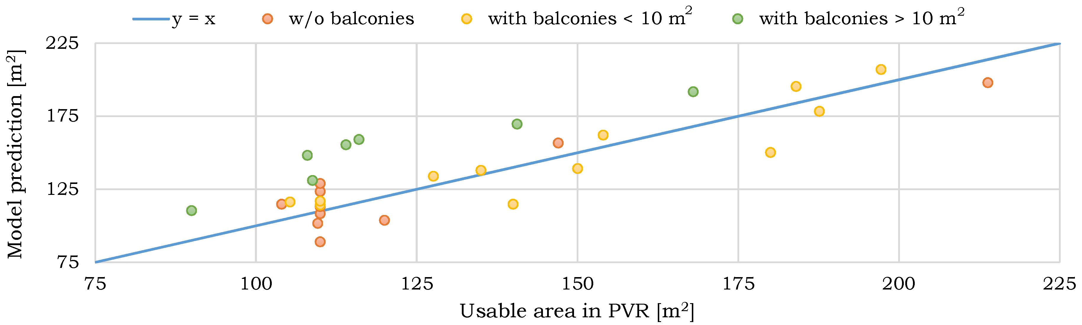
The mean error for the whole dataset amounted to 13.05%. The errors’ median was 10.44%, and maximum and minimum errors were equal to 37.31% and 1.47%, respectively. The model’s inference resulted in the coefficient of determination, $R^2=68.75$%. This significant decrease in accuracy is caused by a number of reasons. First of all, none of the 96 buildings from the design offices, on which the NN was trained, has a balcony within the covered area, and not on the top of the extension at the same time. Simultaneously, out of 29 Koszalin buildings, only 10 have no balcony meeting the criteria stated above. Out of 19 houses that have such balconies, seven is characterized by large balconies’ areas, reaching even 30 m${}^2$. The usable area of each of these buildings was strongly overestimated by the NN.

Removal of these seven buildings resulted in much better predictions’ statistics. The mean error reached 8.6%, the errors’ median—6.86%, while the maximum and minimum errors amounted to 18.97% and 1.47%, respectively, with $R^2$ equal to 84.23%. Such errors were expected for a few reasons. First of all, we do not know the standard according to which usable areas contained in PVR were calculated. NN was trained on PN-ISO 9836:1997 standard, and gave predictions following it. Secondly, owners reporting the usable area to PVR could have done it as for tax purposes. For those, a calculation is done in a very different way. Last but not least, the analyzed buildings from the Rokosowo precinct belong to the old architecture, being built at least 30 years ago. NN was trained on the design offices’ data, which may follow a more modern architectural approach. Nonetheless, the test of the NN on Koszalin buildings proved to be useful: firstly, it indicated its weakness regarding balconies; secondly, the NN accuracy still turned out to be acceptable.

4. Discussion

In this work, we focused on residential single-family buildings with flat roofs. Light Detection and Ranging data in Koszalin exhibit the first level of detail, in which buildings are represented as blocks. To properly estimate the usable areas of houses with more complicated roofs, a higher level of detail data is needed.

Within this study, we prepared two datasets of flat-roof single-family houses. The first was built out of data on buildings from the design offices’ projects available online, and contains 96 examples. The second one consists of data on 29 houses located within the Rokosowo precinct in Koszalin, Poland, provided by the Database of Topographic Objects, Light Detection and Ranging, Price and Value Register, and Google Street View.

On the dataset gathered from the design offices, we trained and tested different models to predict usable areas of houses based on their three-dimensional models. Firstly, we analyzed the performance of the mathematical formula based on architectural assumptions. It exhibited a high accuracy with the mean error of 6.10%, errors’ median of 4.41%, and $R^2$ = 95.37%; however, at the same time, it required a highly detailed information on the building. To minimize the amount of needed data, we moved to machine learning methods, and we found that the model as simple as linear regression can estimate with great accuracy the usable area of one-story buildings without garages and extensions, having as an input only the covered area of the building. The mean error of its predictions was as low as 2.96%. To correctly account for more than one story, garage, and extensions, a neural network model was needed with two hidden layers of 64 and 8 units, respectively. Its mean error amounted to 3.37%, with $R^2$ as high as 97.74%. Finally, we tested this neural network, trained on the first dataset, on 29 Koszalin houses. The mean error was below 9% with $R^2$ equal to 84.23%. Its performance then can be evaluated as satisfying, especially taking into account the fact that we cannot fully trust data contained in the Price and Value Register and recorded usable areas are both calculated in an unknown standard and for an unknown purpose.

While assessing the results as significantly accurate and very promising in terms of possible applications, we acknowledge weaknesses of the designed and trained model. First of all, none of the buildings on which the model was trained has a balcony within the covered area. Within the Koszalin buildings, the largest balconies have areas of the order of 30 m${}^2$, and this is the error that the model has to make. Secondly, none of the methods estimating the building’s usable area based on its three-dimensional model is able to guess architectural solutions that significantly impact the usable area, but are invisible from the outside, like entresols. There is also a possibility that training data, namely the design offices’ model buildings do not exhibit the same diversity of architectural solutions that exist in the reality. Nonetheless, they offer a concise source of data with a minimized human error, and calculated in a known standard. Lastly, the model suffers from the accuracy decrease if the building’s height instead of number of stories is provided. Three solutions to this problem are the following: first, to use Google Street View to determine the number of stories. The second is to apply the mathematical formula we designed to estimate number of stories out of the height. Finally, one can provide the height as a feature, and use the model with slightly worse accuracy. It is also important to note that, even if the presented model was significantly improved and provided excellent results, the legalization and its implementation in Polish Price and Value Register may prove very challenging.

The possible extension of this work is to apply neural networks (or other machine learning model) to estimate usable areas from topographic data of houses with more complex roofs, like gable or hip ones. To achieve this, at least topographic data of second level of detail is needed. It enables recognizing the roof structure as well as secondary construction elements. Moreover, the third level of detail data should account for balconies, and therefore present a full picture needed to calculate the usable area. While the topographic data of a second level of detail are available in the eastern part of Poland, the third level is still not attainable for general public. Such detailed three-dimensional models of houses could be then processed by a chosen model, e.g., convolutional neural networks, which would provide an estimation for the usable area.

5. Conclusions

It is the first, known to the authors, machine learning approach to the usable area estimation based on the buildings’ three-dimensional models. Low mean errors and high determination coefficients of the neural network’s predictions indicate that this merge can prove very fruitful for real estate appraisers. Moreover, the predictions of neural networks will be enhanced, while using the newest standard PN-ISO 9836:1997 with two additional rules introduced by the regulation in 2012 which also made its use mandatory. According to its rules, the partition walls should be ignored in the usable area calculation. With the removal of the error caused by the variance of partition wall density between houses, the neural network could predict the building’s usable area based on three-dimensional model data with an even higher accuracy.

References

- Dawid, L. Characteristics of the Residential Real Estate Market and Their Valuations in 2010–2015 on the Example of Mielno Commune. Appl. Sci. Rev. 2017, 14, 56–71. (In Polish) [Google Scholar]
- Dawid, L. Analysis of Completeness of Data from the Price and Value Register on the Example of Kołobrzeg and Koszalin Districts in Years 2010–2017. Stud. Res. FEM SU 2018, 1, 91–102. (In Polish) [Google Scholar]
- Dawid, L. Analysis of Data Completeness in the Register of Real Estate Prices and Values Used for Real Estate Evaluation on the Example of Koszalin District in the Years 2010–2016. Folia Econ. Stetin. 2018, 18, 17–26. [Google Scholar] [CrossRef]
- The Ordinance of 10 June 2016 on the Promulgation of the Consolidated Text of the Ordinance of the Minister of Regional Development and Construction, Warsaw. Journal of Laws of 2016, Item 1034. Available online: http://prawo.sejm.gov.pl/isap.nsf/DocDetails.xsp?id=WDU20160001034 (accessed on 5 July 2019). (In Polish)
- Bydłosz, J.; Cichociński, P.; Piotr, P. Possibilities of the Register of Real Estates Prices and Values Restrictions Overcoming Applying GIS Tools. Stud. Inform. 2010, 31, 229–244. (In Polish) [Google Scholar]
- Budzyński, T. Calculating the Area of Newly-Built Apartments and Buildings According to Uniform Rules. Geod. R. 2012, 84, 31. (In Polish) [Google Scholar]
- Hopfer, A. The Real Estate Price and Value Register in the Light of the Project of the Regulation of the Council of Ministers on Integrated Information System on Real Estate—Impact of the Mentioned Regulation on Quality and Reliability of PVR. Real Estate Apprais. 2012, 74, 4–11. (In Polish) [Google Scholar]
- Williamson, I. Land Administration for Sustainable Development; ESRI Press Academic: Beijing, China, 2010. [Google Scholar]
- Enemark, S. Building Modern Land Markets in Developed Economies. J. Spat. Sci. 2005, 50, 51–68. [Google Scholar] [CrossRef]
- Enemark, S. From Cadastre to Land Governance: The Role of Land Professionals and FIG. 2010. Available online: https://www.semanticscholar.org/paper/From-Cadastre-to-Land-Governance%3A-The-role-of-land-Enemark/227a1e96079aeccd6ee59be4f84fbd7e2ec5372c (accessed on 1 July 2019).
- Felcenloben, D. Real Estate Cadastre; Gall: Katowice, Poland, 2009; pp. 29–42. (In Polish) [Google Scholar]
- Hycner, R. Basics of the Cadastre; AGH University of Science and Technology Press: Lesser Poland, Poland, 2004; pp. 241–282. (In Polish) [Google Scholar]
- Henssen, J. Basic Principles of the Main Cadastral Systems in the World. In Proceedings of the One Day Seminar held during the Annual Meeting of Commission 7, Cadastre and Rural Land Management, of the International Federation of Surveyors (FIG), Delft, The Netherlands, 16 May 1995. [Google Scholar]
- Bennett, R. On the Nature and Utility of Natural Boundaries for Land and Marine Administration. Land Use Policy 2010, 27, 772–779. [Google Scholar] [CrossRef]
- Bennett, R. Cadastral Futures: Building a New Vision for the Nature and Role of Cadastres. FIG Congr. 2010, 1–11. Available online: https://www.fig.net/resources/monthly_articles/2011/june_2011/june_2011_bennett_rajabifard_et_al.pdf (accessed on 1 July 2019).
- Larsson, G. Land Registration and Cadastral Systems; Longman Scientific and Technical: Harlow, UK, 1991; pp. 21–65. [Google Scholar]
- Kaufmann, J. Cadastre 2014: A Vision for a Future Cadastral System; International Federation of Surveyors: Copenhagen, Denmark, 1998; pp. 1–38. [Google Scholar]
- Stoter, J. Towards a 3D Cadastre: Where Do Cadastral Needs and Technical Possibilities Meet? Comput. Environ. Urban Syst. 2003, 27, 395–410. [Google Scholar] [CrossRef]
- Konowalczuk, J. The Corporate Real Estate Market in Public Statistics in Poland. Real Estate Manag. Valuat. 2014, 22, 41–51. [Google Scholar] [CrossRef] [Green Version]
- Foryś, I.; Kokot, S. Problems with Real Estate Market Analysis. In Microeconomy in Theory and Practice; Res. Bull. Univ. Szczec.: Szczecin, Poland, 2001; pp. 175–182. (In Polish) [Google Scholar]
- Kokot, S. Data Quality of Transaction Prices in Real Estate Market. Acta Sci. Adm. Locorum 2015, 14, 43–49. (In Polish) [Google Scholar]
- Benduch, P.; Hanus, P. The Concept of Estimating Usable Floor Area of Buildings Based on Cadastral Data. Rep. Geod. Geoinform. 2018, 105, 29–41. [Google Scholar] [CrossRef]
- Benduch, P. Legal and Standard Principles of Buildings and Their Parts Usable Floor Area Quantity Surveying. Infrastruct. Ecol. Rural Areas 2018, 1, 225–238. (In Polish) [Google Scholar]
- Act of January 12, 1991 on Local Taxes and Charges. Journal of Laws of 1991, Item 31. Available online: http://prawo.sejm.gov.pl/isap.nsf/DocDetails.xsp?id=WDU19910090031 (accessed on 25 June 2019). (In Polish)
- Act of July 28, 1983 on Tax on Inheritance and Donations. Journal of Laws of 1983, Item 207. Available online: http://prawo.sejm.gov.pl/isap.nsf/DocDetails.xsp?id=WDU19830450207 (accessed on 25 June 2019). (In Polish)
- Act of June 21, 2001 on Tenants Rights, Municipal Housing Stock and the Civil Code Amendment. Journal of Laws of 2001, Item 733. Available online: http://prawo.sejm.gov.pl/isap.nsf/DocDetails.xsp?id=WDU20010710733 (accessed on 25 June 2019). (In Polish)
- Regulation of the Minister of Justice of February 15, 2016 on the Establishment and Maintenance of Land and Mortgage Registers in an IT System. Journal of Laws of 2016, Item 312. Available online: http://prawo.sejm.gov.pl/isap.nsf/DocDetails.xsp?id=WDU20160000312 (accessed on 25 June 2019). (In Polish)
- Normalization Act of April 3, 1993. Journal of Laws of 1993, Item 251. Available online: http://prawo.sejm.gov.pl/isap.nsf/DocDetails.xsp?id=WDU19930550251 (accessed on 26 June 2019). (In Polish)
- Normalization Act of September 12, 2002. Journal of Laws of 2002, Item 1386. Available online: http://prawo.sejm.gov.pl/isap.nsf/DocDetails.xsp?id=WDU20021691386 (accessed on 26 June 2019). (In Polish)
- Polish Commitee of Standardization. PN-70/B-02365 Surface Area of Buildings—Classification, Definitions, and Methods of Measurement 1970. Available online: http://rzeczoznawca-zachodniopomorskie.pl/pliki/PN_70_B_02365.pdf (accessed on 26 June 2019). (In Polish).
- Zbroś, D. The Rules for Calculating the Usable Area by Two Current Polish Standards. Saf. Eng. Anthropog. Objects 2016, 3, 19–22. (In Polish) [Google Scholar]
- Polish Commitee of Standardization. PN-ISO 9836:1997 Performance Standards in Building—Definition and Calculation of Area and Space Indicators 1997. Available online: http://rzeczoznawca-zachodniopomorskie.pl/pliki/PN_ISO_9836_1997.pdf (accessed on 26 June 2019). (In Polish).
- International Organization for Standardization. ISO-9836:1992 Performance Standards in Building—Definition and Calculation of Area and Space Indicators 1992. Available online: https://www.sis.se/api/document/preview/608742/ (accessed on 22 June 2019).
- Regulation of the Minister of Transport, Construction and Maritime Economy of April 25, 2012 on Detailed Scope and Form of a Construction Project. Journal of Laws of 2012, Item 462. Available online: http://prawo.sejm.gov.pl/isap.nsf/DocDetails.xsp?id=WDU20120000462 (accessed on 25 June 2019). (In Polish)
- Polish Commitee of Standardization. PN-ISO 9836:2015-12 Performance Standards in Building—Definition and Calculation of Area and Space Indicators 2015. Available online: http://sklep.pkn.pl/pn-iso-9836-2015-12p.html (accessed on 5 July 2019). (In Polish).
- Garcia-Gutierrez, J.; Martínez-Álvarez, F.; Troncoso, A.; Riquelme, J.C. A Comparative Study of Machine Learning Regression Methods on LiDAR Data: A Case Study; Herrero, Á., Baruque, B., Klett, F., Abraham, A., Snášel, V., de Carvalho, A.C., Bringas, P.G., Zelinka, I., Quintián, H., Corchado, E., Eds.; International Joint Conference SOCO’13-CISIS’13-ICEUTE’13; Springer International Publishing: Cham, Switzerland, 2014; pp. 249–258. [Google Scholar]
- Nahhas, F.H.; Shafri, H.Z.M.; Sameen, M.I.; Pradhan, B.; Mansor, S. Deep Learning Approach for Building Detection Using LiDAR–Orthophoto Fusion. J. Sens. 2018, 2018. [Google Scholar] [CrossRef]
- Verschoof-van der Vaart, W.; Lambers, K. Learning to Look at LiDAR: The Use of R-CNN in the Automated Detection of Archaeological Objects in LiDAR Data from the Netherlands. J. Comput. Appl. Archaeol. 2019, 2, 31–40. [Google Scholar] [CrossRef] [Green Version]
- Marrs, J.; Ni-Meister, W. Machine Learning Techniques for Tree Species Classification Using Co-Registered LiDAR and Hyperspectral Data. Remote Sens. 2019, 11, 819. [Google Scholar] [CrossRef]
- Lipińscy, M.L. Design Office. Houses Projects. Available online: https://lipinscy.pl/ (accessed on 10 July 2019).
- Mendel, B. ARCHON+ Project Office. Available online: https://www.archon.pl/(accessed on 10 July 2019).
- Head Office of Land Surveying and Cartography. Geoportal of National Spatial Data Infrastructure. Available online: https://www.geoportal.gov.pl/ (accessed on 20 July 2019).
- QGIS Development Team. QGIS Geographic Information System. Open Source Geospatial Foundation Project. Available online: http://qgis.osgeo.org. (accessed on 21 July 2019).
- Chrobak, T.; Łabaj, A.; Bolibok, A. (Eds.) Textbook for Participants of Trainings on Possibilities, Forms, and Methods of Using the Database of Topographic Objects; Head Office of Land Surveying and Cartography: Cracow, Poland, 2015. (In Polish) [Google Scholar]
- Rubinowicz, P. Generation of CityGML LoD1 City Models Using BDOT10k and LiDAR Data. Space Form 2017, 31, 61–74. [Google Scholar]
- Wężyk, P. (Ed.) Textbook for Participants of Trainings on Using LiDAR Products; Head Office of Land Surveying and Cartography: Cracow, Poland, 2015. (In Polish) [Google Scholar]
- Schabowicz, K.; Gorzelańczyk, T. General Architecture. Basics of Designing and Calculating Buildings Construction; Lower Silesian Educational Publishing House: Wrocław, Poland, 2017; pp. 50–199. (In Polish) [Google Scholar]
- Michalak, H.; Pyrak, S. Single-Family Houses. Construction and Calculation; ARKADY: Warsaw, Poland, 2006; pp. 164–307. (In Polish) [Google Scholar]
- Piotrowski, R.; Dominiak, P. Construction of a Passive House, Step by Step; Construction Guide: Warsaw, Poland, 2008; pp. 135–198. (In Polish) [Google Scholar]
- Korzeniewski, W. Single-Family Buildings. Usage Requirements and Technical Conditions; Central Office on Construction Information: Warsaw, Poland, 1998; pp. 152–191. (In Polish) [Google Scholar]
- Buczkowski, W. (Ed.) General Architecture, Buildings Construction; ARKADY: Warsaw, Poland, 2009; Volume 4, pp. 7–98. (In Polish)
- Gołuch, A. Architectural-Construction Design; KANON: Gdańsk, Poland, 1998; pp. 241–252. (In Polish) [Google Scholar]
- Draper, N.R.; Smith, H. Applied Regression Analysis, 3rd ed.; Wiley Series in Probability and Statistics; Wiley: Hoboken, NJ, USA, 1998; p. 33. [Google Scholar]
- Aggarwal, C.C. Neural Networks and Deep Learning. A Textbook; Springer: Berlin, Germany, 2018; pp. 4–20. [Google Scholar]
- Singh, A.; Thakur, N.; Sharma, A. A review of supervised machine learning algorithms. In Proceedings of the 3rd INDIACom, New Delhi, India, 16–18 March 2016; pp. 1310–1315. [Google Scholar]
- Kotsiantis, S.B.; Zaharakis, I.D.; Pintelas, P.E. Machine Learning: A Review of Classification and Combining Techniques. Artif. Intell. Rev. 2006, 26, 159. [Google Scholar] [CrossRef]
- Hutter, F.; Hoos, H.; Leyton-Brown, K. An Efficient Approach for Assessing Hyperparameter Importance. In Proceedings of the 31st International Conference on Machine Learning, Beijing, China, 21–26 June 2014; Volume 32, pp. 754–762. [Google Scholar]
- Huber, P.J. Robust Estimation of a Location Parameter. Ann. Stat. 1964, 53. [Google Scholar] [CrossRef]
- Kennedy, P. A Guide to Econometrics; The MIT Press: Cambridge, MA, USA, 2003; pp. 205–206. [Google Scholar]
- Ng, A.; Katanforoosh, K.; Mourri, Y.B. Addressing Data Mismatch. Structuring Machine Learning Projects. 2019. Available online: https://www.coursera.org/lecture/machine-learning-projects/addressing-data-mismatch-biLiy (accessed on 15 August 2019).
- Hołub, A. PN-ISO 9836:2015-12—Further Confusion and Uncertainty. 2016. Available online: https://resources.geodetic.co/norma-pn-iso-98362015-12-kolejne-zamieszanie-i-niepewnosc/ (accessed on 15 August 2019). (In Polish).
- Polish Association of Development Companies. Are Differences in a Flat’s Usable Area Acceptable? Available online: http://pzfd.pl/pzfd-dla-kupujacego/pytania/ (accessed on 1 September 2019). (In Polish).
- The Ordinance of the Council of Ministers of September 21, 2004 on Real Estate Valuation and Preparation of Valuation Survey. Journal Laws of 2004, Item 2109. Available online: http://prawo.sejm.gov.pl/isap.nsf/DocDetails.xsp?id=WDU20042072109 (accessed on 20 June 2019). (In Polish)
Figure 1.
The results of the formula estimation with distinction between buildings with and without garages. The coefficients of determination are as following: without garages = 98.28%, with garages = 94.77%, total = 95.37%
Figure 2.
Predictions of (a) the linear regression () and (b) neural network with eight hidden units () with distinction between one- and two-story buildings. Input features: the covered area, and the number of stories, .
Figure 3.
Predictions of the NN (4-64-8-1), for 29 Koszalin flat-roof single-family buildings with distinction between buildings with and without balconies. Input features: the covered area, , number of stories, , number of garage spots, , and percentage of extension area in , .