Infrared Optical Observability of an Earth Entry Orbital Test Vehicle Using Ground-Based Remote Sensors


1
Key Laboratory of Aerospace Thermophysics of Ministry of Industry and Information Technology, Harbin Institute of Technology, 92 West Dazhi Street, Harbin 150001, China
2
School of Energy Science and Engineering, Harbin Institute of Technology, 92 West Dazhi Street, Harbin 150001, China
*
Author to whom correspondence should be addressed.
Remote Sens. 2019, 11(20), 2404; https://doi.org/10.3390/rs11202404
Submission received: 9 September 2019
/
Revised: 12 October 2019
/
Accepted: 13 October 2019
/
Published: 16 October 2019
(This article belongs to the Special Issue Remote Sensing for Target Object Detection and Identification)
Abstract
:Optical design parameters for a ground-based infrared sensor rely strongly on the target’s optical radiation properties. Infrared (IR) optical observability and imaging simulations of an Earth entry vehicle were evaluated using a comprehensive numerical model. Based on a ground-based IR detection system, this model considered many physical mechanisms including thermochemical nonequilibrium reacting flow, radiative properties, optical propagation, detection range, atmospheric transmittance, and imaging processes. An orbital test vehicle (OTV) was selected as the research object for analysis of its observability using a ground-based infrared system. IR radiance contours, maximum detecting range (MDR), and thermal infrared (TIR) pixel arrangement were modeled. The results show that the distribution of IR radiance is strongly dependent on the angle of observation and the spectral band. Several special phenomena, including a strong receiving region (SRR), a characteristic attitude, a blind zone, and an equivalent zone, are all found in the varying altitude MDR distributions of mid-wavelength infrared (MWIR) and long-wavelength infrared (LWIR) irradiances. In addition, the possible increase in detectivity can greatly improve the MDR at high altitudes, especially for the backward and forward views. The difference in the peak radiance of the LWIR images is within one order of magnitude, but the difference in that of the MWIR images varies greatly. Analyses and results indicate that this model can provide guidance in the design of remote ground-based detection systems.
1. Introduction
The use of ground-based remote sensing detectors is becoming an important method of accessing information on trajectories, positions, and flight conditions in the growing field of space technology. Recently, a very promising type of orbital test vehicle (OTV) came to the attention of many space agencies [1]. It is believed to be a candidate for the next generation of space planes and can be reused repeatedly due to low launch costs and high-speed maneuverability. A typical representative of this type of OTV is the X-37B spaceplane [2]. The aircraft can maintain operations in space for several months at a time, like a satellite, and can then return to the Earth’s atmosphere on its own. During the entry phase, it is essential to track the vehicle’s trajectory and flight behavior. Up to now, thermal infrared (TIR) remote sensing technology is widely used for monitoring the background environment and aerial targets [3,4]. However, numerical studies of this technique are rare due to the attendant complexity of the physical processes.
The study of the observability of aircraft based on the TIR effect is a thermal–optical problem. During the entry phase, the air around the aircraft undergoes strong compression along with high frictional forces acting on the aircraft body, resulting in hot reaction air flows. In the high-temperature flow field, many chemical reactions occur including dissociation, ionization, and recombination [5,6]. Under these conditions, air components, consisting of atoms, ions, and molecules, radiate strong optical radiation [7]. For the gas molecules, the process of vibrational transition produces infrared radiation. In addition, the aero-heating effect is also serious and causes a rapid increase in the temperature of the aircraft’s surface, from which strong radiation can also be emitted. Infrared radiation from gases (including air dissociation products and trace air components) in the flow field and the surface is partially absorbed by the surrounding gases in the transmission process. The absorption process has strong spectral band selectivity and can be divided into two regions: (a) self-radiation emitted from the surface and hot gases in the high-temperature region, and (b) the atmospheric transmission effect in the low-temperature region. The infrared radiation of the target and the radiation noise of the environmental background are received by the optical sensor using Earth’s atmospheric attenuation. The radiation is converted into electrical signals and then recognized by the infrared (IR) detector.
Lots of investigations on target detection were conducted for analysis of the aircraft IR signature. Mahulikar et al. [8,9,10] took a low-altitude fighter as a research object to analyze the role of atmosphere in IR signature, and the relationship between IR signature level and target susceptibility. Pan et al. [11] predicted the IR radiation and stealth characteristics for the cabin of a supersonic aircraft. Huang and Ji [12] investigated the effect of environmental radiation on the long-wave IR signature of a cruise aircraft. In these studies, they focused mainly on the surface emission and the exhaust plume under a low-temperature low-altitude condition. However, a comprehensive model that can be used for analysis of the observability of hypersonic vehicles considering the high-temperature gas effect is still rarely reported.
In the context of multi-mode detection requirements, ground-based remote detection saw much development [13,14,15]. Some relevant observations of hypersonic aircraft were conducted with the aid of TIR emissions. These experiments focused mainly on two aspects: TIR imaging of the space transportation system (STS) and radiative heating of sample return capsules (SRC). For instance, NASA carried out a series of hypersonic thermodynamic IR measurements (HYTHIRM) that relied on aerial and ground-based infrared imaging systems [15,16]. The infrared images were used to determine the surface temperature distribution on the viewable windward surface of the shuttle orbiter. These observations of the SRC reentering the Earth’s atmosphere [17,18,19] were mainly concerned with the near-infrared band, with the aim of verifying the radiation excitation mechanisms and flow structures. However, those observations did not provide evaluation models and did not report on the maximum detection range (MDR).
The MDR is an important parameter in the design of optical instruments, which reflects the performance of the detection system. In most cases, it is appropriate that the target is treated as a point source when the aircraft’s irradiance image only fills one or a few pixels of the sensor [20]. Prior literature [13,20,21] indicated that the MDR of an infrared imaging system is a function of factors such as background environment, target radiation characteristics, atmospheric transmittance, and the system threshold signal-to-noise ratio (SNR). Recently, Zhao et al. [21] proposed a spectral bisection method for calculating the operating distance of IR systems based on the MODTRAN (moderate spectral resolution atmospheric transmittance algorithm and computer model) program. Ren et al. [22] suggested a new formula for calculating the atmospheric transmittance based on the LOWTRAN (low-resolution atmospheric transmission) database. Huang et al. [20] reported a photoelectric detection method based on a long-wavelength infrared (LWIR, 8–14 μm) fisheye imaging system. In these literature sources, the target was specified as a uniform low-temperature gray body without gas emissions. However, such a treatment is overly simplistic. In fact, the surface temperature of a hypersonic vehicle may reach 2000 K with a non-uniform distribution [23]. The TIR emission can also be radiated from gases in the shock layer and wake flows [24]. This means that the temperature of both the aircraft’s surfaces and the reacting flows may influence the evaluation of infrared optical observability.
Up to now, it remains a challenge to establish models to investigate the detectability and imaging of a hypersonic vehicle based on its detailed radiative properties. To obtain the irradiance received by a detector, lots of parameters should be calculated such as reacting flows, surface temperature, species concentrations, absorption coefficients, reconstructed nodes, and optical path. These require knowledge of fluid mechanics, spectroscopy, thermochemistry, and optics.
In this study, a comprehensive physical model was proposed to simulate the MDR and the TIR image of an Earth entry OTV. Firstly, the hot reacting flows and surface temperatures were simulated using a thermochemical gas-solid interaction computational fluid dynamics (CFD) solver. In addition, the optical radiative properties of radiating species were evaluated in thermal equilibrium and nonequilibrium. Then, TIR radiance characteristics were computed by solving the radiative transfer equation (RTE) in a fluid inclusion. Furthermore, using the concept of the point source, the MDR was simulated in different bands, trajectory points, and observation angles. Finally, the effects of sensor detectivity on the MDR and the TIR images in the aperture of the detector were discussed and analyzed.
2. Description of Physical Processes in Ground-Based Observation
An Earth entry OTV, with similar geometry to the X-37B [2], was used in this study. After entering the atmosphere, the aircraft flies in a typical flight path, and its velocity as function of altitude for the X-37B was reported in Reference [25], as shown in the lower right of Figure 1. During the entry phase, the air around the aircraft is heated to an extremely high temperature. Under this condition, there are two strong TIR radiation sources: (1) hot air components and gaseous products from dissociation, ionization, and recombination chemical reactions, and (2) glowing aircraft surfaces. These TIR radiations can be received by an IR detection system after being attenuated by passing the Earth’s atmosphere.
For the air around the OTV, the flows are hypersonic and go through chemical nonequilibrium and thermal nonequilibrium conditions due to the drastic environmental changes. Figure 1 shows three typical thermal–chemical regions [26]. For the vehicle surface, the wall temperature depends on the aero-heating, structure heat conduction, radiation, etc. Due to the presence of atmospheric windows as illustrated in the lower left of Figure 1, the spectral bands of interest are generally medium-wavelength infrared (MWIR), with a wavelength of 3–5 μm, and LWIR [27]. At a flight altitude H above sea level (ASL), the ground-based infrared system A can receive the TIR radiation from aircraft B or B1.
During the observation process, changes in the aspect angle between the detector and the aircraft may exert an arbitrary effect on observability. Considering the Earth’s radius Rearth = 6371 km, there is an MDR above the horizon Rmax, as shown in Figure 1. Below this MDR, the TIR intensity and distribution of the target can be imaged in the aperture of the infrared system. This study focuses mainly on the MDR and the TIR imaging during OTV entry.
3. Computational Methods
3.1. Description of CFD Solver
For hypersonic flows above 40 km, the time scale of the chemical and the internal energy exchange processes is comparable with the characteristic time of flows [5]. The internal energy exchange should be described through multiple temperatures. Recently, our research group carried out a series of simulations of hypersonic reacting flows using an in-house code [5,6]. In the code, a two-temperature CFD solver is available for predictions of thermal–chemical nonequilibrium flows. On assuming continuous flows are valid, three-dimensional Reynolds-averaged Navier–Stokes (N–S) equations are solved with a structured implicit scheme with the finite volume method (FVM). The viscous and inviscid fluxes are computed using a central difference and Roe’s averaging scheme [28], respectively. Yee’s symmetric total variation diminishing (STVD) limiter [29] is employed for accurate predictions of the shock layer. The two-equation shear stress transport (SST) with compressible correction is used for the flow simulations in the supersonic–hypersonic regime.
3.2. Optical Radiation and Transfer Models
3.2.1. Optical Radiative Properties of High-Temperature Gases
Studies [30,31] demonstrated that gaseous molecules of NO, CO2, and H2O are the main radiating components of air. Among these species, CO2 and H2O belong to the set of trace components and have a low number density. For instance, the volume fraction of CO2 at ground level is approximately 3.628 × 10⁻⁴, which is two orders of magnitude lower than that of H2O. In hypersonic flows, their number densities are associated with the degree of compression of the flow field. For NO, it is the product of the combination reaction O + N → NO in air, and its formation is related to the dissociation reactions N2 → 2N and O2 → 2O. Generally, high-altitude hypersonic flows are in local thermodynamic nonequilibrium (non-LTE) [32]. In this case, the optical radiation properties of radiating species should be evaluated under non-LTE conditions.
Currently, the new total internal partition sums (TIPS) routine [33] can be used for partition function calculations for some components, including CO2 at temperatures below 5000 K and H2O at temperatures below 6000 K. Based on the known partition function, the spectral lines of the corresponding molecules can be calculated with the aid of the high-temperature database HITEMP [34] (only the spectral lines in the standard conditions are provided). The TIPS routine provides an applicable range for NO at temperatures under 3500 K. The application is limited for high-temperature flows. Thus, a partition function suitable for high temperatures should be used. According to one of the basic principles of quantum mechanics, the reduced partition function of NO can be determined using Equation (1), neglecting the interaction between rotational and vibrational states [34].
where dvib and drot are the degeneracy factors for states, and Gvib and Frot are the term values of vibrational and rotational states, respectively. These parameters can be imported from Reference [35].
Relying on the partition function Q(T), the high-temperature line intensity at a given wavenumber η can be calculated using the correction formula below.
where S(Tref) is the line intensity under standard conditions; h, c, and kB are the Planck constant, the speed of light, and the Boltzmann constant, respectively. El stands for the energy of the lower state. The absorption coefficient of each species within the specified wavenumber and temperature intervals can then be calculated using the line-by-line (LBL) method [36].
where N is the number density of species, and Φ is the line shape function, for which the Voigt line profile [37] is often recommended. Finally, the total absorption coefficient of the mixture can be computed on the assumption that the absorption coefficient is cumulative for each species.
3.2.2. Optical Radiative Properties of High-Temperature Surfaces
For the surface, the radiation intensity is determined using the temperature and emissivity, along with the radiative properties of the surface element calculated in accordance with Planck’s radiation law for a gray body [36].
where C1 and C2 are the first and second radiation constants, respectively; ε is the emissivity, Iλ,sur is the radiance for a thermal source of the surface element, and λ is the wavelength which can be converted to the wavenumber η. The surface emission requires coupling with the gas radiation along the optical path of light propagation.
High-temperature gas radiation differs from the gray-body radiation characteristics of the surface. Its self-emission and self-absorption properties need to be taken into consideration. The total radiation spectral intensity can be calculated using discrete path intervals. Specifically, it can be described using the RTE [36].
where λ indicates the wavelength, and Iλ is the local spectral intensity. Ib,λ is the Planck blackbody function, whereas s and represent the position and the optical path vector, respectively.
Methods commonly used to solve the RTE include the line-of-sight (LOS), ray tracing (RT), and Monte Carlo (MC) methods. Under the condition of an absence of scattering particles, the LOS method is equivalent to the other two. Thus, the LOS method was applied in this study due to a compromise between computational cost and accuracy. The LOS method was introduced in our previous studies [5,38]. LOS starts with a surface element, and the surface emission Iλ,sur can be treated as the initial value of the RTE. According to the RTE, the spectral intensity of the target can be calculated by summing the radiance from each path interval as follows:
where M is the number of segments in optical path, and Iη,tar is the radiance at the wavenumber η in a inclusion with a cutoff value equal to the ambient condition.
3.3. Infrared Optical Observability of Ground-Based Sensors
3.3.1. Detection Range Model
For the optical detection system, the spectrum intensity that arrives at the detector is given by
where R is the distance between the target and the detector, τ(λ,R) is the atmospheric transmittance with a distance of R, At is the effective radiation area of the target surface, τ0(λ) stands for the spectral transmittance of the optical system, A0 is the pupil area of the objective lens system, and Iλ,bg denotes the background radiance received by detector.
The optical radiant power must be converted into a signal voltage, which is integrated within the wavelengths of λl–λu and has the following form [21]:
where D*(λ) is the normalized system detectivity, Δf is the frequency bandwidth of the detector circuitry, Ad is the pixel area of the detector, g is the photoconductive gain, and λu and λl stand for the upper and lower limits of wavelengths for the band of interest.
According to the above equations, the detection distance of the optical system with respect to a point target can be written as
In Equation (9), ΔVs/Vn is the SNR of the system. Based on the noise equivalent flux density (NEFD) [39], which is defined as the incoming TIR power per unit area at the aperture, the sensor parameters (A0, D*, Ad, and Δf) can be integrated into an evaluation parameter. In this study, the background is the deep space. The basic value of the NEFD is 10−12 W/cm2, and the SNR is specified as 5. According to these threshold values, R is the longest detecting range, namely, the MDR.
3.3.2. Atmospheric Transmittance and Radiance
In addition to the main components of nitrogen and oxygen, the atmosphere has a variety of trace components that possess properties of radiation emission and absorption in the corresponding spectral bands. The atmospheric transmittance is a complex parameter due to the selective absorption of atmospheric molecules and the change in atmospheric density with altitude. Therefore, the TIR radiation emitted from the high-temperature fluid inclusion can be absorbed partially by these components, which means that the atmospheric transmittance and self-emission need to be calculated. In the atmospheric environment, the spectral radiation and transmittance of the atmosphere are associated with the path and the spectral band. In this study, the MODTRAN computer program [40] was utilized, which is a moderate-resolution atmospheric radiation transfer model developed by LOWTRAN that can provide atmospheric information for different paths and spectral bands, including atmospheric transmittance, background radiation (e.g., rural, urban, marine, and desert), and solar irradiance in different seasons covering ultraviolent, visible, and infrared wave bands.
In the desired wavelength range of λl–λu, the spectral band is divided into many equally spaced segments Δλ = λi+1 − λi, i = 1, 2, …, n. When the interval Δλ is sufficiently small, the atmospheric transmittance and radiance in the interval wavelength of λi can be expressed as
Based on the abovementioned treatment, the atmospheric transmittance and radiance for the detecting distance R have the following expressions:
Similarly, the atmospheric spectral radiation intensity can be also given as
Based on the self-radiation spectrum and the atmospheric transmittance, the attenuated spectrum can be obtained, and then the radiance can be computed by integrating the attenuated spectrum within the required band.
3.3.3. TIR Smoothing Distribution on the Sensor Aperture
Under detection distances below the MDR, the aircraft surface is partially detected along the detection direction. This means that occlusion occurs in the detecting process. The TIR light rays are emitted from the visible surface through the hot gases and undergo atmospheric attenuation and then arrive at the aperture of the sensor. Usually, the geometric model of an aircraft is complex, and its shell meshes consist of many uniformly arranged grids. However, the pixels of the detector are arranged in an orthogonal array. A common occurrence involves more than one light ray arriving at one pixel. In the pixel, the TIR intensity may be assigned to the center node in the imaging process, which results in an unsmooth TIR image with many bright spots. Therefore, imaging techniques are used to deal with such imaging problems, including the treatment of visible surfaces and mesh clipping.
Visible surface elements that are associated with the LOS direction are required in Equation (7). This is attributed to the fact that the detector only receives the TIR irradiance of partial surfaces. As shown in Figure 2a,b, there are two types of occlusion elements. One is a surface element with radiation directions that have no component in the LOS direction, and the other is a surface element obscured by the other elements. A flag 0 represents the invisible surface elements using the following expression:
where is the outward normal of the target surface element Ai, and Vi,p is the pth vertex of the element Ai. {Aj,j≠i} represents the set of the surface elements excluding Ai, where j =1, 2, …, Nelement.
The imaging process must calculate the irradiance received by each pixel of the detector, as shown in Figure 2c. In this process, part of the surface element projected onto the pixel needs to be retained for evaluation. In order to produce an accurate image, each separate region should be calculated in each individual pixel. As shown in Figure 2d, mesh clipping can be used for computing the area of the polygon V4V1IJKL. This procedure requires the vertices of the two sets (A, B, C, D and V1, V2, V3, V4) and their candidate intersection points (W1, I, J, K, L, W2, W3, W4). The desired points should then be selected from these vertices and intersection points. These unordered points must be arranged before forming a closed polygon. A clockwise arrangement is established according to the cosine value of the vertices as shown in Figure 2e.
In Figure 2f, a representative case is shown, in which the pixel element receives a total of TIR radiation intensity from nine surface elements. According to the above image treatment, the irradiance received by each detector pixel can be calculated by the following formula:
where q is the radiant energy of the pixel, I is the TIR intensity received by the system which is emitted from the surface element k, and Ai,j,k represents the visible area of the kth surface element in the i × j pixel.
3.4. Computational Flow Chart of MDR
A code was programed in FORTRAN considering above physical models. In these procedures, the fluid computation is decoupled with the radiative computation on the assumption that the gas and surface emissions have little influence on the flow field parameters. The computational flow chart is shown in Figure 3. Firstly, the reacting flow and surface temperature can be obtained using a two-temperature CFD solver based on the known freestream conditions and the structured grid [41]. The radiative properties of gases, including CO2, NO, and H2O, are evaluated relying on the HITEMP database. Then, at a specified observation angle, the occlusion effect is considered, and the visible parts of the aircraft are computed. Furthermore, the spectral irradiance is achieved along the LOS direction in a fluid-domain inclusion. An initial detecting distance that is larger than the aircraft’s flight altitude is given and used for the computation of the irradiance received by the sensor. Finally, the MDR can be obtained by comparing with the detectivity of the sensor.
3.5. Validations of Physical Models
At present, to the best of the authors’ knowledge, there are few reports on the radiation observation data of hypersonic vehicles. In most cases, it is difficult to obtain the self-radiation intensity of a hypersonic vehicle due to expensive measurement costs, complex test conditions, and strong background noises. Up to now, calculations of the thermo-chemical nonequilibrium flow field and the high-temperature nonequilibrium radiation characteristics of radiating gases are still challenging tasks. Therefore, the physical models are verified separately against reference data in this paper.
3.5.1. Validations of Surface Temperature and Flow Field Parameters
From the two strong TIR radiation sources, accurately predicting the surface temperature and flow field parameters is important. In this section, two available reference data are used for validation studies of the surface temperature and the flow field parameters: (1) double-cone UHTC (Ultra-high temperature ceramics) surface temperature test in the L2K wind tunnel at DLR (German Aerospace Center) Köln in Germany [42], and (2) reference data of the ELECTRE [43] vehicle at 293 s reported by Hao et al. [44]. The detailed computational parameters were given in our previous work [6,41] including the geometry size, material thermal properties, grids, boundary conditions, and so forth. In Figure 4, comparisons between computed results and reference data prove that the current CFD solver has good performance in predictions of the surface temperature and flow field parameters of the hypersonic vehicle. This work can assist in a study of ground-based IR optical observability and imaging for an Earth entry vehicle.
3.5.2. Validations of High-Temperature Optical Radiative Properties
The dual-mode experiment on bow-shock interactions (DEBI) [45,46] was carried out in 2003. In flight measurements, spectrometers mounted in the nose cone of a sounding rocket were used for measuring the forward- and side-looking radiation signatures in the bow-shock layer. Ozawa et al. [46] computed the forward-looking infrared spectrum at 40 km and 3.5 km/s using nonequilibrium radiation distribution (NERD) and the NEQAIR-IR (nonequilibrium air radiation-infrared) program. These data can be used to verify the current optical radiative property computational model.
The DEBI vehicle has a blunt cone with a 0.2032-m-radius nose and a 7.5° half-cone angle. The computational parameters can be seen in Reference [46]. The flow field parameters were computed using the two-temperature CFD solver, which can be treated as the input data in radiation computations. Based on radiative properties of high-temperature gases using the LBL method, the forward-looking infrared spectrum of the shock layer can be obtained, as shown in Figure 5. A comparison of the infrared spectrum between computed and reference data indicates that the current model is in good agreement with the results of NERD and NEQAIR-IR.
3.5.3. Validations of Infrared Optical Observability
In this paper, the detection range calculation model was derived from the NEFD model, which is based on the relationship between the total target flux density at the sensor location and the SNR, namely, NEFD = Ptar/SNR. The target flux density Ptar was mainly determined by the target’s self-radiation intensity and atmospheric transmission. NEFD was determined by the sensor performance and the background radiated noise. The reliability of the NEFD and SNR models was validated against the observation results of a laboratory temperature-controlled blackbody by Richter and Fries [47]. It is demonstrated that the error between the SNR based on the NEFD model and the experimental measurements is less than 5%. Therefore, the reliability of the infrared optical observability module is determined by the target flux density Ptar, which depends on the radiation transfer calculation model.
An available reference dataset to verify the current transfer model is the ground-based observation of an Atlas rocket exhaust plume. The observation schematic diagram is shown in Figure 6a. In Reference [48], infrared radiation spectra of the Atlas rocket exhaust plume are numerically presented. Detailed calculation conditions (geometry, boundary, inflow, etc.) of the plume were given in Reference [48] and our prior work [49,50]. In this section, self-radiation of the exhaust plume is studied using our IRSAT (infrared signature analysis tool) code [49], whereby the spectrum can be used to compute the apparent radiation received by the sensor using the model described in Section 3.3. The calculation steps are as follows: (1) the self-radiation spectrum of the plume is obtained without soot at the altitude of H = 40 km by IRSAT, and (2) the apparent radiation spectrum is calculated at the pupil of the sensor using the module in Section 3.3, in which the plume is treated as a point source. A comparison of the apparent radiation spectrum received by the sensor between computed and reference results is shown in Figure 6b. It is indicated that results of the current infrared optical observability model are in good agreement with the reference data.
4. Results
4.1. Thermal–Optical Flow Field
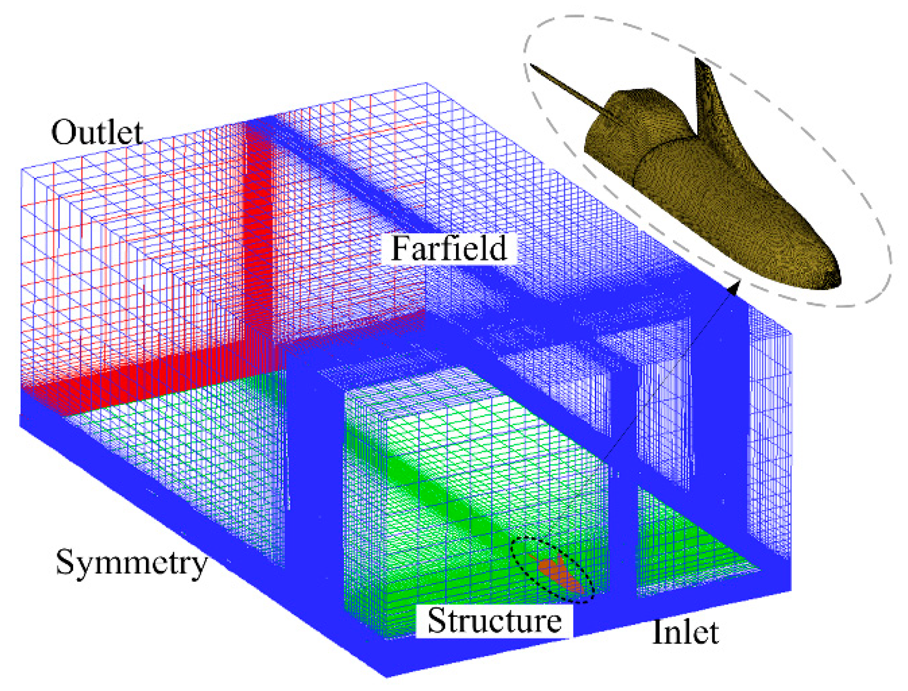
In this study, a cube calculation domain was adopted for the OTV. Considering the symmetry of the geometry, one half of the geometric model was used for fluid simulations. All grids were structured, and their distribution is shown in Figure 7. For the conjunction heat transfer calculation, the computational domain was divided into fluid and structure domains. The grids of the two computational domains demonstrated a one-to-one correspondence at the interface. Generating grids in two domains used a total of 102 blocks. The fluid domain consisted of 23 million grids, and the solid domain contained 1.24 million grids with 80,000 shell grids. It was indicated in previous studies that the mesh Reynolds number should be kept below two to guarantee the precision of the heat flux on the surface of a hypersonic aircraft [51]. Therefore, the first wall–normal spacing from the wall was arranged to be approximately 1 × 10⁻⁵ m from the wall in this study. In addition, grids near the wall and in the potential shock-layer region were also refined.
In the calculations, the inflow and far-field boundaries applied free stream conditions with uniform pressure and temperature. A supersonic outflow boundary was employed. The gas–solid interface was specified for the fluid and structure sides, respectively. The structural materials were assumed to be the stainless steel, whose properties can be seen in Reference [42]. In the structure domain, a radiative transfer wall with an emissivity of 0.85 was specified at the outer surface, and a wall with an initial wall temperature of 300 K was used for the inner surface. According to the OTV’s flight regime as shown in Figure 1, seven computing trajectory points were selected for analytical calculations. In this study, it was assumed that the angle of attack (AOA) was zero during the flight and that the flow field reached the steady state at these computing points. The detailed freestream conditions are listed in Table 1.
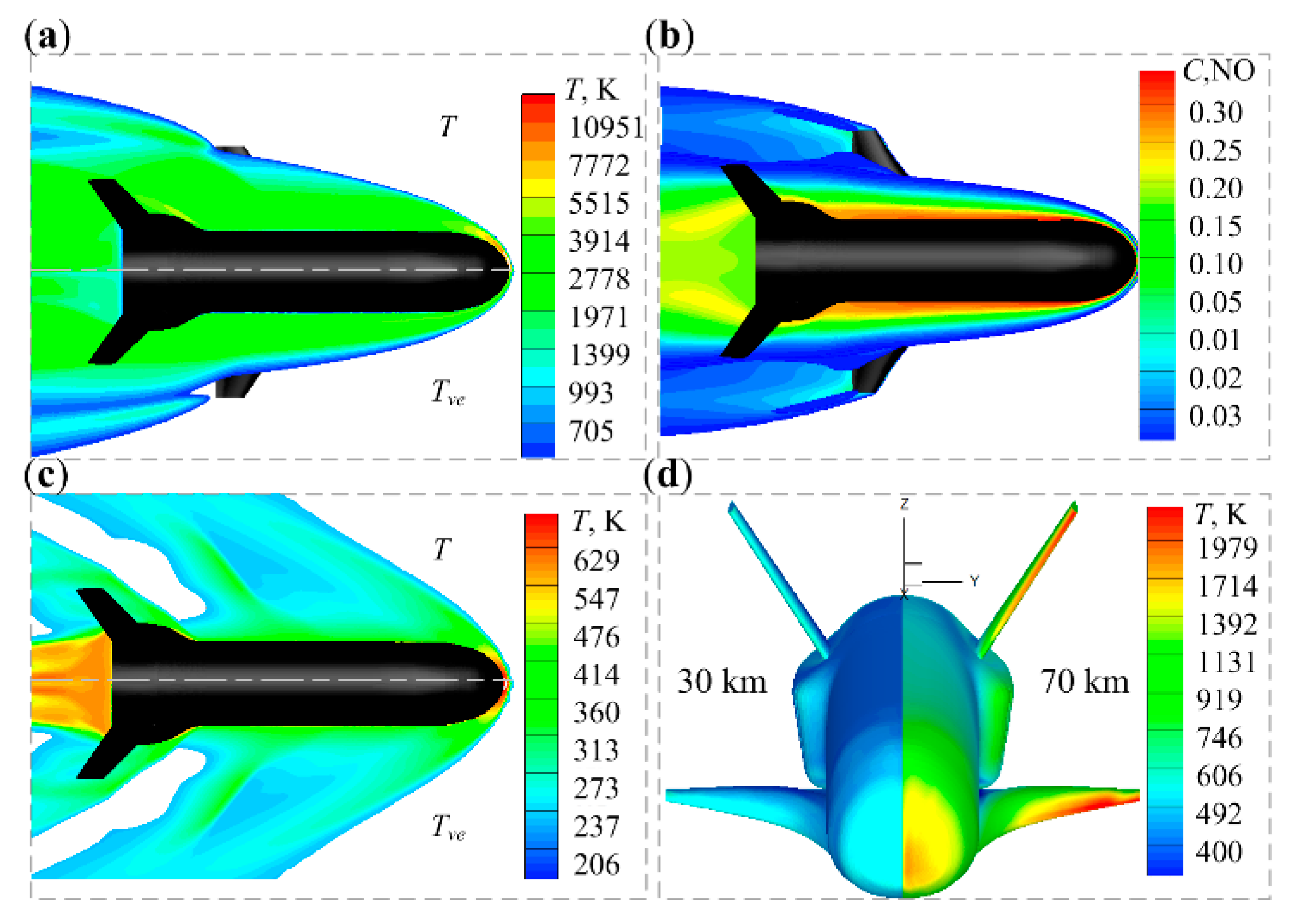
Based on these conditions, the steady reacting flows in these cases were calculated. A machine with 52 central processing unit (CPU) cores was used for parallel computation, taking about 80 h to calculate the flow field for each computational case. The contours of the flow field parameters in the two representative cases (30 km and 70 km) are shown in Figure 8, including the surface temperature, fluid temperature, and species distribution.
4.2. Self-Emission of OTV
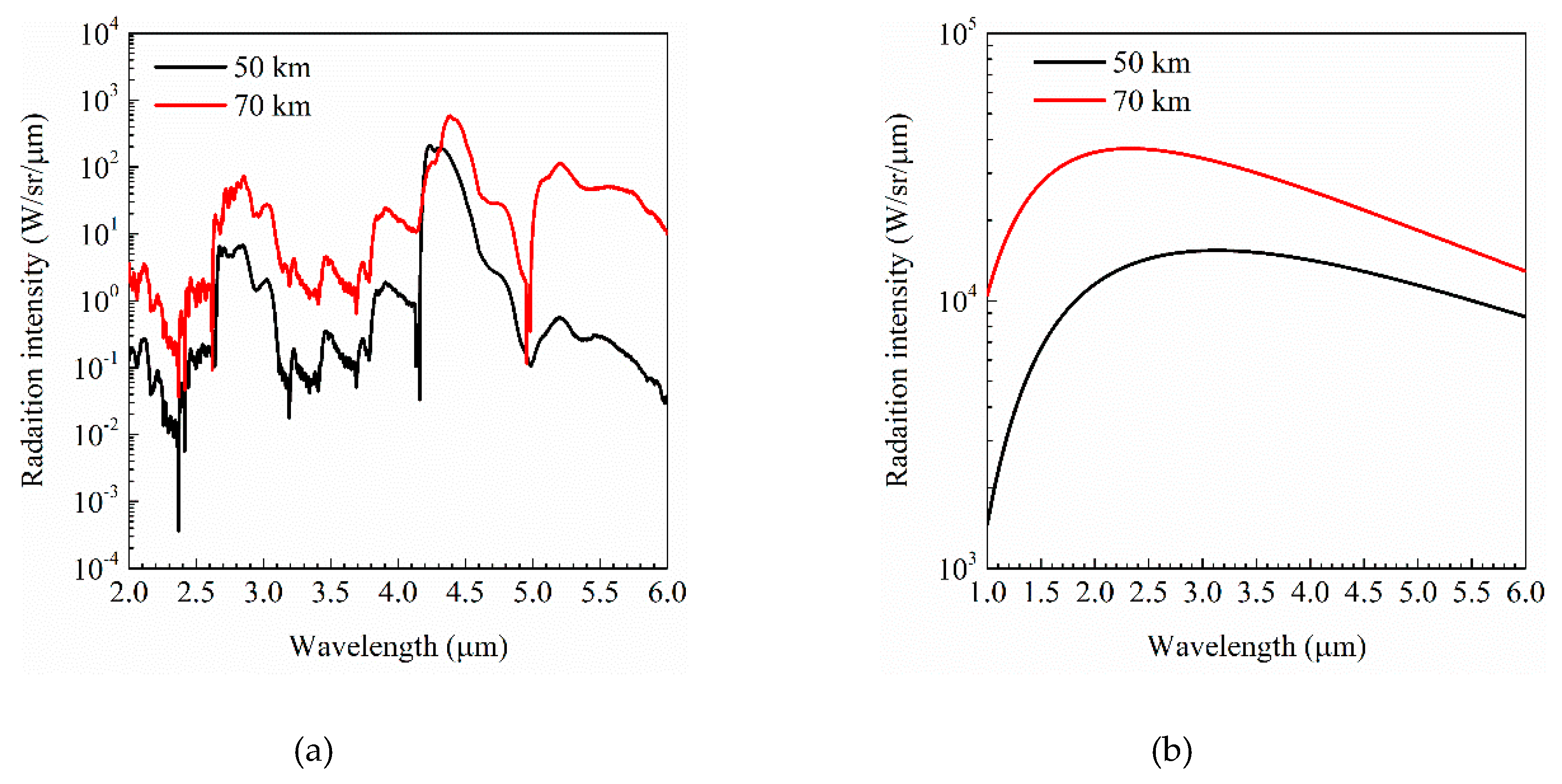
Self-emission is defined as the radiance in the fluid inclusion within an ambient cutoff temperature. It is the radiance of the glowing surface and hot gases occupying a small space before considering atmospheric attenuation. In this study, gas emissions of the four species including NO, CO, CO2, and H2O were considered. Profiles of the radiance of two groups of typical detecting angles, described by θ1 and θ2, are plotted in Figure 9. It can be seen from these illustrations that the distribution of radiation intensity is associated with spectral bands and detecting angles. For different computing points, the radiance distribution within the same band is similar, but the radiation intensity is quite different. In order to examine the contribution of the gas and the surface to the radiance, the spectrum distribution at the angle of θ1 = 0° is shown in Figure 10.
As a matter of fact, the detecting angle may be arbitrary during target detection. An angular coordinate system was used to describe the radiance distribution at all possible angle. The observation angle can be described by a pair of the circumferential angle (φ) and the zenith angle (θ). The x-axis is defined as being in the direction toward the nose of the aircraft, while the z-axis is toward the back of the aircraft. φ is the angle between the direction vector and the x-axis within the range of 0°–360°. θ is the angle between the direction vector and the z-axis within the range of 0°–180°.
Figure 11 shows the contours of the radiance for the two representative cases of 30 km and 70 km in 2π space, which shows that the distribution of radiance is strongly dependent on the angle of observation and the spectral band. The peak intensity distributions for different computing points of the two bands are shown in Figure 12.
4.3. Detecting Distance of the Ground-Based Sensor
Based on the above radiance, the MDR could be evaluated by considering the atmospheric transmittance. In the calculation, a discrete angle of 10° was used for the angles of θ and φ, and a total of 722 observation angles were considered in 2π space. It should be noted that the occlusion of the horizon was also considered in calculating the detecting distance, as shown in Figure 1.
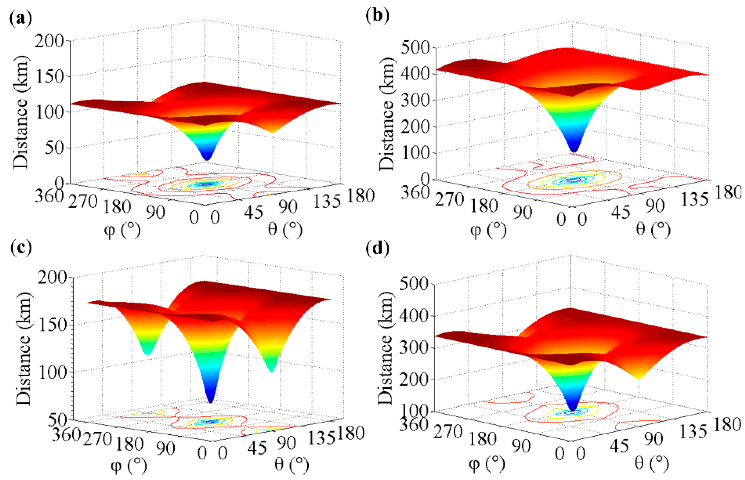
On the assumption that the NEFD was 10−12 W/cm2, the MDR contours within the MWIR and LWIR bands are shown in Figure 13. It can be seen from the figure that the MDR of the rear-most parts of the aircraft (θ = 90°, φ = 180°) was the shortest. This was attributed to the low-temperature tail section and parts concealed by the high-temperature gas in the shock layer and partial surfaces. Figure 13c also presents a three-peak structure, which is distinctly different from the other three illustrations. In the 30-km case, the MDR of the MWIR band was greater than that of the LWIR, which was reversed in the 70-km case. This phenomenon was similar to the distribution of the radiance as shown in Figure 11. The MDR profiles of the MWIR and LWIR bands as a function of the altitude are shown in Figure 14.
4.4. Effect of Sensor Detectivity on MDR
To examine the effect of the detectivity on the MDR, a detectivity equivalent of NEFD = 10−14 W/cm2 is employed in this section. Figure 15 shows the profiles of the peak MDR for seven computing points. The MDR profiles for the MWIR and LWIR bands also intersected at the characteristic altitude of 40 km. Comparing these results with Figure 14 shows that the characteristic altitude decreased as the detectivity increased. Above 40 km, the peak MDR did not drop, as shown in Figure 14.
Figure 16 shows the contours of the MDR increment for different detection angles from NEFD = 10−12 W/cm2 to NEFD = 10−14 W/cm2. Profiles of the peak increment of the MDR are shown in Figure 17. It can be seen from this figure that the peak MDR increment increased as the altitude increased. The increments of the two bands were almost identical at altitudes of 30 km and 70 km. In this region, the maximum increment of the MDR in the MWIR band was higher than that in the LWIR band. This indicates that the increase in detectivity was helpful for increasing performance in the MWIR band.
4.5. Infrared Optical Image of the Sensor
While below the MDR, the aircraft’s optical signature can be received by the pupil aperture of the detection system, and the TIR image fills the detector’s pixels. At greater distances, the TIR intensity is captured by only a few pixels. To examine the distribution of radiant energy in the detector pixels, the imaging characteristics of the OTV are analyzed in this section.
Imaging is associated with the field of view (FOV) and the resolution of the detection system. Usually, the FOV of the scanning telescope has a wide range of 0.01–100 mrad [52,53,54]. As the FOV and the detection distance increase, the number of pixels receiving the TIR irradiance decreases. This number may even decease to one or a few pixels. In this study, three artificial FOVs were used for analyzing the distribution of TIR images, including α/2 = 0.01°, α/2 = 0.05°, and α/2 = 0.1°. All calculations were simulated on the assumption that the aperture of the system consisted of 100 × 100 pixels.
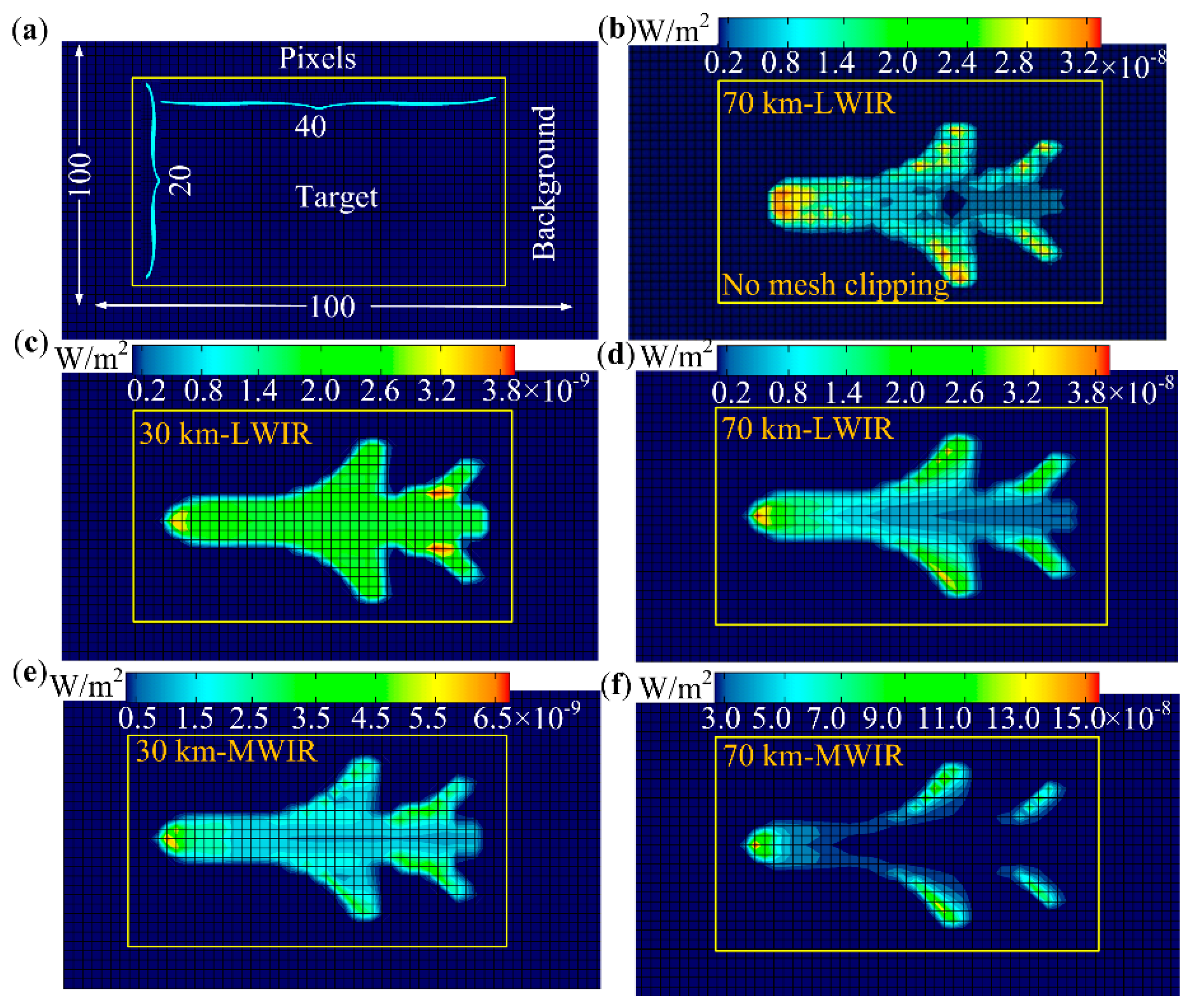
To display an enlarged image, partial background regions are removed in Figure 18a. In order to get the images below the same detection distance, an assumed distance of R = 30 km was used in both the 30-km and 70-km cases. Figure 18b–f show the upward-view TIR images with α/2 = 0.05°. Figure 18b shows the result without the mesh clipping.
To analyze the TIR distribution for different observation angles, the computing point of H = 70 km was selected. Figure 19 shows the TIR images of R = 70 km at α/2 = 0.01° and α/2 = 0.1°. Imaging was calculated in the front (θ = 90°, φ = 0°) and oblique-side (θ = 90°, φ = 135°) views. The upper left corner of the figure shows plots of the images at α/2 = 0.1°, and the right side of the figure presents the ratio of the peak intensity at α/2 = 0.1° to that at α/2 = 0.01°. It can be seen from Figure 19 that the image nearly became a point when the FOV increased to α/2 = 0.1°.
Figure 20 shows the peak intensity profiles of the TIR image at α/2 = 0.01° for different trajectory points. All calculations were performed on the assumption that R = H. The corresponding images within the MWIR and LWIR bands are illustrated at the top and bottom of the figure, respectively.
5. Discussion
The flow field contours of Figure 8 show that the high-temperature region of the surface occurred mainly at the windward surface of the nose and wing leading edges, and the temperature peak reached 2110 K in the 70-km case and 560 K in the 30-km case. In fluid regions, a distinct thermal nonequilibrium effect appeared in the case of 70 km, but these regions, appearing in the shock layer around the nose, were small. The mass fraction of NO generated by air dissociation was as high as 0.35. In the 30-km case, the aerodynamic temperature was drastically reduced in comparison with the 70-km case, and the flow was in thermal equilibrium.
In the top-view observation, the radiation of both the overall wake flows and most parts of the shock layer could be observed. It was demonstrated that the peak intensity radiation of the gases occurred mainly at the 2.7-μm (H2O), 4.3-μm (CO2,) and 5.3-μm (NO) bands. The spectrum of the surface radiation was smooth, and its peak intensity could be found around the short-wavelength region. A comparison of the radiation intensity between in Figure 10a and Figure 10b indicates that the gas radiance was at least one order of magnitude lower than that of the surface.
From Figure 11, it can be found that the MWIR radiance was lower than the LWIR for the 30-km case, but this phenomenon was reversed for the 70-km case. These two computational cases were significantly different for the MWIR radiance. There were four high-intensity areas in the case of 30 km and two in the 70-km case. This can be explained by the fact that the peak wavelength of the surface emission (in accordance with Planck’s law of gray-body radiation) moved toward the shorter wavelength as the temperature increased. The peak intensity did not occur in the front (θ = 90°, φ = 0°) or top (θ = 0°, φ = 90°) view, but in the oblique-side (θ = 22.5°, φ = 67.5° or φ = 337.5°) view. It can be observed that the two profiles intersected at the altitude of 35 km, which was the characteristic altitude Hc that separated the LWIR strong-emission regime (SER) and the MWIR SER.
In Figure 13, several phenomena can clearly be observed. Firstly, the MDR of the LWIR band was larger than that of the MWIR band at altitudes below 50 km (B-zone), which was a strong receiving regime (SRR) in the LWIR band, compared to the results shown in Figure 12, in which the characteristic altitude was shifted back by 15 km. Secondly, the target could not be detected at altitudes below 30 km using the MWIR band, which was a blind region (A-zone). In this figure, the gray dotted line indicates that the MDR was below the flight altitude H. Thirdly, there was an equivalent zone between 50 km and 60 km (C-zone) where the MDR was almost identical in two bands. Lastly, the MDR of the LWIR band decreased after 60 km in altitude, resulting in the presence of an SRR in the MWIR band. This phenomenon was related to radiance features and atmospheric attenuation.
It can be observed from Figure 16 that the MDR increment had typical characteristics. In the 30-km case, the MDR increments for most angles were approximately distributed on an equivalent flat plane except for a small fluctuation. Figure 16a,c show a heel-shaped distribution due to a low MDR increment in the back view. This indicates that an increase in the detectivity could improve the MDR in low-altitude cases. In the 70-km case, Figure 16b shows a crater-shaped distribution of the MWIR band, which was significantly different from Figure 16a. The values in the center region were larger than those in the marginal regions of the contour. For the LWIR band in Figure 16d, there was a three-peak shape, which reveals that the increase in the detectivity could greatly improve the MDR in the back and front views for high-altitude cases.
From Figure 18, the mesh clipping treatment demonstrated an obvious improvement in the imaging. These images also show that the TIR distributions in the 70-km and 30-km cases were both significantly different, and the peak intensity at 70 km was at least one order of magnitude higher than that at 30 km. It is demonstrated in Figure 19 that a smaller FOV could contribute toward capturing the TIR characteristics, but it required a more sensitive detectivity due to the reduction in TIR intensity for a large FOV. It can be seen from Figure 20 that the peak intensity difference in the LWIR images was within one order of magnitude, whereas the difference varied greatly for the MWIR images. Furthermore, there was an intersection between the two profiles that was attributable to the detection distance and the target’s radiance. In addition, TIR features of the nose and flanges became pronounced as the altitude increased. For the LWIR images, the difference in intensity distribution was small above altitudes of 40 km.
6. Conclusions
To examine the detection range and TIR images of an Earth entry vehicle, a complete numerical model was developed by analyzing a ground-based IR detection system and the physical mechanism of the TIR radiation. The proposed model was established considering optical radiative properties, optics propagation, atmospheric attenuation, and TIR arrangements in the pixels. Computer simulations were performed using known parameters for flight conditions and the IR detection system. The simulation results indicated that the radiance was strongly dependent on the observation angle and the spectral band. For the MWIR and LWIR bands, there was a characteristic altitude at which a strong-emission regime was noted. The MDR increased and the characteristic altitude decreased as the detectivity of the detector increased. The improvement in the detectivity could increase the MDR approximately linearly at most observation angles of low altitudes, but the MDR could be greatly improved in high-altitude cases. The TIR images showed that the mesh clipping treatment led to an obvious improvement in the TIR distribution. For the same detection conditions, the difference in the peak intensity for different trajectory points was at least one order of magnitude in scale. In addition, a smaller FOV could contribute toward capturing the TIR characteristics, but it required more sensitive detectivity due to the reduction in TIR intensity. The MWIR TIR features became more pronounced as the altitude increased, and those in the LWIR images were more suitable for detecting the aircraft’s configuration.
In further work, a sensitivity study and an uncertainty estimate of the numerical simulation should be carried out. Also, a more refined photodetector model should be used for evaluations of the detectivity of the target, and the effect of weather conditions on infrared optical observability should be considered in future work.
Author Contributions
Conceptualization, Q.N. and X.M.; methodology, Q.N.; software, Q.N.; validation, Q.N., X.M., and Z.H.; writing—original draft preparation, Q.N.; writing—review and editing, Q.N., Z.H., and S.D.; project administration, Q.N.; funding acquisition, S.D.
Funding
This research was funded by the National Nature Science Foundation of China, grant number 51576054.
Acknowledgments
We are grateful to Zhenhua Wang for help with programming.
Conflicts of Interest
The authors declare no conflict of interest.
Nomenclature
| A0 | pupil area of the objective lens system, m2 |
| Ad | pixel area of the detector, m2 |
| Ai,j,k | visible area of the kth surface element in the i × j pixel, m2 |
| At | effective radiation area of the target surface, m2 |
| c | speed of light, 2.99979 × 10⁸ m/s |
| C1, C2 | first and second radiation constants |
| d | degeneracy factors for state |
| D*(λ) | normalized system detectivity |
| El | energy of the lower state |
| Δf | frequency bandwidth of the detector circuitry |
| Frot | term value of rotational state |
| g | photoconductive gain |
| Gvib | term value of vibrational state |
| h | Planck constant, 6.6206896 × 10⁻³⁴ J·s |
| kB | Boltzmann constant, 1.38064852 × 10⁻²³ J·K−1 |
| I | radiation intensity, W/(sr·m2·μm) |
| M | number of segments in optical path |
| N | number density of species |
| ni | outward normal of the target surface element Ai |
| P | spectrum intensity arrived at the detector, W/(sr·μm) |
| Q(T) | partition function |
| R | distance between the target and the detector, m |
| q | irradiance received by each detector pixel, W/m2 |
| s | position |
| s | optical path vector |
| S(Tref) | line intensity under the standard condition |
| Vi,p | pth vertex of the element Ai |
| Greek | |
| η | wave number, cm−1 |
| Φ | line shape function |
| ε | emissivity |
| λ | wavelength, μm |
| τ(λ,R) | atmospheric transmittance with a distance of R |
| τ0(λ) | spectral transmittance of the optical system |
| Subscript | |
| u, l | upper and lower limits of spectral band |
| tar | target |
| bg | background |
| a | atmospheric air |
| s | surface of aircraft |
Abbreviation
| ASL | above sea level |
| AOA | angle of attack |
| CFD | computational fluid dynamics |
| FVM | finite volume method |
| FOV | field of view |
| HYTHIRM | hypersonic thermodynamic IR measurements |
| LOS | line-of-sight |
| LWIR | long-wavelength infrared |
| MDR | maximum detecting range |
| non-LTE | local thermodynamic nonequilibrium |
| NEFD | noise equivalent flux density |
| OTV | orbital test vehicle |
| RTE | radiative transfer equation |
| TIR | thermal infrared |
| SRC | sample return capsule |
| SNR | signal-to-noise ratio |
| SRR | strong receiving region |
| STS | space transportation system |
References
- Sziroczak, D.; Smith, H. A review of design issues specific to hypersonic flight vehicles. Prog. Aerosp. Sci. 2016, 84, 1–28. [Google Scholar] [CrossRef] [Green Version]
- Grantz, A. X-37B orbital test vehicle and derivatives. In Proceedings of the AIAA SPACE 2011 Conference & Exposition, Long Beach, CA, USA, 27–29 September 2011; p. 7315. [Google Scholar]
- Stark, B.; Smith, B.; Chen, Y. Survey of thermal infrared remote sensing for Unmanned Aerial Systems. In Proceedings of the 2014 International Conference on Unmanned Aircraft Systems (ICUAS), Orlando, FL, USA, 27–30 May 2014; pp. 1294–1299. [Google Scholar]
- Gong, M.; Guo, R.; He, S.; Wang, W. IR radiation characteristics and operating range research for a quad-rotor unmanned aircraft vehicle. Appl. Opt. 2016, 55, 8757–8762. [Google Scholar] [CrossRef]
- Niu, Q.; He, Z.; Dong, S. Prediction of shock-layer ultraviolet radiation for hypersonic vehicles in near space. Chin. J. Aeronaut. 2016, 29, 1367–1377. [Google Scholar] [CrossRef] [Green Version]
- Niu, Q.; Yuan, Z.; Dong, S.; Tan, H. Assessment of nonequilibrium air-chemistry models on species formation in hypersonic shock layer. Int. J. Heat Mass Transf. 2018, 127, 703–716. [Google Scholar] [CrossRef]
- Bonin, J.; Mundt, C. Full Three-Dimensional Monte Carlo Radiative Transport for Hypersonic Entry Vehicles. J. Spacecr. Rocket. 2018, 56, 1–9. [Google Scholar] [CrossRef]
- Rao, A.G.; Mahulikar, S.P. Effect of atmospheric transmission and radiance on aircraft infared signatures. J. Aircr. 2005, 42, 1046–1054. [Google Scholar] [CrossRef]
- Mahulikar, S.P.; Sonawane, H.R.; Rao, G.A. Infrared signature studies of aerospace vehicles. Prog. Aerosp. Sci. 2007, 43, 218–245. [Google Scholar] [CrossRef]
- Baranwal, N.; Mahulikar, S.P. Aircraft engine’s infrared lock-on range due to back pressure penalty from choked convergent nozzle. Aerosp. Sci. Technol. 2014, 39, 377–383. [Google Scholar] [CrossRef]
- Pan, X.; Wang, X.; Wang, R.; Wang, L. Infrared radiation and stealth characteristics prediction for supersonic aircraft with uncertainty. Infrared Phys. Technol. 2015, 73, 238–250. [Google Scholar] [CrossRef]
- Huang, W.; Ji, H. Effect of environmental radiation on the long-wave infrared signature of cruise aircraft. Aerosp. Sci. Technol. 2016, 56, 125–134. [Google Scholar] [CrossRef]
- Beier, K.; Gemperlein, H. Simulation of infrared detection range at fog conditions for enhanced vision systems in civil aviation. Aerosp. Sci. Technol. 2004, 8, 63–71. [Google Scholar] [CrossRef]
- Wang, K.; Dickinson, R.E. Global atmospheric downward longwave radiation at the surface from ground-based observations, satellite retrievals, and reanalyses. Rev. Geophys. 2013, 51, 150–185. [Google Scholar] [CrossRef]
- Horvath, T.J.; Cagle, M.F.; Gibson, D. Remote observations of reentering spacecraft including the space shuttle orbiter. IEEE Aerosp. Conf. 2013. [Google Scholar] [CrossRef]
- Spisz, T.S.; Taylor, J.C.; Kennerly, S.W.; Osei-Wusu, K.; Gibson, D.M.; Horvath, T.J.; Zalameda, J.N.; Kerns, R.V.; Shea, E.J.; Mercer, C.D. Processing ground-based near-infrared imagery of space shuttle re-entries. In Proceedings of Thermosense: Thermal Infrared Applications XXXIV; Proc. SPIE: Baltimore, MD, USA, 2012; p. 83540G. [Google Scholar]
- Horvath, T.J.; Rufer, S.J.; Schuster, D.M.; Mendeck, G.F.; Oliver, A.B.; Schwartz, R.J.; Verstynen, H.A.; Mercer, C.D.; Tack, S.; Ingram, B. Infrared Observations of the Orion Capsule During EFT-1 Hypersonic Reentry. In Proceedings of the AIAA Aviation and Aerospace Forum and Exposition, Washington, DC, USA, 13 June 2016; pp. 1–23. [Google Scholar]
- Schuster, D.M.; Horvath, T.J.; Schwartz, R.J. Remote Imaging of Exploration Flight Test-1 (EFT-1) Entry Heating Risk Reduction; Report: NASA/TM-2016-219214; NASA Langley Research Center: Hampton, VA, USA, 1 June 2016.
- Snively, J.B.; Taylor, M.J.; Jenniskens, P.; Winter, M.W.; Kozubal, M.J.; Dantowitz, R.F.; Breitmeyer, J. Near-Infrared Spectroscopy of Hayabusa Sample Return Capsule Reentry. J. Spacecr. Rocket. 2014, 51, 424–429. [Google Scholar] [CrossRef]
- Huang, F.; Wang, Y.; Shen, X.; Li, G.; Yan, S. Analysis of space target detection range based on space-borne fisheye imaging system in deep space background. Infrared Phys. Technol. 2012, 55, 475–480. [Google Scholar] [CrossRef]
- Zhao, Y.; Wu, P.; Sun, W. Calculation of infrared system operating distance by spectral bisection method. Infrared Phys. Technol. 2014, 63, 198–203. [Google Scholar] [CrossRef]
- Ren, K.; Tian, J.; Gu, G.; Chen, Q. Operating distance calculation of ground-based and air-based infrared system based on Lowtran7. Infrared Phys. Technol. 2016, 77, 414–420. [Google Scholar] [CrossRef]
- Suzuki, T.; Fujita, K.; Ando, K.; Sakai, T. Experimental study of graphite ablation in nitrogen flow. J. Thermophys. Heat Transf. 2008, 22, 382–389. [Google Scholar] [CrossRef]
- Lemal, A.; Jacobs, C.; Perrin, M.-Y.; Laux, C.; Tran, P.; Raynaud, E. Prediction of nonequilibrium air plasma radiation behind a shock wave. J. Thermophys. Heat Transf. 2015, 30, 197–210. [Google Scholar] [CrossRef]
- Mikula, D.; Holthaus, M.; Jensen, T.; Kubo, D.; Redgate, M. X-37 Flight Demonstrator system safety program and challenges. In Proceedings of the Space 2000 Conference and Exposition, Long Beach, CA, USA, 19–21 September 2000; p. 5073. [Google Scholar]
- Sarma, G. Physico–chemical modelling in hypersonic flow simulation. Prog. Aerosp. Sci. 2000, 36, 281–349. [Google Scholar] [CrossRef]
- Felton, M.; Gurton, K.; Pezzaniti, J.; Chenault, D.; Roth, L. Measured comparison of the crossover periods for mid-and long-wave IR (MWIR and LWIR) polarimetric and conventional thermal imagery. Opt. Express 2010, 18, 15704–15713. [Google Scholar] [CrossRef] [PubMed]
- Roe, P.L. Approximate Riemann solvers, parameter vectors, and difference schemes. J. Comput. Phys. 1981, 43, 357–372. [Google Scholar] [CrossRef]
- Yee, H.C. On Symmetric and Upwind TVD Schemes; NASA-TM-88325; NASA Langley Research Center: Washington, DC, USA, 1985. [Google Scholar]
- Khodabakhsh, A.; Ramaiah-Badarla, V.; Rutkowski, L.; Johansson, A.C.; Lee, K.F.; Jiang, J.; Mohr, C.; Fermann, M.E.; Foltynowicz, A. Fourier Transform and Vernier Spectroscopy with a Mid-Infrared Optical Frequency Comb. Proc. Opt. Nanostruct. Adv. Mater. Photovolt. 2016, 41, 2541–2544. [Google Scholar]
- Cadiou, E.; Dherbecourt, J.-B.; Raybaut, M.; Gorju, G.; Melkonian, J.-M.; Godard, A.; Pelon, J. Multiple-Species DIAL for H2O, CO2, and CH4 remote sensing in the 1.98–2.30 µm range. In Proceedings of the Laser Applications to Chemical, Security and Environmental Analysis, Orlando, FL, USA, 25–28 June 2018; p. LTu5C.5. [Google Scholar]
- Park, C. Nonequilibrium Hypersonic Aerothermodynamics; John Wiley & Sons: New York, NY, USA, 1989. [Google Scholar]
- Gamache, R.R.; Roller, C.; Lopes, E.; Gordon, I.E.; Rothman, L.S.; Polyansky, O.L.; Zobov, N.F.; Kyuberis, A.A.; Tennyson, J.; Yurchenko, S.N. Total internal partition sums for 166 isotopologues of 51 molecules important in planetary atmospheres: Application to HITRAN2016 and beyond. J. Quant. Spectrosc. Radiat. Transf. 2017, 203, 70–87. [Google Scholar] [CrossRef] [Green Version]
- Rothman, L.; Gordon, I.; Barber, R.; Dothe, H.; Gamache, R.; Goldman, A.; Perevalov, V.; Tashkun, S.; Tennyson, J. HITEMP, the high-temperature molecular spectroscopic database. J. Quant. Spectrosc. Radiat. Transf. 2010, 111, 2139–2150. [Google Scholar] [CrossRef]
- Banwell, C.N.; McCash, E.M. Fundamentals of Molecular Spectroscopy; McGraw-Hill: New York, NY, USA, 1994; Volume 851. [Google Scholar]
- Sparrow, E.M. Radiation Heat Transfer; Routledge: New York, NY, USA, 2018. [Google Scholar]
- Olivero, J.J.; Longbothum, R. Empirical fits to the Voigt line width: A brief review. J. Quant. Spectrosc. Radiat. Transf. 1977, 17, 233–236. [Google Scholar] [CrossRef]
- Niu, Q.; Yang, S.; He, Z.; Dong, S. Numerical study of infrared radiation characteristics of a boost-gliding aircraft with reaction control systems. Infrared Phys. Technol. 2018, 92, 417–428. [Google Scholar] [CrossRef]
- Fetter, S.; Sessler, A.M.; Cornwall, J.M.; Dietz, B.; Frankel, S.; Garwin, R.L.; Gottfried, K.; Gronlund, L.; Lewis, G.N.; Postol, T.A. Countermeasures: A Technical Evaluation of the Operational Effectiveness of the Planned US National Missile Defense System; Union of Concerned Scientist: Cambridge, MA, USA, 2000. [Google Scholar]
- Berk, A.; Bernstein, L.S.; Robertson, D.C. MODTRAN: A Moderate Resolution Model for LOWTRAN; Spectral Sciences Inc.: Burlington, MA, USA, 1987. [Google Scholar]
- Qinglin, N.; Zhichao, Y.; Biao, C.; Shikui, D. Infrared radiation characteristics of a hypersonic vehicle under time-varying angles of attack. Chin. J. Aeronaut. 2019, 32, 861–874. [Google Scholar]
- Ferrero, P.; D’Ambrosio, D. A numerical method for conjugate heat transfer problems in hypersonic flows. In Proceedings of the 40th Thermophysics Conference, Seattle, DC, USA, 23–26 June 2008; p. 4247. [Google Scholar]
- Mallet, M.; Periaux, J.; Rostand, P.; Stoufflet, B. Validation of aerodynamic simulation methods for Hermes spaceplane and future hypersonic vehicles. In Proceedings of the 4th Symposium on Multidisciplinary Analysis and Optimization, Cleveland, OH, USA, 21–23 September 1992. [Google Scholar]
- Hao, J.; Wang, J.; Lee, C. Numerical study of hypersonic flows over reentry configurations with different chemical nonequilibrium models. Acta Astronaut. 2016, 126, 1–10. [Google Scholar] [CrossRef]
- Levin, D.A.; Candler, G.V.; Limbaugh, C.C. Multispectral shock-layer radiance from a hypersonic slender body. J. Thermophys. Heat Transf. 2000, 14, 237–243. [Google Scholar] [CrossRef]
- Ozawa, T.; Garrison, M.B.; Levin, D.A. Accurate molecular and soot infrared radiation model for high-temperature flows. J. Thermophys. Heat Transf. 2007, 21, 19–27. [Google Scholar] [CrossRef]
- Richter, R.; Fries, J. Radiometric analysis of infrared sensor performance. Appl. Opt. 1988, 27, 4771–4776. [Google Scholar] [CrossRef] [PubMed]
- Alexeenko, A.; Gimelshein, N.; Levin, D.; Collins, R.; Rao, R.; Candler, G.; Gimelshein, S.; Hong, J.; Schilling, T. Modeling of flow and radiation in the Atlas plume. J. Thermophys. Heat Transf. 2002, 16, 50–57. [Google Scholar] [CrossRef]
- Qinglin, N.; Zhihong, H.; Shikui, D. IR radiation characteristics of rocket exhaust plumes under varying motor operating conditions. Chin. J. Aeronaut. 2017, 30, 1101–1114. [Google Scholar]
- Niu, Q.; Duan, X.; Meng, X.; He, Z.; Dong, S. Numerical analysis of point-source infrared radiation phenomena of rocket exhaust plumes at low and middle altitudes. Infrared Phys. Technol. 2019, 99, 28–38. [Google Scholar] [CrossRef]
- Shao, C.; Nie, L.; Chen, W. Analysis of weakly ionized ablation plasma flows for a hypersonic vehicle. Aerosp. Sci. Technol. 2016, 51, 151–161. [Google Scholar] [CrossRef]
- Coudrain, C.; Bernhardt, S.; Caes, M.; Domel, R.; Ferrec, Y.; Gouyon, R.; Henry, D.; Jacquart, M.; Kattnig, A.; Perrault, P. SIELETERS, an airborne infrared dual-band spectro-imaging system for measurement of scene spectral signatures. Opt. Express 2015, 23, 16164–16176. [Google Scholar] [CrossRef] [Green Version]
- Shibata, Y.; Nagasawa, C.; Abo, M. Development of 1.6 µm DIAL using an OPG/OPA transmitter for measuring atmospheric CO2 concentration profiles. Appl. Opt. 2017, 56, 1194–1201. [Google Scholar] [CrossRef]
- Meng, L.; Fix, A.; Wirth, M.; Høgstedt, L.; Tidemand-Lichtenberg, P.; Pedersen, C.; Rodrigo, P.J. Upconversion detector for range-resolved DIAL measurement of atmospheric CH4. Opt. Express 2018, 26, 3850–3860. [Google Scholar] [CrossRef]
Figure 1.
Diagrammatic sketch of orbital test vehicle (OTV) thermal infrared (TIR) observation. Atmospheric transmittance (gray) within the wavelengths of 0.4–14 μm at a low altitude is shown in the lower left corner. The flight path of the OTV and altitude-varying thermal and chemical properties are shown in the lower right corner. The variations of density and temperature with altitude are normalized using the corresponding above sea level (ASL) conditions.

Figure 2.
Sketch map of mesh clipping: (a) invisible elements caused by the obtuse angle between the line of sight (LOS) and its outer normal vector; (b) invisible elements caused by occlusion of other elements; (c) pixel array and relation between sensor pixel and target elements imaging; (d) distribution of intersection points in mesh clipping; (e) vertex sequence in a clockwise arrangement; (f) general position relationship between the target element and pixels.

Figure 3.
Flow chart of the calculation.

Figure 4.
Validation of the surface temperature and main flow field parameters: (a) surface temperature along the body at t = 60 s for the double-cone experiment in the L2K wind tunnel at DLR (German Aerospace Center) Köln; (b) flow field parameters of translational–rotational temperature (T), vibrational–electronic temperature (Tve), and mass fraction of dissociation product NO along the stagnation line for ELECTRE vehicle.

Figure 5.
Comparison of spectral radiance between calculated and reference data: (a) spectrum of H2O; (b) spectrum of CO2; (c) spectrum of NO.
Figure 5.
Comparison of spectral radiance between calculated and reference data: (a) spectrum of H2O; (b) spectrum of CO2; (c) spectrum of NO.

Figure 6.
Validation of infrared optical observability: (a) observation schematic diagram of the ground-based sensor for Atlas rocket exhaust plume; (b) comparison of the spectrum received by the sensor between computed and reference results.
Figure 6.
Validation of infrared optical observability: (a) observation schematic diagram of the ground-based sensor for Atlas rocket exhaust plume; (b) comparison of the spectrum received by the sensor between computed and reference results.

Figure 7.
Grid distribution of OTV: fluid computational domain consisting of outlet (red), symmetry plane (green), and far-field and inlet (blue) boundaries. The partially enlarged detail at the top right of the figure shows the structure computational domain.
Figure 7.
Grid distribution of OTV: fluid computational domain consisting of outlet (red), symmetry plane (green), and far-field and inlet (blue) boundaries. The partially enlarged detail at the top right of the figure shows the structure computational domain.

Figure 8.
Contours of flow field parameters: (a) translational–rotational (upper) and vibrational–electronic (lower) temperatures in the 70-km case; (b) mass fraction of NO in the 70-km case; (c) translational–rotational (upper) and vibrational–electronic (lower) temperatures in the 30-km case; (d) surface temperatures in the 30-km (left) and 70-km (right) cases.

Figure 9.
(a–d) Profiles of radiation intensity in two typical detection surfaces.

Figure 10.
Spectrum distributions in the top view (θ1 = 0°) in the 50-km and 70-km cases: (a) gas radiance; (b) surface radiance.
Figure 10.
Spectrum distributions in the top view (θ1 = 0°) in the 50-km and 70-km cases: (a) gas radiance; (b) surface radiance.

Figure 11.
TIR contours: (a) medium-wavelength infrared (MWIR) in the 30-km case; (b) MWIR in the 70-km case; (c) long-wavelength infrared (LWIR) in the 30-km case; (d) LWIR in the 70-km case.
Figure 11.
TIR contours: (a) medium-wavelength infrared (MWIR) in the 30-km case; (b) MWIR in the 70-km case; (c) long-wavelength infrared (LWIR) in the 30-km case; (d) LWIR in the 70-km case.

Figure 12.
Comparison of maximum TIR radiance for different computing points.

Figure 13.
Maximum detector distance distributions: (a) MWIR for the 30-km case; (b) MWIR for the 70-km case; (c) LWIR for the 30-km case; (d) LWIR for the 70-km case.
Figure 13.
Maximum detector distance distributions: (a) MWIR for the 30-km case; (b) MWIR for the 70-km case; (c) LWIR for the 30-km case; (d) LWIR for the 70-km case.

Figure 14.
Maximum detection range (MDR) profiles for different test points. There are four typical zones: blind region (A-zone), LWIR strong receiving region (SRR) (B-zone), equivalent zone (C-zone), and MWIR SRR (D-zone).
Figure 14.
Maximum detection range (MDR) profiles for different test points. There are four typical zones: blind region (A-zone), LWIR strong receiving region (SRR) (B-zone), equivalent zone (C-zone), and MWIR SRR (D-zone).

Figure 15.
Maximum improve distance for different test points.

Figure 16.
MDR increments: (a) MWIR for the 30-km case; (b) MWIR for the 70-km case; (c) LWIR for the 30-km case; (d) LWIR for the 70-km case.
Figure 16.
MDR increments: (a) MWIR for the 30-km case; (b) MWIR for the 70-km case; (c) LWIR for the 30-km case; (d) LWIR for the 70-km case.

Figure 17.
Profiles of MDR maximum increments.

Figure 18.
TIR images at an artificial detecting distance R = 30 km: (a) Pixel arrangement of target and background regions; (b) LWIR image without mesh clipping for 70-km case; (c) LWIR image for 30-km case; (d) LWIR image for 70-km case; (e) MWIR image for 30-km case; (f) MWIR image for 70-km case.

Figure 19.
TIR images of two typical observation angles for the 70-km case: (a) MWIR at φ = 0°, θ = 90°; (b) LWIR at φ = 0°, θ = 90°; (c) MWIR at φ = 135°. θ = 90°; (d) LWIR at φ = 135°, θ = 90°.
Figure 19.
TIR images of two typical observation angles for the 70-km case: (a) MWIR at φ = 0°, θ = 90°; (b) LWIR at φ = 0°, θ = 90°; (c) MWIR at φ = 135°. θ = 90°; (d) LWIR at φ = 135°, θ = 90°.

Figure 20.
Profiles of peak intensity and TIR images for different computing points.


Table 1.
Freestream conditions at computing trajectory points.
| Parameter | Values | ||||||
|---|---|---|---|---|---|---|---|
| h, km | 10 | 20 | 30 | 40 | 50 | 60 | 70 |
| p∞, Pa | 26,500 | 5529 | 1197 | 287 | 79 | 22 | 5 |
| T∞, K | 223 | 216 | 226 | 250 | 271 | 247 | 220 |
| u∞, km/s | 0.22 | 0.38 | 0.98 | 1.81 | 2.84 | 4.51 | 6.10 |
© 2019 by the authors. Licensee MDPI, Basel, Switzerland. This article is an open access article distributed under the terms and conditions of the Creative Commons Attribution (CC BY) license (http://creativecommons.org/licenses/by/4.0/).
Share and Cite
MDPI and ACS Style
Niu, Q.; Meng, X.; He, Z.; Dong, S. Infrared Optical Observability of an Earth Entry Orbital Test Vehicle Using Ground-Based Remote Sensors. Remote Sens. 2019, 11, 2404. https://doi.org/10.3390/rs11202404
AMA Style
Niu Q, Meng X, He Z, Dong S. Infrared Optical Observability of an Earth Entry Orbital Test Vehicle Using Ground-Based Remote Sensors. Remote Sensing. 2019; 11(20):2404. https://doi.org/10.3390/rs11202404
Chicago/Turabian StyleNiu, Qinglin, Xiaying Meng, Zhihong He, and Shikui Dong. 2019. "Infrared Optical Observability of an Earth Entry Orbital Test Vehicle Using Ground-Based Remote Sensors" Remote Sensing 11, no. 20: 2404. https://doi.org/10.3390/rs11202404
Note that from the first issue of 2016, this journal uses article numbers instead of page numbers. See further details here.