Satellite Remote Sensing of the Greenland Ice Sheet Ablation Zone: A Review

Abstract

The Greenland Ice Sheet is now the largest land ice contributor to global sea level rise, largely driven by increased surface meltwater runoff from the ablation zone, i.e., areas of the ice sheet where annual mass losses exceed gains. This small but critically important area of the ice sheet has expanded in size by ~50% since the early 1960s, and satellite remote sensing is a powerful tool for monitoring the physical processes that influence its surface mass balance. This review synthesizes key remote sensing methods and scientific findings from satellite remote sensing of the Greenland Ice Sheet ablation zone, covering progress in (1) radar altimetry, (2) laser (lidar) altimetry, (3) gravimetry, (4) multispectral optical imagery, and (5) microwave and thermal imagery. Physical characteristics and quantities examined include surface elevation change, gravimetric mass balance, reflectance, albedo, and mapping of surface melt extent and glaciological facies and zones. The review concludes that future progress will benefit most from methods that combine multi-sensor, multi-wavelength, and cross-platform datasets designed to discriminate the widely varying surface processes in the ablation zone. Specific examples include fusing laser altimetry, radar altimetry, and optical stereophotogrammetry to enhance spatial measurement density, cross-validate surface elevation change, and diagnose radar elevation bias; employing dual-frequency radar, microwave scatterometry, or combining radar and laser altimetry to map seasonal snow depth; fusing optical imagery, radar imagery, and microwave scatterometry to discriminate between snow, liquid water, refrozen meltwater, and bare ice near the equilibrium line altitude; combining optical reflectance with laser altimetry to map supraglacial lake, stream, and crevasse bathymetry; and monitoring the inland migration of snowlines, surface melt extent, and supraglacial hydrologic features.

1. Introduction

The Greenland Ice Sheet (GrIS) is the second-largest ice mass on earth. If the entire ice sheet were to melt, global sea level would rise by about seven meters [1]. At present, the GrIS is losing mass, consistent with its expected response to anthropogenic climate warming [2,3,4,5,6,7,8,9]. Its mass loss averaged –171 Gt yr⁻¹ between 1991 and 2015, equivalent to 0.47 ± 0.23 mm yr⁻¹ global eustatic sea level rise (SLR) [1]. The rate of SLR contribution accelerated to >1 mm yr⁻¹ during the latter half of this period with a maximum 1.2 mm contribution in the record melting year 2012 [1,10,11,12,13]. Since 2013, satellite gravimetry data suggest mass loss acceleration has stalled but remains negative with an average 0.69 mm yr⁻¹ SLR contribution during the 2012–2016 period [10,14,15]. Consequently, there is an urgent need to measure and diagnose changes in the GrIS mass balance, and satellite remote sensing is a powerful tool for this purpose [16].

The observed GrIS mass loss is being driven by both an increase in solid ice discharge (the physical movement of solid ice into surrounding oceans), and by decreasing surface mass balance (the surplus of surface meltwater runoff and evaporation over snowfall) [1,12,13,14,17,18,19,20,21]. About 60% of total mass loss since 1991 is explained by increased surface meltwater runoff from the ablation zone and lower elevation areas of the accumulation zone [1,22,23]. This increase is attributed in part to a prevailing pattern of warm, dry, clear-sky conditions during summer in (primarily) west Greenland associated with a persistently negative North Atlantic Oscillation (NAO) atmospheric circulation pattern [24,25]. Since about 2000, the NAO has exacerbated background regional warming of the surface air temperature, leading to enhanced surface melt, reduced summer snowfall, and larger areas of exposed bare ice that further enhance surface melt via melt-albedo feedbacks [14,23,24,25,26,27,28,29,30]. In the coming decades, regional warming is expected to drive a continued acceleration of surface meltwater runoff [2,3,4,5,6,7,8,9], whereas solid ice discharge is expected to decline relative to meltwater runoff as the marine-terminating ice sheet margins and outlet glaciers thin and retreat [14,18,31]. Consequently, surface processes in the ablation zone, particularly those that control the exposure and melting of bare ice, will play an enhanced role in determining the long-term GrIS mass balance [1,14,26,30,32]. Already, some 78–85% of the total liquid runoff produced from surface melting is generated in this zone, despite it covering ~22% of the ice sheet’s surface area, up from ~15% in the early 1960s [20,30,33,34,35].

Remote sensing plays a critical role in validating ice sheet mass balance and the associated SLR contribution [16]. For over three decades, satellite sensors operating in the visible, infrared, and microwave wavelengths of electromagnetic radiation have observed the GrIS [36]. The first spaceborne measurements of GrIS surface elevation were collected in the late 1970s by the National Aeronautics and Space Administration (NASA) Geodetic and Earth Orbiting Satellite-3 (GEOS-3), the NASA Seasat, and the US Navy Geosat oceanographic radar altimeters [37]. More recent radar altimetry missions useful for mapping ice sheet elevation change include the Geosat Follow-On (GFO), and the European Space Agency (ESA) European Remote-sensing Satellites 1 and 2 (ERS-1 and ERS-2), the Environmental Satellite (EnviSat), and the Cryosphere Satellite-2 (CryoSat-2). Radar altimetry now provides the longest record of GrIS volume change, owing to this steady progression of international radar altimeter missions extending to the present day [38].

Historically, ice sheet surface elevation retrieval accuracy from radar altimetry was limited by slope errors in the topographically-complex ablation zone, and uncertain signal penetration depth into snow and firn [39]. The laser altimeters onboard the NASA Ice, Cloud, and land Elevation Satellites 1 and 2 (ICESat-1 and ICESat-2) and the interferometric mode of the Ku-band (~13.9 GHz) radar altimeter onboard CryoSat-2 help redress these issues, and now provide sub-decimeter elevation change accuracy in the ablation zone [40,41]. In addition to new satellite laser and radar altimeters, gravimetry emerged in the early 2000s as a wholly novel remote sensing method for measuring the GrIS mass balance, with the first gravimetric measurements of the GrIS mass balance provided at ~400 km spatial scale by the NASA/German Aerospace Center twin Gravity Recovery and Climate Experiment (GRACE) in 2002 [36]. The GRACE-Follow On (GRACE-FO) satellite launched in May 2018 will continue the GRACE measurement time series for a planned ten years, and adds a new laser ranging interferometer that is expected to improve the satellite-to-satellite distance measurement relative to the GRACE microwave ranging system [42,43].

Optical satellite remote sensing provides the longest continuous spaceborne record of the changing GrIS surface. The first spaceborne photographic images of the GrIS were captured in the early 1960s by United States strategic reconnaissance satellites operated under the classified Corona program, followed by the unclassified Nimbus meteorological satellites launched by NASA in the mid-1960s [44,45,46]. The first multispectral images of GrIS surface reflectance were collected by the Multispectral Scanner (MSS) instrument on the Earth Resources Technology Satellite-1 (later renamed Landsat 1), launched by NASA in 1972 [47]. Multispectral imaging spectrometers now provide over three decades of ice and snow surface reflectance from which decadal time series of surface albedo are computed [48,49]. Together with thermal, synthetic aperture radar, and microwave scatterometer imagery, the entire GrIS ablation zone ice surface is imaged daily, and regions of unique ice composition (facies or zones) are mapped and monitored for change [35,50]. Crevasse fields, superimposed ice, seasonal snowlines, and “dark zones” of anomalously low albedo are all visible in satellite imagery [26,51,52,53,54]. These descriptive zones provide a framework for understanding the spatial organization and physical processes operating on the ablation zone ice surface and their temporal evolution, including surface meltwater presence, outcropping of entrained dust, and the inland migration of the seasonal snowline and supraglacial meltwater lakes [26,29,52,55,56]. Increasingly, ultra-high-resolution commercial satellite and drone imagery is used to recover unprecedented spatial detail, resolving surface features such as cryoconite holes and supraglacial rivers less than one meter in width [57,58,59].

Previous reviews of satellite remote sensing of glaciers and ice sheets exist [e.g., 46], including recent reviews focused on regional climate modeling of the GrIS surface mass balance [21,60]. Other reviews have focused on satellite altimetry and gravimetry of the combined Greenland and Antarctic ice sheet mass balance [36,61,62], the global land ice contribution to SLR during the satellite era [10], polar science applications of spaceborne wind scatterometers [63], satellite remote sensing of polar climate change [64], principles and theory of remote sensing methods for glaciology [65], remote sensing of Andean mountain glacier mass balance [66], optical remote sensing of Himalayan glaciers [67], glaciological applications of unmanned aerial vehicles [59], and many more specialized reviews of snow and ice optical or hydrologic properties with relevance to glaciological research [68,69,70,71,72,73,74,75,76,77,78,79,80,81]. To the authors’ knowledge, no review has focused specifically on satellite remote sensing the GrIS ablation zone, a small but critically important area of the ice sheet with unique physical processes and strong potential to expand in the coming years.

This review summarizes platforms, methods, and data products used for remote sensing of the GrIS ablation zone and some process-level discoveries that these data have produced. Because the ablation zone is defined as those areas where mass losses exceed gains, the review focuses exclusively on mass loss processes. The review is organized as follows: Section 2 defines key concepts relevant to the GrIS mass balance, surface mass balance, and energy balance. Section 3 reviews radar and laser (lidar) altimetry of GrIS surface elevation change. Section 4 reviews satellite measurements of the GrIS mass balance. Section 5 reviews optical remote sensing of the GrIS ablation zone surface reflectance and albedo. Section 6 reviews active and passive microwave, thermal, and multi-angular remote sensing of glaciological zones, surface melt extent, and surface roughness. Throughout the review, we provide suggestions for future research directions and opportunities in the context of present and future missions. Glossaries of satellite remote sensing sensors, platforms, and managing agencies discussed in this article are provided in Appendix A. The review concludes with a short synthesis and recommendations for future research.

2. Ice Sheet Mass Balance, Surface Mass Balance, and Energy Balance

Before reviewing satellite remote sensing of the GrIS ablation zone, we briefly define key concepts and terminology that are discussed throughout the review. Ice sheets and glaciers gain mass through snowfall and lose mass through sublimation, meltwater runoff, and solid ice discharge. Following Lenaerts et al. [21] and van den Broeke et al. [60], the mass balance $MB$ of an ice sheet is usually written as:

$$MB=SMB-D$$

(1)

where $SMB$ is surface mass balance and $D$ is solid ice discharged to surrounding oceans. The components of $MB$ are commonly expressed in units of mass per time (e.g., kg yr⁻¹ or Gt yr⁻¹), mass per unit area per time (e.g., kg m⁻² yr⁻¹), and mass per unit area per time normalized by density of liquid water (e.g., m water equivalent, m w.e. yr⁻¹) [21].

The $SMB$ is the sum of mass inputs and outputs at the ice surface:

$$SMB=P-E-E{R}_{ds}-R$$

(2)

where precipitation $P$ is the sum of liquid precipitation $P_{\mathit{liquid}}$ (e.g., rain) and solid precipitation $P_{\mathit{solid}}$ (e.g., snow), $E$ is the sum of evaporation and sublimation, $E{R}_{ds}$ is net snow erosion, and runoff $R$ is the sum of the liquid water balance:

$$R=M+P_{liquid}+CO-RF-RT$$

(3)

where $M$ is surface meltwater production, $CO$ is condensation, $RF$ is refreezing, and $RT$ is liquid water retention, e.g., water stored in lakes, aquifers, or under capillary tension in snow and ice. The GrIS ablation zone $SMB$ is dominated by $P_{\mathit{solid}}$ and $M$ with the remaining terms representing smaller but uncertain components [1,82,83,84,85]. The accumulation and ablation zones of the ice sheet are defined as those areas where the local $SMB$ > 0 and the local $SMB$ < 0, respectively. The equilibrium line altitude (ELA) separates the two zones where local $SMB$ = 0 [60].

The total change in ice sheet surface elevation over time (the quantity observed by spaceborne altimeters) is usually defined as:

$$\frac{dH}{dt}=\frac{SMB}{{\rho }_s}+\frac{BMB}{{\rho }_b}+\frac{D\prime }{{\rho }_i}+v_c+v_{br}$$

(4)

where $dH/dt$ is the total change in surface elevation (m yr⁻¹),$SMB$ (kg m⁻² yr⁻¹) is surface mass balance, ${\rho }_{\mathrm{s}}$ (kg m⁻³) is surface snow, firn, and/or ice density, $BMB$ (kg m⁻² yr⁻¹) is the change in basal mass balance, ${\rho }_{\mathrm{b}}$ (kg m⁻³) is basal ice density, $D\prime$ (kg m⁻² yr⁻¹) is the local change in ice mass due to ice dynamic motion, ${\rho }_i$ is solid ice density, $v_{\mathrm{c}}$ (m yr⁻¹) is vertical velocity due to snow and/or firn compaction, and $v_{\mathrm{br}}$ (m yr⁻¹) is vertical bedrock velocity (e.g., glacial isostatic adjustment) [86,87]. The vertical velocity terms contribute to $dH/dt$, but are not associated with change in $MB$.

Equation (4) is used to estimate volumetric changes in the polar ice sheets, and also to estimate $MB$. This requires correction for the vertical velocity terms and an estimate of ${\rho }_{\mathrm{s}}$, which for the ablation zone is typically taken as a constant value between 830 kg m⁻³ and 917 kg m⁻³ [88], whereas for snow and firn above the ELA, measured or modeled values of ${\rho }_{\mathrm{s}}$ are necessary to convert $dH/dt$ to $SMB$ [86]. In some cases, all but the first term on the right-hand side of Equation (4) can be neglected and the local $SMB$ can be inferred from remotely sensed $dH/dt$ [89].

The energy available for melting snow or ice is determined by the sum of positive and negative heat fluxes at the surface, referred to as the surface energy balance $SEB$ (W m⁻²):

$$\begin{gathered} SEB=S{W}_{NET}+L{W}_{NET}+SHF+LHF+G_S \\ \hspace{1em}\hspace{1em}\hspace{1em}\hspace{1em}\hspace{1em}\hspace{1em}\hspace{1em}=S{W}_{in}\left(1-\alpha \right)+L{W}_{in}-\sigma T_{sfc}^4+SHF+LHF+G_S \end{gathered}$$

(5)

where $SW$ and $LW$ are shortwave (solar) and longwave (terrestrial) radiation fluxes, $SHF$ and $LHF$ are the turbulent surface fluxes of sensible and latent heat (which are proportional to the aerodynamic surface roughness length, $\zeta$ (m⁻¹)), $G_{\mathrm{S}}$ is subsurface (conductive) heat flux, $\alpha$ is the broadband surface albedo, or the ratio of upwelling (reflected) solar radiation to downwelling (incoming) solar radiation ($S{W}_{\mathrm{up}}/S{W}_{\mathrm{in}}$), $\sigma$ is the Stefan Boltzmann constant (5.67 × 10⁻⁸ W m⁻² K⁻²), and $T_{\mathrm{sfc}}$ is the ice surface kinetic temperature. In Equation (4), all heat fluxes have units W m⁻² and are defined as positive toward the surface [60].

If $T_{\mathrm{sfc}}$ reaches the melting temperature of ice, positive $SEB$ provides melt energy $ME$ (W m⁻²) and liquid meltwater $M$ is produced. The dominant source of $ME$ for the GrIS is $S{W}_{\mathrm{NET}}$ [90]. Typical values of $\alpha$ are 0.9 for freshly fallen snow, 0.6 for melting snow, and 0.4 for bare glacier ice [73]. This wide variability in $\alpha$ demonstrates the critical role of albedo in modulating the $SEB$ and consequently $M$ in the GrIS ablation zone [26,29,30].

3. Ice Surface Elevation Change

The magnitude of GrIS $dH/dt$ and its spatio-temporal variability has been quantified for nearly four decades using spaceborne radar (Radio Detection and Ranging) altimetry [37,38,91,92,93,94,95], and since 2001, using spaceborne laser altimetry [96,97,98,99,100,101]. Recent advances in laser and radar altimeter precision and spatial resolution allow discrimination of $dH/dt$ in slower-flowing, land-terminating sectors of the GrIS ablation zone, principally caused by a change in $SMB$ rather than $D$ [102,103]. For the accumulation zone, regional climate models and firn compaction models are used to partition the component of $dH/dt$ caused by a change in $SMB$ from those caused by a change in firn density and $D$ [104,105]. The following subsections summarize spaceborne radar altimetry of the GrIS, providing a historical perspective that emphasizes major challenges and advances in the field, and identifies future opportunities for radar altimetry observations of the GrIS ablation zone.

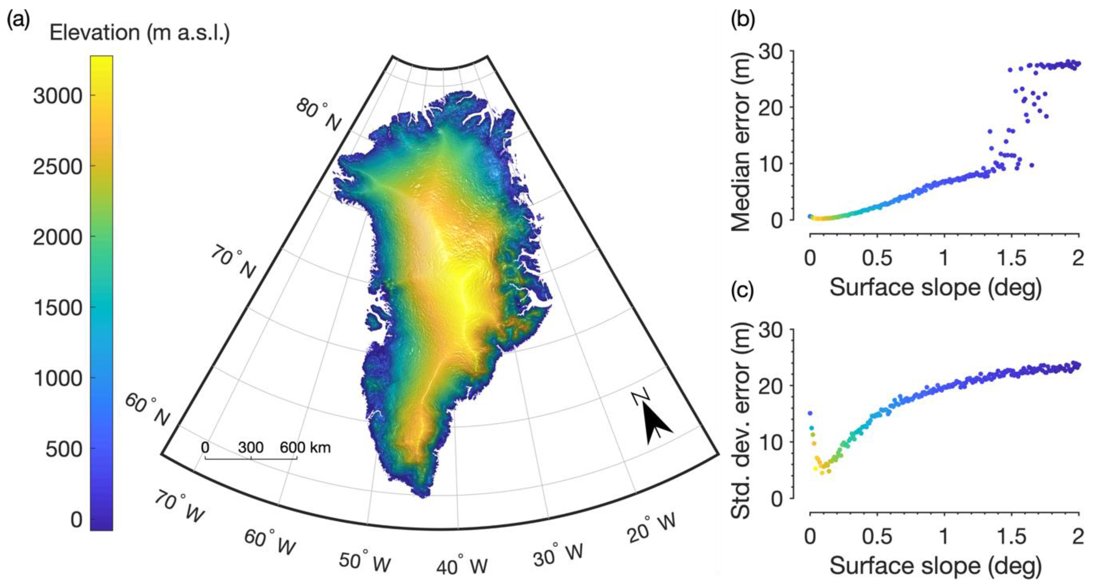
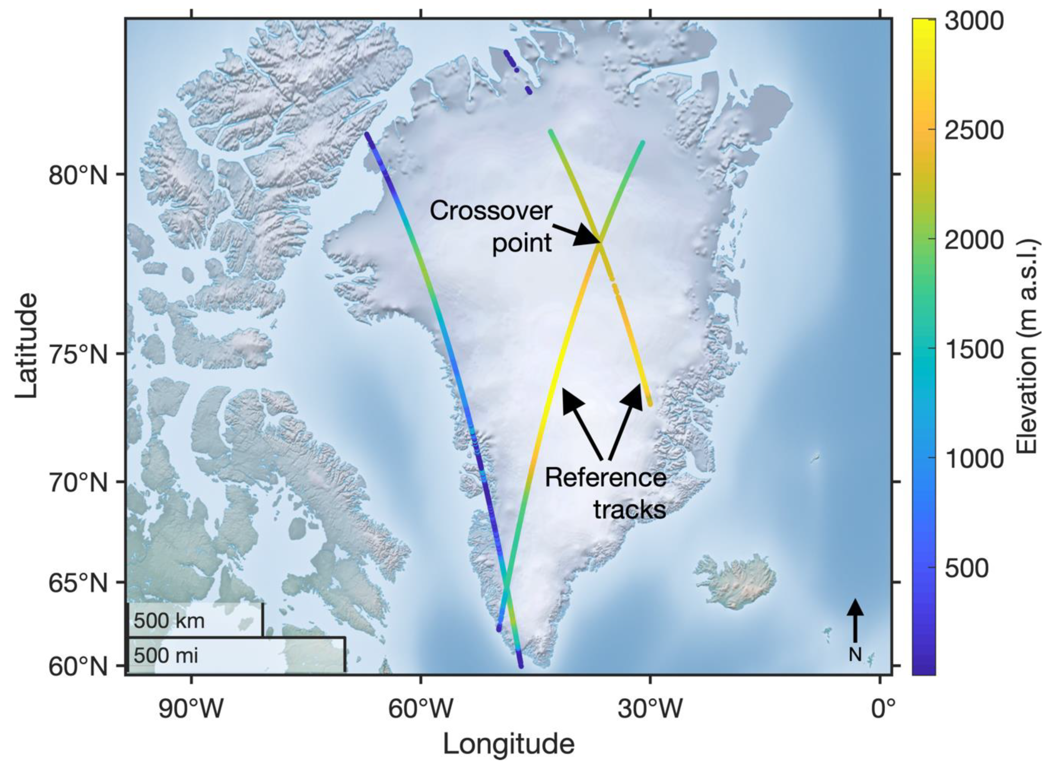
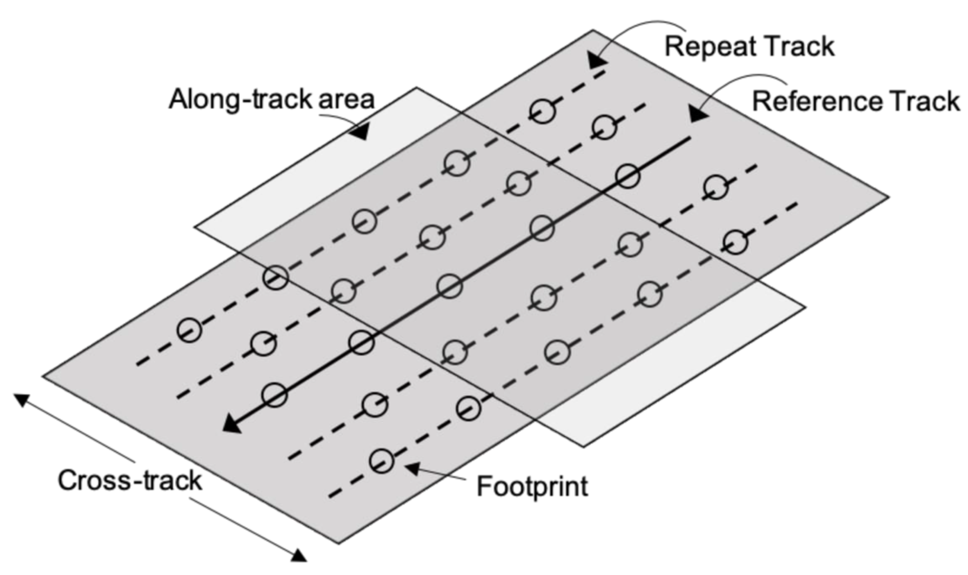
3.1. Radar Altimetry

Conventional radar altimeters are nadir pointing single-beam radars that transmit and receive tens to thousands of microwave pulses per second, yielding ground measurement footprint diameters on the order of 1–10 km posted at 0.3–0.6 km along-track spacing [39,106,107]. An estimate of $dH/dt$ is obtained by comparing measurements at crossover points, where an earlier satellite ground track intersects a later one [92]. Two critical factors affect the accuracy of radar altimeter elevation retrievals over ice sheets: (1) variation in topographic slope, which controls the average distance between the altimeter and the measured ground footprint surface [39,108,109], and (2) changes in the electrical permittivity of the ice sheet surface, which controls the reflection, transmission, and absorption of the microwave signal [110,111,112,113].

For typical radar altimeter frequencies (Ku-band ~13 GHz), solid ice and liquid water are highly reflective, whereas dry snow and firn are semi-transparent, with Ku-band penetration depths on the order of several meters [114,115]. Spatial and temporal variations in signal penetration depth caused by seasonal bare ice exposure, snow and firn densification, surface meltwater presence, and refreezing of meltwater introduce spurious height change signals that are poorly quantified for the GrIS but are estimated to exceed >0.50 m in some cases [116,117,118]. Variations in surface slope dominate radar altimeter accuracy in the topographically-complex bare-ice ablation zone, with slope-induced errors that exceed >20 m for slopes >1° [39,109,113]. The recent CryoSat-2 radar altimeter mission employs synthetic aperture radar (SAR) and interferometric synthetic aperture radar (InSAR) technologies, which decrease the effective along-track footprint diameter to the order 0.1–0.3 km and provide the cross-track slope from InSAR processing [93]. Together with denser orbital-track spacing and advances in waveform retracking, topographic mapping of ice sheet ablation zone areas is accurate to within a few meters on average, and $dH/dt$ to within sub-meter uncertainty relative to laser altimetry [93,119,120].

3.1.1. Radar Altimetry Sensors and Datasets

The first satellite altimeter measurements of surface topography for the Greenland Ice Sheet were made by the GEOS-3, Geosat, and Seasat oceanographic Ku-band altimeters (

Table 1. Summary of radar and laser altimeter remote sensing platforms, instruments, temporal coverage, observed wavelength, and managing agencies.

Platform *	Instrument Ŧ	Temporal Coverage	Observed Wavelength	Agency §,Ɣ
Radar altimeters
GEOS-3	ALT	1975–1978	13.9 GHz (Ku)	NASA
Seasat	ALT	1978 (110 days)	13.6 GHz (Ku)	NASA
Geosat	GRA	1985–1990	13.5 GHz (Ku)	DoD/NASA
ERS-1	RA	1991–2006	13.8 GHz (Ku)	ESA
ERS-2	RA-2	1995–2011	13.6 GHz (Ku), 3.2 GHz (S)	ESA
GFO	GFO-RA	1998–2008	13.5 GHz (Ku)	DoD/NASA
EnviSat	RA-2	2002–2012	13.6 GHz (Ku), 3.2 GHz (S)	ESA
CryoSat-2	SIRAL	2010–present	13.9 GHz (Ku)	ESA
SARAL	ALtiKa	2013–present	36 GHz (Ka)	ISRO/CNES
Sentinel-3A/B	SRAL	2016–present	13.6 GHz (Ku), 5.4 GHz (C)	ESA
Laser altimeters
ICESat	GLAS	2003–2009	1.064 μm, 0.532 μm	NASA
ICESat-2	ATLAS	2018–present	1.064 μm, 0.532 μm	NASA
Aircraft	ATM	1977–present	1.064 μm	NASA
Aircraft	LVIS	1998–present	1.064 μm	NASA
Aircraft	MABEL	2012–2014	1.064 μm, 0.532 μm	NASA

*,^Ŧ,^§ See Abbreviations at end of article for expanded acronyms. ^Ɣ Managing agencies are identified by the WMO OSCAR database (Table A1) and may not reflect joint collaborations.

) [37,91,106,121,122]. Their geographical coverage was limited to ±72°, but the data they collected showed it was possible to calculate volumetric changes in the polar ice sheets from space, providing proof of the concept for future polar-orbiting altimeters [92]. A first demonstration using GEOS-3, Geosat, and Seasat data found that for areas south of <72° N, the GrIS thickened by 23 ± 6 cm yr⁻¹ between 1978–1986, with enhanced snowfall in a warmer climate hypothesized to explain the observed thickening [123]. These early missions supported important developments in waveform retracking, slope correction, and physical and empirical models for subsurface volume scattering [106,108,111,124]. These corrections are critical for accurate elevation retrieval and reliable change detection [125,126]. For example, Davis et al. [127] used an improved geodetic model and an improved retracking model to reinterpret the earlier findings of Zwally et al. [92], finding a smaller 1.5 ± 0.5 cm yr⁻¹ thickening for the period 1978–1986 that highlighted the importance of slope- and signal penetration-correction.

The ESA European Remote-Sensing Satellite (ERS-1) carried the first polar-orbiting radar altimeter, extending coverage of the polar ice sheets to ±81.5° [95]. Together with the follow-on ERS-2 and EnviSat missions, these satellites provided near-complete GrIS coverage and 21 years of continuous data acquisition [38]. The first digital elevation model (DEM) spanning the entire GrIS surface was produced from combined ERS-1 and Geosat altimetry data, supplemented by stereo-photogrammetric and cartographic data sets, with pan-GrIS average accuracy of −0.33 ± 6.97 m [128,129]. ERS-1/2 altimetry data were used to discriminate thinning rates in the ablation zone (defined as <1500 m a.s.l.) of –2.0 ± 0.9 cm yr⁻¹ from accumulation zone (>1500 m a.s.l.) thickening of 6.4 ± 0.2 cm yr⁻¹ with an overall net thickening of 5.4 ± 0.2 cm yr⁻¹ for the period 1992–2003 [130]. To extend the temporal coverage and increase spatial measurement density, Khvorostovsky and Johannessen [131] developed an algorithm to merge ERS-1/2 and EnviSat datasets and detect and eliminate inter-satellite biases. For the period 1992–2008, their dataset suggests net thinning of the GrIS initiated around 2000, and accelerated between 2006–2008, with a thickening of 4.0 ± 0.2 cm yr⁻¹ above 1500 m a.s.l. and thinning of –7.0 ± 1.0 cm yr⁻¹ below 1500 m a.s.l. [94].

Conventional radar altimeters, such as the instruments included on ERS-1/2 and EnviSat, were optimized for detecting elevation over open oceans and low-gradient polar ice sheet interiors with mean accuracies typically of <0.2 m for ice sheet surface slopes <0.2° [39,109]. Elevation accuracy and $dH/dt$ uncertainty are much higher for the topographically complex ablation zone due to their large spatial measurement footprint and wide orbital track spacing, with slope errors >20 m for slopes >1^o and systematic biases over rough surfaces [39,95,109,132]. Careful processing has been used to discriminate ablation zone thinning rates using ERS-1/2 and EnviSat altimetry data, including repeat-track analysis, but the accuracy of these data and their process-based interpretation is ambiguous owing to the aforementioned slope errors and sparse spatial measurement density in the ablation zone [118,133,134,135].

The CryoSat-2 satellite (launched April 2010) provides continuity with ERS-1/2 and EnviSat, and employs SAR delay-Doppler along-track processing and interferometric cross-track processing [120,136]. CryoSat-2 is the first ESA radar altimeter dedicated to polar studies, with orbital coverage to ±88° and 1.6 km cross-track spacing at 70°. CryoSat-2 carries two Ku-band SAR/Interferometric Radar Altimeter (SIRAL) systems. SIRAL operates in three distinct modes depending on location: (1) low resolution mode (LRM) over open ocean and ice sheet interiors, (2) synthetic aperture radar mode (SAR) over sea ice and coastal regions, and (3) SAR interferometric mode (SARIn) over ice sheet margins. The SARIn mode employs two SAR instruments oriented across the satellite track. Interferometric phase processing of the dual waveforms provides a cross-track slope at ~0.3 km along-track resolution [137,138].

Over mild slopes (<1°), phase unwrapping [136] of CryoSat-2 interferometric data provides 5 km wide-swath elevation retrievals with two orders of magnitude more individual measurements per surface area than any prior radar altimeter [119,120,137]. The first spatially continuous swath DEMs were generated from CryoSat-2 data for areas of the Devon Ice Cap and western GrIS with ±3 m precision [119,137]. Swath processing provides information about within-swath topography that is not provided by traditional radar processing techniques. For example, Gray et al. [119] demonstrated a novel method for supraglacial lake water surface elevation retrievals in the ablation zone from CryoSat-2 swath retrievals and provided a detailed technical description of swath processing.

The SIRAL system nominally resolves $dH/dt$ to 3.3 cm yr⁻¹ near the ice sheet margins and 0.7 cm yr⁻¹ in the ice sheet interior, at a 104 km² and 106 km² spatial scale, respectively [138]. Using three years (2011–2014) of CryoSat-2 standard retrievals and an updated threshold retracking algorithm, a new pan-GrIS DEM was generated with a 3 ± 15 m elevation accuracy relative to ICESat over 80% of the GrIS and 5 ± 65 m accuracy over 90% of the GrIS (Figure 1) [93]. These data suggest reliable CryoSat-2 elevation retrievals remain limited to areas of the ablation zone with a surface slope <1.5^o (Figure 1). Elevation change from these data suggests a 2.5 factor increase in pan-GrIS volume loss (-375 ± 24 km³ yr⁻¹) compared with the ICESat (2003–2009) period, with large losses concentrated in the west and southeast marginal ablation zones [93]. A separate analysis of the same data combined with a firn density model found an equivalent mass loss of 269 ± 51 Gt yr⁻¹ [105].

Currently operating beyond its design lifetime, CryoSat-2 will be succeeded by the SAR Radar Altimeter (SRAL) onboard Sentinel-3A/B, and by the AltiKa Ka-band radar altimeter onboard the Satellite with ARgos and ALtiKa (SARAL) (Table 1). SARAL is a joint French Space Agency (CNES) and Indian Space Research Organisation (ISRO) oceanographic mission launched in 2013 with the secondary goal of monitoring polar ice sheet surface elevations [139]. SARAL has the same 35-day repeat orbit as EnviSat and ERS-1/2, but the AltiKa instrument operates at Ka-band (~36 GHz), thereby offering unique opportunities for cross-platform validation of prior Ku-band radar altimeters [140]. In particular, the Ka-band should improve diagnosis of Ku-band signal penetration bias, owing to its higher (~36 GHz) signal frequency with ~10 × lower theoretical penetration depth into dry snow relative to Ku-band, higher spatial resolution (~8 km footprint and 175 m along-track spacing), and higher pulse-repetition frequency [135,141,142,143]. SARAL also provides an independent record of ice sheet $dH/dt$. Using the 1 km ICESat DEM for the period 2003–2005 [144] as a baseline, data from SARAL-AltiKa for the period 2014–2016 was used to estimate a pan-GrIS volume loss rate of 247 km³ yr⁻¹, with the largest basin-scale volumetric decreases found in the north and northwest [145].

3.1.2. Current Challenges and Future Opportunities

Progress in waveform retracking and SAR/InSAR technology has improved radar altimetry performance over complex terrain, but retracking errors over rough surfaces and spatiotemporal variations in signal penetration depth remain important sources of uncertainty. Reliable performance in the ablation zone appears limited to areas with surface slope <1.5° (Figure 1), and signal penetration biases may exceed 0.5 m in the lower accumulation zone [116,118,119,147]. Nevertheless, radar altimetry provides the longest record of GrIS $dH/dt$, and two challenges stand out for leveraging this unique dataset: (1) homogenization of the inter-mission and cross-platform methods and datasets used to detect $dH/dt$ [133,148], and (2) better understanding of spatial and temporal changes in snow, firn, and ice permittivity caused by surface meltwater presence, meltwater percolation, and ice lens formation [116,147]. These challenges are closely related. For example, methods such as waveform smoothing, waveform model fitting, and optimal thresholding increase absolute accuracy, but at the expense of the homogenization required for statistical change detection [125,126,149]. In other cases, waveform retracking may mask real $dH/dt$ signals [150]. Similarly, real changes in snow and firn permittivity may introduce false $dH/dt$ signals, such as the apparent 56 ± 26 cm elevation increase attributed to ice lens formation in the percolation zone following the 2012 melt event [116]. Here, the SARAL-AltiKa Ka-band altimeter may provide new opportunities for diagnosing radar penetration bias and waveform interpretation. In addition, its replication of the ERS-1/2 and EnviSat repeat orbit will improve the statistical reliability of along-track change detection [140].

In contrast to the percolation zone, the ablation zone is typically conceptualized as homogenous solid ice with uniform electromagnetic properties. Ku-band backscatter over the bare ice ablation zone is dominated by surface scattering from the rough (and seasonally saturated) ice surface, but volume scattering has received little direct study and may be important over superimposed ice, seasonally-snow covered surfaces, or areas with multi-modal surface roughness distributions [151]. Penetration depths at C- and L-band exhibit an order of magnitude range over bare ice surfaces on the GrIS, possibly reflecting variations in ice thermal structure and surface roughness [152]. Similar comparisons at the Ku-band do not exist to our knowledge but could be facilitated by dual-frequency radar altimeters such as SRAL or RA-2, or by comparison with SARAL-AltiKa Ka-band altimetry (Table 1). Factors that affect bare ice microwave permittivity include its grain size, temperature, porosity, water content, crystal structure, and chemical and physical impurity content [153,154,155,156]. Although slope errors dominate elevation retrieval uncertainty in the ablation zone, seasonal and spatial variations in ablation zone surface properties and their effect on radar backscatter may be an overlooked source of uncertainty [117,135]. Conversely, this variation and its effect on waveform shape could provide new opportunities for understanding the ablation zone, such as detecting water surface elevation change in supraglacial lakes, inferring changes in near-surface ice structure related to physical weathering of solid ice, or estimating seasonal snow thickness using a dual-frequency radar, as was recently demonstrated for Arctic sea ice using combined CryoSat-2 and SARAL-AltiKa retrievals [119,156,157].

At the ice-sheet scale, knowledge of snow, firn, and ice density is the main source of uncertainty for conversion between ice sheet volume change and mass change [36]. Density changes are caused by snow and firn compaction and by meltwater refreezing, which both affect waveform interpretation by changing the scattering properties of the snow and firn [105,116]. Field investigations suggest ice lenses are widespread in the percolation zone and have thickened in recent decades [20,158]. The vertical and horizontal distribution of meltwater percolation and refreezing is difficult to model and may not be accurately represented by regional climate models [158,159]. Although these features present challenges for $dH/dt$ detection, they also provide unique opportunities for characterizing snow and firn processes, including detection of extreme melt events, ice lens formation, and snow accumulation rates following ice lens formation [115].

3.2. Laser Altimetry

Laser altimeters use lidar (light detection and ranging) technology to measure the two-way travel time of narrow-beam monochromatic laser pulses transmitted between the altimeter and the earth’s surface. In contrast to radar altimetry, signal penetration in ice and snow is minimal at common lidar wavelengths (visible and near-infrared), and the narrow laser beam illuminates a much smaller ground area, which reduces slope errors over complex terrain [39,160]. The small laser footprint increases absolute accuracy but may also introduce uncertainty because interpolation between narrow footprints is needed to obtain spatially continuous elevations [99]. Laser altimeters are sensitive to atmospheric scattering and lack the all-weather capability of radar altimeters but are uniquely adept at measuring local surface elevation in the topographically complex ablation zone, allowing resolution of thinning rates at the scale of individual outlet glaciers and providing benchmark datasets for altimeter accuracy [97,161]. The following subsections summarize spaceborne laser altimetry of the GrIS, emphasizing the operational performance of ICESat, and future opportunities for laser altimetry observations of the GrIS ablation zone from the recently launched ICESat-2.

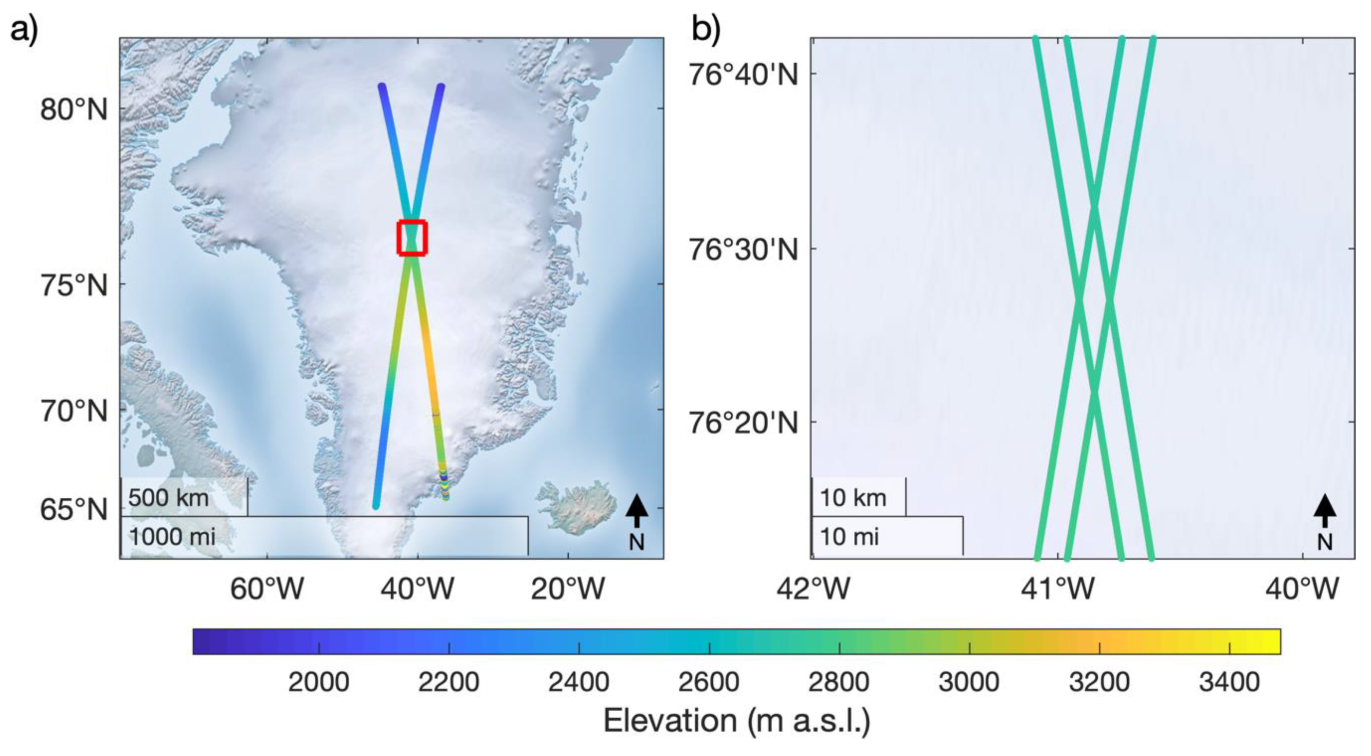
3.2.1. Laser Altimetry Sensors, Methods, and Datasets

The NASA Lidar In-Space Technology Experiment (LITE), flown on the Discovery Space Shuttle in September 1994, was the first spaceborne lidar [162]. The LITE was focused on the vertical structure of clouds and aerosols and provided operational proof of the concept. The NASA Geoscience Laser Altimeter System (GLAS) onboard the ICESat satellite (2003–2009) (Table 1) was the first spaceborne lidar designed for polar science. The GLAS transmitted short pulses of near infrared (1064 nm) light for surface altimetry and visible green light (532 nm) for vertical distribution of clouds and aerosols [101]. The ICESat mission was marked by several important innovations in polar altimetry, including unprecedented spatial resolution (70 m footprint, 172 m along-track spacing, and 3 cm vertical resolution), geographic coverage to ±86°, and the use of a narrow-beam 1064 nm laser which reduced sensitivity to both slope errors and signal penetration into snow and firn [163].

An important design objective of ICESat was to measure ice sheet surface elevation change over regions of high surface slope and complex topography, with primary mission objectives to measure spatially-averaged (104 km²) ice sheet surface elevation to <15 cm absolute accuracy and elevation change to <1.5 cm yr⁻¹ accuracy [36,101]. Field validation suggests operational absolute accuracy achieved 2 ± 3 cm for optimal conditions [164]. At-a-point measurement precision is ± 3 cm over the ice sheets and the repeat crossover measurement uncertainty is typically 10–15 cm [163,165], and up to 59 cm in regions of high surface slope [39]. Performance is affected by forward scattering of the return signal by intervening clouds, detector saturation, uncertain laser pointing angle, and laser transmit power decline [39,164,166].

The ICESat payload included three separate laser systems. Technical issues with the lasers prevented planned continuous operation, and instead, data collection took place during 18 separate campaigns [166,167]. Campaigns were designated by the laser system used and the campaign-specific orbital repeat frequency. For example, the first laser system operated for 38 days in an 8-day calibration and validation mode repeat frequency before it failed [167]. The second and third laser systems operated in campaign mode with a 91-day repeat frequency constituting individual campaigns ~33 days in length separated by 4–6 months. Inter-campaign range biases up to ~20 cm have been found [165,168]. The biases owe in part to a coding error in the ICESat signal processing algorithm that has since been corrected [168]. On-orbit and post-processing bias corrections were developed to compensate for orbital drift and systematic laser orientation (pointing) errors, but residual inter-campaign biases are an important measurement uncertainty in the ICESat data [86,165,169].

As with all spaceborne altimeters, the ICESat orbit followed ascending and descending orbital reference tracks with crossover reference points at the ascending and descending orbit intersections (Figure 2). Several factors affect the geolocation of ICESat ground footprints at repeat-track and crossover locations. These include orbital vibrations, orbital drift, random errors in ICESat’s laser orientation determination system, and declines in laser transmit power through time that modify the illuminated footprint diameter [164,167,170]. These factors produce both real and apparent deviations between illuminated ground tracks and reference tracks up to a few hundred meters [163,171]. Consequently, exact co-located repeat track and crossover point measurements are extremely rare, and spatial interpolation is required to recover $dH/dt$ at-a-point, which has become a central challenge for ICESat data interpretation [171]. To estimate pan-GrIS $dH/dt$, an additional spatial interpolation of the point $dH/dt$ estimates is typically performed, which is complicated by temporal differences among the point $dH/dt$ estimates e.g., [86].

As detailed by Felikson et al. [99], four methods have been developed to recover $dH/dt$ from ICESat data: (1) repeat tracks (RTs), (2) crossovers (XOs), (3) overlapping footprints (OFPs), and (4) surface fitting methods, such as triangulated irregular networks (TINs). The Surface Elevation Reconstruction and Change (SERAC) method [171] combines elements of RT and XO [99]. Alberti and Biscaro [172] summarize the ICESat orbital parameters in detail and describe a flexible algorithm for determining RT and XO points from them.

The XO method calculates $dH/dt$ at the ascending and descending orbital crossover points. The method was originally developed for radar altimetry and was expected to be the primary method for interpreting ICESat data [101]. The method was used to estimate a relative elevation accuracy for ICESat of 0.14–0.59 m depending on the surface slope [39]. Using ICESat XO points as reference values, absolute accuracies for ERS-1/2 and EnviSat radar retrievals are ~0.10–0.56 m for surface slopes <0.1°, but are 2.27 m on average and up to 30 m for surface slopes exceeding 0.7° [39]. These differences demonstrate the utility of laser altimetry for validating radar altimetry but also suggest caution when combining retrievals at discrete locations with high surface slopes and/or topographic variability c.f. [109].

The RT method calculates $dH/dt$ from repeat measurements at reference points along the reference tracks, which increases spatial measurement density and coverage relative to XO points (Figure 3) [173]. However, RT points are typically further apart than XO points, which may increase slope errors [99]. Owing to higher measurement density, the RT method has seen greater operational use than the XO method and is more appropriate for local or regional scale analysis [99]. The RT method was combined with Advanced Spaceborne Thermal Emission and Reflection Radiometer (ASTER) digital elevation model differencing, which together suggest an average volume loss in southeast Greenland of ~108 km³ yr⁻¹ for the period 2003–2005 [161]. Concentrated thinning of narrow outlet glaciers contributed less volume loss than dispersed, but smaller thinning over larger interior areas, highlighting the enhanced capability of laser altimetry for observing local-scale processes in the ablation zone [161].

The OFP method uses both XO and RT points but requires that the laser footprints of repeat measurements overlap. ICESat footprints are ellipses with a 50–90 m major axis length [174]. The overlapping criterion is determined by a predefined semi-major axis distance between laser footprints [100]. In principle, the method does not account for the slope between footprints, but slope corrections have been applied, for example, to validate ICESat with NASA Airborne Topographic Mapper (ATM) laser altimeter data [175]. Using a similar method, an average 0.07 m offset was found between NASA airborne LVIS lidar and ICESat elevation retrievals over the GrIS [176]. The OFP method has greater spatial coverage owing to the combined use of RT and XO points. Consequently, $dH/dt$ uncertainty appears to be the lowest among methods [99]. The method was used to estimate an average thickening of 0.02 m yr⁻¹ (equivalent to 21 km³ yr⁻¹ volumetric change) for areas above 2000 m a.s.l., and an average thinning of −0.24 m yr⁻¹ (168 km³ yr⁻¹) below 2000 m a.s.l. for the period 2003–2007 [100]. Thinning rates near the margin were found to be slightly larger than estimates from other methods due to greater sample size and coverage in the ablation zone.

The TIN method [103] is similar to RT as it aggregates all available along-track measurements within a predefined distance around each RT reference point. Unlike the standard RT method, a TIN surface is fitted to a subset of points at each RT reference point collected within a reference two-year time period. $dH/dt$ is estimated from all combinations of surface elevation measurements outside the reference period relative to the TIN surface. The TIN surface implicitly accounts for cross-track and along-track slope and sacrifices temporal resolution for both spatial resolution and reference period consistency. Using the TIN method, ICESat $dH/dt$ uncertainty was estimated to be ±0.07 m yr⁻¹ at 1$\mathsf{\sigma }$ level [103]. However, the method may systematically under-sample some areas of the ice sheet margin with insufficient points to fit the TIN, leading to an underestimated total ice sheet volume change [99]. Qualitatively, each method shows a similar pattern of increasing ice thinning along the ice sheet margins with the highest thinning rates along the southern coasts, especially in the marine-terminating Jakobshavn Isbrae region and in southeast Greenland. Across methods, pan-GrIS volume loss ranges from ~200–275 km³ yr⁻¹ during the ICESat era [99].

3.2.2. ICESat-2 and Future Opportunities

The Advanced Topographic Laser Altimeter System (ATLAS) was launched in September 2018 onboard the Ice, Cloud, and land Elevation Satellite-2 (ICESat-2) (Table 1). ATLAS is a dual-beam single-photon counting laser altimeter marked by several improvements to the ICESat/GLAS measurement strategy [40,177]. These include its dual-beam laser, organized into three pairs with a 90 m beam separation and 3.3 km pair separation. Each beam has a nominal 17 m spatial footprint diameter and 0.7 m along-track measurement spacing (Figure 4). This configuration permits the determination of cross-track slope, increases spatial measurement density, and increases local measurement accuracy [177]. ICESat-2 mission requirements include the determination of ice sheet $dH/dt$ to 0.4 cm yr⁻¹ accuracy (0.25 cm yr⁻¹ for outlet glaciers) when averaged over 100 km² areas [177]. Data collection began on Oct 14, 2018, with initial ICESat-2 data products released on June 7, 2019, including an initial release of the ATLAS/ICESat-2 L3A Land Ice Height (ATL06), Version 1 [178], which provides mean ice sheet surface elevation averaged along 40 m segments of ground track posted at 20 m along-track spacing (Figure 5) (https://nsidc.org/data/ATL06/).

In addition to an improved multi-beam configuration, the ATLAS instrument will transmit laser pulses at 532 nm wavelength, which will enhance both photon-return density and optical penetration capability relative to the GLAS instrument on ICESat. Water, both in liquid and solid form, is nearly transparent to 532 nm light. For example, the path length in pure water required to attenuate 532 nm light to 50% of its incident intensity is ~16 m, whereas this path length is ~0.01 m for 1064 nm light, owing to an ~1400x respective increase in the imaginary index of refraction of water [179,180]. Consequently, ICESat-2 laser pulses at 532 nm will effectively “see through” liquid water and thereby facilitate spaceborne measurement of supraglacial lake, stream, and water-filled crevasse bathymetry [181]. Conversely, the reflectivity of glacier ice and snow is near maximum at 532 nm owing to the extremely low absorption coefficient of ice and extremely high scattering efficiency from ice grains and air bubbles [182]. This enhanced reflectivity should produce higher photon-return density relative to the 1064 nm laser but will also include a non-zero volume scattering component that could introduce a range bias similar to radar penetration into snow and firn [183,184].

ICESat-2 research to date has focused on pre-mission proof of concept, airborne and ground validation, and sensor calibration [186,187,188]. In addition to its unique ability to map surface water bathymetry, other novel applications of laser altimetry to the ablation zone that will benefit from ICESat-2 continuity include assimilation of $dH/dt$ observations into transient ice flow simulations [189], fusion of multi-sensor (e.g., stereophotogrammetry or radar altimetry) datasets to increase the spatial density of surface elevation measurements [174], and application of lidar-based snow grain size and surface roughness retrievals independent of or in combination with optical sensors [190,191]. Comparison between ice sheet surface elevation change estimates by the laser altimetry and regional climate model (RCM) SMB is another area that is underexplored [89]. Such comparisons require accurate knowledge of the surface density and change in surface elevation due to ice dynamic motion, and, therefore, are most appropriate for bare ice areas during summer when surface melting dominates the elevation change signal [89]. Finally, it was recently reported that the CryoSat-2 science team is considering adjusting the satellite’s orbit to overlap its ground tracks with those of ICESat-2 once every ~2 days [21]. If so, these overlapping data would provide cross-platform $dH/dt$ validation and could be used to infer changes in the CryoSat-2 Ku-band penetration depth into snow and firn.

4. Remote Sensing of Mass Balance

Three methods are used to estimate $MB$ from satellite remote sensing: (1) changes in ice sheet surface elevation from altimetry, (2) the mass budget or input–output method, and (3) time-variable gravimetry [192]. Satellite and airborne altimeters measure $dH/dt$, which is converted to $MB$ using modeled firn density and modeled $SMB$ to partition $D$. The input–output method uses remotely-sensed ice sheet surface velocity and ice sheet thickness to calculate $D$ for outlet glacier drainage basins and uses modeled $SMB$ to calculate $MB$. Satellite gravimetry measures changes in the earth’s gravity field, to directly estimate $MB$. The methods are complementary and largely independent, and together provide a comprehensive view of spatial and temporal patterns in the GrIS $MB$, since 2002 for gravimetry, 1992 for altimetry, and 1972 for IOM [192]. We review each method below and compare estimates of $MB$ from each.

4.1. Converting Ice Surface Elevation Change to Mass Change

Satellite altimeters observe the total change in ice sheet surface elevation, which includes both real and apparent changes in ice sheet thickness $dH$. Glaciers and ice sheets thicken from snow accumulation and thin by melting, sublimation, horizontal ice flow, snow redistribution, and increases in ice, snow, and firn density. Apparent changes in ice sheet thickness are caused by the vertical motion of underlying bedrock. Converting altimetric measurements of $dH/dt$ to change in ice volume and mass balance requires an estimate of each individual contribution to $dH/dt$, and a correction for each term in Equation (4) that is not associated with a change in ice volume and/or change in mass balance.

The typical procedure for estimating each term on the right-hand side of Equation involves obtaining $SMB$ from a climate model and defining the accumulation and ablation zones as those areas where $SMB$ is positive and negative, respectively, separated by the ELA where modeled $SMB=0$ [86]. Above the ELA, positive $dH/dt$ is caused by net accumulation and ${\rho }_{\mathrm{s}}$ is estimated with a firn density model, whereas negative $dH/dt$ is caused by ice dynamics and ${\rho }_{\mathrm{s}}$ is solid ice density (typically taken as 917 kg m⁻³). Below the ELA, $dH/dt$ is caused by both negative $SMB$ and ice dynamics, and solid ice density is used to convert both to mass c.f. [86,97,105,193]. The $v_{\mathrm{c}}$ term causes an apparent change in mass that is estimated with a firn compaction model and removed from $dH/dt$ [194]. $BMB$ is negligible in the accumulation zone and very small (~0.015–0.020 m yr⁻¹) in the ablation zone, and $v_{\mathrm{br}}$ contributes about 1 GT yr⁻¹ in apparent mass change that can be corrected or ignored [86,195].

When corrected for the terms in Equation, the ICESat altimetry data suggest mass loss rates of –191 ± 23 Gt yr⁻¹ to –240 ± 28 Gt yr⁻¹ for the period 2003–2008 [86]. The spread arises from the choice of $dH/dt$ interpolation method (Section 3.2.1) and, more substantially, the choice of firn density model. Removal of $v_{\mathrm{c}}$ reduces mass loss rates by 33–36 Gt yr⁻¹, almost all of which is due to compaction in the zone between the ELA and 2000 m a.s.l. [86]. Despite the uncertainties associated with firn densification, a good agreement is found between altimetry and mass balance estimates from GRACE, which suggest a mass loss of –230 ± 33 Gt yr⁻¹ during the period 2002–2009 [196], –179 ± 25 Gt yr⁻¹ for 2002–2007 [197], and –237 ± 20 Gt yr⁻¹ for 2003–2008 [17]. Applying the same methods as Sørensen et al. [86], Greenland’s peripheral ice caps lost mass at –28 ± 11 Gt yr⁻¹ (0.08 ± 0.03 mm yr⁻¹ SLR equivalent), representing 20% of total GrIS mass loss during the ICESat era [96].

A combined analysis of ICESat data and airborne laser altimeter data from the NASA Airborne Thematic Mapper (ATM) suggests a mass loss rate of –243 ± 18 Gt yr⁻¹ (0.68 ± 0.05 mm yr⁻¹ SLR equivalent) for the 2003–2009 period [97]. The SERAC method was used to combine ICESat and ATM XO and RT points, and an $SMB$ model was used to diagnose spatial differences in thinning, likely representing the most comprehensive analysis of spatiotemporal variability in $dH/dt$ and its attribution to $SMB\mathrm{vs}.D$ for the ICESat era. Negative $SMB$ accounted for 52% of total mass loss and accelerated during the study period. Persistent $SMB$ decreases were concentrated in the southwest and southeast marginal ablation zones, but an acceleration in thinning due to $SMB$ was also observed in the northwest. On average, dynamic thinning of outlet glaciers decelerated during the study period, but large spatiotemporal variability was found with some outlets accelerating, owing to local scale controls on ice dynamics (e.g., bed geometry). Regionally, the largest contribution to $D$ was from southeast outlet glaciers, with the largest thinning rates observed on Helheim and Kangerdlugssuaq glaciers and on Sermeq Kujalleq (Jakobshavn Isbræ) in the west. As with prior studies, e.g., [198], a slight thickening of the interior ice sheet above the ELA was found.

4.2. The Input–Output Method

Satellite altimetry is unique in that it provides spatially resolved estimates of mass changes, but attribution of $dH/dt$ to $SMB\mathrm{vs}.D$ requires estimating $SMB$ with a regional climate model and treating $D$ as a residual. Alternatively, the input–output method (IOM) is used to calculate $D$ directly from remotely sensed ice surface velocity and outlet glacier geometry [12,17,18,192,199,200,201]. Ice surface velocity is obtained from offset-feature tracking of optical [202,203,204,205,206] or SAR imagery [207,208,209,210,211,212], and outlet glacier (flux gate) geometry is obtained from airborne radar soundings of ice sheet thickness [213,214,215], or a mass conservation approach that combines the two, recently with fjord bathymetry and for the entire ice sheet [216,217,218,219].

As with altimetric surveys of $dH/dt$, the IOM reveals a complex spatial pattern of ice sheet mass loss concentrated in narrow outlet glaciers along the coastal margins, with longer term (e.g., 1990–present) mass losses concentrated in the southeast and the Jakobshavn basin in the west, and recent (post-2005) increases concentrated in the northwest [18,192,200,220,221]. In general, a small number of isolated glaciers drive the majority of $D$ with just four (Sermeq Kujalleq, Kangerdlugssuaq, Køge Bugt, and Ikertivaq South) accounting for ~50% of total $D$ acceleration during the period 2000–2012 [18,192,222]. The IOM provides the longest record of $D$ and, therefore, uniquely places recent $MB$ trends in a long term context. For example, although negative $SMB$ accounts for approximately 60% of $MB$ for the period 1990–present, the proportion is reversed for the period 1972–2018 [192,220,221].

The recent availability of digital bed elevation models, ice surface velocity mosaics, and digital surface elevation models for the entire ice sheet provide new insight into the spatial and temporal drivers of GrIS $MB$ at the scale of individual outlet glaciers and their upstream drainage basins [185,206,212,218]. Mouginot et al. [192] reconstruct 46 years of $MB$ for 260 individual outlet glaciers for the period 1972–2018, using surface velocity constructed from all available SAR (ALOS/PALSAR, ENVISAT/ASAR, RADARSAT-1/2, and Sentinel-1b) and Landsat-8 optical imagery [212], ice thickness from BedMachine v3 [218], and surface topography from the Greenland Ice Mapping Project DEM [185], WorldView DEMs, and historical orthophotographs [223]. Their results show that $MB$ switched from +47 ± 21 Gt yr⁻¹ in 1972–1980 to –187 ± 17 Gt yr⁻¹ in 2000–2008, and –286 ± 20 Gt yr⁻¹ in 2010–2018, within the bounds of most estimates from altimetry and GRACE for the latter two periods. As in Enderlin et al. [18], they find four glaciers control half the mass loss during 2000–2012, but for the 1972–2018 study period, Ikertivaq South gained mass, while Steenstrup-Dietrichson in northwest, Humboldt in north, and Midgårdgletscher in southeast join the three others as dominant drivers of mass loss. The largest single historical contributor is Sermeq Kujalleq (Jakobshavn Isbræ), which has experienced long term retreat and episodic rapid acceleration [224], including the disintegration of its floating ice tongue between 2000–2003 and rapid retreat of its calving front (Figure 6) [224,225,226,227,228,229]. Whereas $D$ has historically been dominated by the southeast, northwest, and western sectors, they conclude that the north and northeast sectors are of greatest importance to future sea level rise owing to their present-day slow velocities and potential for large increases in $D$.

4.3. Time Variable Gravimetry and the Twin-GRACE Mission

The NASA/German Aerospace Center twin Gravity Recovery and Climate Experiment (GRACE) satellites (2002–2017) are conceptually unique from all other remote sensing platforms because they do not measure the interaction between the earth and electromagnetic radiation [230]. As the twin GRACE satellites orbit, their proximal distance varies with earth’s gravitational pull. These small changes in their acceleration are used to measure variations in the density of earth at ~400–500 km spatial resolution. Consequently, GRACE provides the only direct measurement of ice sheet $MB$ and independent validation of $MB$ estimates made from satellite altimetry and RCMs (Figure 7) [231,232,233].

As an independent dataset, many studies have combined or compared GRACE $MB$ with satellite altimetry or other traditional remote sensing techniques [236]. GRACE $MB$ has been compared to ERS radar altimetry [237], to surface melt extent from MODIS thermal imagery [238], and to $MB$ from combined RCM $SMB$ and InSAR derived $D$ [239]. These comparisons confirmed earlier findings from both satellite altimetry and RCMs that the GrIS $MB$ declined at an accelerating rate during the post-2002 period [196,237,240]. GRACE $MB$ estimates range from −191 ± 21 Gt yr⁻¹ between 2002–2009 [98] to −244 ± 6 Gt yr⁻¹ between 2002–2016, with an acceleration of −28 ± 9 Gt yr⁻² during this period [241]. An updated analysis of GRACE data suggests the negative $MB$ acceleration halted in 2013 owing to the suppression of surface runoff production in west Greenland caused by a shift in the North Atlantic Oscillation to its cool phase [14,93].

The accuracy of GRACE data is inherently limited by its spatial resolution, with accuracy decreasing as spatial resolution increases [197,232,242]. Sophisticated signal processing methods are required to determine the optimal spatial resolution and to quantify the spatial dependence of the signal processing error [240,243,244]. For example, north–south oriented spatially correlated errors (“striping”) are a persistent issue [245]. Most early methods used the Mascon approach to extract the GRACE signal onto a geometric grid [233,246]. Recent work has shown spherical Slepian functions theoretically maximize the spatial resolution of the GRACE signal [241]. The Slepian solutions were used to extract $MB$ trends at a previously unresolvable scale, showing nearby Baffin Island and Ellesmere Island $MB$ trends of −22 ± 2 and −38 ± 2 Gt yr⁻¹, respectively [241]. In addition to signal processing errors, the glacial isostatic adjustment effect on the GRACE signal is ~5–20 Gt yr⁻¹ for the GrIS, but is uncertain [235,247].

The GRACE Follow-On (GRACE-FO) mission (launched 22 May 2018) is the successor to the GRACE mission [248]. GRACE-FO uses the same orbital acceleration measurement technology as the original GRACE mission and will continue the GRACE measurement time series for a planned ten years. In addition to providing gravity time series continuity, GRACE-FO will test a laser ranging interferometer that is expected to improve the satellite-to-satellite distance measurement relative to the GRACE microwave ranging system [42,43]. Following a period of in-orbit checks, GRACE-FO entered the science phase of its mission in January 2019 [249]. The first GRACE-FO Level-1 data products were released on 24 May 2019, and Level-2 gravity field products were released on 10 June 2019, with planned monthly release updates thereafter [250].

5. Remote Sensing of Ice Surface Reflectance and Albedo

Surface albedo modulates the absorption of shortwave radiation by ice and snow surfaces [75]. Shortwave radiation is the dominant contributor to melt energy in the GrIS ablation zone [90]. Consequently, albedo is an important control on the production of surface meltwater and, by extension, the $SMB$ [93]. Satellite remote sensing instruments measure multispectral reflectance, which is used to estimate albedo [251]. Remotely sensed albedo is used to understand spatial patterns in surface melting, as input to land surface models and regional climate models that simulate the $SMB$, and as a diagnostic marker of the changing ice surface [26,30,252,253,254]. The following subsections summarize key terminology relevant to spaceborne measurements of surface reflectance and albedo, the sensors and datasets used to retrieve the GrIS surface albedo, observed changes in GrIS albedo and their diagnosis, and current challenges and future opportunities for understanding the GrIS ablation zone albedo.

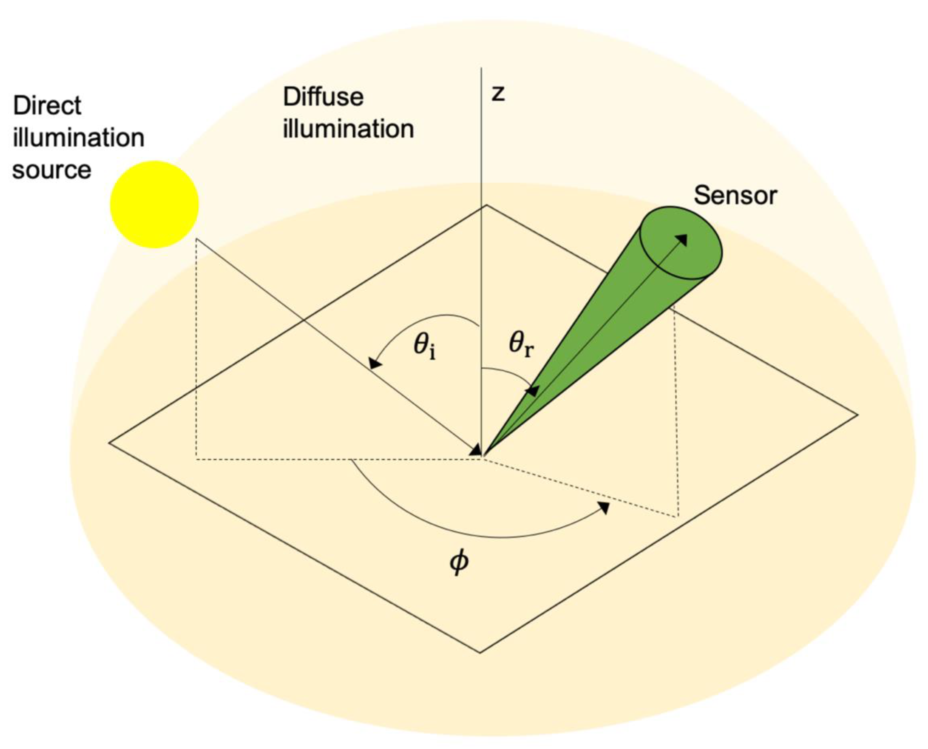
5.1. Definition of Reflectance, BRDF, and Albedo

Standardized nomenclature for reflectance quantities were defined in terms of incident and reflected beam geometry by Nicodemus et al. [255] and later adapted for common optical remote sensing measurement configurations [256,257,258,259]. Here we briefly review key definitions of reflectance quantities, following Schaepman-Strub et al. [259]. Spectral radiance, $L$, is the radiant flux in a beam per unit wavelength and per unit area and solid angle of that beam, with SI units [W m⁻² sr⁻¹ nm⁻¹]. Reflectance is the ratio of exitent radiant flux density (radiant exitance, $M$) [W m⁻²] to incident radiant flux density (irradiance, $E$) [W m⁻²], where both the incident and exitent radiance are integrated across the beam geometry [sr] and radiant spectrum [nm] [259]. For passive optical remote sensing measurements, the incident beam geometry is hemispherical and is composed of both direct-beam and diffuse solar radiation (Figure 8). The exitent (reflected) beam geometry is conical, defined by the sensor instantaneous field of view (IFOV), and is composed of both direct-beam and diffuse reflected solar radiation, corresponding to the hemispherical-conical reflectance function (HCRF) described by Schaepman-Strub et al. [259].

The bidirectional reflectance distribution function BRDF [sr⁻¹] describes the scattering of an infinitesimal beam of incident light from one direction in a hemisphere into another direction, and is defined (omitting spectral dependence) as the ratio of directional reflected radiance $L_{\mathrm{r}}$ [W m⁻² sr⁻¹] to incident irradiance $E_{\mathrm{i}}$ [W m⁻²]:

$$BRDF=\frac{\mathrm{d}{L}_{\mathrm{r}}({\theta }_{\mathrm{i}},{\varphi }_{\mathrm{i}},{\theta }_{\mathrm{r}},{\varphi }_{\mathrm{r}})}{\mathrm{d}{E}_{\mathrm{i}}\left({\theta }_{\mathrm{i}},{\varphi }_{\mathrm{i}}\right)}$$

(6)

where ${\theta }_{\mathrm{i}}$ and ${\theta }_{\mathrm{r}}$ are the incident and reflected viewing angle, respectively, and ${\varphi }_{\mathrm{i}}$ and ${\varphi }_{\mathrm{r}}$ are the incident and reflected azimuth angles, respectively. As a ratio of infinitesimal quantities, the BRDF is a theoretical construct that cannot be directly measured but describes the intrinsic reflectance properties of a surface from which measurable quantities can be derived [259]. For example, integration of the BRDF across ${\theta }_{\mathrm{r}}\left(0\to \mathsf{\pi }/2\right)$ and ${\varphi }_{\mathrm{r}}\left(0\to 2\pi \right)$ yields bihemispherical reflectance, or what is commonly called albedo.

Viewing geometry is important because every natural earth surface is an anisotropic reflector. For example, snow and ice are strongly forward scattering at the particle scale, especially at visible wavelengths, but ice surfaces can be strongly backward scattering due to surface roughness [260]. Consequently, an estimate of the BRDF is required to convert multi-angular reflectance measured by satellite remote sensing instruments to albedo. To achieve this, the BRDF for each satellite ground footprint is estimated (not measured) from repeat multi-angular reflectance measurements collected over time and, therefore, under varying illumination conditions [251] or collected instantaneously by spaceborne multi-angular instruments [261]. A complete technical discussion of the BRDF is available from Schaepman-Strub et al. [259].

5.2. Optical Reflectance and Albedo Sensors and Datasets

Spatially- and temporally-consistent repeat measurements of surface reflectance, and estimates of BRDF and albedo for the Greenland Ice Sheet are provided by satellite-borne imaging spectrometers, including the NASA Moderate Resolution Imaging Spectroradiometer (MODIS), the NASA Multi-angle Imaging SpectroRadiometer (MISR), and the National Oceanic and Atmospheric Administration’s Advanced Very High Resolution Radiometers (AVHRR) (

Table 2. Summary of optical and near-infrared remote sensing platforms, instruments, temporal coverage, observed wavelengths, and managing agencies.

Platform *	Instrument Ŧ	Temporal Coverage	Observed Wavelength	Agency §,Ɣ
Nimbus 1-4	AVCS/IDCS	1964–1980	(1 band) 0.45–0.65 μm	NASA
Landsat 1-5	MSS	1972–2013	(4 bands): 0.55–0.955 μm	NASA/USGS
GOES 1-15	VISSR	1975–present	(5 bands): 0.62–12 μm	NASA/NOAA
Seasat	VIRR	1978 (110 days)	(2 bands): 0.49-0.94, 10.5–12.5 μm	NASA
TIROS-N, NOAA-6,8,10	AVHRR	1978–2001	(4 bands): 0.63–11 μm	NOAA/NASA
NOAA-7,9,11-14	AVHRR/2	1981–present	(5 bands): 0.63–12 μm	NOAA
Landsat 4-5	TM	1982–2013	(7 bands): 0.485–11.45 μm	NASA
Spot 1-3	HRV	1985–2009	(3 bands): 0.55–0.83 μm	CNES/Spot Image
ERS-1	ATSR	1991–2000	(4 bands): 1.6–12.0 μm	ESA
JERS-1	OPS	1992–1998	(8 bands): 0.52–2.40 μm	JAXA
ERS-2	ATSR-2	1995–2011	(7 bands): 0.55–12.0 μm	ESA
ADEOS	POLDER	1996–1997	(9 bands): 0.44–0.91 μm	CNES
ADEOS	AVNIR	1996–1997	(4 bands): 0.42–0.89 μm	JAXA
Spot 4	HRVIR	1998–2013	(4 bands): 0.55–1.63 μm	CNES/Spot Image
NOAA-15-19, MetOp A-C	AVHRR/3	1998–present	(6 bands): 0.63–12.0 μm	NOAA/EMSO
Landsat 7	ETM+	1999–present	(7 bands): 0.49–11.45 μm	NASA/USGS
Ikonos-2	OSA	1999–present	(4 bands): 0.45–0.86 μm	DigitalGlobe
EO-1	Hyperion	2000–2017	(242 channels): 0.35–2.5 μm	NASA/USGS
EO-1	ALI	2000–2017	(9 bands): 0.44–2.2 μm	NASA/USGS
Aqua, Terra	MODIS	2000–present	(36 bands): 0.412–14.2 μm	NASA
Terra	MISR	2000–present	(4 bands) ¥: 0.446–0.867 μm	NASA
Terra	ASTER	2000–present	(14 bands): 0.56–11.3 μm	NASA
QuickBird-2	BGIS2000	2001–2015	(4 bands): 0.45–0.9 μm	DigitalGlobe
ADEOS-2	POLDER	2002–2003	(9 bands): 0.44–0.91 μm	CNES
ADEOS-2	GLI	2002–2003	(36 bands): 0.38–11.95 μm	JAXA
EnviSat	MERIS	2002–2012	(15 bands): 0.39–1.04 μm	ESA
EnviSat	AATSR	2002–2012	(7 bands): 0.55–12.0 μm	ESA
Spot 5	HRG/HRS	2002–2015	(4 bands): 0.55–1.63 μm	CNES/Spot Image
ALOS	AVNIR-2	2006–2011	(4 bands): 0.46–0.82 μm	JAXA
WorldView-1	WV60	2007–present	(1 band): 0.45–0.90 μm	DigitalGlobe
GeoEye-1	GIS	2008–present	(4 bands): 0.45–9.2 μm	DigitalGlobe
WorldView-2	WV110	2009–present	(8 bands): 0.40–1.04 μm	DigitalGlobe
Suomi NPP	VIIRS	2011–present	(22 bands): 0.41–12.01 μm	NASA
Spot 6	NAOMI	2012–present	(4 bands): 0.48–0.82 μm	CNES/Spot Image
Landsat 8	OLI	2013–present	(9 bands): 0.44–2.19 μm	USGS/NASA
Landsat 8	TIRS	2013–present	(2 bands): 10.9, 12 μm	USGS/NASA
Spot 7	NAOMI	2014–present	(4 bands): 0.48–0.82 μm	CNES/Spot Image
WorldView-3	WV-3 Imager	2014–present	(29 bands): 0.40–2.365 μm	DigitalGlobe
Sentinel-2A/B	MSI	2015–present	(13 bands): 0.444–2.202 μm	ESA
GeoEye-2	SpaceViewTM 110	2016–present	(4 bands): 0.45–9.2 μm	DigitalGlobe
Sentinel-3A/B	OLCI	2016–present	(21 bands): 0.40–1.02 μm	ESA
GCOM-C1	SGLI	2017–present	(19 bands): 0.38–12.0 μm	JAXA

*,^Ŧ,^§ See Abbreviations at end of article for expanded acronyms. ^Ɣ Managing agencies are identified by the WMO OSCAR database (Table A1) and may not reflect joint collaborations. ^¥ Observed fore and aft of nadir @ 26°, 45°, 60°, 70.5°.

) [261,262,263,264]. Other notable spaceborne sensors providing surface reflectance that have been used to study the GrIS ablation zone include the Enhanced Thematic Mapper Plus (ETM+) onboard Landsat 7, the Operational Land Imager (OLI) onboard Landsat 8, the ASTER onboard Terra, the High Resolution imagers onboard the Satellite Pour l’Observation de la Terre (SPOT 1-7), the Global Land Imager (GLI) onboard the Advanced Earth Observing Satellite II (ADEOS-2), the Multispectral Imager (MSI) onboard Sentinel-2, and the Ocean Colour and Land Instrument (OLCI) onboard Sentinel-3A/B (Table 2) [265,266,267,268,269,270,271].

The NOAA Extended AVHRR Polar Pathfinder (App-X) product provides surface broadband all-sky albedo and a suite of surface radiative flux and cloud property variables on a 25 km equal area grid twice-daily for the period 1982 to present for the Arctic and Antarctic regions [272]. The AVHRR App-X product provides a continuous record of GrIS surface albedo and an important climatological dataset [253]. An early demonstration of AVHRR surface albedo retrieval revealed a region of anomalously dark ice in the southwestern GrIS ablation zone later termed the “Dark Zone” (Section 5.3) [273]. Although rigorous quality control procedures are applied during dataset production [49], its utility for investigations of GrIS ablation zone albedo may be limited by geolocation errors, four-channel spectral resolution, and inter-mission biases [274,275]. Spatial and spectral resolution are both improved with MODIS, which measures surface reflectance in 30 narrow spectral bands at 250–500 m spatial resolution.

Higher spectral and/or spatial resolution reflectance products are provided by Landsat, MISR, SPOT, Sentinel, and other spaceborne spectrometers (Table 2). Various albedo estimations exist for most sensors [276]. Many rely on the MODIS BRDF or empirical conversions from narrowband reflectance to broadband albedo, and for others (e.g., MISR), a unique BRDF and physically-based albedo estimation exists [261,277]. Most studies of the GrIS albedo have used MODIS albedo owing to the development of operational, publicly available data products spanning nearly two decades. Two MODIS albedo products are currently available: (1) the 500-m Terra/Aqua MODIS 8-day BRDF/Albedo product (MCD43) and, (2) the 500-m Terra daily snow/ice cover and BRDF/Albedo product (MOD10A) [251,263,278]. The MCD43 algorithm uses cloud-free, multi-date, atmospherically corrected input data from combined Terra (MOD09) and Aqua (MYD09) multi-angular surface reflectance retrievals to estimate a unique BRDF for each MODIS pixel in the seven MODIS ‘Land’ bands (1–7) every eight days. Albedo is calculated using this BRDF estimation for each of bands 1–7, and also for three broadbands (0.4–0.7, 0.7–3.0, and 0.4–3.0 um) [251,278].

The MOD10A algorithm is a daily product that uses the discrete-ordinate radiative transfer (DISORT) model to convert MOD09 daily surface reflectance to spectral albedo [279]. The daily frequency of the MOD10A product makes it particularly useful for studies of the GrIS ablation zone, where day-to-day albedo variability is substantial [26,280]. Both the MCD43 and MOD10A retrieval algorithms require cloud-free images, as identified by the MOD35 cloud mask. For the MCD43 product, data gaps within the 16-day period window may result in under-sampling of the BRDF, requiring the use of a backup BRDF algorithm. Albedo values estimated with the backup algorithm are generally considered less reliable, and quality flags are provided to distinguish between them [281].

The accuracy of MODIS albedo over the GrIS has been evaluated by comparison with surface-based measurements of albedo at Greenland Climate Network (GC-Net) automatic weather stations (AWS) [282]. The MCD43 product has an average root mean squared difference (RMSD) of ±0.07 and mean bias +0.022 relative to AWS albedo, which has ±0.035 RMSD uncertainty relative to precision pyranometer measurements [278,283]. The MCD43 RMSD is reduced to ±0.04 when only the highest-quality flagged values are used [283]. MODIS albedo accuracy is reduced at a high solar zenith angle (SZA) [263,283]. For example, Wang and Zender [284] found a large MCD43 albedo bias relative to GC-Net AWS albedo in the dry-snow zone for SZA > 55°. However, these biases are mostly eliminated if only the highest-quality flagged values are used as recommended [281]. In general, the MODIS albedo products are not recommended for comparison with surface measurements for SZA > 70° [281,283].

Relative to three AWS stations in the southwestern GrIS ablation zone, the MOD10A albedo is lower by up to 0.10 and by 0.06 on average during July for the period 2009–2016 [280]. The low bias is attributed to the inadequate sampling of surface heterogeneity by the AWS, which are preferentially located on flat areas of bare ice rather than areas of lower albedo, such as meltwater channels or crevasses that influence the satellite albedo [280]. Using one day of high quality in situ spectral albedo measurements (N = 232) collected within two MODIS satellite pixel ground footprints in the southwest GrIS ablation zone, Moustafa et al. [285] showed that the MODIS Collection V006 daily blue-sky albedo was accurate to within −0.04 to +0.07 for the homogeneous surface of one pixel and was biased low by −0.04 to −0.07 for the heterogeneous surface of the second pixel. As in Ryan et al. [280], the low bias was attributed to under sampling of dark meltwater channels and shadowed crevasses. In addition to spatial heterogeneity, comparisons between satellite albedo and surface measurements are complicated by factors including sensor spectral sensitivity and whether hemispherical or angular reflectance is measured [281,283]. Owing to these varied processes, ground validation of satellite albedo products for the GrIS ablation zone is challenging, and satellite retrieval uncertainty is enhanced relative to the interior snow-covered accumulation-zone surface, especially at sub-pixel scale [280,285,286].

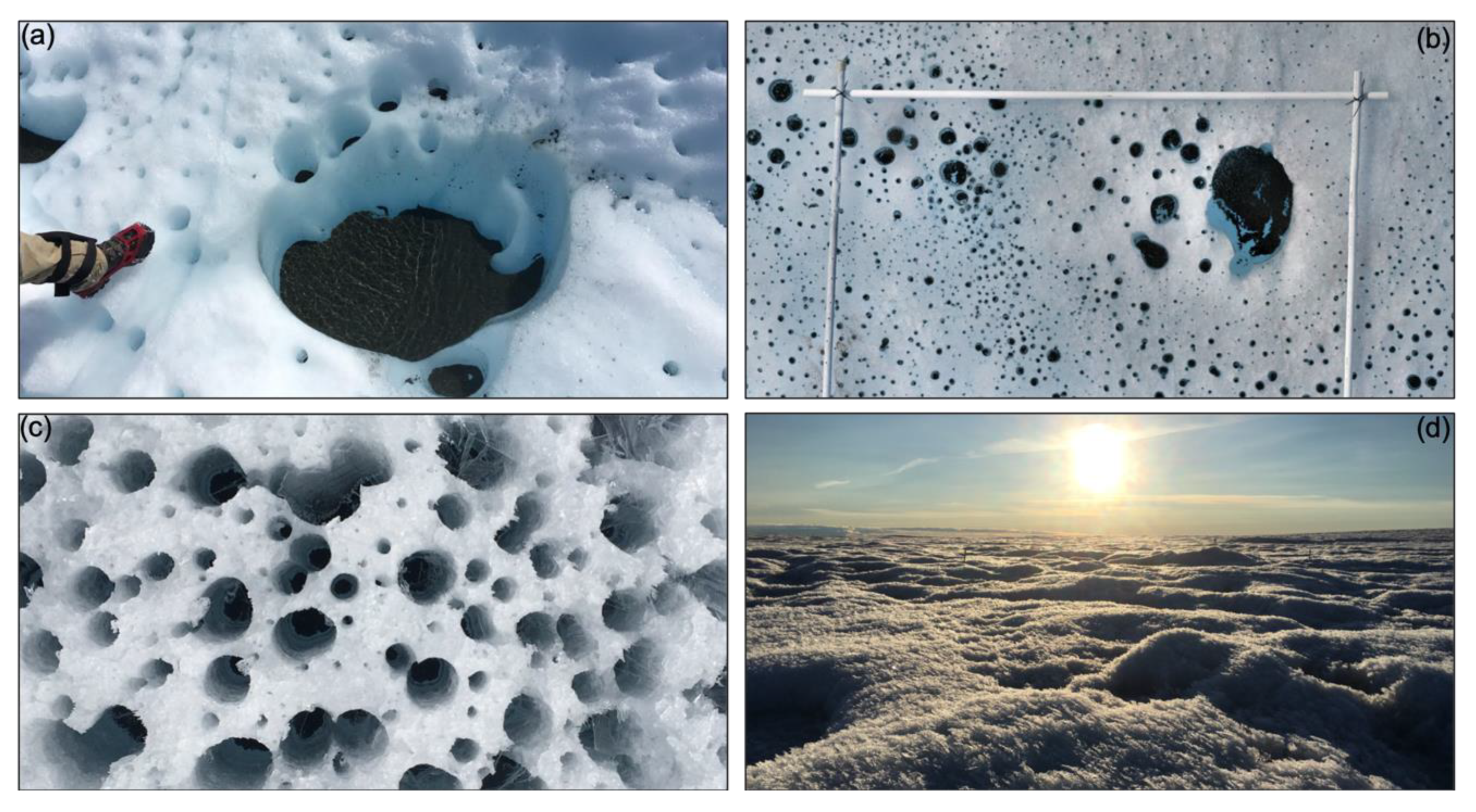
5.3. Dark Ice in the Ablation Zone: Albedo Trends and Drivers

Satellite albedo retrievals provide an important marker of the changing ice surface. The MOD43 data suggest the GrIS area-averaged albedo for June, July, and August (JJA) decreased by −0.044 between 2000–2012 [278]. The JJA albedo anomaly during the record 2012 pan-GrIS melt event [287] was more than two standard deviations below the period mean. The most negative albedo trends are observed for the southern and western ice sheet ablation area where July albedo trends are −0.12 to −0.24 per decade, attributed to both reduced seasonal snow cover duration and increased bare ice exposure during this period [29,30,278]. The MOD10A product indicates a similar JJA albedo trend of −0.083 averaged over the GrIS ablation zone for the period 2000–2010 [30] and −0.078 for the period 2000–2013 [288]. Although MOD10A reflectance data suggest a modest brightening of the ablation zone since 2013 that likely reflects anomalously cold and snowier spring and summer conditions during this period [26,51], there is strong potential for melt-albedo feedbacks to accelerate negative $SMB$ in the coming years [30,32].

For the ablation zone, spatial and temporal albedo variability is driven foremost by the seasonal snowline position and its control on bare ice exposure (Figure 9) [26]. Where snow is present, snow grain growth is the strongest modifier of surface albedo [252,253]. Bare ice albedo is scale dependent but is principally controlled by air bubble size and shape distribution, shadowing by cracks and crevasses [285,289], and by ice grain metamorphism, surface meltwater presence, and exposure and deposition of mineral and biological light-absorbing impurities (LAI) [51,52,58,253,290,291,292]. The darkening effect of LAI is particularly apparent in satellite images of the GrIS ablation zone that reveal foliated bands of “dark ice” with anomalously low albedo relative to surrounding ice (Figure 10) [52,273,293,294]. The wavy appearance of these foliated bands and their static position indicate their provenance as outcropping ice layers rich in dust deposited during past millennia [52,294,295,296].

The spatial extent of bare ice and albedo variability within the bare ice zone exerts a primary control on ice sheet albedo and surface meltwater production in the ablation zone [26,30]. Shimada et al. [297] used MODIS/Terra surface reflectance to quantify the regional distribution of bare ice and dark ice extent during July for the period 2000–2014. The spatial extent of bare ice ranged from 5–16% of the GrIS surface area, dark ice ranged from 4–10%, and both exhibited a positive trend (4.4% yr⁻¹ for bare ice and 7.6% yr⁻¹ for dark ice) with the greatest expansion in the southwest ablation zone. Bare ice extent was strongly correlated ($r = 0.66$) with air temperature, whereas dark ice extent was weakly correlated with air temperature and was negatively correlated with solar radiation, suggesting that bare ice weathering by solar radiation may reduce dark ice extent and increase surface albedo in the GrIS ablation zone (Figure 11).

Recent work highlights the darkening effect of biological LAI on bare ice albedo, including assemblages of biologically-active dust termed “cryoconite” that melt quasi-cylindrical holes into the ice (Figure 11) [298] and distributed communities of algae and cyanobacteria that inhabit the ice surface [299]. For example, Tedstone et al. [51] applied the bare ice and dark ice detection algorithm from Shimada et al. [297] to MODIS surface reflectance imagery of the southwest ablation zone during June–July–August for the period 2000–2016. In contrast to Shimada et al. [297], they conclude that distributed algae blooms, rather than bare ice weathering and cryoconite hole growth, likely explains dark ice dynamics in their study region, owing to the synchronous and abrupt timing of dark ice exposure across the study area and the progressive rather than episodic increase in dark ice extent from June to August. In general, the deepening of cryoconite holes into the ice surface appears to limit their regional effect on albedo, especially at a low sun angle (Figure 11d), whereas distributed LAI that accumulate on the ice surface are considered stronger agents of bare ice darkening in the GrIS ablation zone [58,300]. Understanding seasonal and interannual relationships between bare ice structure, mineral and biological LAI, and bare ice albedo driven by cryoconite hole deepening and removal, weathering crust growth and decay, rotting and removal of superimposed ice, and variations in ice grain and air bubble geometry remain important areas of research that currently elude confident detection by satellite remote sensing [51,85,297,301,302].

5.4. Current Challenges and Future Opportunities

Contemporary research on GrIS ablation zone surface reflectance and albedo is focused on understanding and diagnosing agents of albedo change [253]. Important questions remaining unresolved include whether observed reductions in GrIS snow albedo are caused by enhanced snow grain metamorphism due to a warming climate [252], or by deposition of LAI such as dust and black carbon from industrial emissions and/or forest fire [292,303]. These questions cannot currently be answered owing to the spectral and radiometric limitations of existing spaceborne optical sensors and inadequate surface validation measurements [280,304]. For example, it is unlikely that the albedo-reducing effect of industrial black carbon emissions on relatively clean accumulation zone snow can be detected from space [305,306]. Similarly, it is unknown if bare ice albedo reduction due to deposition or emergence of inorganic mineral LAI can be distinguished using satellite imagery from albedo reduction due to biological LAI [292,301].

To date, efforts to remotely sense changing bare ice albedo have focused on quasi-physical proxies such as “darkening” in broad spectral bands [51,58]. Hyperspectral reflectance is used to map the albedo-reducing effect of LAI, including snow algae and dust in mountain environments and valley glaciers elsewhere [307,308]. However, ice algae are taxonomically distinct from snow algae [291], and optical methods developed by the snow albedo community need to be adapted to detect ice algae or separate its effect on ice albedo from inorganic impurities or variations in ice grain size and structure [292,301]. At present, no spaceborne hyperspectral imager operates over the polar regions, although several hyperspectral missions are planned for the coming years [309]. Recently, multispectral reflectance imagery from the OLCI onboard Sentinel-3A was used to infer the spatiotemporal distribution of ice algal blooms in the southwest GrIS ablation zone, providing insight into the capability of enhanced spectral resolution for diagnosing albedo change in the polar regions [269]. While this represents an important first step toward bioalbedo detection from space, additional ground validation of cellular optical properties specific to the microbial communities on the GrIS surface is needed to discriminate the individual drivers of bare ice albedo reduction using satellite remote sensing [301,310].

6. Mapping Surface Melt and Glaciological Zones

Mapping of surface zones or facies, such as dry snow, wet snow, and bare ice, was pioneered by Benson [35], and later mapped across the GrIS using both ERS SAR imagery [50] and Seasat-A scatterometer backscatter [311]. In contrast to the climatological facies of Benson [35], the concept of radar glacier zones was introduced to distinguish dynamic zones driven by the seasonal cycle of surface melt onset, surface roughening, and snowline migration, thereby revealing the seasonal extent of the bare ice ablation zone [312,313,314]. Multi-angular optical reflectance, together with derived surface roughness, provides an independent method to map glacier zones on the GrIS with particular relevance to ablation zone studies owing to the unique ability of angular reflectance to detect crevasse fields and the lower limit of superimposed ice [53]. These classification approaches are complemented by an extensive legacy of surface melt detection studies using active microwave backscatter, and thermal and passive microwave brightness temperature, which together provide a comprehensive view of the ablation zone surface and changes in ice sheet melt extent with time [55,315,316,317,318,319].

6.1. Active Microwave Detection of Surface Melt and Glacier Zones

SAR imagers measure radar backscatter (image brightness) at (typically) C-band (5 GHz) and Ku-band (14 GHz) frequencies (

Table 3. Summary of active microwave (synthetic aperture radar and microwave scatterometer) remote sensing platforms, instruments, temporal coverage, observed frequencies, and managing agencies.

Platform *	Instrument Ŧ	Temporal Coverage	Observed Frequency	Agency §
Synthetic Aperture Radar
Seasat	SAR	1978 (110 days)	1.275 GHz (L)	NASA
ERS-1	AMI-SAR	1991–2006	5.3 GHz (C)	ESA
JERS-1	SAR	1992–1998	1.2 GHz (L)	JAXA
ERS-2	AMI-SAR	1995–2011	5.3 GHz (C)	ESA
RADARSAT-1	SAR	1995–2013	5.3 GHz (C)	CSA
EnviSat	ASAR	2002–2012	3.2 (S), 5.3 (C), 13.6 GHz (Ku)	ESA
ALOS	PALSAR	2006–2011	1.2 GHz (L)	JAXA
RADARSAT-2	SAR	2007–present	5.3 GHz (C)	CSA
TerraSAR-X	SAR-X	2007–present	9.6 GHz (X)	DLR/EADS
TanDEM-X	SAR-X	2010–present	9.6 GHz (X)	DLR/EADS
CryoSat-2	SIRAL	2010–present	13.9 GHz (Ku)	ESA
Sentinel-1A	SAR-C	2014–present	5.4 GHz (C)	ESA
ALOS-2	PALSAR-2	2014–present	1.2 GHz (L)	JAXA
Sentinel-1B	SAR-C	2016–present	5.4 GHz (C)	ESA
Scatterometers
Seasat	SASS	1978 (110 days)	14.6 GHz (Ku)	NASA
ERS-1	AMI-SCAT	1991–2006	5.3 GHz (C)	ESA
ERS-2	AMI-SCAT	1995–2011	5.3 GHz (C)	ESA
ADEOS	NSCAT	1996–1997	14.0 GHz (Ku)	JAXA
QuikSCAT	SeaWinds	1999–2009	13.4 GHz (Ku)	NASA
ADEOS-2	SeaWinds	2002–2003	13.4 GHz (Ku)	JAXA/NASA
MetOp A-C	ASCAT	2006–present	5.3 GHz (C)	EOMS/ESA

*,^Ŧ,^§ See Abbreviations at end of article for expanded acronyms. ^Ɣ Managing agencies are identified by the WMO OSCAR database (Table A1) and may not reflect joint collaborations.

). Backscatter strength, or the normalized radar cross-section (σ°), is principally controlled by the complex electrical permittivity of the ice surface and by geometric properties, including ice surface roughness, grain size, incidence angle, and ice thermal and physical structure [50,319]. Variations in σ° associated with these controls are used to map zones of unique snow and ice composition on glacier and ice sheet surfaces [320]. An early demonstration of the method used variations in C-band SAR image brightness to map zones of dry snow, percolation, wet snow, and bare ice, extending the early facies work of Benson [35] into the satellite era [50]. Cold, dry, fine-grained snow in the accumulation zone appears dark in C-band imagery, whereas the percolation zone and wet snow zone appear bright, owing to reflections from refrozen ice lenses in the snow/firn column [316]. The bare ice zone is distinguished from the wet snow zone using differential brightness between winter and summer images and the bright reflections of rough, crevassed surfaces [50,321].

C- and Ku-band wind scatterometers measure σ° at both vertical (VV) and horizontal (HH) polarization and are used to map the timing of melt onset and the seasonal progression of surface melt extent [313,322]. As with SAR, the method exploits the strong reduction in σ° caused by the presence of liquid water at or near the ice surface. Relative to SAR imagers, scatterometers provide σ° at coarse spatial resolution but high temporal resolution, for example, a 25 km grid size twice-daily for the SeaWinds on NASA’s Quick Scatterometer (QuikSCAT) [322]. Resolution enhancement techniques increase the effective resolution to ~8–10 km [323].

Surface melt on the GrIS and peripheral ice caps has been detected by the Seasat-A scatterometer (SASS), the Advanced Microwave Instrument-Scatterometer (AMI-SCAT) on ERS-1/2, and the SeaWinds scatterometer on both NASA’s Quick Scatterometer (QuikSCAT) and ADEOS-2 (Table 3) [311,320,322,324,325,326]. Methods to detect surface melt include single-channel absolute σ° thresholds [324], diurnal σ° variability (relative thresholds) [322], physical and statistical model-based methods [326], and dual-frequency/polarization thresholds that also use the diurnal difference between ascending and descending orbital passes [327]. The diurnal method exploits contrasts in σ° caused by diurnal melt-freeze cycles. The use of relative thresholds reduces errors from sensor drift, cross-mission biases, or step changes in surface properties, such as ice lens formation that affect absolute thresholds [115]. In addition to discrete melt onset, time-integrated σ° reduction is used to infer seasonal melt intensity [324,325,326].

In addition to mapping surface melt onset and extent, seasonal changes in σ° are used to infer the timing and spatial extent of ice layer formation in snow and firn [115,316,328]. Understanding ice layer formation is important because meltwater refreezing increases firn density without reducing mass and raises the effective backscattering surface detected by radar altimeters, leading to errors in radar mass balance estimates (Section 3.1.2). Nghiem et al. [115] developed a field-validated method that relates threshold increases in QuickSCAT HH-polarized σ^o before and after melt seasons to ice layer formation in the GrIS percolation zone. The method also provides a basis for estimating snow accumulation by integrating σ^o reduction following ice layer formation. The method assumes threshold increases in σ^o are caused by enhanced reflections from newly formed ice layers, whereas the gradual attenuation of σ° following ice layer formation is caused by new snow accumulation. Wang et al. [328] applied the method to five years of enhanced-resolution QuickSCAT imagery [329] and found extensive increases in ice layer formation following a short three-day melt event in 2002, highlighting the disproportionate impact of extreme melt events on ice layer formation.

6.2. Passive Microwave and Thermal Radiometry

At thermal and microwave wavelengths (beyond about 3 um) spectral radiance (converted via the Planck function to brightness temperature, $T_{\mathrm{b}}$) is approximately linear with $T_{\mathrm{sfc}}$: $T_{\mathrm{b}}=\epsilon \ast T_{\mathrm{sfc}}$, where $\epsilon$ is the material emissivity [330]. Whereas σ° is dramatically reduced by liquid water in snow, $T_{\mathrm{b}}$ is dramatically increased, forming the basis for surface melt detection threshold algorithms, typically using a threshold value below freezing to indicate melting [315,331,332]. Passive microwave radiometers measure background microwave emission at (primarily) K-band (~19 GHz) and Ka-band (~37 GHz) frequencies and various combinations of VV and HH polarization (

Table 4. Summary of passive microwave remote sensing platforms, instruments, temporal coverage, observed frequencies, and managing agencies.

Platform *	Instrument Ŧ	Temporal Coverage	Observed Frequency	Agency §
Nimbus-5	ESMR	1972–1983	19 GHz	NASA
Nimbus-6	ESMR	1975–1983	37 GHz	NASA
Seasat	SMMR	1978 (110 days)	7, 10, 18, 21, 37	NASA
Nimbus-7	SMMR	1978–1994	7, 10, 19, 37 GHz	NASA/NOAA
DMSP F08,10-15,18	SSM/I	1987–present	19, 22, 37, 86 GHz	DoD/NOAA
DMSP F16-19	SSMIS	1987–present	19, 22, 37, 92 GHz	DoD/NOAA
ERS-1	ATSR	1991–2006	24, 37 GHz	ESA
GFO	WVR	1998–2008	22, 37 GHz	DoD/NASA
ADEOS-2	AMSR	2002–2003	7, 10, 19, 24, 37, 89A, 89B GHz	JAXA/NASA
Aqua	AMSR-E	2002–2011	7, 10, 19, 24, 37, 89 GHz	NASA
ERS-2, EnviSat	MWR	2002–2012	24, 37 GHz	ESA
GCOM-W1	AMSR-2	2012–present	7 (dual), 10, 19, 37, 89 GHz	NASA/JAXA
Sentinel 3A/B	MWR	2016–present	24, 37 GHz	ESA

*,^Ŧ,^§ See Abbreviations at end of article for expanded acronyms. ^Ɣ Managing agencies are identified by the WMO OSCAR database (Table A1) and may not reflect joint collaborations.

). In contrast to the higher spatial resolution (~10 km²) but the lower temporal resolution (weeks to months) of spaceborne active microwave sensors, passive microwave sensors provide $T_{\mathrm{b}}$ twice-daily at ~25–50 km² spatial resolution and complete ice sheet coverage. Melt detection methods using $T_{\mathrm{b}}$ include single-channel thresholds [332,333], dual frequency/polarization combinations (cross polarized gradient ratio XPGR) [315,334], and diurnal amplitude variations (DAV) on ascending and descending passes [335,336]. As with σ°, microwave $T_{\mathrm{b}}$ is strongly modified by liquid meltwater presence at the ice sheet surface but typically does not provide information about the internal snow or firn structure [324,337].

With more than 30 years of continuous data collection, pan-GrIS spatial coverage, and all-weather capability, spaceborne passive microwave radiometers provide a unique insight into the climatic drivers of ice sheet surface mass balance processes, including changes in the location and extent of surface melting (Figure 12) [315,317,318,334,336,338,339]. Data from the Special Sensor Microwave/Imager (SSM/I) suggests the area of active surface melt over the GrIS has approximately doubled since the early 1990s, with a 40,000 km² yr⁻¹ trend during this period [318,336]. Data from the Scanning Multichannel Microwave Radiometer (SMMR, 1978-1987) and SSM/I were used to characterize the effects of the Mt. Pinatubo eruption on GrIS surface melt patterns [340]. Surface melt extent from SSM/I has been correlated with downstream sediment plume concentrations in Greenland fjords driven by ice sheet meltwater discharge [341], to validate surface melt extent calculated from surface energy balance models [342,343], and to quantify extreme events such as the record July 2012 melt event when 98.6% of the GrIS surface was actively melting [287,339].

Thermal radiance (~3–14 μm) is used to map $T_{\mathrm{sfc}}$ and provides an additional method for surface melt detection [345]. Variations in thermal and optical radiance form the basis for mapping “reflectance zones” to characterize melt presence and changes in the thermal structure on glacier surfaces [346]. Whereas σ° and microwave $T_{\mathrm{B}}$ are primarily diagnostic of melt presence, both at or near the surface, thermal radiance is diagnostic of the surface “skin” temperature, and provides little to no information about subsurface temperature, meltwater presence, or snow and firn structure. Consequently, thermal $T_{\mathrm{sfc}}$ is strictly an indicator of surface melt and, together with the higher spatial and radiometric resolution of thermal sensors such as MODIS, provides an independent method for validating active and passive microwave melt presence products [347,348]. When combined with microwave melt presence and remotely sensed albedo, thermal $T_{\mathrm{sfc}}$ may improve the discrimination of surface and subsurface melt areas and diurnal variations in melt-freeze cycles [347]. As with microwave surface melt detection, thermal radiance melt detection has been used to validate modeled surface melt [318,342], and to study the spatiotemporal variation of surface melt extent and duration on the GrIS and its relation to climatic variability [55,238,348,349,350].

The primary spaceborne thermal sensors used to obtain $T_{\mathrm{sfc}}$ are MODIS and AVHRR. The NOAA Extended AVHRR Polar Pathfinder (App-X) product provides $T_{\mathrm{sfc}}$ on a 25 km polar equal-area grid twice-daily for the period 1982 to present [272]. As with the AVHRR albedo product (Section 5.2), there are spectral, radiometric, and inter-mission homogenization issues that limit its utility [351]. The MODIS land surface temperature product (MOD11A1) uses the split-window technique developed for AVHRR to calculate $T_{\mathrm{sfc}}$ from radiance at 10.78 μm and 11.77 μm [352]. The MOD11A1 data are provided on a 1 km grid globally for clear-sky conditions as discriminated by the MOD35 cloud mask. The MOD11A1 product is accurate to ± 1 °C on average over snow and ice surfaces and agrees to within ± 0.5 °C with $T_{\mathrm{sfc}}$ calculated from ASTER and Landsat ETM+ thermal radiance over the GrIS [350]. Surface melt extent from MOD11A1 corresponds closely to surface melt inferred from QuickSCAT using the diurnal σ^o method [347].

The Greenland Ice Surface Temperature (IST) product is an enhanced version of MOD11A1 that provides IST and binary melt absence/presence for the period 2000–2014 on a 1.25 km polar stereographic grid for the GrIS [349,351]. For values of $T_{\mathrm{sfc}}$ near 0 °C, the IST data are −0.5 °C cooler than surface-based $T_{\mathrm{sfc}}$ measurements collected at the Summit Station [353,354]. The bias increases to −5.0 °C for values of $T_{\mathrm{sfc}}$ near −60 °C and increases with SZA, suggesting the bias may be related to reduced accuracy of the MOD35 cloud mask at high SZA. Under-sampling of $T_{\mathrm{sfc}}$ during warm inversions with dense cloud coverage may also introduce bias but this effect has not been systematically evaluated [353,354]. In general, spaceborne thermal $T_{\mathrm{sfc}}$ retrievals are effective for detecting surface melt during clear-sky conditions but are sensitive to the atmospheric aerosol and water vapor profile [351,355]. To overcome cloud-cover data gaps, Välisuo et al. [348] gap-filled the IST product with modeled values of $T_{\mathrm{sfc}}$ from the European Centre for Medium-Range Weather Forecasts ERA-Interim reanalysis.

6.3. Multi-Angular Reflectance and Surface Roughness

The Multi-angle Imaging SpectroRadiometer (MISR) measures coincident-in-time bi-directional radiance in four spectral bands between 450–850 nm at 0° (nadir), 26.1°, 45.6°, 60.0°, and 70.5° fore and aft of nadir. Reflectance is provided on a 275 m grid and nine-day global coverage to ±83° (Table 2) [260]. The normalized difference angular index (NDAI) was developed to estimate ice surface roughness from MISR angular reflectance [260]. The method uses an empirical relationship between MISR red band reflectance at 60^o fore and aft of nadir and ATM lidar-derived surface roughness to develop spatially-continuous maps of surface roughness over ice sheets and sea ice [356]. The MISR NDAI and near-infrared albedo (Section 5.2) were used to map unique signatures of surface glaciological features in the western GrIS ablation zone, including crevasse fields, wet snow, and bare glacier ice [53]. With this approach, MISR angular reflectance appears to provide a unique method for detecting the superimposed ice zone and may improve the identification of changes in crevasse field roughness relative to SAR and optical sensors [53,260].

Surface roughness controls ice–atmosphere interactions via the aerodynamic roughness length and the net vapor flux, an understudied component of the GrIS $SMB$ [60,82,357]. The MISR surface roughness product [356] was used to define the aerodynamic roughness length of the BMF13 vapor flux model to improve the spatial realism of net vapor flux in the ablation zone where roughness is highly variable [357]. The average annual modeled vapor flux was 14.6 ± 3.6 Gt yr⁻¹, or 6 ± 2% of annual $SMB$ for the period 2003–2014. The average annual difference between modeled vapor flux with and without MISR roughness was 30 ± 15%. In addition to angular reflectance, surface roughness has been quantified from ICESat and ATM laser altimetry waveforms [173,358,359]. The forthcoming ICESat-2 laser altimeter may provide additional capability for measuring surface roughness on the GrIS, for example using the multi-sensor lidar-angular reflectance approach of Nolin and Mar [356] and Nolin et al. [260], which may also be useful for radar altimetry waveform interpretation of the leading edge of the beam footprint [93].

6.4. Future Opportunities for Mapping the Changing GrIS Ablation Zone Surface

The GrIS surface is undergoing rapid change, driven by increased surface meltwater production in the ablation zone. Spaceborne SAR imagers, wind scatterometers, and passive microwave, thermal, and angular radiometers are used to map and monitor diagnostic features of change on the ablation zone surface, including surface melt presence and extent, subsurface ice layer formation, ice surface temperature, and ice surface roughness. These characteristic features are used to define and map the dry snow zone, wet snow zone, percolation zone, superimposed ice zone, and the bare ice zone. Mapping of supraglacial hydrologic features, including meltwater lakes, rivers, and moulins stands out as an additional research priority c.f. [68], in particular, their expansion and inland migration toward sensitive (e.g., high elevation) areas of the ice sheet [56,360,361]. Other diagnostic markers of change detectable in satellite imagery include the end of summer snowline position (Figure 9) [26], the lower limit of superimposed ice [53], and the lower limit of the slush zone [293]. Multi-sensor methods, for example, optical imagery combined with SAR imagery or scatterometry, shows promise for detecting dynamic regions characterized by changing snow, firn, and ice surface types, including supraglacial lakes and slush fields obscured by snow or clouds, and may reduce detection bias caused by cloud cover [362,363,364].

7. Conclusions

For over forty years, earth-observing satellites sensitive to visible, infrared, and microwave electromagnetic radiation, together with gravimetry, have documented the patterns of change on the GrIS ablation zone surface. Satellite remote sensing data show an ablation zone expanded in size, its albedo and surface elevation lower in response to enhanced melting and ice discharge, and an ice sheet transition from steady state to negative mass balance that now represents the largest land ice contributor to global sea level rise. Already, some 78–85% of the total liquid runoff produced from surface melting is generated in the bare ice ablation zone, despite it covering ~22% of the ice sheet’s total surface area, up from ~15% in the early 1960s [20,30,33,34,35]. Although often conceptualized as a uniform surface of solid ice, the ablation zone is a dynamic region with widely varying electromagnetic properties controlled by diverse physical, biological, and hydrologic processes. Future progress in remote sensing the ablation zone will likely benefit most from methods that directly address this complexity, for example, using multi-sensor, multi-wavelength, and cross-platform datasets. Examples include fusing radar and laser altimetry with optical stereophotogrammetry to discriminate and diagnose causes of surface elevation change [174], or fusing radar and laser backscatter with optical imagery to discriminate snow, ice, liquid water, and refrozen meltwater in sensitive areas near the equilibrium line altitude [362,363]. Other areas of opportunity recommended for future research include spaceborne detection of subsurface refrozen meltwater and its effects on radar backscatter, which requires additional in-situ validation [115,116], the partitioning of ablation zone thinning into ice-dynamic and surface mass balance components [97], cross-validation of ice surface elevation change from altimetry with modeled surface mass balance [89] and modeled ice dynamic motion [189], spaceborne diagnosis of changing bare ice albedo [269] and grain size [191], and monitoring the inland migration of snowlines, surface melt extent, and surface hydrologic features including lakes, streams, and moulins [26,56].

References

1. Van den Broeke, M.R.; Enderlin, E.M.; Howat, I.M.; Kuipers Munneke, P.; Noël, B.P.Y.; van de Berg, W.J.; van Meijgaard, E.; Wouters, B. On the recent contribution of the Greenland ice sheet to sea level change. Cryosphere 2016, 10, 1933–1946. [Google Scholar] [CrossRef] [Green Version]
2. Hanna, E.; Huybrechts, P.; Steffen, K.; Cappelen, J.; Huff, R.; Shuman, C.; Irvine-Fynn, T.; Wise, S.; Griffiths, M. Increased Runoff from Melt from the Greenland Ice Sheet: A Response to Global Warming. J. Clim. 2008, 21, 331–341. [Google Scholar] [CrossRef] [Green Version]
3. Vizcaíno, M.; Mikolajewicz, U.; Gröger, M.; Maier-Reimer, E.; Schurgers, G.; Winguth, A.M.E. Long-term ice sheet–climate interactions under anthropogenic greenhouse forcing simulated with a complex Earth System Model. Clim. Dyn. 2008, 31, 665–690. [Google Scholar] [CrossRef]
4. Ettema, J.; van den Broeke, M.R.; van Meijgaard, E.; van de Berg, W.J.; Bamber, J.L.; Box, J.E.; Bales, R.C. Higher surface mass balance of the Greenland ice sheet revealed by high-resolution climate modeling. Geophys. Res. Lett. 2009, 36, L12501. [Google Scholar] [CrossRef]
5. Vizcaíno, M.; Lipscomb, W.H.; Sacks, W.J.; van Angelen, J.H.; Wouters, B.; van den Broeke, M.R. Greenland Surface Mass Balance as Simulated by the Community Earth System Model. Part I: Model Evaluation and 1850–2005 Results. J. Clim. 2013, 26, 7793–7812. [Google Scholar] [CrossRef]
6. Vizcaíno, M.; Lipscomb, W.H.; Sacks, W.J.; van den Broeke, M. Greenland Surface Mass Balance as Simulated by the Community Earth System Model. Part II: Twenty-First-Century Changes. J. Clim. 2013, 27, 215–226. [Google Scholar] [CrossRef]
7. Vizcaíno, M.; Mikolajewicz, U.; Ziemen, F.; Rodehacke, C.B.; Greve, R.; van den Broeke, M.R. Coupled simulations of Greenland ice sheet and climate change up to AD 2300. Geophys. Res. Lett. 2015, 42, 3927–3935. [Google Scholar] [CrossRef]
8. Trusel, L.D.; Das, S.B.; Osman, M.B.; Evans, M.J.; Smith, B.E.; Fettweis, X.; McConnell, J.R.; Noël, B.P.Y.; Broeke, M.R. van den Nonlinear rise in Greenland runoff in response to post-industrial Arctic warming. Nature 2018, 564, 104–108. [Google Scholar] [CrossRef]
9. Pattyn, F.; Ritz, C.; Hanna, E.; Asay-Davis, X.; DeConto, R.; Durand, G.; Favier, L.; Fettweis, X.; Goelzer, H.; Golledge, N.R.; et al. The Greenland and Antarctic ice sheets under 1.5 °C global warming. Nat. Clim. Chang. 2018, 8, 1053–1061. [Google Scholar] [CrossRef]
10. Bamber, J.L.; Westaway, R.M.; Marzeion, B.; Wouters, B. The land ice contribution to sea level during the satellite era. Environ. Res. Lett. 2018, 13, 063008. [Google Scholar] [CrossRef]
11. Hanna, E.; Navarro, F.J.; Pattyn, F.; Domingues, C.M.; Fettweis, X.; Ivins, E.R.; Nicholls, R.J.; Ritz, C.; Smith, B.; Tulaczyk, S.; et al. Ice-sheet mass balance and climate change. Nature 2013, 498, 51–59. [Google Scholar] [CrossRef] [PubMed]
12. Shepherd, A.; Ivins, E.R.; Geruo, A.; Barletta, V.R.; Bentley, M.J.; Bettadpur, S.; Briggs, K.H.; Bromwich, D.H.; Forsberg, R.; Galin, N.; et al. A Reconciled Estimate of Ice-Sheet Mass Balance. Science 2012, 338, 1183–1189. [Google Scholar] [CrossRef] [PubMed] [Green Version]
13. Rignot, E.; Velicogna, I.; van den Broeke, M.R.; Monaghan, A.; Lenaerts, J.T.M. Acceleration of the contribution of the Greenland and Antarctic ice sheets to sea level rise. Geophys. Res. Lett. 2011, 38, L05503. [Google Scholar] [CrossRef]
14. Bevis, M.; Harig, C.; Khan, S.A.; Brown, A.; Simons, F.J.; Willis, M.; Fettweis, X.; van den Broeke, M.R.; Madsen, F.B.; Kendrick, E.; et al. Accelerating changes in ice mass within Greenland, and the ice sheet’s sensitivity to atmospheric forcing. Proc. Natl. Acad. Sci. USA 2019, 116, 1934–1939. [Google Scholar] [CrossRef] [PubMed]
15. Wouters, B.; Bamber, J.L.; van den Broeke, M.R.; Lenaerts, J.T.M.; Sasgen, I. Limits in detecting acceleration of ice sheet mass loss due to climate variability. Nat. Geosci. 2013, 6, 613–616. [Google Scholar] [CrossRef]
16. Kjeldsen, K.K.; Korsgaard, N.J.; Bjørk, A.A.; Khan, S.A.; Box, J.E.; Funder, S.; Larsen, N.K.; Bamber, J.L.; Colgan, W.; van den Broeke, M.; et al. Spatial and temporal distribution of mass loss from the Greenland Ice Sheet since AD 1900. Nature 2015, 528, 396–400. [Google Scholar] [CrossRef] [PubMed]
17. van den Broeke, M.; Bamber, J.; Ettema, J.; Rignot, E.; Schrama, E.; van de Berg, W.J.; van Meijgaard, E.; Velicogna, I.; Wouters, B. Partitioning Recent Greenland Mass Loss. Science 2009, 326, 984–986. [Google Scholar] [CrossRef] [Green Version]
18. Enderlin, E.M.; Howat, I.M.; Jeong, S.; Noh, M.-J.; van Angelen, J.H.; van den Broeke, M.R. An improved mass budget for the Greenland ice sheet. Geophys. Res. Lett. 2014, 41, 866–872. [Google Scholar] [CrossRef] [Green Version]
19. Andersen, M.L.; Stenseng, L.; Skourup, H.; Colgan, W.; Khan, S.A.; Kristensen, S.S.; Andersen, S.B.; Box, J.E.; Ahlstrøm, A.P.; Fettweis, X.; et al. Basin-scale partitioning of Greenland ice sheet mass balance components (2007–2011). Earth Planet. Sci. Lett. 2015, 409, 89–95. [Google Scholar] [CrossRef]
20. Machguth, H.; MacFerrin, M.; van As, D.; Box, J.E.; Charalampidis, C.; Colgan, W.; Fausto, R.S.; Meijer, H.A.J.; Mosley-Thompson, E.; van de Wal, R.S.W. Greenland meltwater storage in firn limited by near-surface ice formation. Nat. Clim. Chang. 2016, 6, 390–393. [Google Scholar] [CrossRef] [Green Version]
21. Lenaerts, J.T.M.; Medley, B.; van den Broeke, M.R.; Wouters, B. Observing and Modeling Ice Sheet Surface Mass Balance. Rev. Geophys. 2019, 57, 376–420. [Google Scholar] [CrossRef] [PubMed]
22. Fettweis, X.; Box, J.E.; Agosta, C.; Amory, C.; Kittel, C.; Lang, C.; van As, D.; Machguth, H.; Gallée, H. Reconstructions of the 1900–2015 Greenland ice sheet surface mass balance using the regional climate MAR model. Cryosphere 2017, 11, 1015–1033. [Google Scholar] [CrossRef]
23. Van Angelen, J.H.; van den Broeke, M.R.; Wouters, B.; Lenaerts, J.T.M. Contemporary (1960–2012) Evolution of the Climate and Surface Mass Balance of the Greenland Ice Sheet. Surv. Geophys. 2014, 35, 1155–1174. [Google Scholar] [CrossRef]
24. Hanna, E.; Cropper, T.E.; Hall, R.J.; Cappelen, J. Greenland Blocking Index 1851–2015: A regional climate change signal. Int. J. Climatol. 2016, 36, 4847–4861. [Google Scholar] [CrossRef]
25. Fettweis, X.; Hanna, E.; Lang, C.; Belleflamme, A.; Erpicum, M.; Gallée, H. Brief communication: Important role of the mid-tropospheric atmospheric circulation in the recent surface melt increase over the Greenland ice sheet. Cryosphere 2013, 7, 241–248. [Google Scholar] [CrossRef]
26. Ryan, J.C.; Smith, L.C.; van As, D.; Cooley, S.W.; Cooper, M.G.; Pitcher, L.H.; Hubbard, A. Greenland Ice Sheet surface melt amplified by snowline migration and bare ice exposure. Sci. Adv. 2019, 5, eaav3738. [Google Scholar] [CrossRef] [Green Version]
27. Hofer, S.; Tedstone, A.J.; Fettweis, X.; Bamber, J.L. Decreasing cloud cover drives the recent mass loss on the Greenland Ice Sheet. Sci. Adv. 2017, 3, e1700584. [Google Scholar] [CrossRef]
28. Lim, Y.-K.; Schubert, S.D.; Nowicki, S.M.J.; Lee, J.N.; Molod, A.M.; Cullather, R.I.; Zhao, B.; Velicogna, I. Atmospheric summer teleconnections and Greenland Ice Sheet surface mass variations: Insights from MERRA-2. Environ. Res. Lett. 2016, 11, 024002. [Google Scholar] [CrossRef]
29. Tedesco, M.; Fettweis, X.; van den Broeke, M.R.; van de Wal, R.S.W.; Smeets, C.J.P.P.; van de Berg, W.J.; Serreze, M.C.; Box, J.E. The role of albedo and accumulation in the 2010 melting record in Greenland. Environ. Res. Lett. 2011, 6, 014005. [Google Scholar] [CrossRef]
30. Box, J.E.; Fettweis, X.; Stroeve, J.C.; Tedesco, M.; Hall, D.K.; Steffen, K. Greenland ice sheet albedo feedback: Thermodynamics and atmospheric drivers. Cryosphere 2012, 6, 821–839. [Google Scholar] [CrossRef]
31. Fürst, J.J.; Goelzer, H.; Huybrechts, P. Ice-dynamic projections of the Greenland ice sheet in response to atmospheric and oceanic warming. Cryosphere 2015, 9, 1039–1062. [Google Scholar] [CrossRef] [Green Version]
32. Franco, B.; Fettweis, X.; Erpicum, M. Future projections of the Greenland ice sheet energy balance driving the surface melt. Cryosphere 2013, 7, 1–18. [Google Scholar] [CrossRef] [Green Version]
33. Steger, C.R.; Reijmer, C.H.; van den Broeke, M.R. The modelled liquid water balance of the Greenland Ice Sheet. Cryosphere 2017, 11, 2507–2526. [Google Scholar] [CrossRef] [Green Version]
34. Bader, H. The Greenland Ice Sheet; Cold Regions Research and Engineering Lab: Hanover, NH, USA, 1961; pp. 1–17. [Google Scholar]
35. Benson, C.S. Stratigraphic Studies in the Snow and Firn of the Greenland Ice Sheet; Cold Regions Research and Engineering Lab: Hanover, NH, USA, 1962; pp. 13–37. [Google Scholar]
36. Pritchard, H.D.; Luthcke, S.B.; Fleming, A.H. Understanding ice-sheet mass balance: Progress in satellite altimetry and gravimetry. J. Glaciol. 2011, 56, 1151–1161. [Google Scholar] [CrossRef]
37. Brooks, R.L.; Campbell, W.J.; Ramseier, R.O.; Stanley, H.R.; Zwally, H.J. Ice sheet topography by satellite altimetry. Nature 1978, 274, 539–543. [Google Scholar] [CrossRef]
38. Sørensen, L.S.; Simonsen, S.B.; Forsberg, R.; Khvorostovsky, K.; Meister, R.; Engdahl, M.E. 25 years of elevation changes of the Greenland Ice Sheet from ERS, Envisat, and CryoSat-2 radar altimetry. Earth Planet. Sci. Lett. 2018, 495, 234–241. [Google Scholar] [CrossRef]
39. Brenner, A.C.; DiMarzio, J.P.; Zwally, H.J. Precision and Accuracy of Satellite Radar and Laser Altimeter Data Over the Continental Ice Sheets. IEEE Trans. Geosci. Remote Sens. 2007, 45, 321–331. [Google Scholar] [CrossRef]
40. Abdalati, W.; Zwally, H.J.; Bindschadler, R.; Csatho, B.; Farrell, S.L.; Fricker, H.A.; Harding, D.; Kwok, R.; Lefsky, M.; Markus, T.; et al. The ICESat-2 Laser Altimetry Mission. Proc. IEEE 2010, 98, 735–751. [Google Scholar] [CrossRef]
41. Drinkwater, M.R.; Francis, R.; Ratier, G.; Wingham, D.J. The European Space Agency’s Earth Explorer Mission CryoSat: Measuring variability in the cryosphere. Ann. Glaciol. 2004, 39, 313–320. [Google Scholar] [CrossRef]
42. Flechtner, F.; Neumayer, K.-H.; Dahle, C.; Dobslaw, H.; Fagiolini, E.; Raimondo, J.-C.; Güntner, A. What can be Expected from the GRACE-FO Laser Ranging Interferometer for Earth Science Applications? In Remote Sensing and Water Resources; Cazenave, A., Champollion, N., Benveniste, J., Chen, J., Eds.; Space Sciences Series of ISSI; Springer International Publishing: Cham, Switzerland, 2016; pp. 263–280. ISBN 978-3-319-32449-4. [Google Scholar]
43. Turyshev, S.G.; Sazhin, M.V.; Toth, V.T. General relativistic laser interferometric observables of the GRACE-Follow-On mission. Phys. Rev. D 2014, 89, 105029. [Google Scholar] [CrossRef]
44. Bjørk, A.A.; Kjær, K.H.; Korsgaard, N.J.; Khan, S.A.; Kjeldsen, K.K.; Andresen, C.S.; Box, J.E.; Larsen, N.K.; Funder, S. An aerial view of 80 years of climate-related glacier fluctuations in southeast Greenland. Nat. Geosci. 2012, 5, 427–432. [Google Scholar] [CrossRef] [Green Version]
45. Gallaher, D.; Campbell, G.G.; Meier, W.; Moses, J.; Wingo, D. The process of bringing dark data to light: The rescue of the early Nimbus satellite data. GeoResJ 2015, 6, 124–134. [Google Scholar] [CrossRef] [Green Version]
46. Bindschadler, R. Monitoring ice sheet behavior from space. Rev. Geophys. 1998, 36, 79–104. [Google Scholar] [CrossRef] [Green Version]
47. Freden, S.C.M. Significant Results Obtained from the Earth Resources Technology Satellite-1. Volume 1: Technical presentations, sections A and B. In Proceedings of the Symposium on Significant Results Obtained from the Earth Resources Technology Satellite-1, New Carrollton, MD, USA, 5–9 March 1973. [Google Scholar]
48. He, T.; Liang, S.; Yu, Y.; Wang, D.; Gao, F.; Liu, Q. Greenland surface albedo changes in July 1981–2012 from satellite observations. Environ. Res. Lett. 2013, 8, 044043. [Google Scholar] [CrossRef]
49. Key, J.; Wang, X.; Liu, Y.; Dworak, R.; Letterly, A. The AVHRR Polar Pathfinder Climate Data Records. Remote Sens. 2016, 8, 167. [Google Scholar] [CrossRef]
50. Fahnestock, M.; Bindschadler, R.; Kwok, R.; Jezek, K. Greenland Ice Sheet Surface Properties and Ice Dynamics from ERS-1 SAR Imagery. Science 1993, 262, 1530–1534. [Google Scholar] [CrossRef]
51. Tedstone, A.J.; Bamber, J.L.; Cook, J.M.; Williamson, C.J.; Fettweis, X.; Hodson, A.J.; Tranter, M. Dark ice dynamics of the south-west Greenland Ice Sheet. Cryosphere 2017, 11, 2491–2506. [Google Scholar] [CrossRef] [Green Version]
52. Wientjes, I.G.M.; Oerlemans, J. An explanation for the dark region in the western melt zone of the Greenland ice sheet. Cryosphere 2010, 4, 261–268. [Google Scholar] [CrossRef] [Green Version]
53. Nolin, A.W.; Payne, M.C. Classification of glacier zones in western Greenland using albedo and surface roughness from the Multi-angle Imaging SpectroRadiometer (MISR). Remote Sens. Environ. 2007, 107, 264–275. [Google Scholar] [CrossRef]
54. Yang, K.; Smith, L.C. Supraglacial Streams on the Greenland Ice Sheet Delineated From Combined Spectral-Shape Information in High-Resolution Satellite Imagery. IEEE Geosci. Remote Sens. Lett. 2013, 10, 801–805. [Google Scholar] [CrossRef]
55. Hall, D.K.; Williams, R.S.; Casey, K.A.; DiGirolamo, N.E.; Wan, Z. Satellite-derived, melt-season surface temperature of the Greenland Ice Sheet (2000–2005) and its relationship to mass balance. Geophys. Res. Lett. 2006, 33, L11501. [Google Scholar] [CrossRef]
56. Gledhill, L.A.; Williamson, A.G. Inland advance of supraglacial lakes in north-west Greenland under recent climatic warming. Ann. Glaciol. 2018, 59, 66–82. [Google Scholar] [CrossRef]
57. Legleiter, C.J.; Tedesco, M.; Smith, L.C.; Behar, A.E.; Overstreet, B.T. Mapping the bathymetry of supraglacial lakes and streams on the Greenland ice sheet using field measurements and high-resolution satellite images. Cryosphere 2014, 8, 215–228. [Google Scholar] [CrossRef] [Green Version]
58. Ryan, J.C.; Hubbard, A.L.; Stibal, M.; Irvine-Fynn, T.D.; Cook, J.; Smith, L.C.; Cameron, K.; Box, J.E. Dark zone of the Greenland Ice Sheet controlled by distributed biologically-active impurities. Nat. Commun. 2018, 9, 1065. [Google Scholar] [CrossRef] [PubMed] [Green Version]
59. Bhardwaj, A.; Sam, L.; Akanksha; Martín-Torres, F.J.; Kumar, R. UAVs as remote sensing platform in glaciology: Present applications and future prospects. Remote Sens. Environ. 2016, 175, 196–204. [Google Scholar] [CrossRef]
60. Van den Broeke, M.; Box, J.; Fettweis, X.; Hanna, E.; Noël, B.; Tedesco, M.; van As, D.; van de Berg, W.J.; van Kampenhout, L. Greenland Ice Sheet Surface Mass Loss: Recent Developments in Observation and Modeling. Curr. Clim. Chang. Rep. 2017, 3, 345–356. [Google Scholar] [CrossRef] [Green Version]
61. Quincey, D.J.; Luckman, A. Progress in satellite remote sensing of ice sheets. Prog. Phys. Geogr. 2009, 33, 547–567. [Google Scholar] [CrossRef]
62. Rémy, F.; Parouty, S. Antarctic Ice Sheet and Radar Altimetry: A Review. Remote Sens. 2009, 1, 1212–1239. [Google Scholar] [CrossRef] [Green Version]
63. Long, D.G. Polar Applications of Spaceborne Scatterometers. IEEE J. Sel. Top. Appl. Earth Obs. Remote Sens. 2017, 10, 2307–2320. [Google Scholar] [CrossRef]
64. Hall, D.K. Assessment of polar climate change using satellite technology. Rev. Geophys. 1988, 26, 26–39. [Google Scholar] [CrossRef]
65. König, M.; Winther, J.-G.; Isaksson, E. Measuring snow and glacier ice properties from satellite. Rev. Geophys. 2001, 39, 1–27. [Google Scholar] [CrossRef]
66. Bamber, J.L.; Rivera, A. A review of remote sensing methods for glacier mass balance determination. Glob. Planet. Chang. 2007, 59, 138–148. [Google Scholar] [CrossRef]
67. Racoviteanu, A.E.; Williams, M.W.; Barry, R.G. Optical Remote Sensing of Glacier Characteristics: A Review with Focus on the Himalaya. Sensors 2008, 8, 3355–3383. [Google Scholar] [CrossRef] [PubMed] [Green Version]
68. Pitcher, L.H.; Smith, L.C. Supraglacial Streams and Rivers. Annu. Rev. Earth Planet. Sci. 2019, 47, 421–452. [Google Scholar] [CrossRef] [Green Version]
69. Chu, V.W. Greenland ice sheet hydrology: A review. Prog. Phys. Geogr. Earth Environ. 2014, 38, 19–54. [Google Scholar] [CrossRef]
70. Rennermalm, A.K.; Moustafa, S.E.; Mioduszewski, J.; Chu, V.W.; Forster, R.R.; Hagedorn, B.; Harper, J.T.; Mote, T.L.; Robinson, D.A.; Shuman, C.A.; et al. Understanding Greenland ice sheet hydrology using an integrated multi-scale approach. Environ. Res. Lett. 2013, 8, 015017. [Google Scholar] [CrossRef]
71. Irvine-Fynn, T.D.L.; Hodson, A.J.; Moorman, B.J.; Vatne, G.; Hubbard, A.L. Polythermal Glacier Hydrology: A Review. Rev. Geophys. 2011, 49, RG4002. [Google Scholar] [CrossRef]
72. Nolin, A.W. Recent advances in remote sensing of seasonal snow. J. Glaciol. 2010, 56, 1141–1150. [Google Scholar] [CrossRef] [Green Version]
73. Gardner, A.S.; Sharp, M.J. A review of snow and ice albedo and the development of a new physically based broadband albedo parameterization. J. Geophys. Res. 2010, 115, F01009. [Google Scholar] [CrossRef]
74. Bell, R.E. The role of subglacial water in ice-sheet mass balance. Nat. Geosci. 2008, 1, 297–304. [Google Scholar] [CrossRef]
75. Warren, S.G. Optical properties of snow. Rev. Geophys. 1982, 20, 67–89. [Google Scholar] [CrossRef]
76. Carsey, F. Remote sensing of ice and snow: Review and status. Int. J. Remote Sens. 1992, 13, 5–11. [Google Scholar] [CrossRef]
77. Deems, J.S.; Painter, T.H.; Finnegan, D.C. Lidar measurement of snow depth: A review. J. Glaciol. 2013, 59, 467–479. [Google Scholar] [CrossRef]
78. Frei, A.; Tedesco, M.; Lee, S.; Foster, J.; Hall, D.K.; Kelly, R.; Robinson, D.A. A review of global satellite-derived snow products. Adv. Space Res. 2012, 50, 1007–1029. [Google Scholar] [CrossRef]
79. Richter-Menge, J.A.; Colbeck, S.C.; Jezek, K.C. Recent Progress in Snow and Ice Research. Rev. Geophys. 1991, 29, 218–226. [Google Scholar] [CrossRef]
80. Dietz, A.J.; Kuenzer, C.; Gessner, U.; Dech, S. Remote sensing of snow—A review of available methods. Int. J. Remote Sens. 2012, 33, 4094–4134. [Google Scholar] [CrossRef]
81. Dozier, J.; Painter, T.H. Multispectral and Hyperspectral Remote Sensing of Alpine Snow Properties. Ann. Rev. Earth Planet. Sci. 2004, 32, 465–494. [Google Scholar] [CrossRef]
82. Box, J.E.; Steffen, K. Sublimation on the Greenland Ice Sheet from automated weather station observations. J. Geophys. Res. Atmos. 2001, 106, 33965–33981. [Google Scholar] [CrossRef]
83. Forster, R.R.; Box, J.E.; van den Broeke, M.R.; Miège, C.; Burgess, E.W.; van Angelen, J.H.; Lenaerts, J.T.M.; Koenig, L.S.; Paden, J.; Lewis, C.; et al. Extensive liquid meltwater storage in firn within the Greenland ice sheet. Nature Geosci 2014, 7, 95–98. [Google Scholar] [CrossRef]
84. Rennermalm, A.K.; Smith, L.C.; Chu, V.W.; Box, J.E.; Forster, R.R.; Van den Broeke, M.R.; Van As, D.; Moustafa, S.E. Evidence of meltwater retention within the Greenland ice sheet. Cryosphere 2013, 7, 1433–1445. [Google Scholar] [CrossRef] [Green Version]
85. Cooper, M.G.; Smith, L.C.; Rennermalm, A.K.; Miège, C.; Pitcher, L.H.; Ryan, J.C.; Yang, K.; Cooley, S.W. Meltwater storage in low-density near-surface bare ice in the Greenland ice sheet ablation zone. Cryosphere 2018, 12, 955–970. [Google Scholar] [CrossRef] [Green Version]
86. Sørensen, L.S.; Simonsen, S.B.; Nielsen, K.; Lucas-Picher, P.; Spada, G.; Adalgeirsdottir, G.; Forsberg, R.; Hvidberg, C.S. Mass balance of the Greenland ice sheet (2003–2008) from ICESat data—The impact of interpolation, sampling and firn density. Cryosphere 2011, 5, 173–186. [Google Scholar] [CrossRef]
87. Zwally, H.J.; Li, J.; Brenner, A.C.; Beckley, M.; Cornejo, H.G.; DiMarzio, J.; Giovinetto, M.B.; Neumann, T.A.; Robbins, J.; Saba, J.L.; et al. Greenland ice sheet mass balance: Distribution of increased mass loss with climate warming; 2003–07 versus 1992–2002. J. Glaciol. 2011, 57, 88–102. [Google Scholar] [CrossRef]
88. Cuffey, K.M.; Paterson, W.S.B. The Physics of Glaciers, 4th ed.; Academic Press: Amsterdam, The Nederlands, 2010. [Google Scholar]
89. Sutterley, T.C.; Velicogna, I.; Fettweis, X.; Rignot, E.; Noël, B.; van den Broeke, M.R. Evaluation of reconstructions of snow/ice melt in Greenland by regional atmospheric climate models using laser altimetry data. Geophys. Res. Lett. 2018, 45, 8324–8333. [Google Scholar] [CrossRef]
90. Van den Broeke, M.; Smeets, P.; Ettema, J.; van der Veen, C.; van de Wal, R.; Oerlemans, J. Partitioning of melt energy and meltwater fluxes in the ablation zone of the west Greenland ice sheet. Cryosphere 2008, 2, 179–189. [Google Scholar] [CrossRef] [Green Version]
91. Zwally, H.J.; Bindschadler, R.A.; Brenner, A.C.; Martin, T.V.; Thomas, R.H. Surface elevation contours of Greenland and Antarctic Ice Sheets. J. Geophys. Res. Oceans 1983, 88, 1589–1596. [Google Scholar] [CrossRef]
92. Zwally, H.J.; Bindschadler, R.A.; Brenner, A.C.; Major, J.A.; Marsh, J.G. Growth of Greenland Ice Sheet: Measurement. Science 1989, 246, 1587–1589. [Google Scholar] [CrossRef]
93. Helm, V.; Humbert, A.; Miller, H. Elevation and elevation change of Greenland and Antarctica derived from CryoSat-2. Cryosphere 2014, 8, 1539–1559. [Google Scholar] [CrossRef] [Green Version]
94. Khvorostovsky, K.S. Merging and Analysis of Elevation Time Series Over Greenland Ice Sheet From Satellite Radar Altimetry. IEEE Trans. Geosci. Remote Sens. 2012, 50, 23–36. [Google Scholar] [CrossRef]
95. Thomas, R.; Davis, C.; Frederick, E.; Krabill, W.; Li, Y.; Manizade, S.; Martin, C. A comparison of Greenland ice-sheet volume changes derived from altimetry measurements. J. Glaciol. 2008, 54, 203–212. [Google Scholar] [CrossRef] [Green Version]
96. Bolch, T.; Sørensen, L.S.; Simonsen, S.B.; Mölg, N.; Machguth, H.; Rastner, P.; Paul, F. Mass loss of Greenland’s glaciers and ice caps 2003–2008 revealed from ICESat laser altimetry data. Geophys. Res. Lett. 2013, 40, 875–881. [Google Scholar] [CrossRef]
97. Csatho, B.M.; Schenk, A.F.; van der Veen, C.J.; Babonis, G.; Duncan, K.; Rezvanbehbahani, S.; van den Broeke, M.R.; Simonsen, S.B.; Nagarajan, S.; van Angelen, J.H. Laser altimetry reveals complex pattern of Greenland Ice Sheet dynamics. Proc. Natl. Acad. Sci. USA 2014, 111, 18478–18483. [Google Scholar] [CrossRef] [PubMed] [Green Version]
98. Ewert, H.; Groh, A.; Dietrich, R. Volume and mass changes of the Greenland ice sheet inferred from ICESat and GRACE. J. Geodyn. 2012, 59–60, 111–123. [Google Scholar] [CrossRef]
99. Felikson, D.; Urban, T.J.; Gunter, B.C.; Pie, N.; Pritchard, H.D.; Harpold, R.; Schutz, B.E. Comparison of Elevation Change Detection Methods From ICESat Altimetry Over the Greenland Ice Sheet. IEEE Trans. Geosci. Remote Sens. 2017, 55, 5494–5505. [Google Scholar] [CrossRef]
100. Slobbe, D.C.; Lindenbergh, R.C.; Ditmar, P. Estimation of volume change rates of Greenland’s ice sheet from ICESat data using overlapping footprints. Remote Sens. Environ. 2008, 112, 4204–4213. [Google Scholar] [CrossRef]
101. Zwally, H.J.; Schutz, B.; Abdalati, W.; Abshire, J.; Bentley, C.; Brenner, A.; Bufton, J.; Dezio, J.; Hancock, D.; Harding, D.; et al. ICESat’s laser measurements of polar ice, atmosphere, ocean, and land. J. Geodyn. 2002, 34, 405–445. [Google Scholar] [CrossRef]
102. Sole, A.; Payne, T.; Bamber, J.; Nienow, P.; Krabill, W. Testing hypotheses of the cause of peripheral thinning of the Greenland Ice Sheet: Is land-terminating ice thinning at anomalously high rates? Cryosphere 2008, 2, 205–218. [Google Scholar] [CrossRef]
103. Pritchard, H.D.; Arthern, R.J.; Vaughan, D.G.; Edwards, L.A. Extensive dynamic thinning on the margins of the Greenland and Antarctic ice sheets. Nature 2009, 461, 971–975. [Google Scholar] [CrossRef]
104. Zwally, H.J.; Giovinetto, M.B.; Li, J.; Cornejo, H.G.; Beckley, M.A.; Brenner, A.C.; Saba, J.L.; Yi, D. Mass changes of the Greenland and Antarctic ice sheets and shelves and contributions to sea-level rise: 1992–2002. J. Glaciol. 2005, 51, 509–527. [Google Scholar] [CrossRef]
105. McMillan, M.; Leeson, A.; Shepherd, A.; Briggs, K.; Armitage, T.W.K.; Hogg, A.; Kuipers Munneke, P.; Broeke, M.; Noël, B.; Berg, W.J.; et al. A high-resolution record of Greenland mass balance. Geophys. Res. Lett. 2016, 43, 7002–7010. [Google Scholar] [CrossRef] [Green Version]
106. Martin, T.V.; Zwally, H.J.; Brenner, A.C.; Bindschadler, R.A. Analysis and retracking of continental ice sheet radar altimeter waveforms. J. Geophys. Res. Oceans 1983, 88, 1608–1616. [Google Scholar] [CrossRef]
107. Ekholm, S.; Forsberg, R.; Brozena, J.M. Accuracy of satellite altimeter elevations over the Greenland Ice Sheet. J. Geophys. Res. Oceans 1995, 100, 2687–2696. [Google Scholar] [CrossRef]
108. Brenner, A.C.; Blndschadler, R.A.; Thomas, R.H.; Zwally, H.J. Slope-induced errors in radar altimetry over continental ice sheets. J. Geophys. Res. Oceans 1983, 88, 1617–1623. [Google Scholar] [CrossRef]
109. Bamber, J.L.; Ekholm, S.; Krabill, W. The accuracy of satellite radar altimeter data over the Greenland Ice Sheet determined from airborne laser data. Geophys. Res. Lett. 1998, 25, 3177–3180. [Google Scholar] [CrossRef]
110. Mätzler, C.; Wegmüller, U. Dielectric properties of freshwater ice at microwave frequencies. J. Phys. D Appl. Phys. 1987, 20, 1623–1630. [Google Scholar] [CrossRef]
111. Ridley, J.K.; Partington, K.C. A model of satellite radar altimeter return from ice sheets. Int. J. Remote Sens. 1988, 9, 601–624. [Google Scholar] [CrossRef]
112. Davis, C.H. The effect of sub-surface volume scattering on the accuracy of ice-sheet altimeter retracking algorithms. In Proceedings of the IGARSS ’93-IEEE International Geoscience and Remote Sensing Symposium, Tokyo, Japan, 18–21 August 1993; Volume 3, pp. 1053–1057. [Google Scholar]
113. Davis, C.H. Temporal change in the extinction coefficient of snow on the Greenland ice sheet from an analysis of Seasat and Geosat altimeter data. IEEE Trans. Geosci. Remote Sens. 1996, 34, 1066–1073. [Google Scholar] [CrossRef]
114. Davis, C.H.; Zwally, H.J. Geographic and seasonal variations in the surface properties of the ice sheets by satellite-radar altimetry. J. Glaciol. 1993, 39, 687–697. [Google Scholar] [CrossRef] [Green Version]
115. Nghiem, S.V.; Steffen, K.; Neumann, G.; Huff, R. Mapping of ice layer extent and snow accumulation in the percolation zone of the Greenland ice sheet. J. Geophys. Res. Earth Surf. 2005, 110, F02017. [Google Scholar] [CrossRef]
116. Nilsson, J.; Vallelonga, P.; Simonsen, S.B.; Sørensen, L.S.; Forsberg, R.; Dahl-Jensen, D.; Hirabayashi, M.; Goto-Azuma, K.; Hvidberg, C.S.; Kjær, H.A.; et al. Greenland 2012 melt event effects on CryoSat-2 radar altimetry. Geophys. Res. Lett. 2015, 42, 3919–3926. [Google Scholar] [CrossRef]
117. Scott, J.B.T.; Nienow, P.; Mair, D.; Parry, V.; Morris, E.; Wingham, D.J. Importance of seasonal and annual layers in controlling backscatter to radar altimeters across the percolation zone of an ice sheet. Geophys. Res. Lett. 2006, 33, L24502. [Google Scholar] [CrossRef]
118. Sørensen, L.S.; Simonsen, S.B.; Meister, R.; Forsberg, R.; Levinsen, J.F.; Flament, T. Envisat-derived elevation changes of the Greenland ice sheet, and a comparison with ICESat results in the accumulation area. Remote Sens. Environ. 2015, 160, 56–62. [Google Scholar] [CrossRef]
119. Gray, L.; Burgess, D.; Copland, L.; Dunse, T.; Langley, K.; Moholdt, G. A revised calibration of the interferometric mode of the CryoSat-2 radar altimeter improves ice height and height change measurements in western Greenland. Cryosphere 2017, 11, 1041–1058. [Google Scholar] [CrossRef] [Green Version]
120. Gourmelen, N.; Escorihuela, M.J.; Shepherd, A.; Foresta, L.; Muir, A.; Garcia-Mondéjar, A.; Roca, M.; Baker, S.G.; Drinkwater, M.R. CryoSat-2 swath interferometric altimetry for mapping ice elevation and elevation change. Adv. Space Res. 2018, 62, 1226–1242. [Google Scholar] [CrossRef] [Green Version]
121. Partington, K.C.; Ridley, J.K.; Rapley, C.G.; Zwally, H.J. Observations of the Surface Properties of the Ice Sheets by Satellite Radar Altimetry. J. Glaciol. 1989, 35, 267–275. [Google Scholar] [CrossRef] [Green Version]
122. Thomas, R.H.; Martin, T.V.; Zwally, H.J. Mapping Ice-Sheet Margins from Radar Altimetry Data. Ann. Glaciol. 1983, 4, 283–288. [Google Scholar] [CrossRef] [Green Version]
123. Zwally, H.J. Growth of Greenland Ice Sheet: Interpretation. Science 1989, 246, 1589–1591. [Google Scholar] [CrossRef] [PubMed]
124. Davis, C.H. A surface and volume scattering retracking algorithm for ice sheet satellite altimetry. IEEE Trans. Geosci. Remote Sens. 1993, 31, 811–818. [Google Scholar] [CrossRef]
125. Davis, C.H. Growth of the Greenland ice sheet: A performance assessment of altimeter retracking algorithms. IEEE Trans. Geosci. Remote Sens. 1995, 33, 1108–1116. [Google Scholar] [CrossRef]
126. Davis, C.H. A robust threshold retracking algorithm for measuring ice-sheet surface elevation change from satellite radar altimeters. IEEE Trans. Geosci. Remote Sens. 1997, 35, 974–979. [Google Scholar] [CrossRef]
127. Davis, C.H.; Kluever, C.A.; Haines, B.J. Elevation Change of the Southern Greenland Ice Sheet. Science 1998, 279, 2086–2088. [Google Scholar] [CrossRef] [PubMed]
128. Ekholm, S. A full coverage, high-resolution, topographic model of Greenland computed from a variety of digital elevation data. J. Geophys. Res. Solid Earth 1996, 101, 21961–21972. [Google Scholar] [CrossRef]
129. Bamber, J.L.; Ekholm, S.; Krabill, W.B. A new, high-resolution digital elevation model of Greenland fully validated with airborne laser altimeter data. J. Geophys. Res. Solid Earth 2001, 106, 6733–6745. [Google Scholar] [CrossRef] [Green Version]
130. Johannessen, O.M.; Khvorostovsky, K.; Miles, M.W.; Bobylev, L.P. Recent Ice-Sheet Growth in the Interior of Greenland. Science 2005, 310, 1013–1016. [Google Scholar] [CrossRef] [PubMed] [Green Version]
131. Khvorostovsky, K.S.; Johannessen, O.M. Merging of ERS-1, ERS-2 and Envisat Altimeter Data over the Greenland Ice Sheet; Nansen Environmental and Remote Sensing Center: Bergen, Norway, 2009; pp. 1–34. [Google Scholar]
132. Arthern, R.J.; Wingham, D.J.; Ridout, A.L. Controls on ERS altimeter measurements over ice sheets: Footprint-scale topography, backscatter fluctuations, and the dependence of microwave penetration depth on satellite orientation. J. Geophys. Res. Atmos. 2001, 106, 33471–33484. [Google Scholar] [CrossRef] [Green Version]
133. Levinsen, J.F.; Khvorostovsky, K.; Ticconi, F.; Shepherd, A.; Forsberg, R.; Sørensen, L.S.; Muir, A.; Pie, N.; Felikson, D.; Flament, T.; et al. ESA ice sheet CCI: Derivation of the optimal method for surface elevation change detection of the Greenland ice sheet—Round robin results. Int. J. Remote Sens. 2015, 36, 551–573. [Google Scholar] [CrossRef]
134. Su, X.; Shum, C.K.; Kuo, C.; Yi, Y. Improved Envisat Altimetry Ice Sheet Elevation Change Data Processing Algorithms Using Repeat-Track Analysis. IEEE Geosci. Remote Sens. Lett. 2016, 13, 1099–1103. [Google Scholar] [CrossRef]
135. Su, X.; Luo, Z.; Zhou, Z. Assessing backscatter change due to backscatter gradient over the Greenland ice sheet using Envisat and SARAL altimetry. J. Geodyn. 2018, 117, 41–48. [Google Scholar] [CrossRef]
136. Wingham, D.J.; Francis, C.R.; Baker, S.; Bouzinac, C.; Brockley, D.; Cullen, R.; de Chateau-Thierry, P.; Laxon, S.W.; Mallow, U.; Mavrocordatos, C.; et al. CryoSat: A mission to determine the fluctuations in Earth’s land and marine ice fields. Adv. Space Res. 2006, 37, 841–871. [Google Scholar] [CrossRef]
137. Gray, L.; Burgess, D.; Copland, L.; Cullen, R.; Galin, N.; Hawley, R.; Helm, V. Interferometric swath processing of Cryosat data for glacial ice topography. Cryosphere 2013, 7, 1857–1867. [Google Scholar] [CrossRef] [Green Version]
138. Parrinello, T.; Shepherd, A.; Bouffard, J.; Badessi, S.; Casal, T.; Davidson, M.; Fornari, M.; Maestroni, E.; Scagliola, M. CryoSat: ESA’s ice mission—Eight years in space. Adv. Space Res. 2018, 62, 1178–1190. [Google Scholar] [CrossRef]
139. Verron, J.; Sengenes, P.; Lambin, J.; Noubel, J.; Steunou, N.; Guillot, A.; Picot, N.; Coutin-Faye, S.; Sharma, R.; Gairola, R.M.; et al. The SARAL/AltiKa Altimetry Satellite Mission. Mar. Geod. 2015, 38, 2–21. [Google Scholar] [CrossRef]
140. Rémy, F.; Flament, T.; Michel, A.; Verron, J. Ice sheet survey over Antarctica using satellite altimetry: ERS-2, Envisat, SARAL/AltiKa, the key importance of continuous observations along the same repeat orbit. Int. J. Remote Sens. 2014, 35, 5497–5512. [Google Scholar] [CrossRef]
141. Rémy, F.; Flament, T.; Michel, A.; Blumstein, D. Envisat and SARAL/AltiKa Observations of the Antarctic Ice Sheet: A Comparison between the Ku-band and Ka-band. Mar. Geod. 2015, 38, 510–521. [Google Scholar] [CrossRef]
142. Chander, S.; Mishra, S.K.; Chauhan, P.; Ajai. Ice Height and Backscattering Coefficient Variability over Greenland Ice Sheets Using SARAL Radar Altimeter. Mar. Geod. 2015, 38, 466–476. [Google Scholar] [CrossRef]
143. Rajkumar, K.S.; Maheshwari, M.; Pallipad, J.; Rajak, D.R.; Kumar, R.; Oza, S.R. Concurrent Use of OSCAT and AltiKa to Characterize Antarctic Ice Surface Features. Mar. Geod. 2015, 38, 497–509. [Google Scholar] [CrossRef]
144. DiMarzio, J.P. GLAS/ICESat 1 km Laser Altimetry Digital Elevation Model of Greenland; Version 1; NSIDC National Snow and Ice Data Center: Boulder, CO, USA, 2007. [Google Scholar]
145. Suryawanshi, M.R.; Chander, S.; Oza, S.R.; Bahuguna, I.M. Volume loss of the Greenland ice sheet revealed by SARAL/AltiKa repeat passes radar altimetry. J. Earth Syst. Sci. 2019, 128, 187. [Google Scholar] [CrossRef] [Green Version]
146. Helm, V.; Humbert, A.; Miller, H. Elevation Models of Antarctica and Greenland derived from CryoSat-2 in the period 2011 to 2013. Supplement to: Helm, V. Elevation and elevation change of Greenland and Antarctica derived from CryoSat-2. Cryosphere 2014, 8, 1539–1559. [Google Scholar] [CrossRef]
147. Gray, L.; Burgess, D.; Copland, L.; Demuth, M.N.; Dunse, T.; Langley, K.; Schuler, T.V. CryoSat-2 delivers monthly and inter-annual surface elevation change for Arctic ice caps. Cryosphere 2015, 9, 1895–1913. [Google Scholar] [CrossRef] [Green Version]
148. Schröder, L.; Horwath, M.; Dietrich, R.; Helm, V.; van den Broeke, M.R.; Ligtenberg, S.R.M. Four decades of Antarctic surface elevation changes from multi-mission satellite altimetry. Cryosphere 2019, 13, 427–449. [Google Scholar] [CrossRef] [Green Version]
149. Davis, C.H.; Kluever, C.A.; Haines, B.J.; Perez, C.; Yoon, Y.T. Improved elevation-change measurement of the southern Greenland ice sheet from satellite radar altimetry. IEEE Trans. Geosci. Remote Sens. 2000, 38, 1367–1378. [Google Scholar] [CrossRef]
150. Alley, R.B.; Spencer, M.K.; Anandakrishnan, S. Ice-sheet mass balance: Assessment, attribution and prognosis. Ann. Glaciol. 2007, 46, 1–7. [Google Scholar] [CrossRef]
151. Rott, H.; Mätzler, C. Possibilities and Limits of Synthetic Aperture Radar for Snow and Glacier Surveying. Ann. Glaciol. 1987, 9, 195–199. [Google Scholar] [CrossRef] [Green Version]
152. Rignot, E.; Echelmeyer, K.; Krabill, W. Penetration depth of interferometric synthetic-aperture radar signals in snow and ice. Geophys. Res. Lett. 2001, 28, 3501–3504. [Google Scholar] [CrossRef] [Green Version]
153. Pettersson, R.; Jansson, P.; Blatter, H. Spatial variability in water content at the cold-temperate transition surface of the polythermal Storglaciären, Sweden. J. Geophys. Res. 2004, 109, F02009. [Google Scholar] [CrossRef]
154. Irvine-Fynn, T.D.L.; Moorman, B.J.; Williams, J.L.M.; Walter, F.S.A. Seasonal changes in ground-penetrating radar signature observed at a polythermal glacier, Bylot Island, Canada. Earth Surf. Proc. Landf. 2006, 31, 892–909. [Google Scholar] [CrossRef]
155. Warren, S.G.; Brandt, R.E. Optical constants of ice from the ultraviolet to the microwave: A revised compilation. J. Geophys. Res. 2008, 113, D14220. [Google Scholar] [CrossRef]
156. Kendrick, A.K.; Schroeder, D.M.; Chu, W.; Young, T.J.; Christoffersen, P.; Todd, J.; Doyle, S.H.; Box, J.E.; Hubbard, A.; Hubbard, B.; et al. Surface Meltwater Impounded by Seasonal Englacial Storage in West Greenland. Geophys. Res. Lett. 2018, 45, 10474–10481. [Google Scholar] [CrossRef]
157. Guerreiro, K.; Fleury, S.; Zakharova, E.; Rémy, F.; Kouraev, A. Potential for estimation of snow depth on Arctic sea ice from CryoSat-2 and SARAL/AltiKa missions. Remote Sens. Environ. 2016, 186, 339–349. [Google Scholar] [CrossRef]
158. Vandecrux, B.; MacFerrin, M.; Machguth, H.; Colgan, W.T.; van As, D.; Heilig, A.; Stevens, C.M.; Charalampidis, C.; Fausto, R.S.; Morris, E.M.; et al. Firn data compilation reveals widespread decrease of firn air content in western Greenland. Cryosphere 2019, 13, 845–859. [Google Scholar] [CrossRef] [Green Version]
159. Van As, D.; Box, J.E.; Fausto, R.S. Challenges of Quantifying Meltwater Retention in Snow and Firn: An Expert Elicitation. Front. Earth Sci. 2016, 4, 101. [Google Scholar] [CrossRef]
160. Brenner, A.C.; Zwally, H.J.; Bentley, C.R.; Csatho, B.M.; Harding, D.J.; Hofton, M.A.; Minster, J.-B.; Roberts, L.; Saba, J.L.; Thomas, R.H.; et al. The Algorithm Theoretical Basis Document for the Derivation of Range and Range Distributions from Laser Pulse Waveform Analysis for Surface Elevations, Roughness, Slope, and Vegetation Heights; Goddard Space Flight Center: Greenbelt, MD, USA, 2012; pp. 1–134. [Google Scholar]
161. Howat, I.M.; Smith, B.E.; Joughin, I.; Scambos, T.A. Rates of southeast Greenland ice volume loss from combined ICESat and ASTER observations. Geophys. Res. Lett. 2008, 35, L17505. [Google Scholar] [CrossRef]
162. Winker, D.M.; Couch, R.H.; McCormick, M.P. An overview of LITE: NASA’s Lidar In-space Technology Experiment. Proc. IEEE 1996, 84, 164–180. [Google Scholar] [CrossRef]
163. Shuman, C.A.; Zwally, H.J.; Schutz, B.E.; Brenner, A.C.; DiMarzio, J.P.; Suchdeo, V.P.; Fricker, H.A. ICESat Antarctic elevation data: Preliminary precision and accuracy assessment. Geophys. Res. Lett. 2006, 33, L07501. [Google Scholar] [CrossRef]
164. Fricker, H.A.; Borsa, A.; Minster, B.; Carabajal, C.; Quinn, K.; Bills, B. Assessment of ICESat performance at the salar de Uyuni, Bolivia. Geophys. Res. Lett. 2005, 32, L21S06. [Google Scholar] [CrossRef]
165. Siegfried, M.R.; Hawley, R.L.; Burkhart, J.F. High-Resolution Ground-Based GPS Measurements Show Intercampaign Bias in ICESat Elevation Data Near Summit, Greenland. IEEE Trans. Geosci. Remote Sens. 2011, 49, 3393–3400. [Google Scholar] [CrossRef]
166. Abshire, J.B.; Sun, X.; Riris, H.; Sirota, J.M.; McGarry, J.F.; Palm, S.; Yi, D.; Liiva, P. Geoscience Laser Altimeter System (GLAS) on the ICESat Mission: On-orbit measurement performance. Geophys. Res. Lett. 2005, 32, L21S02. [Google Scholar] [CrossRef]
167. Schutz, B.E.; Zwally, H.J.; Shuman, C.A.; Hancock, D.; DiMarzio, J.P. Overview of the ICESat Mission. Geophys. Res. Lett. 2005, 32, L21S01. [Google Scholar] [CrossRef]
168. Borsa, A.A.; Moholdt, G.; Fricker, H.A.; Brunt, K.M. A range correction for ICESat and its potential impact on ice-sheet mass balance studies. Cryosphere 2014, 8, 345–357. [Google Scholar] [CrossRef] [Green Version]
169. Ewert, H.; Popov, S.V.; Richter, A.; Schwabe, J.; Scheinert, M.; Dietrich, R. Precise analysis of ICESat altimetry data and assessment of the hydrostatic equilibrium for subglacial Lake Vostok, East Antarctica. Geophys. J. Int. 2012, 191, 557–568. [Google Scholar] [CrossRef] [Green Version]
170. Luthcke, S.B.; Rowlands, D.D.; Williams, T.A.; Sirota, M. Reduction of ICESat systematic geolocation errors and the impact on ice sheet elevation change detection. Geophys. Res. Lett. 2005, 32, L21S05. [Google Scholar] [CrossRef]
171. Schenk, T.; Csatho, B. A New Methodology for Detecting Ice Sheet Surface Elevation Changes From Laser Altimetry Data. IEEE Trans. Geosci. Remote Sens. 2012, 50, 3302–3316. [Google Scholar] [CrossRef]
172. Alberti, M.; Biscaro, D. Height variation detection in polar regions from ICESat satellite altimetry. Comput. Geosci. 2010, 36, 1–9. [Google Scholar] [CrossRef]
173. Yi, D.; Zwally, H.J.; Sun, X. ICESat measurement of Greenland ice sheet surface slope and roughness. Ann. Glaciol. 2005, 42, 83–89. [Google Scholar] [CrossRef] [Green Version]
174. Schenk, T.; Csatho, B.; van der Veen, C.; McCormick, D. Fusion of multi-sensor surface elevation data for improved characterization of rapidly changing outlet glaciers in Greenland. Remote Sens. Environ. 2014, 149, 239–251. [Google Scholar] [CrossRef]
175. Thomas, R.; Frederick, E.; Krabill, W.; Manizade, S.; Martin, C.; Mason, A. Elevation changes on the Greenland ice sheet from comparison of aircraft and ICESat laser-altimeter data. Ann. Glaciol. 2005, 42, 77–82. [Google Scholar] [CrossRef] [Green Version]
176. Hofton, M.A.; Blair, J.B.; Luthcke, S.B.; Rabine, D.L. Assessing the performance of 20–25 m footprint waveform lidar data collected in ICESat data corridors in Greenland. Geophys. Res. Lett. 2008, 35, L24501. [Google Scholar] [CrossRef]
177. Markus, T.; Neumann, T.; Martino, A.; Abdalati, W.; Brunt, K.; Csatho, B.; Farrell, S.; Fricker, H.; Gardner, A.; Harding, D.; et al. The Ice, Cloud, and land Elevation Satellite-2 (ICESat-2): Science requirements, concept, and implementation. Remote Sens. Environ. 2017, 190, 260–273. [Google Scholar] [CrossRef]
178. Smith, B.; Fricker, H.A.; Gardner, A.S.; Siegfried, M.R.; Adusumilli, S.; Csathó, B.M.; Holschuh, N.; Nilsson, J.; Paolo, F.S. ICESat-2 Science Team ATLAS/ICESat-2 L3A Land Ice Height, Version 1; NSIDC National Snow and Ice Data Center: Boulder, CO, USA, 2019. [Google Scholar]
179. Pope, R.M.; Fry, E.S. Absorption spectrum (380–700 nm) of pure water. II. Integrating cavity measurements. Appl. Opt. AO 1997, 36, 8710–8723. [Google Scholar] [CrossRef]
180. Hale, G.M.; Querry, M.R. Optical Constants of Water in the 200-nm to 200-μm Wavelength Region. Appl. Opt. AO 1973, 12, 555–563. [Google Scholar] [CrossRef]
181. Brunt, K.M.; Neumann, T.A.; Amundson, J.M.; Kavanaugh, J.L.; Moussavi, M.S.; Walsh, K.M.; Cook, W.B.; Markus, T. MABEL photon-counting laser altimetry data in Alaska for ICESat-2 simulations and development. Cryosphere 2016, 10, 1707–1719. [Google Scholar] [CrossRef] [Green Version]
182. Warren, S.G.; Brandt, R.E.; Grenfell, T.C. Visible and near-ultraviolet absorption spectrum of ice from transmission of solar radiation into snow. Appl. Opt. AO 2006, 45, 5320–5334. [Google Scholar] [CrossRef] [PubMed] [Green Version]
183. Greeley, A.; Kurtz, N.T.; Neumann, T.; Markus, T. Estimating Surface Elevation Bias Due to Subsurface Scattered Photons from Visible Wavelength Laser Altimeters. In Proceedings of the AGU Fall Meeting Abstracts, New Orleans, LA, USA, 11–15 December 2017; Volume 51. [Google Scholar]
184. Gardner, A.S.; Smith, B.E.; Brunt, K.M.; Harding, D.J.; Neumann, T.; Walsh, K. ICESat2 subsurface-scattering biases estimated based on the 2015 SIMPL/AVRIS campaign. In Proceedings of the AGU Fall Meeting Abstracts, San Francisco, CA, USA, 14–18 December 2015; Volume 41, p. C41C-0710. [Google Scholar]
185. Howat, I.M.; Negrete, A.; Smith, B.E. The Greenland Ice Mapping Project (GIMP) land classification and surface elevation data sets. Cryosphere 2014, 8, 1509–1518. [Google Scholar] [CrossRef] [Green Version]
186. Farrell, S.L.; Markus, T.; Kwok, R.; Connor, L. Laser altimetry sampling strategies over sea ice. Ann. Glaciol. 2011, 52, 69–76. [Google Scholar] [CrossRef] [Green Version]
187. Brunt, K.M.; Neumann, T.A.; Walsh, K.M.; Markus, T. Determination of Local Slope on the Greenland Ice Sheet Using a Multibeam Photon-Counting Lidar in Preparation for the ICESat-2 Mission. IEEE Geosci. Remote Sens. Lett. 2014, 11, 935–939. [Google Scholar] [CrossRef]
188. Brunt, K.M.; Hawley, R.L.; Lutz, E.R.; Studinger, M.; Sonntag, J.G.; Hofton, M.A.; Andrews, L.C.; Neumann, T.A. Assessment of NASA airborne laser altimetry data using ground-based GPS data near Summit Station, Greenland. Cryosphere 2017, 11, 681–692. [Google Scholar] [CrossRef] [Green Version]
189. Larour, E.; Utke, J.; Csatho, B.; Schenk, A.; Seroussi, H.; Morlighem, M.; Rignot, E.; Schlegel, N.; Khazendar, A. Inferred basal friction and surface mass balance of the Northeast Greenland Ice Stream using data assimilation of ICESat (Ice Cloud and land Elevation Satellite) surface altimetry and ISSM (Ice Sheet System Model). Cryosphere 2014, 8, 2335–2351. [Google Scholar] [CrossRef] [Green Version]
190. Nolin, A.W. Mapping snow grain size on the ice sheets with a laser altimeter. In Proceedings of the IEEE International Geoscience and Remote Sensing (IGARSS ’98) Symposium on Sensing and Managing the Environment, Seattle, WA, USA, 6–10 July 1998; Volume 4, pp. 2264–2266. [Google Scholar]
191. Yang, Y.; Marshak, A.; Han, M.; Palm, S.P.; Harding, D.J. Snow grain size retrieval over the polar ice sheets with the Ice, Cloud, and land Elevation Satellite (ICESat) observations. J. Quant. Spectrosc. Radiat. Transf. 2017, 188, 159–164. [Google Scholar] [CrossRef]
192. Mouginot, J.; Rignot, E.; Bjørk, A.A.; van den Broeke, M.; Millan, R.; Morlighem, M.; Noël, B.; Scheuchl, B.; Wood, M. Forty-six years of Greenland Ice Sheet mass balance from 1972 to 2018. Proc. Natl. Acad. Sci. USA 2019, 116, 9239–9244. [Google Scholar] [CrossRef] [Green Version]
193. Kuipers Munneke, P.; Ligtenberg, S.R.M.; Noël, B.P.Y.; Howat, I.M.; Box, J.E.; Mosley-Thompson, E.; McConnell, J.R.; Steffen, K.; Harper, J.T.; Das, S.B.; et al. Elevation change of the Greenland Ice Sheet due to surface mass balance and firn processes, 1960–2014. Cryosphere 2015, 9, 2009–2025. [Google Scholar] [CrossRef]
194. Li, J.; Zwally, H.J. Modeling of firn compaction for estimating ice-sheet mass change from observed ice-sheet elevation change. Ann. Glaciol. 2011, 52, 1–7. [Google Scholar] [CrossRef] [Green Version]
195. Fahnestock, M.; Abdalati, W.; Joughin, I.; Brozena, J.; Gogineni, P. High Geothermal Heat Flow, Basal Melt, and the Origin of Rapid Ice Flow in Central Greenland. Science 2001, 294, 2338–2342. [Google Scholar] [CrossRef] [PubMed] [Green Version]
196. Velicogna, I. Increasing rates of ice mass loss from the Greenland and Antarctic ice sheets revealed by GRACE. Geophys. Res. Lett. 2009, 36, L19503. [Google Scholar] [CrossRef]
197. Wouters, B.; Chambers, D.; Schrama, E.J.O. GRACE observes small-scale mass loss in Greenland. Geophys. Res. Lett. 2008, 35, L20501. [Google Scholar] [CrossRef]
198. Thomas, R.; Frederick, E.; Krabill, W.; Manizade, S.; Martin, C. Progressive increase in ice loss from Greenland. Geophys. Res. Lett. 2006, 33, L10503. [Google Scholar] [CrossRef]
199. Rignot, E.; Thomas, R.H. Mass Balance of Polar Ice Sheets. Science 2002, 297, 1502–1506. [Google Scholar] [CrossRef] [Green Version]
200. Rignot, E.; Braaten, D.; Gogineni, S.P.; Krabill, W.B.; McConnell, J.R. Rapid ice discharge from southeast Greenland glaciers. Geophys. Res. Lett. 2004, 31, L10401. [Google Scholar] [CrossRef]
201. Rignot, E.; Box, J.E.; Burgess, E.; Hanna, E. Mass balance of the Greenland ice sheet from 1958 to 2007. Geophys. Res. Lett. 2008, 35, L20502. [Google Scholar] [CrossRef]
202. Lucchitta, B.K.; Ferguson, H.M. Antarctica: Measuring Glacier Velocity from Satellite Images. Science 1986, 234, 1105–1108. [Google Scholar] [CrossRef]
203. Bindschadler, R.A.; Scambos, T.A. Satellite-Image-Derived Velocity Field of an Antarctic Ice Stream. Science 1991, 252, 242–246. [Google Scholar] [CrossRef] [Green Version]
204. Rosenau, R.; Scheinert, M.; Dietrich, R. A processing system to monitor Greenland outlet glacier velocity variations at decadal and seasonal time scales utilizing the Landsat imagery. Remote Sens. Environ. 2015, 169, 1–19. [Google Scholar] [CrossRef]
205. Fahnestock, M.; Scambos, T.; Moon, T.; Gardner, A.; Haran, T.; Klinger, M. Rapid large-area mapping of ice flow using Landsat 8. Remote Sens. Environ. 2016, 185, 84–94. [Google Scholar] [CrossRef] [Green Version]
206. Joughin, I.; Smith, B.E.; Howat, I.M. A complete map of Greenland ice velocity derived from satellite data collected over 20 years. J. Glaciol. 2018, 64, 1–11. [Google Scholar] [CrossRef] [PubMed]
207. Rignot, E.; Jezek, K.C.; Sohn, H.G. Ice flow dynamics of the Greenland Ice Sheet from SAR interferometry. Geophys. Res. Lett. 1995, 22, 575–578. [Google Scholar] [CrossRef] [Green Version]
208. Joughin, I.R.; Winebrenner, D.P.; Fahnestock, M.A. Observations of ice-sheet motion in Greenland using satellite radar interferometry. Geophys. Res. Lett. 1995, 22, 571–574. [Google Scholar] [CrossRef]
209. Joughin, I.R.; Kwok, R.; Fahnestock, M.A. Interferometric estimation of three-dimensional ice-flow using ascending and descending passes. IEEE Trans. Geosci. Remote Sens. 1998, 36, 25–37. [Google Scholar] [CrossRef] [Green Version]
210. Joughin, I.R.; Fahnestock, M.A.; Bamber, J.L. Ice flow in the northeast Greenland ice stream. Ann. Glaciol. 2000, 31, 141–146. [Google Scholar] [CrossRef] [Green Version]
211. Joughin, I. Ice-sheet velocity mapping: A combined interferometric and speckle-tracking approach. Ann. Glaciol. 2002, 34, 195–201. [Google Scholar] [CrossRef]
212. Mouginot, J.; Rignot, E.; Scheuchl, B.; Millan, R. Comprehensive Annual Ice Sheet Velocity Mapping Using Landsat-8, Sentinel-1, and RADARSAT-2 Data. Remote Sens. 2017, 9, 364. [Google Scholar] [CrossRef]
213. Gogineni, S.; Tammana, D.; Braaten, D.; Leuschen, C.; Akins, T.; Legarsky, J.; Kanagaratnam, P.; Stiles, J.; Allen, C.; Jezek, K. Coherent radar ice thickness measurements over the Greenland ice sheet. J. Geophys. Res. 2001, 106, 33761–33772. [Google Scholar] [CrossRef] [Green Version]
214. Gogineni, P.; Yan, J.-B. Remote sensing of ice thickness and surface velocity. In Remote Sensing of the Cryosphere; Wiley-Blackwell: Hoboken, NJ, USA, 2014; pp. 187–230. ISBN 978-1-118-36890-9. [Google Scholar]
215. Bamber, J.L.; Griggs, J.A.; Hurkmans, R.T.W.L.; Dowdeswell, J.A.; Gogineni, S.P.; Howat, I.; Mouginot, J.; Paden, J.; Palmer, S.; Rignot, E.; et al. A new bed elevation dataset for Greenland. Cryosphere 2013, 7, 499–510. [Google Scholar] [CrossRef] [Green Version]
216. Morlighem, M.; Rignot, E.; Seroussi, H.; Larour, E.; Dhia, H.B.; Aubry, D. A mass conservation approach for mapping glacier ice thickness. Geophys. Res. Lett. 2011, 38, L19503. [Google Scholar] [CrossRef]
217. Morlighem, M.; Willis, J. Improving Bed Topography Mapping of Greenland Glaciers Using NASA’s Oceans Melting Greenland (OMG) Data. Oceanography 2016, 29, 62–71. [Google Scholar] [CrossRef]
218. Morlighem, M.; Williams, C.N.; Rignot, E.; An, L.; Arndt, J.E.; Bamber, J.L.; Catania, G.; Chauché, N.; Dowdeswell, J.A.; Dorschel, B.; et al. BedMachine v3: Complete Bed Topography and Ocean Bathymetry Mapping of Greenland From Multibeam Echo Sounding Combined With Mass Conservation. Geophys. Res. Lett. 2017, 44, 11051–11061. [Google Scholar] [CrossRef] [PubMed]
219. Millan, R.; Rignot, E.; Mouginot, J.; Wood, M.; Bjørk, A.A.; Morlighem, M. Vulnerability of Southeast Greenland Glaciers to Warm Atlantic Water From Operation IceBridge and Ocean Melting Greenland Data: Vulnerability of southeast greenland. Geophys. Res. Lett. 2018, 45, 2688–2696. [Google Scholar] [CrossRef] [PubMed]
220. King, M.D.; Howat, I.M.; Jeong, S.; Noh, M.J.; Wouters, B.; Noël, B.; van den Broeke, M.R. Seasonal to decadal variability in ice discharge from the Greenland Ice Sheet. Cryosphere 2018, 12, 3813–3825. [Google Scholar] [CrossRef] [Green Version]
221. Mankoff, K.D.; Colgan, W.; Solgaard, A.; Karlsson, N.B.; Ahlstrøm, A.P.; Van As, D.; Box, J.E.; Abbas Khan, S.; Kjeldsen, K.K.; Mouginot, J.; et al. Greenland Ice Sheet solid ice discharge from 1986 through 2017. Earth Syst. Sci. Data 2019, 11, 769–786. [Google Scholar] [CrossRef] [Green Version]
222. Howat, I.M.; Ahn, Y.; Joughin, I.; van den Broeke, M.R.; Lenaerts, J.T.M.; Smith, B. Mass balance of Greenland’s three largest outlet glaciers, 2000–2010. Geophys. Res. Lett. 2011, 38, L12501. [Google Scholar] [CrossRef]
223. Korsgaard, N.J.; Nuth, C.; Khan, S.A.; Kjeldsen, K.K.; Bjørk, A.A.; Schomacker, A.; Kjær, K.H. Digital elevation model and orthophotographs of Greenland based on aerial photographs from 1978–1987. Sci. Data 2016, 3, 160032. [Google Scholar] [CrossRef]
224. Joughin, I.; Abdalati, W.; Fahnestock, M. Large fluctuations in speed on Greenland’s Jakobshavn Isbræ glacier. Nature 2004, 432, 608–610. [Google Scholar] [CrossRef]
225. Luckman, A.; Murray, T. Seasonal variation in velocity before retreat of Jakobshavn Isbræ, Greenland. Geophys. Res. Lett. 2005, 32, L08501. [Google Scholar] [CrossRef]
226. Alley, R.B. Ice-Sheet and Sea-Level Changes. Science 2005, 310, 456–460. [Google Scholar] [CrossRef] [PubMed] [Green Version]
227. Joughin, I.; Howat, I.M.; Fahnestock, M.; Smith, B.; Krabill, W.; Alley, R.B.; Stern, H.; Truffer, M. Continued evolution of Jakobshavn Isbrae following its rapid speedup. J. Geophys. Res. 2008, 113, F04006. [Google Scholar] [CrossRef]
228. Moon, T.; Joughin, I. Changes in ice front position on Greenland’s outlet glaciers from 1992 to 2007. J. Geophys. Res. Earth Surf. 2008, 113, F02022. [Google Scholar] [CrossRef]
229. Andersen, J.K.; Hansen, K.; Box, J.E.; Andersen, S.B.; Ahlstrøm, A.P.; van As, D.; Citterio, M.; Colgan, W.; Karlsson, N.B.; Kjeldsen, K.K.; et al. Update of annual calving front lines for 47 marine terminating outlet glaciers in Greenland (1999–2018). GEUS Bull. 2019, 43, e2019430202. [Google Scholar] [CrossRef]
230. Tedesco, M. Remote sensing and the cryosphere. In Remote Sensing of the Cryosphere; Wiley-Blackwell: Hoboken, NJ, USA, 2014; pp. 1–16. ISBN 978-1-118-36890-9. [Google Scholar]
231. Ramillien, G.; Lombard, A.; Cazenave, A.; Ivins, E.R.; Llubes, M.; Remy, F.; Biancale, R. Interannual variations of the mass balance of the Antarctica and Greenland ice sheets from GRACE. Glob. Planet. Chang. 2006, 53, 198–208. [Google Scholar] [CrossRef]
232. Ramillien, G.; Famiglietti, J.S.; Wahr, J. Detection of Continental Hydrology and Glaciology Signals from GRACE: A Review. Surv. Geophys. 2008, 29, 361–374. [Google Scholar] [CrossRef]
233. Velicogna, I.; Wahr, J. Acceleration of Greenland ice mass loss in spring 2004. Nature 2006, 443, 329–331. [Google Scholar] [CrossRef] [Green Version]
234. Simonsen, S.B.; Sørensen, L.S. Implications of changing scattering properties on Greenland ice sheet volume change from Cryosat-2 altimetry. Remote Sens. Environ. 2017, 190, 207–216. [Google Scholar] [CrossRef]
235. Barletta, V.R.; Sabadini, R.; Bordoni, A. Isolating the PGR signal in the GRACE data: Impact on mass balance estimates in Antarctica and Greenland. Geophys. J. Int. 2008, 172, 18–30. [Google Scholar] [CrossRef]
236. Kjeldsen, K.K.; Khan, S.A.; Wahr, J.; Korsgaard, N.J.; Kjær, K.H.; Bjørk, A.A.; Hurkmans, R.; van den Broeke, M.R.; Bamber, J.L.; van Angelen, J.H. Improved ice loss estimate of the northwestern Greenland ice sheet. J. Geophys. Res. Solid Earth 2013, 118, 698–708. [Google Scholar] [CrossRef] [Green Version]
237. Su, X.; Shum, C.K.; Guo, J.; Duan, J.; Howat, I.; Yi, Y. High resolution Greenland ice sheet inter-annual mass variations combining GRACE gravimetry and Envisat altimetry. Earth Planet. Sci. Lett. 2015, 422, 11–17. [Google Scholar] [CrossRef]
238. Hall, D.K.; Williams, R.S.; Luthcke, S.B.; Digirolamo, N.E. Greenland ice sheet surface temperature, melt and mass loss: 2000–2006. J. Glaciol. 2008, 54, 81–93. [Google Scholar] [CrossRef]
239. Sasgen, I.; van den Broeke, M.; Bamber, J.L.; Rignot, E.; Sørensen, L.S.; Wouters, B.; Martinec, Z.; Velicogna, I.; Simonsen, S.B. Timing and origin of recent regional ice-mass loss in Greenland. Earth Planet. Sci. Lett. 2012, 333–334, 293–303. [Google Scholar] [CrossRef]
240. Velicogna, I.; Wahr, J. Time-variable gravity observations of ice sheet mass balance: Precision and limitations of the GRACE satellite data. Geophys. Res. Lett. 2013, 40, 3055–3063. [Google Scholar] [CrossRef] [Green Version]
241. Harig, C.; Simons, F.J. Ice mass loss in Greenland, the Gulf of Alaska, and the Canadian Archipelago: Seasonal cycles and decadal trends. Geophys. Res. Lett. 2016, 43, 3150–3159. [Google Scholar] [CrossRef]
242. Harig, C.; Simons, F.J. Mapping Greenland’s mass loss in space and time. Proc. Natl. Acad. Sci. USA 2012, 109, 19934–19937. [Google Scholar] [CrossRef]
243. Wahr, J.; Swenson, S.; Velicogna, I. Accuracy of GRACE mass estimates. Geophys. Res. Lett. 2006, 33, L06401. [Google Scholar] [CrossRef]
244. Watkins, M.M.; Wiese, D.N.; Yuan, D.-N.; Boening, C.; Landerer, F.W. Improved methods for observing Earth’s time variable mass distribution with GRACE using spherical cap mascons. J. Geophys. Res. Solid Earth 2015, 120, 2648–2671. [Google Scholar] [CrossRef]
245. Swenson, S.; Wahr, J. Post-processing removal of correlated errors in GRACE data. Geophys. Res. Lett. 2006, 33, L08402. [Google Scholar] [CrossRef]
246. Velicogna, I.; Wahr, J. Greenland mass balance from GRACE. Geophys. Res. Lett. 2005, 32, L18505. [Google Scholar] [CrossRef]
247. Sasgen, I.; Klemann, V.; Martinec, Z. Towards the inversion of GRACE gravity fields for present-day ice-mass changes and glacial-isostatic adjustment in North America and Greenland. J. Geodyn. 2012, 59–60, 49–63. [Google Scholar] [CrossRef]
248. Flechtner, F.; Morton, P.; Watkins, M.; Webb, F. Status of the GRACE Follow-On Mission. In Proceedings of the Gravity, Geoid and Height Systems; Marti, U., Ed.; Springer International Publishing: Cham, Switzerland, 2014; pp. 117–121. [Google Scholar]
249. Greicius, T. GRACE-FO Resumes Data Collection. Available online: http://www.nasa.gov/feature/jpl/grace-fo-resumes-data-collection (accessed on 15 January 2019).
250. NASA/JPL-Caltech GRACE-FO First Gravity Field Data Now. Available online: https://gracefo.jpl.nasa.gov/news/145/grace-fo-first-gravity-field-data-now-available (accessed on 2 July 2019).
251. Schaaf, C.B.; Gao, F.; Strahler, A.H.; Lucht, W.; Li, X.; Tsang, T.; Strugnell, N.C.; Zhang, X.; Jin, Y.; Muller, J.-P.; et al. First operational BRDF, albedo nadir reflectance products from MODIS. Remote Sens. Environ. 2002, 83, 135–148. [Google Scholar] [CrossRef] [Green Version]
252. Nolin, A.W.; Stroeve, J. The changing albedo of the Greenland ice sheet: Implications for climate modeling. Ann. Glaciol. 1997, 25, 51–57. [Google Scholar] [CrossRef]
253. Tedesco, M.; Doherty, S.; Fettweis, X.; Alexander, P.; Jeyaratnam, J.; Stroeve, J. The darkening of the Greenland ice sheet: Trends, drivers, and projections (1981–2100). Cryosphere 2016, 10, 477–496. [Google Scholar] [CrossRef]
254. Van Angelen, J.H.; Lenaerts, J.T.M.; Lhermitte, S.; Fettweis, X.; Kuipers Munneke, P.; van den Broeke, M.R.; van Meijgaard, E.; Smeets, C.J.P.P. Sensitivity of Greenland Ice Sheet surface mass balance to surface albedo parameterization: A study with a regional climate model. Cryosphere 2012, 6, 1175–1186. [Google Scholar] [CrossRef]
255. Nicodemus, F.E.; Richmond, J.C.; Hsia, J.J.; Ginsberg, I.W.; Limperis, T. Geometrical Considerations and Nomenclature for Reflectance; National Bureau of Standards: Washington, DC, USA, 1977; pp. 1–51.
256. Martonchik, J.V.; Bruegge, C.J.; Strahler, A.H. A review of reflectance nomenclature used in remote sensing. Remote Sens. Rev. 2000, 19, 9–20. [Google Scholar] [CrossRef]
257. Snyder, W.C. Definition and invariance properties of structured surface BRDF. IEEE Trans. Geosci. Remote Sens. 2002, 40, 1032–1037. [Google Scholar] [CrossRef]
258. Di Girolamo, L. Generalizing the definition of the bi-directional reflectance distribution function. Remote Sens. Environ. 2003, 88, 479–482. [Google Scholar] [CrossRef]
259. Schaepman-Strub, G.; Schaepman, M.E.; Painter, T.H.; Dangel, S.; Martonchik, J.V. Reflectance quantities in optical remote sensing—definitions and case studies. Remote Sens. Environ. 2006, 103, 27–42. [Google Scholar] [CrossRef]
260. Nolin, A.W.; Fetterer, F.M.; Scambos, T.A. Surface roughness characterizations of sea ice and ice sheets: Case studies with MISR data. IEEE Trans. Geosci. Remote Sens. 2002, 40, 1605–1615. [Google Scholar] [CrossRef]
261. Stroeve, J.C.; Nolin, A.W. New methods to infer snow albedo from the MISR instrument with applications to the Greenland ice sheet. IEEE Trans. Geosci. Remote Sens. 2002, 40, 1616–1625. [Google Scholar] [CrossRef]
262. Bindschadler, R.; Dowdeswell, J.; Hall, D.; Winther, J.-G. Glaciological applications with Landsat-7 imagery: Early assessments. Remote Sens. Environ. 2001, 78, 163–179. [Google Scholar] [CrossRef]
263. Stroeve, J.C.; Box, J.E.; Haran, T. Evaluation of the MODIS (MOD10A1) daily snow albedo product over the Greenland ice sheet. Remote Sens. Environ. 2006, 105, 155–171. [Google Scholar] [CrossRef]
264. Stroeve, J. Assessment of Greenland albedo variability from the advanced very high resolution radiometer Polar Pathfinder data set. J. Geophys. Res. 2001, 106, 33989–34006. [Google Scholar] [CrossRef]
265. Arnold, N.S.; Banwell, A.F.; Willis, I.C. High-resolution modelling of the seasonal evolution of surface water storage on the Greenland Ice Sheet. Cryosphere 2014, 8, 1149–1160. [Google Scholar] [CrossRef] [Green Version]
266. Pope, A.; Scambos, T.A.; Moussavi, M.; Tedesco, M.; Willis, M.; Shean, D.; Grigsby, S. Estimating supraglacial lake depth in West Greenland using Landsat 8 and comparison with other multispectral methods. Cryosphere 2016, 10, 15–27. [Google Scholar] [CrossRef] [Green Version]
267. Yang, K.; Smith, L.C.; Sole, A.; Livingstone, S.J.; Cheng, X.; Chen, Z.; Li, M. Supraglacial rivers on the northwest Greenland Ice Sheet, Devon Ice Cap, and Barnes Ice Cap mapped using Sentinel-2 imagery. Int. J. Appl. Earth Obs. Geoinf. 2019, 78, 1–13. [Google Scholar] [CrossRef] [Green Version]
268. Sohn, H.-G.; Jezek, K.C. Mapping ice sheet margins from ERS-1 SAR and SPOT imagery. Int. J. Remote Sens. 1999, 20, 3201–3216. [Google Scholar] [CrossRef]
269. Wang, S.; Tedesco, M.; Xu, M.; Alexander, P.M. Mapping Ice Algal Blooms in Southwest Greenland From Space. Geophys. Res. Lett. 2018, 45, 11779–11788. [Google Scholar] [CrossRef]
270. Georgiou, S.; Shepherd, A.; McMillan, M.; Nienow, P. Seasonal evolution of supraglacial lake volume from ASTER imagery. Ann. Glaciol. 2009, 50, 95–100. [Google Scholar] [CrossRef] [Green Version]
271. Hori, M.; Aoki, T.; Stamnes, K.; Li, W. ADEOS-II/GLI snow/ice products—Part III: Retrieved results. Remote Sens. Environ. 2007, 111, 291–336. [Google Scholar] [CrossRef]
272. Key, J.; Wang, X.; Liu, Y. NOAA Climate Data Record of AVHRR Polar Pathfinder Extended (APP-X), Version 1; NOAA National Centers for Environmental Information: Asheville, NC, USA, 2014.
273. Knap, W.H.; Oerlemans, J. The surface albedo of the Greenland ice sheet: Satellite-derived and in situ measurements in the Søndre Strømfjord area during the 1991 melt season. J. Glaciol. 1996, 42, 364–374. [Google Scholar] [CrossRef]
274. Stroeve, J.C.; Box, J.E.; Fowler, C.; Haran, T.; Key, J. Intercomparison between In Situ and AVHRR Polar Pathfinder-Derived Surface Albedo over Greenland. Remote Sens. Environ. 2001, 75, 360–374. [Google Scholar] [CrossRef] [Green Version]
275. Box, J.E.; Bromwich, D.H.; Veenhuis, B.A.; Bai, L.-S.; Stroeve, J.C.; Rogers, J.C.; Steffen, K.; Haran, T.; Wang, S.-H. Greenland Ice Sheet Surface Mass Balance Variability (1988–2004) from Calibrated Polar MM5 Output. J. Clim. 2006, 19, 2783–2800. [Google Scholar] [CrossRef]
276. Liang, S. Narrowband to broadband conversions of land surface albedo I: Algorithms. Remote Sens. Environ. 2001, 76, 213–238. [Google Scholar] [CrossRef]
277. Greuell, W.; Oerlemans, J. Narrowband-to-broadband albedo conversion for glacier ice and snow: Equations based on modeling and ranges of validity of the equations. Remote Sens. Environ. 2004, 89, 95–105. [Google Scholar] [CrossRef]
278. Stroeve, J.; Box, J.E.; Wang, Z.; Schaaf, C.; Barrett, A. Re-evaluation of MODIS MCD43 Greenland albedo accuracy and trends. Remote Sens. Environ. 2013, 138, 199–214. [Google Scholar] [CrossRef]
279. Klein, A.G.; Stroeve, J. Development and validation of a snow albedo algorithm for the MODIS instrument. Ann. Glaciol. 2002, 34, 45–52. [Google Scholar] [CrossRef] [Green Version]
280. Ryan, J.C.; Hubbard, A.L.; Irvine-Fynn, T.D.; Doyle, S.H.; Cook, J.M.; Stibal, M.; Box, J.E. How robust are in situ observations for validating satellite-derived albedo over the dark zone of the Greenland Ice Sheet? Geophys. Res. Lett. 2017, 44, 6218–6225. [Google Scholar] [CrossRef]
281. Schaaf, C.B.; Wang, Z.; Strahler, A.H. Commentary on Wang and Zender—MODIS snow albedo bias at high solar zenith angles relative to theory and to in situ observations in Greenland. Remote Sens. Environ. 2011, 115, 1296–1300. [Google Scholar] [CrossRef]
282. Steffen, K.; Box, J.E.; Abdalati, W. Greenland Climate Network: GC-Net. In Special Report 96-27 Glaciers, Ice Sheets and Volcanoes: A Tribute to Mark F. Meier; Colbeck, S.C., Ed.; CRREL: Hanover, NH, USA, 1996; pp. 98–103. [Google Scholar]
283. Stroeve, J.; Box, J.E.; Gao, F.; Liang, S.; Nolin, A.; Schaaf, C. Accuracy assessment of the MODIS 16-day albedo product for snow: Comparisons with Greenland in situ measurements. Remote Sens. Environ. 2005, 94, 46–60. [Google Scholar] [CrossRef]
284. Wang, X.; Zender, C.S. MODIS snow albedo bias at high solar zenith angles relative to theory and to in situ observations in Greenland. Remote Sens. Environ. 2010, 114, 563–575. [Google Scholar] [CrossRef] [Green Version]
285. Moustafa, S.E.; Rennermalm, A.K.; Román, M.O.; Wang, Z.; Schaaf, C.B.; Smith, L.C.; Koenig, L.S.; Erb, A. Evaluation of satellite remote sensing albedo retrievals over the ablation area of the southwestern Greenland ice sheet. Remote Sens. Environ. 2017, 198, 115–125. [Google Scholar] [CrossRef]
286. Moustafa, S.E.; Rennermalm, A.K.; Smith, L.C.; Miller, M.A.; Mioduszewski, J.R.; Koenig, L.S.; Hom, M.G.; Shuman, C.A. Multi-modal albedo distributions in the ablation area of the southwestern Greenland Ice Sheet. Cryosphere 2015, 9, 905–923. [Google Scholar] [CrossRef] [Green Version]
287. Nghiem, S.V.; Hall, D.K.; Mote, T.L.; Tedesco, M.; Albert, M.R.; Keegan, K.; Shuman, C.A.; DiGirolamo, N.E.; Neumann, G. The extreme melt across the Greenland ice sheet in 2012. Geophys. Res. Lett. 2012, 39, L20502. [Google Scholar] [CrossRef]
288. Alexander, P.M.; Tedesco, M.; Fettweis, X.; van de Wal, R.S.W.; Smeets, C.J.P.P.; van den Broeke, M.R. Assessing spatio-temporal variability and trends in modelled and measured Greenland Ice Sheet albedo (2000–2013). Cryosphere 2014, 8, 2293–2312. [Google Scholar] [CrossRef]
289. Dadic, R.; Mullen, P.C.; Schneebeli, M.; Brandt, R.E.; Warren, S.G. Effects of bubbles, cracks, and volcanic tephra on the spectral albedo of bare ice near the Transantarctic Mountains: Implications for sea glaciers on Snowball Earth. J. Geophys. Res. Earth Surf. 2013, 118, 1658–1676. [Google Scholar] [CrossRef] [Green Version]
290. Benning, L.G.; Anesio, A.M.; Lutz, S.; Tranter, M. Biological impact on Greenland’s albedo. Nat. Geosci. 2014, 7, 691. [Google Scholar] [CrossRef]
291. Yallop, M.L.; Anesio, A.M.; Perkins, R.G.; Cook, J.; Telling, J.; Fagan, D.; MacFarlane, J.; Stibal, M.; Barker, G.; Bellas, C.; et al. Photophysiology and albedo-changing potential of the ice algal community on the surface of the Greenland ice sheet. ISME J. 2012, 6, 2302–2313. [Google Scholar] [CrossRef] [Green Version]
292. Goelles, T.; Bøggild, C.E. Albedo reduction of ice caused by dust and black carbon accumulation: A model applied to the K-transect, West Greenland. J. Glaciol. 2017, 63, 1063–1076. [Google Scholar] [CrossRef]
293. Greuell, W.; Knap, W.H. Remote sensing of the albedo and detection of the slush line on the Greenland ice sheet. J. Geophys. Res. Atmos. 2000, 105, 15567–15576. [Google Scholar] [CrossRef]
294. Wientjes, I.G.M.; De Van Wal, R.S.W.; Schwikowski, M.; Zapf, A.; Fahrni, S.; Wacker, L. Carbonaceous particles reveal that Late Holocene dust causes the dark region in the western ablation zone of the Greenland ice sheet. J. Glaciol. 2012, 58, 787–794. [Google Scholar] [CrossRef] [Green Version]
295. Wientjes, I.G.M.; Van de Wal, R.S.W.; Reichart, G.J.; Sluijs, A.; Oerlemans, J. Dust from the dark region in the western ablation zone of the Greenland ice sheet. Cryosphere 2011, 5, 589–601. [Google Scholar] [CrossRef] [Green Version]
296. Bøggild, C.E.; Oerter, H.; Tukiainen, T. Increased ablation of Wisconsin ice in eastern north Greenland: Observations and modelling. Ann. Glaciol. 1996, 23, 144–148. [Google Scholar] [CrossRef]
297. Shimada, R.; Takeuchi, N.; Aoki, T. Inter-Annual and Geographical Variations in the Extent of Bare Ice and Dark Ice on the Greenland Ice Sheet Derived from MODIS Satellite Images. Front. Earth Sci. 2016, 4, 43. [Google Scholar] [CrossRef]
298. Hodson, A.; Bøggild, C.; Hanna, E.; Huybrechts, P.; Langford, H.; Cameron, K.; Houldsworth, A. The cryoconite ecosystem on the Greenland ice sheet. Ann. Glaciol. 2010, 51, 123–129. [Google Scholar] [CrossRef] [Green Version]
299. Uetake, J.; Naganuma, T.; Hebsgaard, M.B.; Kanda, H.; Kohshima, S. Communities of algae and cyanobacteria on glaciers in west Greenland. Polar Science 2010, 4, 71–80. [Google Scholar] [CrossRef] [Green Version]
300. Stibal, M.; Box, J.E.; Cameron, K.A.; Langen, P.L.; Yallop, M.L.; Mottram, R.H.; Khan, A.L.; Molotch, N.P.; Chrismas, N.A.M.; Quaglia, F.C.; et al. Algae Drive Enhanced Darkening of Bare Ice on the Greenland Ice Sheet. Geophys. Res. Lett. 2017, 44, 11463–11471. [Google Scholar] [CrossRef]
301. Cook, J.M.; Hodson, A.J.; Gardner, A.S.; Flanner, M.; Tedstone, A.J.; Williamson, C.; Irvine-Fynn, T.D.L.; Nilsson, J.; Bryant, R.; Tranter, M. Quantifying bioalbedo: A new physically based model and discussion of empirical methods for characterising biological influence on ice and snow albedo. Cryosphere 2017, 11, 2611–2632. [Google Scholar] [CrossRef]
302. Chandler, D.M.; Alcock, J.D.; Wadham, J.L.; Mackie, S.L.; Telling, J. Seasonal changes of ice surface characteristics and productivity in the ablation zone of the Greenland Ice Sheet. Cryosphere 2015, 9, 487–504. [Google Scholar] [CrossRef] [Green Version]
303. Dumont, M.; Brun, E.; Picard, G.; Michou, M.; Libois, Q.; Petit, J.-R.; Geyer, M.; Morin, S.; Josse, B. Contribution of light-absorbing impurities in snow to Greenland’s darkening since 2009. Nat. Geosci. 2014, 7, 509. [Google Scholar] [CrossRef]
304. Tedesco, M.; Doherty, S.; Warren, S.G.; Tranter, M.; Stroeve, J.C.; Fettweis, X.; Alexander, P. What Darkens the Greenland Ice Sheet? Eos 2015, 96. [Google Scholar] [CrossRef] [Green Version]
305. Zege, E.; Katsev, I.; Malinka, A.; Prikhach, A.; Polonsky, I. New algorithm to retrieve the effective snow grain size and pollution amount from satellite data. Ann. Glaciol. 2008, 49, 139–144. [Google Scholar] [CrossRef] [Green Version]
306. Warren, S.G. Can black carbon in snow be detected by remote sensing? J. Geophys. Res. Atmos. 2013, 118, 779–786. [Google Scholar] [CrossRef] [Green Version]
307. Painter, T.H.; Duval, B.; Thomas, W.H.; Mendez, M.; Heintzelman, S.; Dozier, J. Detection and Quantification of Snow Algae with an Airborne Imaging Spectrometer. Appl. Environ. Microbiol. 2001, 67, 5267–5272. [Google Scholar] [CrossRef] [Green Version]
308. Takeuchi, N.; Dial, R.; Kohshima, S.; Segawa, T.; Uetake, J. Spatial distribution and abundance of red snow algae on the Harding Icefield, Alaska derived from a satellite image. Geophys. Res. Lett. 2006, 33, L21502. [Google Scholar] [CrossRef]
309. Transon, J.; d’Andrimont, R.; Maugnard, A.; Defourny, P. Survey of Hyperspectral Earth Observation Applications from Space in the Sentinel-2 Context. Remote Sens. 2018, 10, 157. [Google Scholar] [CrossRef]
310. Cook, J.M.; Hodson, A.J.; Taggart, A.J.; Mernild, S.H.; Tranter, M. A predictive model for the spectral “bioalbedo” of snow. J. Geophys. Res. Earth Surf. 2017, 122, 434–454. [Google Scholar] [CrossRef]
311. Long, D.G.; Drinkwater, M.R. Greenland ice-sheet surface properties observed by the Seasat-A scatterometer at enhanced resolution. J. Glaciol. 1994, 40, 213–230. [Google Scholar] [CrossRef] [Green Version]
312. Forster, R.R.; Isacks, B.L.; Das, S.B. Shuttle imaging radar (SIR-C/X-SAR) reveals near-surface properties of the South Patagonian Icefield. J. Geophys. Res. Planets 1996, 101, 23169–23180. [Google Scholar] [CrossRef]
313. Smith, L.C.; Forster, R.R.; Isacks, B.L.; Hall, D.K. Seasonal climatic forcing of alpine glaciers revealed with orbital synthetic aperture radar. J. Glaciol. 1997, 43, 480–488. [Google Scholar] [CrossRef] [Green Version]
314. Zhou, C.; Zheng, L. Mapping Radar Glacier Zones and Dry Snow Line in the Antarctic Peninsula Using Sentinel-1 Images. Remote Sens. 2017, 9, 1171. [Google Scholar] [CrossRef]
315. Abdalati, W.; Steffen, K. Passive microwave-derived snow melt regions on the Greenland Ice Sheet. Geophys. Res. Lett. 1995, 22, 787–790. [Google Scholar] [CrossRef]
316. Jezek, K.C.; Gogineni, P.; Shanableh, M. Radar measurements of melt zones on the Greenland Ice Sheet. Geophys. Res. Lett. 1994, 21, 33–36. [Google Scholar] [CrossRef]
317. Mote, T.L. Greenland surface melt trends 1973–2007: Evidence of a large increase in 2007. Geophys. Res. Lett. 2007, 34, L22507. [Google Scholar] [CrossRef]
318. Fettweis, X.; Tedesco, M.; van den Broeke, M.; Ettema, J. Melting trends over the Greenland ice sheet (1958–2009) from spaceborne microwave data and regional climate models. Cryosphere 2011, 5, 359–375. [Google Scholar] [CrossRef]
319. Shi, J.; Dozier, J. Measurements of snow- and glacier-covered areas with single-polarization SAR. Ann. Glaciol. 1993, 17, 72–76. [Google Scholar] [CrossRef] [Green Version]
320. Ashcraft, I.S.; Long, D.G. Comparison of methods for melt detection over Greenland using active and passive microwave measurements. Int. J. Remote Sens. 2006, 27, 2469–2488. [Google Scholar] [CrossRef]
321. Partington, K.C. Discrimination of glacier facies using multi-temporal SAR data. J. Glaciol. 1998, 44, 42–53. [Google Scholar] [CrossRef] [Green Version]
322. Nghiem, S.V.; Steffen, K.; Kwok, R.; Tsai, W.Y. Detection of snowmelt regions on the Greenland ice sheet using diurnal backscatter change. J. Glaciol. 2001, 47, 539–547. [Google Scholar] [CrossRef] [Green Version]
323. Early, D.S.; Long, D.G. Image reconstruction and enhanced resolution imaging from irregular samples. IEEE Trans. Geosci. Remote Sens. 2001, 39, 291–302. [Google Scholar] [CrossRef] [Green Version]
324. Wismann, V. Monitoring of seasonal snowmelt on Greenland with ERS scatterometer data. IEEE Trans. Geosci. Remote Sens. 2000, 38, 1821–1826. [Google Scholar] [CrossRef]
325. Smith, L.C.; Sheng, Y.; Forster, R.R.; Steffen, K.; Frey, K.E.; Alsdorf, D.E. Melting of small Arctic ice caps observed from ERS scatterometer time series. Geophys. Res. Lett. 2003, 30, 2034. [Google Scholar] [CrossRef]
326. Hicks, B.R.; Long, D.G. Inferring Greenland melt and refreeze severity from SeaWinds scatterometer data. Int. J. Remote Sens. 2011, 32, 8053–8080. [Google Scholar] [CrossRef] [Green Version]
327. Li, X.; Zhang, Y.; Liang, L. Snowmelt detection on the Greenland ice sheet using microwave scatterometer measurements. Int. J. Remote Sens. 2017, 38, 796–807. [Google Scholar] [CrossRef]
328. Wang, L.; Sharp, M.; Rivard, B.; Steffen, K. Melt season duration and ice layer formation on the Greenland ice sheet, 2000–2004. J. Geophys. Res. 2007, 112, F04013. [Google Scholar] [CrossRef]
329. Long, D.G.; Hicks, B.R. SeaWinds on QuikScat Enhanced Resolution Image Products (Version 2); Brigham Young University: Provo, UT, USA, 2005. [Google Scholar]
330. Wan, Z.; Dozier, J. Land-surface temperature measurement from space: Physical principles and inverse modeling. IEEE Trans. Geosci. Remote Sens. 1989, 27, 268–278. [Google Scholar]
331. Chang, T.C.; Gloersen, P.; Schmugge, T.; Wilheit, T.T.; Zwally, H.J. Microwave Emission From Snow and Glacier Ice. J. Glaciol. 1976, 16, 23–39. [Google Scholar] [CrossRef] [Green Version]
332. Mote, T.L.; Anderson, M.R.; Kuivinen, K.C.; Rowe, C.M. Passive microwave-derived spatial and temporal variations of summer melt on the Greenland ice sheet. Ann. Glaciol. 1993, 17, 233–238. [Google Scholar] [CrossRef] [Green Version]
333. Mote, T.L.; Anderson, M.R. Variations in snowpack melt on the Greenland ice sheet based on passive-microwave measurements. J. Glaciol. 1995, 41, 51–60. [Google Scholar] [CrossRef] [Green Version]
334. Abdalati, W.; Steffen, K. Greenland Ice Sheet melt extent: 1979–1999. J. Geophys. Res. Atmos. 2001, 106, 33983–33988. [Google Scholar] [CrossRef]
335. Ramage, J.M.; Isacks, B.L. Determination of melt-onset and refreeze timing on southeast Alaskan icefields using SSM/I diurnal amplitude variations. Ann. Glaciol. 2002, 34, 391–398. [Google Scholar] [CrossRef] [Green Version]
336. Tedesco, M. Snowmelt detection over the Greenland ice sheet from SSM/I brightness temperature daily variations. Geophys. Res. Lett. 2007, 34, L02504. [Google Scholar] [CrossRef]
337. Remote Sensing of the Cryosphere; Tedesco, M. (Ed.) The Cyrosphere Science Series; Wiley Blackwell: Hoboken, NJ, USA, 2015; ISBN 978-1-118-36885-5. [Google Scholar]
338. Bhattacharya, I.; Jezek, K.C.; Wang, L.; Liu, H. Surface melt area variability of the Greenland ice sheet: 1979–2008. Geophys. Res. Lett. 2009, 36, L20502. [Google Scholar] [CrossRef]
339. Tedesco, M.; Fettweis, X.; Mote, T.; Wahr, J.; Alexander, P.; Box, J.E.; Wouters, B. Evidence and analysis of 2012 Greenland records from spaceborne observations, a regional climate model and reanalysis data. Cryosphere 2013, 7, 615–630. [Google Scholar] [CrossRef] [Green Version]
340. Abdalati, W.; Steffen, K. The apparent effects of the Mt. Pinatubo Eruption on the Greenland Ice Sheet melt extent. Geophys. Res. Lett. 1997, 24, 1795–1797. [Google Scholar] [CrossRef]
341. Chu, V.W.; Smith, L.C.; Rennermalm, A.K.; Forster, R.R.; Box, J.E.; Reeh, N. Sediment plume response to surface melting and supraglacial lake drainages on the Greenland ice sheet. J. Glaciol. 2009, 55, 1072–1082. [Google Scholar] [CrossRef] [Green Version]
342. Mernild, S.H.; Liston, G.E.; Hiemstra, C.A.; Christensen, J.H. Greenland Ice Sheet Surface Mass-Balance Modeling in a 131-Yr Perspective, 1950–2080. J. Hydrometeor. 2010, 11, 3–25. [Google Scholar] [CrossRef]
343. Mernild, S.H.; Mote, T.L.; Liston, G.E. Greenland ice sheet surface melt extent and trends: 1960–2010. J. Glaciol. 2011, 57, 621–628. [Google Scholar] [CrossRef]
344. Mote, T.L. MEaSUREs Greenland Surface Melt Daily 25km EASE-Grid 2.0; NASA DAAC at the National Snow and Ice Data Center: Boulder, CO, USA, 2014. [Google Scholar]
345. Stroeve, J.; Haefliger, M.; Steffen, K. Surface Temperature from ERS-1 ATSR Infrared Thermal Satellite Data in Polar Regions. J. Appl. Meteor. 1996, 35, 1231–1239. [Google Scholar] [CrossRef]
346. Hall, D.K.; Ormsby, J.P.; Bindschadler, R.A.; Siddalingaiah, H. Characterization of Snow and Ice Reflectance Zones On Glaciers Using Landsat Thematic Mapper Data. Ann. Glaciol. 1987, 9, 104–108. [Google Scholar] [CrossRef] [Green Version]
347. Hall, D.K.; Nghiem, S.V.; Schaaf, C.B.; DiGirolamo, N.E.; Neumann, G. Evaluation of surface and near-surface melt characteristics on the Greenland ice sheet using MODIS and QuikSCAT data. J. Geophys. Res. Earth Surf. 2009, 114, F04006. [Google Scholar] [CrossRef]
348. Välisuo, I.; Vihma, T.; Pirazzini, R.; Schäfer, M. Interannual Variability of Atmospheric Conditions and Surface Melt in Greenland in 2000–2014. J. Geophys. Res. Atmos. 2018, 123, 10443–10463. [Google Scholar] [CrossRef]
349. Hall, D.K.; Comiso, J.C.; DiGirolamo, N.E.; Shuman, C.A.; Box, J.E.; Koenig, L.S. Variability in the surface temperature and melt extent of the Greenland ice sheet from MODIS. Geophys. Res. Lett. 2013, 40, 2114–2120. [Google Scholar] [CrossRef]
350. Hall, D.K.; Box, J.E.; Casey, K.A.; Hook, S.J.; Shuman, C.A.; Steffen, K. Comparison of satellite-derived and in-situ observations of ice and snow surface temperatures over Greenland. Remote Sens. Environ. 2008, 112, 3739–3749. [Google Scholar] [CrossRef] [Green Version]
351. Hall, D.K.; Comiso, J.C.; DiGirolamo, N.E.; Shuman, C.A.; Key, J.R.; Koenig, L.S. A Satellite-Derived Climate-Quality Data Record of the Clear-Sky Surface Temperature of the Greenland Ice Sheet. J. Clim. 2012, 25, 4785–4798. [Google Scholar] [CrossRef]
352. Wan, Z.; Li, Z.-L. Radiance-based validation of the V5 MODIS land-surface temperature product. Int. J. Remote Sens. 2008, 29, 5373–5395. [Google Scholar] [CrossRef]
353. Shuman, C.A.; Hall, D.K.; DiGirolamo, N.E.; Mefford, T.K.; Schnaubelt, M.J. Comparison of Near-Surface Air Temperatures and MODIS Ice-Surface Temperatures at Summit, Greenland (2008–13). J. Appl. Meteor. Climatol. 2014, 53, 2171–2180. [Google Scholar] [CrossRef]
354. Koenig, L.S.; Hall, D.K. Comparison of satellite, thermochron and air temperatures at Summit, Greenland, during the winter of 2008/09. J. Glaciol. 2010, 56, 735–741. [Google Scholar] [CrossRef] [Green Version]
355. Stroeve, J.; Steffen, K. Variability of AVHRR-Derived Clear-Sky Surface Temperature over the Greenland Ice Sheet. J. Appl. Meteor. 1998, 37, 23–31. [Google Scholar] [CrossRef]
356. Nolin, A.W.; Mar, E. Arctic Sea Ice Surface Roughness Estimated from Multi-Angular Reflectance Satellite Imagery. Remote Sens. 2019, 11, 50. [Google Scholar] [CrossRef]
357. Boisvert, L.N.; Lee, J.N.; Lenaerts, J.T.M.; Noël, B.; Broeke, M.R.; Nolin, A.W. Using remotely sensed data from AIRS to estimate the vapor flux on the Greenland ice sheet: Comparisons with observations and a regional climate model. J. Geophys. Res. Atmos. 2017, 122, 202–229. [Google Scholar] [CrossRef]
358. Li, X.; Xu, K.; Xu, L. Surface slope and roughness measurement using ICESat/GLAS elevation and laser waveform. Meas. Sci. Technol. 2016, 27, 095202. [Google Scholar] [CrossRef]
359. Van der Veen, C.J.; Ahn, Y.; Csatho, B.M.; Mosley-Thompson, E.; Krabill, W.B. Surface roughness over the northern half of the Greenland Ice Sheet from airborne laser altimetry. J. Geophys. Res. Earth Surf. 2009, 114, F01001. [Google Scholar] [CrossRef]
360. Poinar, K.; Joughin, I.; Das, S.B.; Behn, M.D.; Lenaerts, J.T.M.; van den Broeke, M.R. Limits to future expansion of surface-melt-enhanced ice flow into the interior of western Greenland. Geophys. Res. Lett. 2015, 42, 1800–1807. [Google Scholar] [CrossRef]
361. Hoffman, M.J.; Perego, M.; Andrews, L.C.; Price, S.F.; Neumann, T.A.; Johnson, J.V.; Catania, G.; Lüthi, M.P. Widespread Moulin Formation During Supraglacial Lake Drainages in Greenland. Geophys. Res. Lett. 2018, 45, 778–788. [Google Scholar] [CrossRef] [Green Version]
362. Koenig, L.S.; Lampkin, D.J.; Montgomery, L.N.; Hamilton, S.L.; Turrin, J.B.; Joseph, C.A.; Moutsafa, S.E.; Panzer, B.; Casey, K.A.; Paden, J.D.; et al. Wintertime storage of water in buried supraglacial lakes across the Greenland Ice Sheet. Cryosphere 2015, 9, 1333–1342. [Google Scholar] [CrossRef] [Green Version]
363. Miles, K.E.; Willis, I.C.; Benedek, C.L.; Williamson, A.G.; Tedesco, M. Toward Monitoring Surface and Subsurface Lakes on the Greenland Ice Sheet Using Sentinel-1 SAR and Landsat-8 OLI Imagery. Front. Earth Sci. 2017, 5, 58. [Google Scholar] [CrossRef]
364. Cooley, S.W.; Christoffersen, P. Observation Bias Correction Reveals More Rapidly Draining Lakes on the Greenland Ice Sheet. J. Geophys. Res. Earth Surf. 2017, 122, 1867–1881. [Google Scholar] [CrossRef]
Figure 1. (a) Digital elevation model (DEM) of the Greenland Ice Sheet surface created from the European Space Agency (ESA) level 1B CryoSat-2 radar altimetry waveform product [93], with slope indicated by shaded relief; (b) median error (difference between CryoSat-2 DEM and ICESat elevations) vs. surface slope, with elevation indicated by colormap in (a); (c) standard deviation of error vs. surface slope, with elevation indicated by colormap in (a). The median and standard deviation of error are calculated from the CryoSat-2 DEM error grid binned by a slope with a 0.01o bin size, following Helm et al. [93] (Figure 9). The median and standard deviation of error increase with slopes with a step shift toward higher error at slopes >1.5o. Elevation and slope values calculated from the DEM indicate that 16% of the ice sheet area has a surface slope >1.5o, and nearly all (95%) such areas have elevation <2000 m a.s.l., which is generally representative of the ablation zone (calculations performed by the first author). The error grid was produced by first calculating elevation differences between the CryoSat-2 DEM and individual ICESat elevations (campaign 3F, 3G, and 3H), corrected for elevation change between the individual ICESat observation and the DEM reference time (1 Jul 2012) and then calculating a weighted error as a function of surface roughness, surface slope, and number of cross-validation data points [93]. The DEM and associated error grid are publicly available at https://doi.pangaea.de/10.1594/PANGAEA.831394 [146].
Remotesensing 11 02405 g001
Figure 2. Example of GLAS/ICESat orbital reference tracks, crossover point, and 27,766 unique surface elevation measurements collected on 20 February 2003 obtained from the GLAS/ICESat L2 Antarctic and Greenland Ice Sheet altimetry Data (GLAH12), Version 34 (https://nsidc.org/data/GLAH12/). ICESat data are produced by the GLAS Science Team at the ICESat Science Investigator-led Processing System (I-SIPS) at NASA/GSFC and are archived by the National Snow and Ice Data Center (NSIDC) DAAC.
Remotesensing 11 02405 g002
Figure 3. Illustration of altimeter (e.g., ICESat) reference track and repeat tracks. Repeat tracks are parallel to reference tracks but separated in the cross-track direction. An area of interest in the along-track direction is used to collect ground footprint measurements that are spatially interpolated to recover the area-average surface elevation and subsequent change in area-average surface elevation d H / d t . In practice, repeat tracks are often not parallel owing to orbital variations, and in the case of ICESat laser altimetry, footprint diameter may change owing to laser transmit power variation.
Remotesensing 11 02405 g003
Figure 4. (a) Example of ATLAS/ICESat-2 Level-3A data product Land Ice Height, Version 1 (ATL06), representing 304,550 unique surface elevation measurements collected on 18 October 2018 [178]; (b) example crossover location (red box inset in (a)) showing the ICESat-2 multi-beam configuration (two beam-pairs shown, the third beam-pair was not included in ATL06 Version 1 at this time and location). Single-beam altimeters such as ICESat give one crossover measurement at each crossover location, and the cross-track slope cannot be determined in the along-track direction. The ICESat-2 multi-beam configuration allows determination of cross-track slope and gives multiple unique crossover measurements at each crossover location (up to nine possible, four shown in this example).
Remotesensing 11 02405 g004
Figure 5. (a) Example of ATLAS/ICESat-2 Level-3A data product Land Ice Height, Version 1 (ATL06) [178], collected on 24 October 2018 in the Isunnguata Sermia and Kangerlussuaq catchments in the southwestern Greenland Ice Sheet ablation zone. Background image is Landsat 8 Operational Land Imager 30 m resolution image (RGB: band 4 (red), 3 (green), and 2 (blue)) collected on 24 August 2018. Inset is Greenland Ice Mapping Project (GIMP) ice mask [185] with red box showing extent of image area; (b) elevation profile for ground track profile 3, right beam (‘gt3r’), for the north to south track shown in (a), showing the rough, crevassed ice surface in the marginal ablation zone. ATL06 elevations represent mean surface elevation averaged along 40 m segments of ground track, posted at 20 m along-track spacing.
Remotesensing 11 02405 g005
Figure 6. The largest single contributor of ice discharge D from the Greenland Ice Sheet to the global ocean during recent decades is Sermeq Kujalleq (Jakobshavn Isbræ), shown here in a 27 July 2017 Landsat 8 Operational Land Imager 30 m resolution image (RGB: band 4 (red), 3 (green), and 2 (blue)). The annual average ice surface velocity for the period 2011–2016 is shown for upstream areas, calculated from Landsat-8 (optical), Sentinel-1, and RADARSAT-2 (interferometric SAR) image processing [212]. The maximum surface velocity value is ~12 km yr−1. Calving fronts, which mark the terminus position of the outlet glacier where ice is discharged to the ocean, are mapped from Landsat-7, Landat-8, and Sentinel-2B optical imagery [229]. Sermeq Kujalleq has lost 137 km2 of surface area between 1998–2018 (compare thick red line to thick black line), resulting in near-complete disintegration of its floating ice tongue [224,227]. Its flow speed has nearly doubled since the early 1990s, with upstream thinning rates exceeding 15 m yr−1 [226]. Inset is the Greenland Ice Mapping Project (GIMP) ice mask [185] with the red box showing the extent of the image area.
Remotesensing 11 02405 g006
Figure 7. Comparison of ice surface elevation change d H / d t [m yr−1] from CryoSat-2 radar altimetry with mass change d M / d t [(m w.e. yr−1) from GRACE. Both missions observe similar spatial patterns, with mass losses concentrated in the southeast and western sectors, and a slight thickening of the interior. Altimetry resolves rapid thinning concentrated in narrow outlet glaciers along the coastal margins. The CryoSat-2 Surface Elevation Change (SEC) product version 2.2 is based on the ESA Baseline C CryoSat-2 product and is provided at 1 km grid spacing as a five-year average for the period 2011–2015 [234]. The GRACE mass balance product is produced by the Danish Institute of Space (DTU Space) and is provided as a five-year average for the period 2012–2016 with a 500 km nominal spatial resolution [235]. Both datasets are Essential Climate Variables provided by the ESA Climate Change Initiative and are available online at http://products.esa-icesheets-cci.org.
Remotesensing 11 02405 g007
Figure 8. Diagram of the incident and reflected viewing angles for a directional light source with direct and diffuse (hemispherical) incoming radiance and conical reflected radiance, corresponding to the hemispherical-conical reflectance factor (HCRF) described by Schaepman-Strub et al. [259]. The incident viewing angle (θi), reflected viewing angle (θr), and the azimuth angle (ϕr) together define the angular coordinates of both the directional illumination and the light reflected toward the sensor, with respect to the surface normal, z.
Remotesensing 11 02405 g008
Figure 9. The average end-of-summer (maximum) snowline position for the southwest sector of the Greenland Ice Sheet during the period 2001–2017 as determined from MODIS MOD09GA surface reflectance, reprinted with permission from Ryan et al. [26] (courtesy Johnathan Ryan, Brown University). Daily reflectance maps for June, July, and August were classified into bare ice, snow-covered, and water-covered pixels using supervised random forest classification. The bare ice presence index is an exposure frequency representing the fraction of total days classified as bare ice for each pixel. The average end-of-summer snowline elevation is 1520 ± 113 m in this sector, with interannual variation of ±385 m. Interannual snowline variability explains 53% of MOD10A albedo variability [26].
Remotesensing 11 02405 g009
Figure 10. Satellite images of the ablation zone proximal to Inglefield Land in northwest Greenland (78.64° N, 65.89° W), showing bands of outcropping dust in bare ablating ice, supraglacial lakes and rivers indicating melting ice, and what appears to be snow, firn, or otherwise non-melting ice that may indicate the approximate location of the summer snowline. (a) Landsat-8 Operational Land Imager 30 m resolution image (RGB: bands 4 (red), 3 (green), and 2 (blue)) acquired on 16 July 2016. Elevations in this image range from 600 m a.s.l. at the ice sheet edge to ~1500 m a.s.l.; (b) same as (a), but for detail box; (c) MODIS/Terra MOD09A1 500 m resolution 8-day composite image (RGB: bands 1 (red), 4 (green), and 3 (blue)) acquired on 27 July–03 August 2016; (d) Sentinel-2 Multispectral Imager 10 m resolution image (RGB: bands 4 (red), 3 (green), and 2 (blue)) acquired on 23 July 2016. (e) WorldView-2 image © 2019 DigitalGlobe, Inc. (RGB: bands 5 (red), 3 (green), and 2 (blue)) resampled to 1.8 m resolution (native resolution: 0.5 m) acquired 03 September 2019. Images in (be) demonstrate the range of spatial resolutions typically used for studying the ablation zone.
Remotesensing 11 02405 g010
Figure 11. Images of cryoconite hole-studded ice surface in the western Greenland Ice Sheet ablation zone, collected at (a) ~850 m a.s.l.; (b) ~950 m a.s.l.; and (c) ~1200 m a.s.l. along an elevation transect outside Kangerlussuaq (Søndre Strømfjord). At the low and mid-elevation sites, the ice surface is glazed and smooth, and the water table within the cryoconite holes is nearly coincident with the ice surface. At the high-elevation site (c), the surface is rougher, and evidence of nocturnal refreezing is visible. (d) Same location as (c), showing the rough, weathered ice surface at low sun angle, reprinted from Cooper et al. [85]. Quadrat shown in (b) is 3 m wide. Cryoconite holes in (c) are on the order of 1–5 cm wide. Seasonal weathering of the ice surface, including cryoconite hole deepening and removal, exerts a primary control on ice roughness and grain morphology but its effect on bare ice albedo has received little direct study [297].
Remotesensing 11 02405 g011
Figure 12. Surface melt presence frequency-of-occurrence during the summer melting season (June–August) for the period 1972–2012 from passive microwave brightness temperature observed by the Scanning Multichannel Microwave Radiometer (SMMR), the Special Sensor Microwave/Imager (SSM/I), and the Special Sensor Microwave Imager/Sounder (SSMIS). Areas experiencing zero melt presence frequency are colored white. Surface melt presence provides a sensitive indicator of changing climatic conditions over the Greenland Ice Sheet, including the July 2012 extreme melt event when surface melt prevailed over the entire ice sheet for the first time in the satellite era [287]. Surface melt frequency is calculated by the authors from the NASA MEaSUREs Greenland Surface Melt Daily 25 km EASE-Grid 2.0 data set [344].
Remotesensing 11 02405 g012