Spatial and Seasonal Patterns in Vegetation Growth-Limiting Factors over Europe

Abstract

Water and energy are recognized as the most influential climatic vegetation growth-limiting factors. These factors are usually measured from ground meteorological stations. However, since both vary in space, time, and scale, they can be assessed by satellite-derived biophysical indicators. Energy, represented by land surface temperature (LST), is assumed to resemble air temperature; and water availability, related to precipitation, is represented by the normalized difference vegetation index (NDVI). It is hypothesized that positive correlations between LST and NDVI indicate energy-limited conditions, while negative correlations indicate water-limited conditions. The current project aimed to quantify the spatial and seasonal (spring and summer) distributions of LST–NDVI relations over Europe, using long-term (2000–2017) MODIS images. Overlaying the LST–NDVI relations on the European biome map revealed that relations between LST and NDVI were highly diverse among the various biomes and throughout the entire study period (March–August). During the spring season (March–May), 80% of the European domain, across all biomes, showed the dominance of significant positive relations. However, during the summer season (June–August), most of the biomes—except the northern ones—turned to negative correlation. This study demonstrates that the drought/vegetation/stress spectral indices, based on the prevalent hypothesis of an inverse LST–NDVI correlation, are spatially and temporally dependent. These negative correlations are not valid in regions where energy is the limiting factor (e.g., in the drier regions in the southern and eastern extents of the domain) or during specific periods of the year (e.g., the spring season). Consequently, it is essential to re-examine this assumption and restrict applications of such an approach only to areas and periods in which negative correlations are observed. Predicted climate change will lead to an increase in temperature in the coming decades (i.e., increased LST), as well as a complex pattern of precipitation changes (i.e., changes of NDVI). Thus shifts in plant species locations are expected to cause a redistribution of biomes.

1. Introduction

In terrestrial ecosystems, vegetation growth-limiting factors (VGLFs) are species-specific values attributed to a cause that constrains the biological response to appropriate environmental conditions [1]. The primary VGLFs are either climatic or terrestrial. The climatic constraints include water, energy, light, relative humidity, wind, and atmospheric elements (e.g., gases). Climatic variables directly and indirectly affect all levels of biodiversity, from the individual species through to population, community, ecosystem, and up to biome scales [2]. Terrestrial VGLFs include soil characteristics (e.g., texture, depth, and nutrients) and terrain properties (e.g., elevation, slope, and aspect). Different VGLFs should be in balance in order to allow optimal growth and development. When one or more of these factors exceed a low or high value, all biodiversity levels are altered accordingly.

Among the above VGLFs, water and energy constraints are recognized as the most important climatic factors [3,4,5,6]. Water availability is commonly associated with precipitation, evapotranspiration, and, to a lesser extent, dew and fog. Solar radiation—the main source of energy—is one of the drivers of land surface temperature and, in part, air temperature. Temperature controls the photosynthetic and respiration rates, as well as the amount of nutrient availability for vegetation uptake; this is due to its influence on litter decomposition rates, thus governing vegetation growth [4].

Water and energy limitations vary in the spatial and temporal dimensions. From a global perspective, excluding the tropical zone, vegetation growth at high latitudes is energy-limited, while water is the limiting factor at the lower latitudes. These two VGLFs also change throughout the year. Energy from solar radiation changes seasonally due to the tilt of the Earth’s axis. Water, in terms of precipitation minus evapotranspiration, varies with seasons, elevation, and distance from the ocean and inland water bodies.

Since energy and water constraints vary at regional to global scales, there are notable advantages of Earth observations for quantifying these two major VGLFs spatially and temporally via satellite-derived biophysical indicators. In this regard, Earth-observed land surface temperature (LST) has been widely recognized as capable of mimicking near-surface air temperature [7,8,9]. Similarly, the normalized difference vegetation index (NDVI), calculated from spacecraft data, has been found to correlate with ground-measured precipitation at different spatial and temporal scales, and for various Earth observation systems [10,11,12]. Despite the range of correlation values reported in the literature, there is a general agreement that NDVI can be an indicator of water availability in vast areas around the globe, at least at the mesoscale, and possibly on wider scales.

LST and NDVI data have also been related to each other in several studies. Prihodko and Goward [13] cited a list of earlier studies that showed a strong negative correlation between LST and vegetation indices, commonly NDVI. LST and NDVI data derived from the Moderate Resolution Imaging Spectroradiometer (MODIS) for May 2001 over the Great Plains, USA, revealed negative correlations [14,15]. Correlations calculated from Landsat for individual days were found to be negative in many small study sites worldwide [16,17,18,19]. It was further shown that such relationships can be confined within a triangle or trapezoid space and related to land-cover classification and change detection [20], evapotranspiration and stomatal resistance [21], air temperature [22], leaf area index [23], phenology [24], crop yield [25], and evapotranspiration and soil moisture status [26]. Note that these studies, among others, were mostly performed on a relatively small area, on one type of vegetation, usually covering agricultural cropland, and were limited to a short observation time (typically one growing season).

Upscaling the LST and NDVI relations to regional, continental, and global scales revealed that the above-cited negative correlation is not robust. In this regard, large-scale studies also propose reference to land-cover/land-use or biomes. The global-scale relationships investigated by Schultz and Halpert [27] show a negative LST–NDVI correlation in the desert, savanna, and woodland regions related to water-limited systems but a positive LST–NDVI correlation in the broad-leaved humid evergreen forest and around the equator, closer to energy-limited conditions. In a study at continental scale, Lambin and Ehrlich [28] presented negative correlations between LST and NDVI over all African biomes except for the evergreen forests, where the correlation switched to positive. Based on the same relations, Nemani and Running [29] proposed a simple land-cover classification scheme of various land-cover types across the continental USA. Tateishi and Ebata [30] used the LST–NDVI relation to differentiate between phenology patterns on a global scale. They showed a negative LST–NDVI correlation in most of the equatorial latitudes and a positive one in the high altitudes. Julien et al. [31] used LST and NDVI values to estimate changes in vegetation in the European continent between 1982 and 1999. They were able to distinguish between trends from the arid areas in southern Europe and those from the moister northern regions. Over Mongolia, Karnieli et al. [32] demonstrated that the slope of the LST–NDVI correlation changed across biomes and latitudes. Significant negative correlations were found in the desert and desert steppe regions, while significant positive correlations were shown in the high mountains and taiga.

Longer temporal scales—months and seasons—were also examined. From the intra-annual perspective, LST–NDVI relations were found to be seasonally dependent. Over the USA, Sun and Kafatos [33] revealed positive correlations during winter and negative correlations during summer. This general pattern can be modified in shorter periods (months) and for smaller spatial land-cover units [15]. Moreover, significant changes in the monthly correlations were identified in conjunction with land covers. Karnieli et al. [34] investigated a long LST and NDVI time series over North America. They revealed positive correlations from April–May, over most of the domain except for the southern latitudes. Specifically, the evergreen needleleaf forest biome deviated from these positive relations. In contrast, the LST–NDVI slopes gradually shifted to negative values in mid-summer, while cropland, grassland, and shrubland exhibited significant negative correlations in June and July. Similar seasonal dependencies were observed around Berlin, Germany [35]. Six different land-cover/land-use categories were defined and analyzed for all four seasons. In autumn, winter, and spring seasons all LST–NDVI correlations were positive but statistically non-significant. During summer, all correlations were negative, but again generally not significant, except in green urban areas and forests where they were found to be significant.

Based on the above literature review, one can infer that energy and water control vegetation growth, but they are mostly time- and region-dependent. Earth observation datasets of biophysical satellite-derived products such as LST and NDVI enable the modeling of vegetation productivity with the ability to cover large areas worldwide. It is hypothesized that positive LST–NDVI correlations indicate energy-limited conditions, while negative correlations appear for water-limited conditions. Consequently, the direction and magnitude of the correlation may change seasonally. The overarching goal of the work presented here was to quantify the spatial and seasonal (spring and summer) distributions of LST–NDVI relations as main indicators for vegetation growth-limiting factors (water and energy constraints) in the European domain. Specifically, based on long-term (2000–2017) LST and NDVI Earth observation data, the study objectives were twofold: (1) to explore long-term, pan-European correlations between LST and NDVI during the spring and summer seasons, based on 18 years of Earth observation data; and (2) to analyze LST–NDVI patterns for each European biome at the seasonal scale.

2. Materials and Methods

2.1. Study Area

The study area was the European continent, as identified by its standard geographic definition. It is bordered by the Arctic Ocean in the north, the Atlantic Ocean in the west, and the Mediterranean Sea in the south. In the east, Europe is bordered by the watershed that divides the Ural Mountains and the Ural River, the Caspian and Black Seas. The territory of Turkey and some regions south of the Caucasus Mountains were included in the analysis, but Cyprus was excluded. Additionally, Iceland, Severny–Yuzhny, and other smaller northern islands were excluded since they are almost entirely covered by glaciers with very little vegetation cover variability.

The climate of Europe varies with respect to latitude, longitude, and altitude. Solar radiation is a function of latitude. Consequently, the European climate changes from the hot, dry Mediterranean summer climate in the south, through the colder and wetter middle region with no dry season, to polar climate in the north. Under the influence of the Gulf Stream, Western Europe has mild winters and relatively higher annual temperatures. Parts of Eastern Europe are characterized by dry and even arid climate, affected by continental air masses that originate in Asia. The climatic gradient also exists at the main mountainous regions such as the Alps, the Carpathians, and the Caucasus mountains. All these factors determine European biomes.

The study domain included seven terrestrial biomes; here, we use the biome definition provided by the World Wide Fund for Nature (WWF) [36]. The biomes were categorized based on their climatic and geologic features, as well as their evolutionary history, gridded to a 0.05-degree spatial resolution, and their locations within the study area are shown in Figure 1. The biomes are as follows: (1) Tundra, the most northern Arctic belt, is characterized by low temperatures and short vegetation growing season in the summer. The plants mainly consist of dwarf shrubs and lichens. (2) Boreal forest/taiga is a subarctic biome where the forests are mainly evergreen coniferous species with deciduous trees dominating in the oceanic climate. (3) The temperate forest is the largest biome in Europe, spreading from west to east across the domain. It is characterized by cool winters and warm moist summers, mainly with deciduous trees. (4) Temperate conifer forest is a cold and windy biome that is mainly confined to high elevated ridges such as the Alps, Carpathians, and Pontic Mountains, as well as in Scotland. (5) Temperate steppe covers large parts of Eastern Europe, north of the Black Sea and the Caspian Sea, as well as south of the Caucasus Mountains. This biome is characterized by a warm, dry climate, and since it receives a small amount of rain, shrubs are common and trees are sparse. (6) Mediterranean forest, woodland, and scrub, located in southern Europe, is generally characterized by hot dry summers and mild to cool, rainy winters. (7) Desert and xeric shrubland is located in the east of the domain, near the Caspian Sea, north and south of the Caucasus Mountains. This biome is characterized by less than 250 mm of annual rainfall and high evaporation rates, with dispersed woody plants. The biome map was downloaded from the WWF Terrestrial Ecoregions of the World website (https://www.worldwildlife.org/publications/terrestrial-ecoregions-of-the-world).

2.2. MODIS Data Sources and Analyses

The daytime LST and NDVI were products of MODIS Collection 6 datasets. Data were extracted from the NASA/USGS Land Resources Distributed Active Archive Center (LP DAAC) (https://lpdaac.usgs.gov/) as MOD13C2 and MYD13C2 data products for NDVI (from Terra and Aqua satellites, respectively) and MOD11C3 and MYD11C3 for LST. The data were downloaded at a spatial resolution of 0.05 degrees, for the 18 years between 2000 and 2017. The monthly products included images between March and August. This seasonal window allows examination of the main European vegetation growing season while avoiding the massive winter snow cover. The daytime LST values were converted from kelvin to degrees Celsius. Both NDVI and LST were averaged for three periods: the entire period (March to August) and two sub-periods, representing springtime (March–May) and summer (June–August). The March–August period was selected since it represents a large amplitude of vegetation phenology, in most of the European domain [37]. Each season included 18 years of LST and NDVI images, cropped to fit the study area. Pixels that included no data, or were covered with clouds, were removed. Moreover, water bodies and urban areas were masked out of the images, according to land-cover maps produced by the European Environmental Agency’s COoRdinate INformation on the Environment (CORINE) in 2012 (https://land.copernicus.eu/pan-european/corine-land-cover).

2.3. LST–NDVI Relation Analyses at Pan-European and Biome Scales

The pre-processed LST and NDVI products were analyzed to quantify the relationships between these factors for the entire European domain, and at the biome scale. The relationships between LST and NDVI were analyzed by plotting the averaged values of these factors, for each defined timeframe using the 18 images against each other, for each of the timeframes specified in Section 2.2. Scatterplots were computed for the entire European domain, one for each timeframe. Similarly, biome-specific scatterplots were generated.

The correlation between the two variables throughout the examined period was quantified using the Pearson correlation (r_lst–ndvi) for each individual pixel. For each pixel, values of LST and NDVI were examined for each three months for 18 years, giving a total of 54 observations per pixel. For the entire period of six months, the total number of observations was 108. The resulting r map illustrates the strength and sign of the LST–NDVI relations. This analysis was conducted for each of the three periods specified in Section 2.2.

For each period, the significance of the LST–NDVI correlation for each pixel was also computed using the t-statistic. Significant (α = 0.05) positive correlation was defined when r > 0 and t > 1.96 and significant negative correlation when r < 0 and t < −1.96, according to the t-distribution. Correlations where −1.96 < t < 1.96 were defined as non-significant. Each pixel was then assigned to its biome category. General quantification of the percentage of negatively, positively, or non-significantly correlated pixels within each biome for each period was generated to estimate the overall LST–NDVI trend distribution across the biomes (positive, negative, or non-significant) for each timeframe.

3. Results

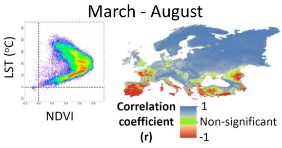
3.1. LST–NDVI Correlation Dynamics

In order to explore long-term pan-European correlations between LST and NDVI, their values were firstly mapped over the spatial domain of interest. Long-term (2000–2017) averages of higher daytime LST and NDVI for the entire seasonal study period (March–August) and the two sub-seasons (March–May and June–August) were created. Figure 2A,E,I generally indicate higher mean daytime LST values along the Mediterranean region in southern Europe that gradually decreased toward the higher latitudes. From June–August, the mean temperature range was 0.5 to 55 °C (with a mean of 26 °C), compared to a range of −12 to 37.5 °C (with a mean of 12.4 °C) from March–May. NDVI (Figure 2B,F,J) was characterized by overall higher values from June–August (range = −0.18 to 0.91, mean = 0.66) than from March–May (range = −0.19 to 0.81, mean = 0.42), with a substantial increase in northern and eastern Europe. Negative NDVI values indicate snow-covered pixels. Pairs of LST and NDVI maps were used to create density scatterplots (Figure 2C,G,K). In these plots, red and yellow colors represent higher pixel concentrations. For the entire period (Figure 2C), two distinct trends can be identified: one with a negative slope and a second with a positive slope. The strengths of these opposite correlations changed with the sub-period considered. A dominant positive correlation was observed during the spring months (Figure 2G). In contrast, during the summer months, most of the domain was characterized by a negative correlation (Figure 2K). The spatial distribution of r_lst–ndvi also varied between seasons (Figure 2D,H,L). For the entire period, most of the European region was characterized by a significant positive LST–NDVI relationship, with negatively-correlated areas only in the Mediterranean region and the Caucasus Mountains. From March–May, the positive relationship was even more pronounced across the continent. The warmer June–August sub-season reflected a different spatial pattern: the southern half of the study region showed mostly negative r_lst–ndvi values. However, mountainous areas (i.e., the Alps and the Carpathian Mountains) and the northern latitudes showed non-significant r_lst–ndvi correlation, with patches of positive values.

3.2. Biome-Specific LST–NDVI Relations

As noted above, seven biomes were involved in the current study: tundra; boreal forest/taiga; temperate forest; temperate conifer forest; temperate grassland, savanna, and shrubland; Mediterranean forest, woodland, and scrub; and desert and xeric shrubland (Figure 1). The biome-specific relations between LST and NDVI were highly diverse among the various biomes and throughout the entire study period (Figure 3). The northern biomes with the lowest temperature values (Tundra and Taiga) showed a constant positive relationship between LST and NDVI. The temperate biomes (broadleaf and mixed forests, conifer forests, and grasslands) were characterized by shifting trends between seasons (positive relationships from March–May that turned negative from June–August). The biomes with higher temperatures (Mediterranean forest and desert) typically had a negative LST–NDVI relationship throughout the entire studied timeframe.

Table 1. Percent of positive, negative, and non-significant pixels covering each of the biomes from March–August, March–May, and June–August. Bold values indicate values higher than 30%.

	rlst–ndvi
	Positive Correlation	Negative Correlation	Non-Significant Pixels
	(%)	(%)	(%)
March–August
Tundra	96	4	0
Boreal forest/taiga	100	0	0
Temperate broadleaf and mixed forest	89	5	6
Temperate conifer forest	92	4	4
Temperate grassland, savanna, and shrubland	75	9	16
Mediterranean forest, woodland, and scrub	23	66	11
Desert and xeric shrubland	16	71	13
March–May
Tundra	75	15	10
Boreal forest/taiga	99	0	1
Temperate broadleaf and mixed forest	97	1	2
Temperate conifer forest	96	1	3
Temperate grassland, savanna, and shrubland	96	1	3
Mediterranean forest, woodland, and scrub	44	32	24
Desert and xeric shrubland	52	10	38
June–August
Tundra	57	4	39
Boreal forest/taiga	60	1	39
Temperate broadleaf and mixed forest	5	64	31
Temperate conifer forest	13	42	45
Temperate grassland, savanna, and shrubland	0	97	3
Mediterranean forest, woodland, and scrub	0	94	6
Desert and xeric shrubland	1	88	11

shows r_lst–ndvi relations as percent of pixels that displayed each trend type (positive, negative, and non-significant). Overall, during the entire period (March–August), most of the biomes—65% of the study area—displayed a significant positive relationship. The Mediterranean and desert biomes, with a negative correlation, covered only 19% of the area (Figure 2D). During the spring season (March–May), 80% of the European domain—across all biomes—showed the dominance of significant positive relations. Exceptions were the Mediterranean forest and desert biomes, where the positive correlation covered about half of the area with relatively high coverage of non-significant pixels (Figure 2H). However, the summer season (June–August) featured a shift when 56% of the European area showed negative correlation values, 19% had positive values, and 25% of the pixels were non-significant (Figure 2L). Tundra and boreal forest/taiga were the only biomes that demonstrated a majority of significantly positive LST–NDVI relationships (57% and 60% of their total areas, respectively). The rest of the biomes were characterized by a large areal coverage of negative r_lst–ndvi values, except the temperate conifer forest biome which typically showed a larger portion of non-significant r_lst–ndvi values (45% of its area).

4. Discussion

This project explored the spatial and seasonal distributions of LST–NDVI relations as indicators of VGLFs, while distinguishing between water and energy limitation factors at the pan-European scale. Further, the project intended to link the LST–NDVI relations and the European biomes. To accomplish this goal, long-term (2000–2017) MODIS-derived LST and NDVI variables were obtained. Since the study covered a rather large continental scale, positive and negative correlations between LST and NDVI were observed in different regions of the domain and at different sub-seasonal periods. From a detailed analysis of these relationships, it can be inferred that when water is the limiting factor for vegetation growth during the summer season in the study area’s low latitudes, the LST–NDVI correlations are typically negative. However, when energy is the limiting factor for vegetation growth, as is the case at the northern latitudes or high elevations areas (especially at the beginning of the growing season), LST and NDVI correlations are positive. The correlation signs—either negative, positive, or non-significant—varied between different seasons and biomes. For the spring months, March–May, most of the areas of all biomes showed a positive correlation. During the summer months, June–August, most of the areas of the biomes changed to negative correlations, but the northern biomes of tundra and taiga mostly continued to display positive correlations. Large areas of non-significant correlations were also observed. These findings led to the following discussions.

4.1. Energy Balance Perspective

The spatial distribution of LST–NDVI relationships can also be examined from the perspective of the energy balance [38,39]. In rural areas, vegetation generally has a lower albedo than non-vegetated terrain in the same region, due to its spectral characteristics (vegetation cover) and its 3D structure. This 3D structure due to tree canopies leads to multiple scattering, increasing the shortwave radiation. Thus, longwave radiation is trapped, resulting in increased net longwave radiation [40]. Therefore, because of their lower albedo, the vegetated areas store more energy in the form of net radiation than the surrounding non-vegetated areas [38]. Part of this energy is stored in the surface, increasing its temperature (LST). This leads to a temperature gradient between the surface and lower atmosphere, and part of this energy is used to evaporate water, increasing turbulent latent heat flux. Evaporative cooling depends on the available energy [41], the landscape heterogeneity [42], as well as the type of vegetation and the soil moisture conditions. While evaporative cooling over grassland might exceed that over forest at times of ample soil moisture, the reverse is likely to occur under conditions of low soil moisture [43,44,45].

Generally, in southern latitudes (especially in arid/semi-arid areas) and the mid-latitudes during the summer period, solar radiation is high, leading to higher air temperature. During the daytime, high LST (and therefore high saturation water vapor pressure) is observed, whereas atmospheric water vapor pressure is usually low. Therefore, a vegetated surface in these cases is more likely to use a great part of the incoming energy to evaporate water. The higher the water availability (e.g., precipitation, irrigation), the higher the latent heat flux. Since the dominant type of vegetation is broadleaf, stomatal resistance is low, further contributing to high latent heat flux. Therefore, in these cases, the incoming energy in vegetated areas is mainly used to evaporate water, despite the lower albedo of vegetated areas. Conversely, the incoming energy in non-vegetated areas is stored in the respective surface, leading to the increase of temperature. For this reason, the LST in non-vegetated areas is usually higher than the LST of the surrounding vegetated areas. Pixels corresponding to vegetated areas (high NDVI) are expected to have a lower LST than the pixels that correspond to non-vegetated areas (low NDVI), which leads to a revised LST–NDVI correlation (Figure 2D,H,L).

Conversely, in northern latitudes, both the solar radiation and the air temperature are generally low. In general, where low LST (and therefore lower stomatal resistance) is observed, the relative humidity is consequently higher, and the air is close to saturation. Furthermore, in northern latitude areas, where boreal forest/taiga and tundra dominate, the respective stomatal resistance is expectedly high. Therefore, a relatively low latent heat flux is expected for vegetated areas in these regions. The net incoming energy in the form of radiation is stored in the vegetation canopies, increasing the respective LST. A small part of this energy is transported to the atmosphere as sensible heat flux due to the low-temperature gradient between the surface and air temperature in these latitudes. The mechanism is the same for the surrounding non-vegetated areas (no latent heat flux and low sensible heat flux). Thus, the incoming energy is stored in the surfaces, with higher storage in vegetated areas because the net incoming energy is higher due to the lower albedo. The higher heat storage in vegetated areas results in a higher LST than in non-vegetated ones. Consequently, pixels corresponding to vegetated areas (high NDVI) are expected to have a higher LST than the pixels corresponding to non-vegetated areas (low NDVI), which leads to a positive LST–NDVI correlation (Figure 2D,H,L). Finally, in the mid-latitudes and transition zones, as well as regions that are characterized by mixed-land-cover types, a combination of the above cases is expected, where both seasonality and water availability effects are most prominent.

4.2. European Biomes and Vegetation Growth-Limiting Factors

Two concerns were raised in this work regarding climate change and land-use changes: how will biome extents vary and how will the LST–NDVI relationships be affected. Parmesan [46] reviewed the ecological effects of climate change on phenology and species range shifts, and Watson et al. [47] estimated the vulnerability of ecoregions under climate change. In turn, Eigenbrod et al. [48] showed that the vulnerability of ecosystems to climate changes that induce biome shift depends on habitat intactness and on the scale on which intactness is estimated. In a study of European vegetation, Thuiller et al. [49] revealed that species distribution shifts triggered by climate change threaten plant biodiversity. In particular, species loss and turnover were found to be mainly determined by just two climatic variables: temperature and precipitation. In our approach, these are represented by LST and NDVI, respectively. For the coming decades, climate projections generally indicate an increase of temperature (thus, of LST) and a complex pattern of precipitation changes (thus, of NDVI). Therefore, plant species are expected to shift within and between biomes.

Since the relative strength of the different VGLFs might change, a major issue regards estimating future vegetation stress. Summer droughts in particular are expected to increase in the coming decades in Europe [50], possibly modifying the role of the different VGLFs and strengthening water limitation (and thus negative LST–NDVI relations). In turn, this is expected to lead to more severe summer fires and a drastic increase in the summer burned area [51]. Such estimates, based on empirical models, are rooted in the effects of the different VGLFs and can thus be affected by changes in the role of the different limiting factors, as expressed, for example, by the LST–NDVI correlations studied here. During the past years, for example, unexpected summer fires plagued northern European regions. A deeper understanding and modeling of the response of VGLFs and of the vegetation itself to the changing climate conditions is thus needed.

4.3. Relation to LST–NDVI Models

Previous studies, mostly limited in area and observation period, revealed a strong negative correlation between LST and NDVI. Based on this prevailing assumption, several vegetation/drought/stress indices were developed and widely applied. The hypothesis behind this assumption was the synergetic effect of water availability and energy effect on vegetation: less water and higher temperature promote vegetation stress and vice versa [26]. Hence, this naive model used only the ratio between LST and NDVI, acquired from the NOAA/AVHRR imagery, for mapping drought over Papua New Guinea and Mongolia [52,53]. A widely-used index based on the negative LST–NDVI relation is the Vegetation Health Index (VHI), developed by Kogan [54] as a proxy characterization of vegetation health or a combined estimation of moisture and thermal conditions. The index originally used long-term data from the NOAA-AVHRR spacecraft and has recently been used with the Visible Infrared Imaging Radiometer Suite (VIIRS) spectral bands [55] as well. VHI has been applied on a regional scale in many areas around the world [56,57,58], but has also been proposed as a global drought index [55,59,60,61]. Global coverage of the VHI is updated weekly on an official NOAA webpage (https://www.star.nesdis.noaa.gov/smcd/emb/vci/VH/vhbrowse.php).

Another spectral index that relies on an empirical parameterization of negative relations between LST and NDVI is the Temperature Vegetation Dryness Index (TVDI) [62,63]. This index is based on the location of a pixel in the LST–NDVI triangle or trapezoid-shaped scatterplot that associates higher LST with less evaporation, while higher NDVI values are identified with higher vegetation cover. This index has been applied to a vast number of sites all over the world, including Europe, as listed in Petropoulos et al. [64]. Wang and Dickinson [5] have reservations about using TVDI in northern latitudes and cold areas where temperatures, as a major control of latent heat flux, are mostly positively related to evaporation. Garcia et al. [65] examined the performance of the TVDI in a spatially heterogeneous region in southern Spain using MODIS imagery. They revealed that the index successfully assessed the water pressure deficit only under water-limited conditions and failed under energy-limited conditions.

Since droughts occur mostly in southern latitudes, these indices were developed with the implicit assumption that NDVI and LST are always and everywhere negatively correlated. Due to their simplicity, such as LST–NDVI-based models, they are widely accepted and commonly used. Furthermore, the availability of long-term remote sensing images at different spatial and temporal resolutions enabled the easy application of these models. In areas where water is ultimately the limiting factor for vegetation growth throughout the year, this assumption is apparently correct. However, these indices have been applied globally, even in regions and periods where the correlation is positive or non-significant.

5. Conclusions

In the current work, LST is a proxy for near-surface air temperature and NDVI is related to precipitation. The analysis of the correlations between these two biophysical variables provides information on how they vary in space and time and how they are related to each other. When energy is the limiting factor for vegetation growth, as in the case of northern latitudes and high elevations, significant positive correlations exist. Under water availability constraints, on the other hand, significant negative correlations are observed. During spring months, most of the domain is characterized by significant positive correlations that become significantly negative toward the summer, except for the northernmost regions. This behavior can be explained by taking into account the energy partitioning between latent and sensible heat flux, mainly regulated by surface albedo and temperature, as well as by air temperature.

The spatial distribution of the LST and NDVI correlation was found to be in line with previous studies that addressed large-scale climatic constraints but primarily relied on ground-based measurements and models. Long-term and global coverage of Earth-observed imagery from space provides a reliable dataset for biome mapping and ecological models. Predicted climate change will lead to an increase of temperature in the coming decades (i.e., increased LST), as well as a complex pattern of precipitation changes (i.e., changes of NDVI), thus shifts in plant species locations are expected causing redistribution of biomes.

The current project demonstrates that the drought/vegetation/stress indices, based on the prevalent hypothesis of a negative correlation between LST and NDVI, are also spatially and temporally dependent. Consequently, they are not valid in regions where energy is the limiting factor or during specific periods of the year. Furthermore, their results are doubtful when the correlations are statistically non-significant. Consequently, it is essential to re-examine this assumption and restrict applications of such an approach only to areas and periods in which negative correlations are observed.

References

1. Greenberg, J.A.; Santos, M.J.; Dobrowski, S.Z.; Vanderbilt, V.C.; Ustin, S.L. Quantifying environmental limiting factors on tree cover using geospatial data. PLoS ONE 2015, 10, e0114648. [Google Scholar] [CrossRef]
2. Bellard, C.; Bertelsmeier, C.; Leadley, P.; Thuiller, W.; Courchamp, F. Impacts of climate change on the future of biodiversity. Ecol. Lett. 2012, 15, 365–377. [Google Scholar] [CrossRef] [Green Version]
3. Churkina, G.; Running, S.W. Contrasting climatic controls on the estimated productivity of global terrestrial biomes. Ecosystems 1998, 1, 206–215. [Google Scholar] [CrossRef]
4. Nemani, R.R.; Keeling, C.D.; Hashimoto, H.; Jolly, W.M.; Piper, S.C.; Tucker, C.J.; Myneni, R.B.; Running, S.W. Climate-driven increases in global terrestrial net primary production from 1982 to 1999. Science 2003, 300, 1560–1563. [Google Scholar] [CrossRef]
5. Wang, K.C.; Dickinson, R.E. A review of global terrestrial evapotranspiration: Observation, modeling, climatology, and climatic variability. Rev. Geophys. 2012, 50, RG2005. [Google Scholar] [CrossRef]
6. Fensholt, R.; Langanke, T.; Rasmussen, K.; Reenberg, A.; Prince, S.D.; Tucker, C.; Scholes, R.J.; Le, Q.B.; Bondeau, A.; Eastman, R.; et al. Greenness in semi-arid areas across the globe 1981–2007—An earth observing satellite based analysis of trends and drivers. Remote Sens. Environ. 2012, 121, 144–158. [Google Scholar] [CrossRef]
7. Mutiibwa, D.; Strachan, S.; Albright, T. Land surface temperature and surface air temperature in complex terrain. IEEE J. Sel. Top. Appl. Earth Obs. Remote Sens. 2015, 8, 4762–4774. [Google Scholar] [CrossRef]
8. Phan, T.N.; Kappas, M.; Nguyen, K.T.; Tran, T.P.; Tran, Q.V.; Emam, A.R. Evaluation of MODIS land surface temperature products for daily air surface temperature estimation in northwest Vietnam. Int. J. Remote Sens. 2019, 40, 5544–5562. [Google Scholar] [CrossRef]
9. Zeng, L.L.; Wardlow, B.D.; Tadesse, T.; Shan, J.; Hayes, M.J.; Li, D.R.; Xiang, D.X. Estimation of daily air temperature based on MODIS land surface temperature products over the corn belt in the US. Remote Sens. 2015, 7, 951–970. [Google Scholar] [CrossRef]
10. Camberlin, P.; Martiny, N.; Philippon, N.; Richard, Y. Determinants of the interannual relationships between remote sensed photosynthetic activity and rainfall in tropical Africa. Remote Sens. Environ. 2007, 106, 199–216. [Google Scholar] [CrossRef] [Green Version]
11. Ding, M.J.; Zhang, Y.L.; Liu, L.S.; Zhang, W.; Wang, Z.F.; Bai, W.Q. The relationship between NDVI and precipitation on the Tibetan plateau. J. Geogr. Sci. 2007, 17, 259–268. [Google Scholar] [CrossRef]
12. Kang, L.J.; Di, L.P.; Deng, M.X.; Shao, Y.Z.; Yu, G.N.; Shrestha, R. Use of geographically weighted regression model for exploring spatial patterns and local factors behind NDVI-precipitation correlation. IEEE J. Sel. Top. Appl. Earth Obs. Remote Sens. 2014, 7, 4530–4538. [Google Scholar] [CrossRef]
13. Prihodko, L.; Goward, S.N. Estimation of air temperature from remotely sensed surface observations. Remote Sens. Environ. 1997, 60, 335–346. [Google Scholar] [CrossRef]
14. Sun, L.; Sun, R.; Li, X.W.; Liang, S.L.; Zhang, R.H. Monitoring surface soil moisture status based on remotely sensed surface temperature and vegetation index information. Agric. For. Meteorol. 2012, 166, 175–187. [Google Scholar] [CrossRef]
15. Wan, Z.; Wang, P.; Li, X. Using MODIS land surface temperature and normalized difference vegetation index products for monitoring drought in the southern great plains, USA. Int. J. Remote Sens. 2004, 25, 61–72. [Google Scholar] [CrossRef]
16. Anbazhagan, S.; Paramasivam, C.R. Statistical correlation between land surface temperature (LST) and vegetation index (NDVI) using multi-temporal landsat tm data. Int. J. Adv. Earth Sci. Eng. 2016, 5, 333–346. [Google Scholar]
17. Ferrelli, F.; Cisneros, M.A.H.; Delgado, A.L.; Piccolo, M.C. Spatial and temporal analysis of the LST-NDVI relationship for the study of land cover changes and their contribution to urban planning in Monte Hermoso, Argentina. Doc. D Anal. Geogr. 2018, 64, 25–47. [Google Scholar] [CrossRef] [Green Version]
18. Tan, K.C.; Lim, H.S.; MatJafri, M.Z.; Abdullah, K. A comparison of radiometric correction techniques in the evaluation of the relationship between LST and NDVI in landsat imagery. Environ. Monit. Assess. 2012, 184, 3813–3829. [Google Scholar] [CrossRef]
19. Vorovencii, I. A multi-temporal landsat data analysis of land use and land cover changes on the land surface temperature. Int. J. Environ. Pollut. 2015, 56, 109–128. [Google Scholar] [CrossRef]
20. Wang, H.; Li, X.B.; Long, H.L.; Xu, X.; Bao, Y. Monitoring the effects of land use and cover type changes on soil moisture using remote-sensing data: A case study in China’s Yongding River basin. Catena 2010, 82, 135–145. [Google Scholar] [CrossRef]
21. Nemani, R.R.; Running, S.W. Estimation of regional surface-resistance to evapotranspiration from NDVI and thermal-IR AVHRR data. J. Appl. Meteorol. 1989, 28, 276–284. [Google Scholar] [CrossRef]
22. Stisen, S.; Sandholt, I.; Norgaard, A.; Fensholt, R.; Eklundh, L. Estimation of diurnal air temperature using msg seviri data in West Africa. Remote Sens. Environ. 2007, 110, 262–274. [Google Scholar] [CrossRef]
23. Han, L.J.; Wang, P.X.; Yang, H.; Liu, S.M.; Wang, J.D. Study on NDVI-TS space by combining LAI and evapotranspiration. Sci. China Ser. D Earth Sci. 2006, 49, 747–754. [Google Scholar] [CrossRef]
24. Dall’Olmo, G.; Karnieli, A. Monitoring phenological cycles of desert ecosystems using NDVI and LST data derived from NOAA-AVHRR imagery. Int. J. Remote Sens. 2002, 23, 4055–4071. [Google Scholar] [CrossRef]
25. Holzman, M.E.; Rivas, R.; Piccolo, M.C. Estimating soil moisture and the relationship with crop yield using surface temperature and vegetation index. Int. J. Appl. Earth Obs. Geoinf. 2014, 28, 181–192. [Google Scholar] [CrossRef]
26. Carlson, T.N.; Petropoulos, G.P. A new method for estimating of evapotranspiration and surface soil moisture from optical and thermal infrared measurements: The simplified triangle. Int. J. Remote Sens. 2019, 40, 7716–7729. [Google Scholar] [CrossRef]
27. Schultz, P.A.; Halpert, M.S. Global analysis of the relationships among a vegetation index, precipitation and land-surface temperature. Int. J. Remote Sens. 1995, 16, 2755–2777. [Google Scholar] [CrossRef]
28. Lambin, E.F.; Ehrlich, D. The surface temperature-vegetation index space for land cover and land-cover change analysis. Int. J. Remote Sens. 1996, 17, 463–487. [Google Scholar] [CrossRef]
29. Nemani, R.; Running, S. Land cover characterization using multitemporal red, near-IR, and thermal-IR data from NOAA/AVHRR. Ecol. Appl. 1997, 7, 79–90. [Google Scholar]
30. Tateishi, R.; Ebata, M. Analysis of phenological change patterns using 1982–2000 advanced very high resolution radiometer (AVHRR) data. Int. J. Remote Sens. 2004, 25, 2287–2300. [Google Scholar] [CrossRef]
31. Julien, Y.; Sobrino, J.A.; Verhoef, W. Changes in land surface temperatures and NDVI values over europe between 1982 and 1999. Remote Sens. Environ. 2006, 103, 43–55. [Google Scholar] [CrossRef]
32. Karnieli, A.; Bayasgalan, M.; Bayarjargal, Y.; Agam, N.; Khudulmur, S.; Tucker, C.J. Comments on the use of the vegetation health index over Mongolia. Int. J. Remote Sens. 2006, 27, 2017–2024. [Google Scholar] [CrossRef]
33. Sun, D.L.; Kafatos, M. Note on the ndvi-lst relationship and the use of temperature-related drought indices over North America. Geophys. Res. Lett. 2007, 34. [Google Scholar] [CrossRef]
34. Karnieli, A.; Agam, N.; Pinker, R.T.; Anderson, M.; Imhoff, M.L.; Gutman, G.G.; Panov, N.; Goldberg, A. Use of NDVI and land surface temperature for drought assessment: Merits and limitations. J. Clim. 2010, 23, 618–633. [Google Scholar] [CrossRef]
35. Marzban, F.; Sodoudi, S.; Preusker, R. The influence of land-cover type on the relationship between NDVI-LST and LST-T-air. Int. J. Remote Sens. 2018, 39, 1377–1398. [Google Scholar] [CrossRef]
36. Olson, D.M.; Dinerstein, E.; Wikramanayake, E.D.; Burgess, N.D.; Powell, G.V.N.; Underwood, E.C.; D’Amico, J.A.; Itoua, I.; Strand, H.E.; Morrison, J.C.; et al. Terrestrial ecoregions of the world: A new map of life on earth. Bioscience 2001, 51, 933–938. [Google Scholar]
37. Stockli, R.; Vidale, P.L. European plant phenology and climate as seen in a 20-year AVHRR land-surface parameter dataset. Int. J. Remote Sens. 2004, 25, 3303–3330. [Google Scholar] [CrossRef]
38. Chrysoulakis, N.; Grimmond, S.; Feigenwinter, C.; Lindberg, F.; Gastellu-Etchegorry, J.P.; Marconcini, M.; Mitraka, Z.; Stagakis, S.; Crawford, B.; Olofson, F.; et al. Urban energy exchanges monitoring from space. Sci. Rep. 2018, 8, 11498. [Google Scholar] [CrossRef]
39. Wilson, K.; Goldstein, A.; Falge, E.; Aubinet, M.; Baldocchi, D.; Berbigier, P.; Bernhofer, C.; Ceulemans, R.; Dolman, H.; Field, C.; et al. Energy balance closure at fluxnet sites. Agric. For. Meteorol. 2002, 113, 223–243. [Google Scholar] [CrossRef]
40. Gastellu-Etchegorry, J.P.; Lauret, N.; Yin, T.G.; Landier, L.; Kallel, A.; Malenovsky, Z.; Al Bitar, A.; Aval, J.; Benhmida, S.; Qi, J.B.; et al. Dart: Recent advances in remote sensing data modeling with atmosphere, polarization, and chlorophyll fluorescence. IEEE J. Sel. Top. Appl. Earth Obs. Remote Sens. 2017, 10, 2640–2649. [Google Scholar] [CrossRef]
41. Moderow, U.; Aubinet, M.; Feigenwinter, C.; Kolle, O.; Lindroth, A.; Molder, M.; Montagnani, L.; Rebmann, C.; Bernhofer, C. Available energy and energy balance closure at four coniferous forest sites across Europe. Theor. Appl. Climatol. 2009, 98, 397–412. [Google Scholar] [CrossRef] [Green Version]
42. Stoy, P.C.; Mauder, M.; Foken, T.; Marcolla, B.; Boegh, E.; Ibrom, A.; Arain, M.A.; Arneth, A.; Aurela, M.; Bernhofer, C.; et al. A data-driven analysis of energy balance closure across fluxnet research sites: The role of landscape scale heterogeneity. Agric. For. Meteorol. 2013, 171, 137–152. [Google Scholar] [CrossRef]
43. Bonan, G.B. Forests and climate change: Forcings, feedbacks, and the climate benefits of forests. Science 2008, 320, 1444–1449. [Google Scholar] [CrossRef] [PubMed]
44. Baldocchi, D.D.; Xu, L.K.; Kiang, N. How plant functional-type, weather, seasonal drought, and soil physical properties alter water and energy fluxes of an oak-grass savanna and an annual grassland. Agric. For. Meteorol. 2004, 123, 13–39. [Google Scholar] [CrossRef]
45. Teuling, A.J.; Seneviratne, S.I.; Stockli, R.; Reichstein, M.; Moors, E.; Ciais, P.; Luyssaert, S.; van den Hurk, B.; Ammann, C.; Bernhofer, C.; et al. Contrasting response of European forest and grassland energy exchange to heatwaves. Nat. Geosci. 2010, 3, 722–727. [Google Scholar] [CrossRef]
46. Parmesan, C. Ecological and evolutionary responses to recent climate change. Ann. Rev. Ecol. Evol. Syst. 2006, 37, 637–669. [Google Scholar] [CrossRef]
47. Watson, J.E.M.; Iwamura, T.; Butt, N. Mapping vulnerability and conservation adaptation strategies under climate change. Nat. Clim. Chang. 2013, 3, 989–994. [Google Scholar] [CrossRef]
48. Eigenbrod, F.; Gonzalez, P.; Dash, J.; Steyl, I. Vulnerability of ecosystems to climate change moderated by habitat intactness. Glob. Chang. Biol. 2015, 21, 275–286. [Google Scholar] [CrossRef]
49. Thuiller, W.; Lavorel, S.; Araujo, M.B.; Sykes, M.T.; Prentice, I.C. Climate change threats to plant diversity in europe. Proc. Natl. Acad. Sci. USA 2005, 102, 8245–8250. [Google Scholar] [CrossRef]
50. Vautard, R.; Gobiet, A.; Sobolowski, S.; Kjellstrom, E.; Stegehuis, A.; Watkiss, P.; Mendlik, T.; Landgren, O.; Nikulin, G.; Teichmann, C.; et al. The European climate under a 2 degrees C global warming. Environ. Res. Lett. 2014, 9, 034006. [Google Scholar] [CrossRef]
51. Turco, M.; Rosa-Canovas, J.J.; Bedia, J.; Jerez, S.; Montavez, J.P.; Llasat, M.C.; Provenzale, A. Exacerbated fires in mediterranean europe due to anthropogenic warming projected with non-stationary climate-fire models. Nat. Commun. 2018, 1–9, 3821. [Google Scholar] [CrossRef] [PubMed]
52. Bayarjargal, Y.; Karnieli, A.; Bayasgalan, M.; Khudulmur, S.; Gandush, C.; Tucker, C.J. A comparative study of noaa-avhrr derived drought indices using change vector analysis. Remote Sens. Environ. 2006, 105, 9–22. [Google Scholar] [CrossRef]
53. McVicar, T.R.; Bierwirth, P.N. Rapidly assessing the 1997 drought in Papua New Guinea using composite AVHRR imagery. Int. J. Remote Sens. 2001, 22, 2109–2128. [Google Scholar] [CrossRef]
54. Kogan, F.N. Application of vegetation index and brightness temperature for drought detection. Adv. Space Res. 1995, 15, 91–100. [Google Scholar] [CrossRef]
55. Kogan, F.; Guo, W. Early detection and monitoring droughts from NOAA environmental satellites. In Use of Satellite and In-Situ Data to Improve Sustainability; Kogan, F., Powell, A.M., Fedorov, O., Eds.; Springer: Berlin/Heidelberg, Germany, 2011; p. 11. [Google Scholar]
56. Amalo, L.F.; Hidayat, R.; Sulma, S. Analysis of agricultural drought in East Java using vegetation health index. Agrivita 2018, 40, 63–73. [Google Scholar] [CrossRef]
57. Bento, V.A.; Trigo, I.F.; Gouveia, C.M.; DaCamara, C.C. Contribution of land surface temperature (TCI) to vegetation health index: A comparative study using clear sky and all-weather climate data records. Remote Sens. 2018, 10, 1324. [Google Scholar] [CrossRef]
58. Skakun, S.; Kussul, N.; Shelestov, A.; Kussul, O. The use of satellite data for agriculture drought risk quantification in ukraine. Geomat. Nat. Hazards Risk 2016, 7, 901–917. [Google Scholar] [CrossRef]
59. Kogan, F. Early drought detection, monitoring and assessment of crop losses from space: Global approach—art. No. 641209. In Disaster Forewarning Diagnostic Methods and Management; Kogan, F., Habib, S., Hegde, V.S., Matsuoka, M., Eds.; SPIE: Bellingham, WA, USA, 2006; Volume 6412, p. 41209. [Google Scholar]
60. Kogan, F.N. Global drought watch from space. Bull. Am. Meteorol. Soc. 1997, 78, 621–636. [Google Scholar] [CrossRef]
61. Kogan, F.N. World droughts in the new millennium from AVHRR-based vegetation health indices. EOS 2002, 83, 557–563. [Google Scholar] [CrossRef]
62. Carlson, T. An overview of the “triangle method” for estimating surface evapotranspiration and soil moisture from satellite imagery. Sensors 2007, 7, 1612–1629. [Google Scholar] [CrossRef]
63. Sandholt, I.; Rasmussen, K.; Andersen, J. A simple interpretation of the surface temperature/vegetation index space for assessment of surface moisture status. Remote Sens. Environ. 2002, 79, 213–224. [Google Scholar] [CrossRef]
64. Petropoulos, G.; Carlson, T.N.; Wooster, M.J.; Islam, S. A review of T-S/VI remote sensing based methods for the retrieval of land surface energy fluxes and soil surface moisture. Prog. Phys. Geogr. 2009, 33, 224–250. [Google Scholar] [CrossRef]
65. Garcia, M.; Fernandez, N.; Villagarcia, L.; Domingo, F.; Puigdefaabregas, J.; Sandholt, I. Accuracy of the temperature-vegetation dryness index using MODIS under water-limited vs. Energy-limited evapotranspiration conditions. Remote Sens. Environ. 2014, 149, 100–117. [Google Scholar] [CrossRef]
Figure 1. European biomes within the study area based on the World Wide Fund for Nature (WWF)–Terrestrial Ecoregions of the World website (https://www.worldwildlife.org/publications/terrestrial-ecoregions-of-the-world).
Remotesensing 11 02406 g001
Figure 2. (A,E,I) Average land surface temperature (LST) from March–August, March-May, and June–August, respectively; (B,F,J) Average normalized difference vegetation index (NDVI) for the respective periods; (C,G,K) LST–NDVI scatterplots for the respective periods; (D,H,L) Correlation coefficients for LST and NDVI for the respective periods.
Remotesensing 11 02406 g002
Figure 3. LST–NDVI scatterplots for each biome from March–August, March–May, and June–August.
Remotesensing 11 02406 g003