Article

Combining Evapotranspiration and Soil Apparent Electrical Conductivity Mapping to Identify Potential Precision Irrigation Benefits

by
Mallika A. Nocco
1,6,*,
Samuel C. Zipper
2,
Eric G. Booth
3,4,
Cadan R. Cummings
5,
Steven P. Loheide II
4 and
Christopher J. Kucharik
1,3
1
Nelson Institute Center for Sustainability and the Global Environment, University of Wisconsin-Madison, 1710 University Ave., Madison, WI 53726, USA
2
Kansas Geological Survey, University of Kansas, 1930 Constant Ave, Lawrence, KS 66047, USA
3
Department of Agronomy, University of Wisconsin-Madison, 1575 Linden Dr., Madison, WI 53706, USA
4
Department of Civil and Environmental Engineering, University of Wisconsin-Madison, 1415 Engineering Dr., Madison, WI 53706, USA
5
Department of Soil, Water, and Climate, University of Minnesota-Twin Cities, 1991 Upper Buford Circle, St. Paul, MN 55108, USA
6
Department of Land, Air, and Water Resources, University of California, Davis; One Shields Avenue, Davis, CA 95616, USA
*
Author to whom correspondence should be addressed.
Remote Sens. 2019, 11(21), 2460; https://doi.org/10.3390/rs11212460
Submission received: 6 September 2019 / Revised: 16 October 2019 / Accepted: 16 October 2019 / Published: 23 October 2019

Abstract

:
Precision irrigation optimizes the spatiotemporal application of water using evapotranspiration (ET) maps to assess water stress or soil apparent electrical conductivity (ECa) maps as a proxy for plant available water content. However, ET and ECa maps are rarely used together. We developed high-resolution ET and ECa maps for six irrigated fields in the Midwest United States between 2014–2016. Our research goals were to (1) validate ET maps developed using the High-Resolution Mapping of EvapoTranspiration (HRMET) model and aerial imagery via comparison with ground observations in potato, sweet corn, and pea agroecosystems; (2) characterize relationships between ET and ECa; and (3) identify potential precision irrigation benefits across rotations. We demonstrated the synergy of combined ET and ECa mapping for evaluating whether intrafield differences in ECa correspond to actual water use for different crop rotations. We found that ET and ECa have stronger relationships in sweet corn and potato rotations than field corn. Thus, sweet corn and potato crops may benefit more from precision irrigation than field corn, even when grown rotationally on the same field. We recommend that future research consider crop rotation, intrafield soil variability, and existing irrigation practices together when determining potential water use, savings, and yield gains from precision irrigation.

Graphical Abstract

1. Introduction

Precision irrigation is an agricultural practice where irrigators optimize the spatiotemporal application of water to maximize yield and minimize environmental impacts, and can reduce water use by up to 50% compared to traditional irrigation systems [1,2]. Precision irrigators often use proximal surveys of soil apparent electrical conductivity (ECa) for decision support when applying water at the subfield scale [3]. Soil ECa is influenced by particle size distribution, organic matter content, and structure, which are all also drivers of soil hydraulic properties [4,5]. Ideally, proximal surveys of ECa are conducted prior to tilling, planting, and fertilization on recently drained soils near field capacity [6,7,8]. Under these survey conditions, ECa has been demonstrated to predict soil hydraulic properties (e.g., field capacity, plant available water content) and expose water-limited yield gaps on a variety of soil types around the world [4,9,10,11,12,13,14,15]. Though ECa is an informative proxy for soil hydraulic properties, irrigators still face challenges when making in-season management decisions because maps of ECa are only static indicators of plant available water content. To manage water more effectively, irrigators also require information on crop water use dynamics throughout the growing season.
One source of data on crop water use dynamics is in-season maps of evapotranspiration (ET) derived from aerial or satellite imagery. High-resolution maps of ET are useful for identifying portions of a field that are water-stressed. Transpiration is a physiological indicator of crop growth, as it is links the carbon and water cycles [16]. Differences in transpiration drive water availability patterns within a cropping system, generating “hot spots” or areas that are consistently under-or over-irrigated [17]. High-resolution maps of ET can expose irrigation hot spots integrating more biophysical information than crop water stress indicators based on canopy temperature alone [18]. Crops that are consistently under or over irrigated may exhibit low transpiration, which is a physiological indicator of either water or oxygen limitation [19]. However, in order to understand whether crops are consistently under or over irrigated, ET maps need to be compared with maps of plant available water content.
The comparison of high-resolution maps of ET, a dynamic indicator of crop water use, and ECa, a static indicator of plant available water content, may expose potential benefits and drawbacks to implementing precision irrigation for different crop rotations. Persistent patterns in the magnitude and variability of ET within a cropping system can indicate differences in soil texture and plant available water content [18,20]. However, the spatial relationships between ET and plant available water content may change with different crop rotations because of canopy structure, root distribution, physiology, and breeding. As such, we hypothesize that there may be differences in the amount of ‘precision’ required to optimize water use in irrigated, rotational cropping systems. We test this hypothesis by quantifying the relationships between high resolution estimates of ET and ECa across different crop rotations and fields in a humid agricultural region with coarse soils. A strong relationship between ET and ECa indicates that intrafield differences in crop water use are related to plant available water content, which would be the most pronounced in fields with heterogenous soils. This scenario is a favorable opportunity for precision irrigation intervention—increasing irrigation inputs over the coarsest portions of the field should result in higher transpiration rates. Alternatively, limited relationships between ET and ECa indicate that soil properties are not driving crop physiology and greater spatial control of irrigation will not impact transpiration. Soil properties will not drive crop physiology through their effects on water availability in (1) fields that have extremely spatially homogenous soils; and/or (2) fields that are being influenced by external management factors such as uneven fertilizer distribution. The greater the variability in intrafield soil texture and hydraulic properties on a uniformly irrigated field, the stronger the relationships should be between ET and ECa.
We explore ET and ECa relationships across different traditionally irrigated crop rotations to assess potential benefits from precision irrigation interventions on coarse soils. Our research goals were to (1) develop ET maps for irrigated rotational crops using and validating the High-Resolution Mapping of EvapoTranspiration (HRMET) model, aerial imagery, and ground observations; (2) characterize relationships between water use and availability across crop rotations within the same fields and across different crop types (e.g., potato, sweet corn, field corn, peas) using ET and ECa maps; (3) identify potential precision irrigation benefits on both a field and crop basis.

2. Materials and Methods

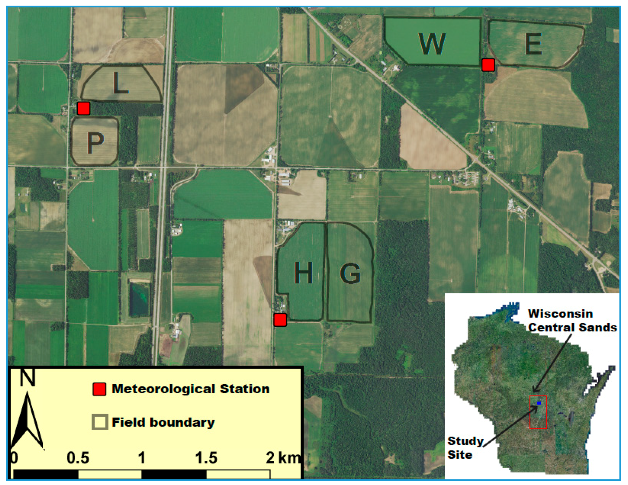
2.1. Site Description

The northern Great Lakes states of Wisconsin, Michigan, and Minnesota are known for having a humid climate, relatively abundant groundwater supply, and rapidly expanding irrigated agriculture [21]. Coarse-grained glacial aquifers throughout these states support coldwater trout streams, lakes, and wetlands [22]. The Wisconsin Central Sands (WCS, Figure 1) is a relatively small (6400 km2) ecological region in the U.S. northern Great Lakes states where the coarse soils and groundwater irrigation have facilitated intense agricultural productivity that helps make Wisconsin the fourth leading producer of fresh market and processing vegetables in the United States [23]. Groundwater is strongly connected to the 1000 km of headwater streams, 80 lakes, and abundant wetlands in the WCS, where freshwater conservation, surface water health, and agricultural sustainability are stakeholder priorities [24]. Recent modeling in the WCS has demonstrated that reducing both the frequency and magnitude of groundwater pumping for irrigation could diminish adverse impacts on adjacent surface waters [25,26]. Precision irrigation could reduce the frequency and magnitude of groundwater pumping, while maintaining or increasing agricultural productivity in the WCS and similar areas.
We used aerial remote sensing to map ET, proximal sensing to map ECa, and collected complementary ground observations from six commercial fields (denoted H, G, P, L, E, W) in the WCS that had an average planted area of 23 ha for the 2014–2016 growing seasons (Figure 1). We collected aerial imagery and ground observations in partnership with Isherwood Farms, a 600-ha, sixth-generation family farm growing irrigated potatoes, sweet corn, field corn, and peas (Figure 1). Isherwood Farms does not currently use precision irrigation methods (e.g., variable-rate irrigation) and uniformly applies irrigation over each field from a center pivot based on weather monitoring, soil conditions, and crop observations. In these agroecosystems, irrigation typically commences at the end of June and supplements rainfall as 6–15 mm events applied every 2–3 days. All six fields are relatively flat and well drained, with sand, loamy sand, and sandy loam soil textures. Agronomic information for each crop, field, and growing season is presented in Table 1.

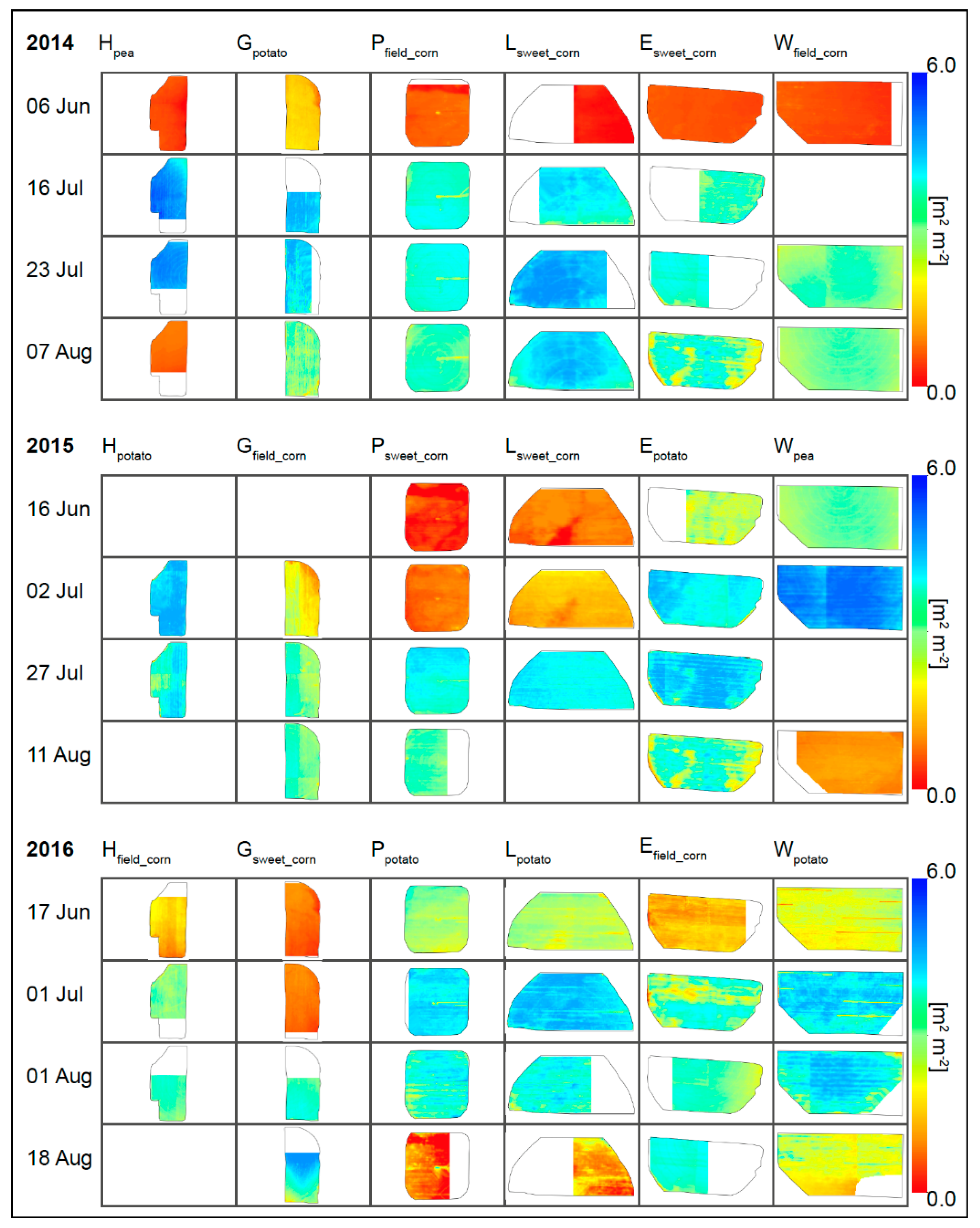
2.2. Remotely Sensed Maps of ET

High-resolution maps of ET can be created using satellite or aircraft imagery from multiple wavelength bands to estimate canopy surface temperature and reflectance-based vegetation indices [17,18,27]. Canopy surface temperature, aerodynamic temperature, and vegetation indices form the basis for several energy balance models that either explicitly represent vegetation and soil as two sources within a pixel [28,29,30] or combine vegetation and soil together as a single source within a pixel [31,32]. The majority of these remotely sensed ET models require the designation of ‘hot/dry’ vs. ‘cold/wet’ pixels to indicate the minimum and maximum limits of ET within an image and facilitate contextual scaling of ET values between these limits [28,31,33,34]. Though this type of contextual scaling approach requires less input data and processing [27] and reduces uncertainty arising from meteorological inputs [33], it has unique drawbacks for precision agricultural applications where fields are relatively homogenous and endmember pixels are challenging to identify [18]. Moreover, in irrigated cropping systems, agricultural fields are maintained to minimize water stress; which makes it especially challenging to identify ‘hot/dry’ pixels in the relatively small image domain (<1 km2) needed to capture high-resolution data. To meet the unique challenges of mapping ET for irrigated agroecosystems, we used the High-Resolution Mapping of EvapoTranspiration (HRMET) model [18] to estimate ET using airborne imagery and local meteorological forcing. HRMET is a one-dimensional (vertical), process-based energy balance model that uses canopy characteristics, land surface temperature, and meteorological data to estimate latent heat flux as the residual of the energy balance, which can then be converted to ET [18]. HRMET uses a two-source algorithm to estimate available energy for vegetation and soil and a single-source iterative calculation of sensible heat flux at a pixel, which eliminates the need for contextual scaling using ‘hot/dry’ or ‘cold/wet’ pixels and makes HRMET well suited for precision agricultural applications. For more information about the theory and structure of HRMET, please refer to Zipper and Loheide (2014) [18]. HRMET is an open-source model and the code for R and MATLAB are available at https://github.com/samzipper/HRMET.
Here, we apply HRMET in a gridded manner over our domain using remotely sensed maps of canopy surface temperature (Section 2.3), LAI and h (Section 2.5), and local meteorological data (Section 2.6) as inputs. We ran simulations at a spatial resolution of 2 m in order to match the resolution of the canopy surface temperature data. The inputs derived from micrometeorological stations required for HRMET include air temperature (°C), wind speed (m s−1), air vapor pressure (kPa), and atmospheric pressure (kPa). Finally, HRMET requires emissivity and albedo values for both vegetation and soil to calculate the energy balance. We used emissivity values of 0.94 and 0.95 for vegetation and soil; assuming a standard deviation of 0.01 because there is a small range in emissivity for these surfaces [16]. We used albedo values of 0.20 and 0.11 for vegetation and irrigated sandy soils maintained near field capacity; assuming a standard deviation of 0.05 [16]. Though HRMET does not require calibration and has already been validated for field corn in Wisconsin via comparison to the Shuttleworth–Wallace approach [18], we provide additional validation from this study in potato, sweet corn, and pea-pearl millet cropping systems.
We assessed the influence of error from all model inputs on ET estimates using a Monte Carlo approach [35]. The mean and standard deviation of all spatial, meteorological, and empirical inputs were used to create an ensemble of input data based on the standard normal distribution. We then solved HRMET 300 times at each pixel with a randomly selected group of inputs for each permutation of HRMET. We conducted a power analysis with field ‘P’ (the smallest field with the shortest model run time) to determine that 300 permutations were required to ensure stability. The 300 ET estimates were used to calculate the final mean and standard deviation of ET for each pixel. Combined, this permutation-based analysis led to 980,534,100 HRMET calculations for our 68 images with 3,268,447 pixels and 300 calculations pixel−1. Each HRMET input and its data source are described in Table 2.

2.3. Airborne Missions and Data Processing
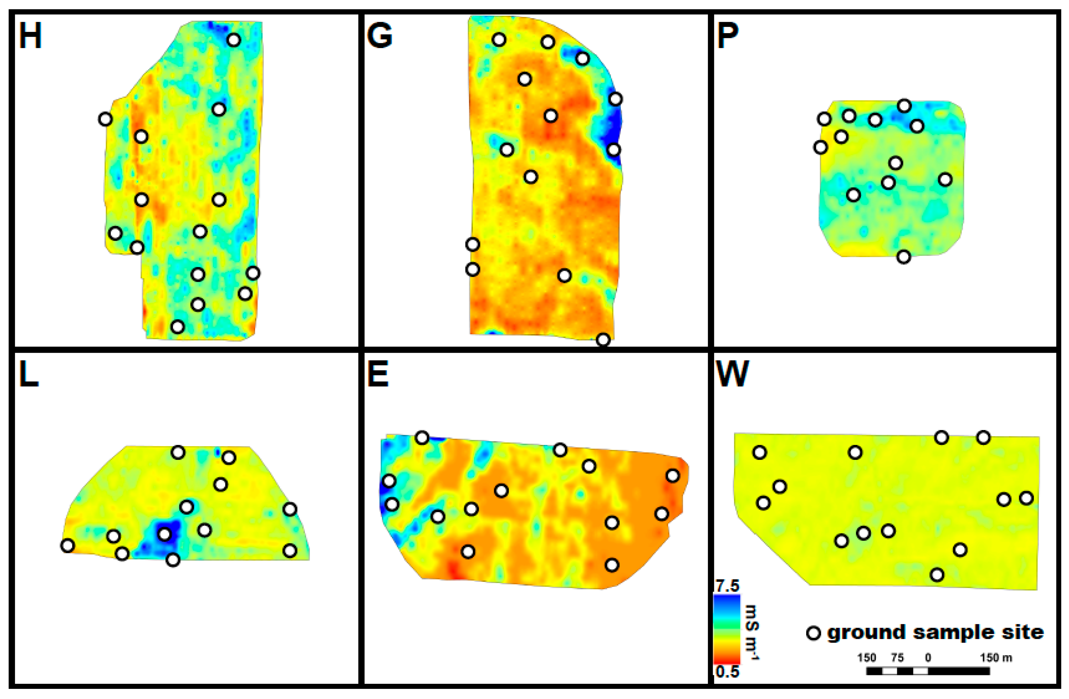
Twelve airborne missions were conducted during the growing seasons of 2014–2016 (4 per June–August) to capture data during different crop rotations and phenological stages (Table 3). We acquired thermal and multispectral imagery over six fields from equipment mounted on the underside of a single engine three-passenger Cessna aircraft. Though all attempts were made to have airborne missions coincide with cloud-free days, some images were cut off or discarded because of cloud interference. The thermal imagery was captured using a FLIR A320 thermal infrared imaging camera at a pixel size of 1–2 m based on flight elevation (FLIR Systems, Wilsonville, OR, USA). We performed atmospheric corrections using ThermaCAM Researcher Pro 2.7 software (FLIR systems, Wilsonville, OR, USA 2003), georeferenced the data to National Agricultural Imaging Program (NAIP) imagery, and mosaicked images using ArcMap 10 (ESRI, Redlands, CA, USA, 2010). We estimated the mean and standard deviation of surface temperature data using a 25-pixel moving window approach [18].
We collected multispectral images using a six-sensor Tetracam Multi Camera Array (MCA) system (Tetracam Inc., Los Angeles, CA, USA) at a pixel size of 0.6–0.8 m with multiband sensors centered at 450, 570, 620, 650, 670, and 860 nm. Multispectral images were coregistered using Pixelwrench (Tetracam Inc., Los Angeles, CA, USA 2001) and georeferenced to NAIP imagery. We converted digital numbers captured by the MCA system to surface reflectance values using the control points method described by Kang et al., (2016) [36]. In brief, we chose 3–5 stable control points (e.g., healthy green grass, concrete parking area) present in each image and collected ten spectral reflectance measurements at 1 nm resolution from each point using an ASD handheld spectroradiometer at the end of the 2016 field season (Analytical Spectral Devices, Inc., Boulder, CO, USA). We averaged spectral reflectance measurements at 10 nm intervals matching each MCA band in order to build linear relationships between digital numbers and surface reflectance values at each control point, which we used to convert digital numbers to surface reflectance values. All digital number-surface reflectance fits had R2 values >0.71. We spatially aggregated images to 5 m resolution to represent the canopy scale of indices with both plants and soil in each pixel [27]. We computed the Enhanced Vegetation Index (EVI) [37,38] from aggregated images using surface reflectance data. Overpass time, image collection height, and meteorological conditions for each mission are detailed in Table 2.

2.4. ECa Surveys

We partnered with a precision agricultural consulting firm to conduct proximal surveys of ECa prior to cultivation when soil moisture was at or near field capacity on 13 April 2015 for fields P, L, E, and W and 21 April 2016 for fields H and G (Precision Waterworks LLC, Plainfield, WI, USA). Measurements were collected using the Veris Soil EC 3100 (Veris Technologies, Salina, KS, USA), which is an instrument that estimates bulk shallow (ECa_sh, integrated over 0–0.3 m soil depth) and deep (ECa_dp, integrated over 0–0.9 m) ECa via electromagnetic induction [39]. We collected ECa point data from 18-m wide transects and made a measurement every 2–3 m along each transect. All ECa survey data were temperature corrected to 25 °C using the model of Sheets and Hendrickx (1995) corrected by Corwin and Lesch (2005) [40,41]. We interpolated ECa survey data (n = 215–230 ha−1) to a 2-m grid for all six fields (n = 2100–2200 ha−1) using ordinary kriging and spherical variogram models [42,43] in ArcMap 10 (ESRI, Redlands, CA, USA, 2010; Figure 2). A companion study established that these ECa_sh and ECa_dp maps predict particle size, soil organic matter, and field capacity from the six fields on Isherwood Farms in this study [9]. Thus, we use the same ECa maps as proxies for plant available water content. High ECa values within a field signify relatively higher plant available water, higher field capacity, greater silt and clay content, and higher soil organic matter, while low ECa values within a field signify relatively lower plant available water and greater sand content. Direct ECa comparisons are relative to each field in this study and a particular ECa value on one field does not necessarily indicate the same plant available water content at the same ECa value on another field.

2.5. Crop Phenology

We collected weekly measurements of leaf area index (LAI, m2 m−2) during the growing seasons of 2015–2016 using a LI-COR LAI-2200 plant canopy analyzer (LI-COR Inc., Lincoln, NE, USA). LAI measurements were collected under diffuse light conditions (e.g., sunrise or sunset) or clear skies. Scattering effects were removed for clear sky measurements using a bidirectional model [44] embedded in post-processing software (FV2200 2.0, LI-COR Inc., Lincoln, NE, USA). Weekly LAI measurements were collected within a 5-m radius of locations demarcated in Figure 2. Weekly measurements of canopy height (h) were collected within 3–4 days of each airborne mission at locations demarcated in Figure 2. We used smoothing splines in the MATLAB Curve Fitting Toolbox (MATLAB, 2015b) to interpolate LAI and h values to the date of each airborne mission.
Vegetation indices such as EVI have often been used to predict LAI and h for energy balance modeling using empirical relationships developed from ground-based measurements of phenology [45,46]. The relationships between EVI, LAI, and h in cropping systems are best represented by different simple functional forms including linear, power, and exponential fits with two or three coefficients [36]. We compiled all 2015–2016 spatially explicit LAI, h, and EVI values to generate models to predict LAI and h from EVI for field corn, sweet corn, potato, peas, and pearl millet (mid-season cover crop following peas). The data were fit using a nonlinear least squares regression approach with six possible functional forms (linear, power, and exponential with two or three coefficients). We chose the best functional form for each crop model of LAI or h based on minimizing RMSE values. We used a permutation-based approach [18] to estimate uncertainty in crop models of LAI and h for each remotely sensed image. We executed 50 permutations of LAI or h models for each crop data set, each time eliminating 5 random data points, fitting the remaining data, and using the eliminated points to determine the model fit; thereby generating 50 fitted LAI and h models for each crop. We then used the 50 different sets of model coefficients to fit LAI and h at each EVI pixel, generating mean and standard deviations of LAI and h for each image. Functional forms, coefficients, and goodness of fit statistics for each chosen LAI or h model are tabulated in Appendix A. LAI maps are presented for each mission in Figure 3.

2.6. Micrometeorology

Three micrometeorological weather stations were installed (Figure 1, ‘M’) adjacent to fields in 2013 according to the World Meteorological Organization guide for agrometeorological observations from fixed stations [47]. Instruments measuring precipitation (S-RGA-M0002; Onset Computer Corp., Bourne, MA, USA), temperature and relative humidity (S-THB-M002; Onset Computer Corp., Bourne, MA, USA), wind speed (S-WSB-M003; Onset Computer Corp., Bourne, MA, USA), and solar radiation (silicon pyranometer, S-LIB-M003; Onset Computer Corp., Bourne, MA, USA) were mounted on 2-m tripods over grass surfaces (M-TPB-KIT; Onset Computer Corp., Bourne, MA, USA). Measurements were collected every 10 min and recorded using a HOBO (Onset Computer Corp., Bourne, MA, USA) micro station data logger. We estimated cumulative reference ET (RET) as an index of evaporative demand for each growing season using micrometeorological data and American Society of Civil Engineers (ASCE) standardized equations for a uniform grass crop [48,49]. Isherwood Farms provided irrigation records, which were validated using soil moisture measurements and three additional rain gauges [50]. Two meteorological stations malfunctioned during the 2015 field season, so all 2015 values are derived from the station between fields ‘L’ and ‘P’. Cumulative precipitation, irrigation, and reference evapotranspiration for the 2014–2016 growing seasons are presented in Figure 4.
For airborne missions where the field or sweet corn canopy height exceeded 2 m, we used meteorological data from a 7.6 m high National Weather Service (NWS) cooperative observer station 4 km from the field site to run HRMET over the fields with crops >2 m. Wind speed measurements must be taken above canopy height when using HRMET, as sensible heat flux is calculated based on the gradient between surface canopy temperature and the air temperature above the canopy. The heights of wind speed measurements are standardized and adjusted using logarithmic profiles in the calculation of the friction velocity and aerodynamic resistance. We estimated uncertainty in meteorological inputs using data collected from all stations 30 min before and after the mean image collection time (6–7 data points/station) for each airborne mission. Because air temperature and solar radiation are time-dependent inputs, we estimated uncertainty using the standard deviation of the residuals from a linear regression of the one-hour time series.

2.7. Shuttleworth–Wallace Validation

We validated HRMET estimates of instantaneous ET (mm hr−1) for potato, sweet corn, and pea-pearl millet cropping systems via comparison to the Shuttleworth–Wallace model, which uses a dual-source approach that is ideal for both sparse and full canopy conditions and allowed us to generate hourly, point-based ET estimates appropriate for validating HRMET [51]. In addition to the phenological and meteorological inputs also required for HRMET, the Shuttleworth–Wallace model requires surface soil moisture and stomatal conductance inputs to estimate surface resistance. We collected surface soil moisture and stomatal conductance measurements during or immediately after airborne missions in 2015–2016. Within an hour of each airborne mission, we collected 7–10 measurements of stomatal conductance (SC-1 Leaf Porometer, Decagon Devices, Inc., Pullman, WA, USA) and 20 measurements of surface soil moisture (Thetaprobe ML2x, Delta-T Devices, Cambridge, UK) at 2–5 locations in potato, sweet corn, or pea-pearl millet agroecosystems. Stomatal conductance and surface soil moisture measurement locations were always chosen to coincide with LAI and h data collection locations demarcated in Figure 2. These measurements provided us with 2–5 validation points for each of the 8 airborne missions in 2015–2016. The number of validation points depended on the speed with which we could calibrate the porometer and move among calibration sites within an hour of the flight. Any Shuttleworth–Wallace points that did not have a complementary HRMET estimate (due to clouds) were eliminated from the validation, leaving 26 total validation points. The surface soil moisture measurements were used to calculate surface soil resistance using the method of Camillo and Gurney (1986) [52] and assuming a uniform saturated soil water content of 0.41 m3 m−3 for loamy sand [53]. We used a sunlight extinction model [16] to estimate total sunlit LAI and a big leaf approach to upscale stomatal conductance measurements to total bulk canopy resistance [51].

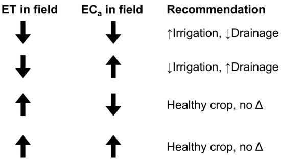
2.8. Relative Indices and Ordinal Correlation Analyses
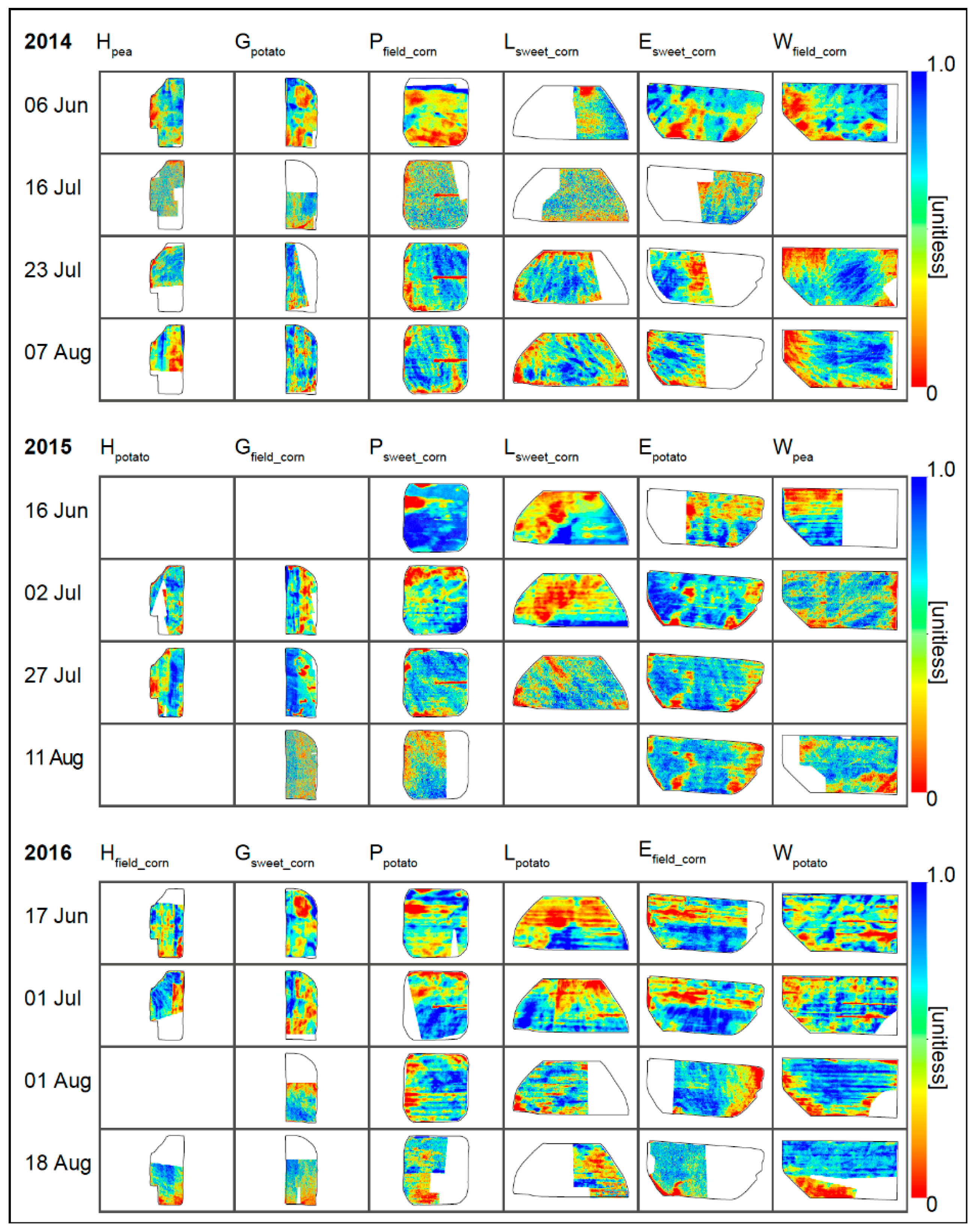
We used the relative ET index (ETR) [18] to examine intrafield variability in ET over different crop rotations. To calculate ETR, we linearly normalized mean ET rates to the 5th and 95th percentile for each mosaicked set of images for a single field on a given measurement date. Thus, an ETR value of 1 indicates the maximum ET rates within a field, while an ETR value of 0 indicates minimum ET rates within a field. To examine relationships between ETR and plant available water content across fields and rotations, we also linearly normalized shallow and deep ECa values for each field to the 5th and 95th percentile.
Though ET is a temporally variable process subject to external forcing (e.g., seasonality, weather), we are interested in understanding how its intrafield spatial variability and sensitivity to differences in soil properties responds to changes across different crop rotations. Thus, we used the normalized ETR index to examine the strength and direction of relationships with normalized ECa_sh and ECa_dp values within each field using ordinal correlation analyses on a per-pixel basis (n = 30,830–63,031 pixels per field). We built correlation coefficient matrices using Kendall’s tau coefficients. The Kendall’s tau coefficient is a nonparametric measure of correlation for ordinal, continuous data assuming a monotonic relationship [54]. Tau values range from −1 to 1, where −1 is a perfect negative relationship, 0 indicates no relationship, and 1 is a perfect positive relationship. Statistical significance was assessed at an alpha level of 0.001 for all correlations in this study. We assumed that the relationship between ET and ECa is monotonic in coarse soils, where ET limitation due to anoxic conditions is rare. Kendall’s tau correlation matrices have 4–5 variables per field including ECa_sh, ECa_dp, and average ETR for each crop grown between 2014–2016. We also examined the strength and direction of relationships between ECa_sh, ECa_dp, and ETR for potato, sweet corn, and field corn across all six fields using Kendall’s tau correlation coefficient matrices. There were not enough pea-pearl millet rotations to include in the analyses across all fields.
We also used ordinal correlation analyses to identify the relationships between ECa and ET across different crops and fields. Strong, significant correlations between ETR and ECa indicate greater potential precision irrigation benefits because relatively coarser portions of the field have lower ET rates due to water limitations not observed on relatively finer portions of the field. Precision irrigation would reduce the correlation between ETR and ECa by increasing water applied to coarser portions of the field. Thus, weak or nonexistent relationships between ETR and ECa indicate that either specific crop rotations or fields would not benefit from increased spatial control of irrigation applications.

3. Results

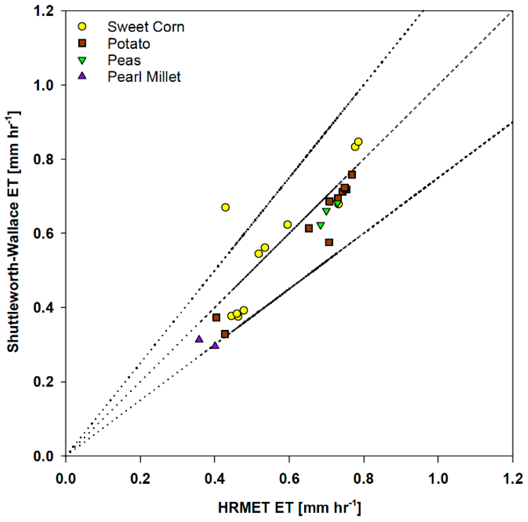
3.1. Validation of HRMET in Irrigated Potatoes, Sweet Corn, Peas, and Pearl Millet

Using aerial imagery, onsite meteorological data, and ground observations to drive HRMET was an effective approach for developing high-resolution maps of ET. HRMET performed comparably to the Shuttleworth–Wallace ET model (Figure 5). The slope of the linear relationship between the Shuttleworth–Wallace and HRMET models was 1.032, the RMSE was 0.074 mm hr−1, and the R2 value was 0.814 across all points (n = 26). Comparing across only potato validation points (n = 10), the slope of the linear relationship between the Shuttleworth–Wallace and HRMET models was 1.087, the RMSE was 0.038 mm hr−1, and the R2 value was 0.943. Comparing across only sweet corn validation points (n = 11), the slope of the linear relationship between the Shuttleworth–Wallace and HRMET models was 1.079, the RMSE was 0.102 mm hr−1, and the R2 value was 0.700. There are not enough validation points to separately compare pea (n = 3) and pearl millet (n = 2) crop validations.
HRMET performed well in both sparse and full canopy conditions. The validation included sparse canopy conditions during the June flights for sweet corn, potato, and peas as well as the August 2015 flight for pearl millet. Full canopy conditions were validated via the July flights for sweet corn, potato, and peas. Sparse canopy conditions during senescence were also validated for potato during the August 2015 and 2016 flights. In this study, HRMET estimates of ET were 0.1 mm hr−1 closer to Shuttleworth–Wallace estimates than they were in a rainfed field corn study in southern Wisconsin during a droughty year [18]. We suggest that the improved agreement between HRMET and Shuttleworth–Wallace in the WCS is attributed to the removal of water limitations as the Shuttleworth–Wallace model is intended to estimate ET from well-watered canopies [51,55].

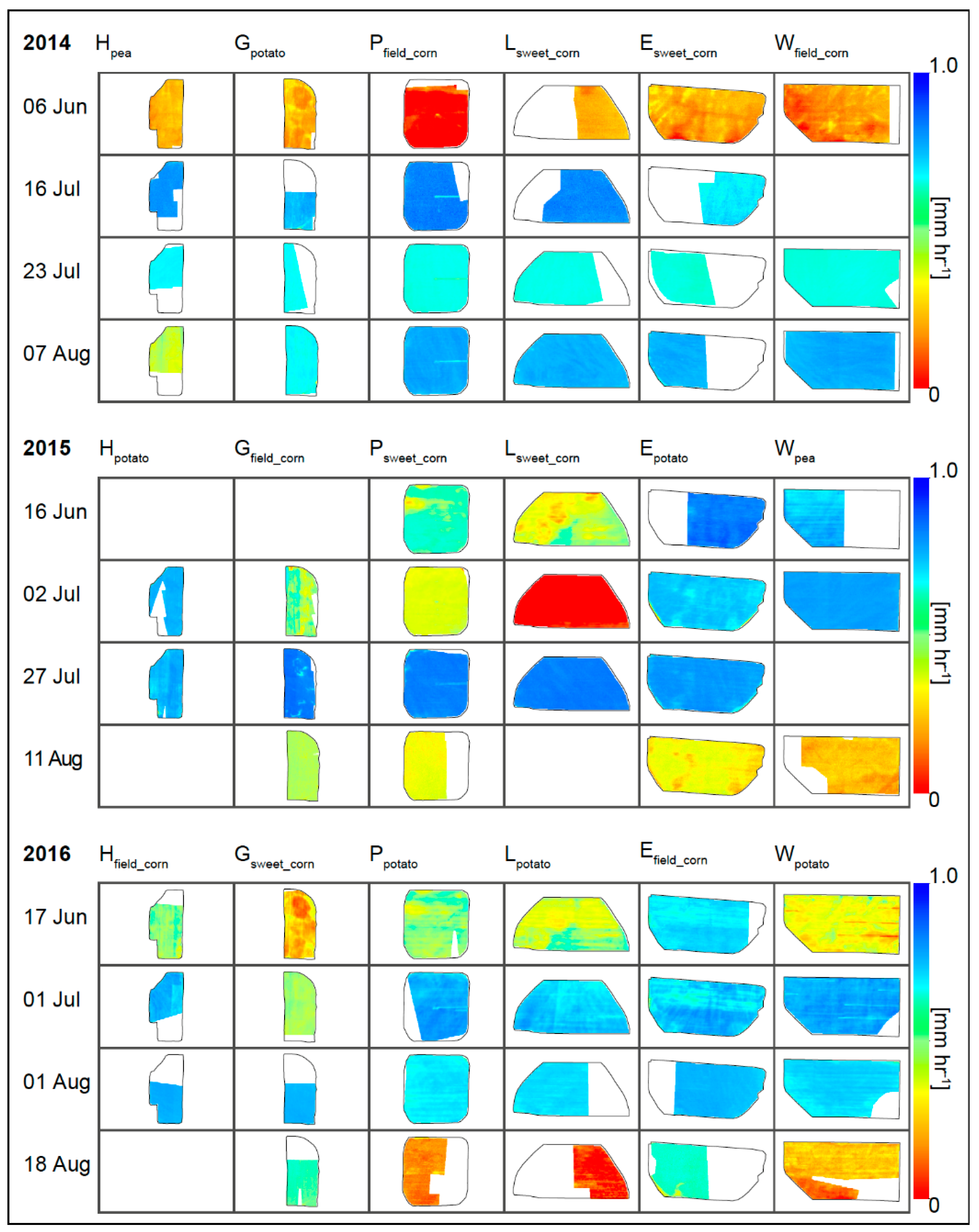
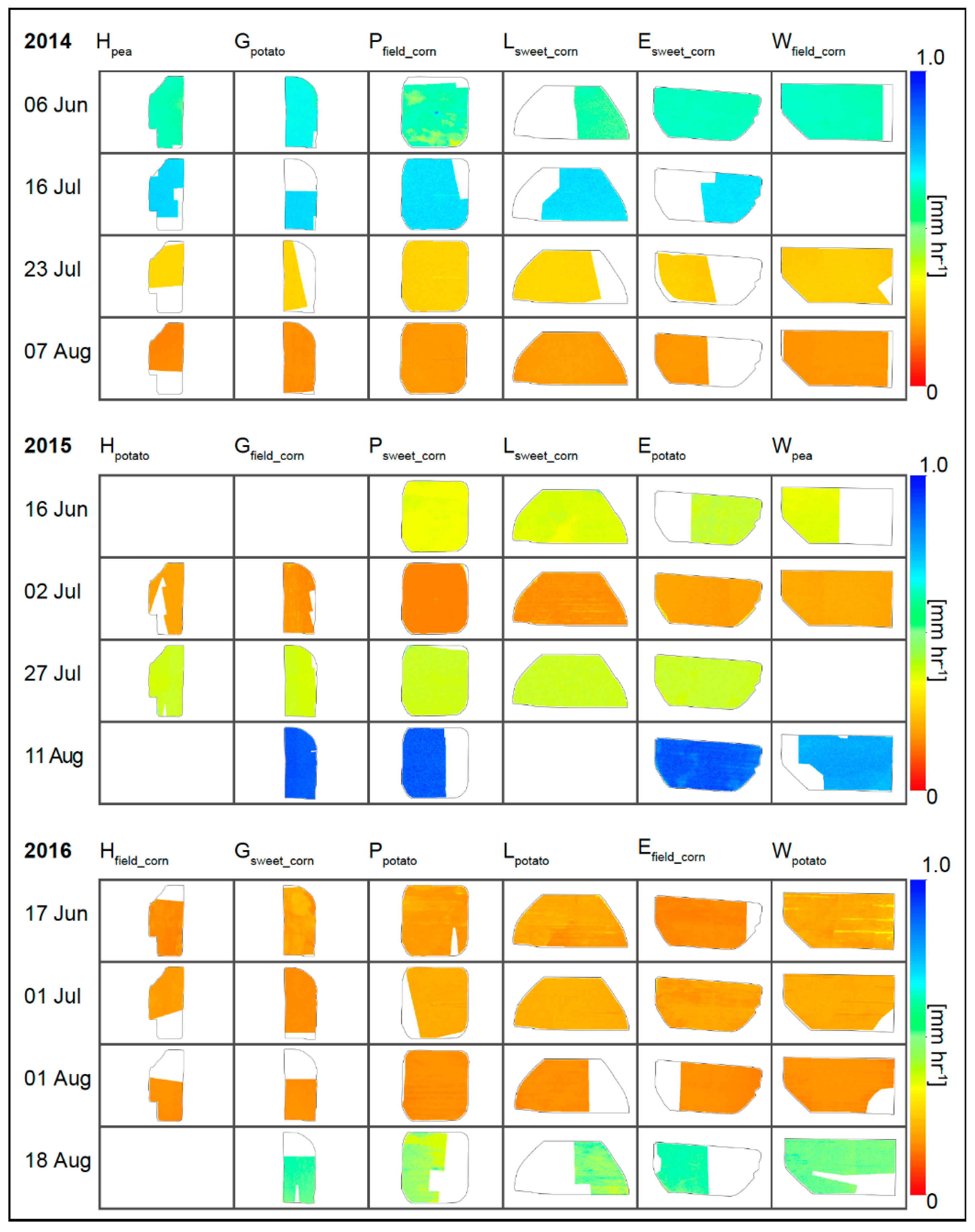
3.2. Uncertainty in Remotely-Sensed ET Estimates

We observed little to no spatial variability in the standard deviation of ET per pixel, indicating that the uncertainty of ET estimates is derived from the variability of meteorological data (Figure 6 and Figure 7). The uncertainty in per pixel ET estimates of 8 out of 12 missions was low and CVs averaged across all pixels and fields were 6–15%. The four airborne missions occurring on 11 August 2015, 6 June 2014, 18 August 2016, and 16 July 2014 had higher uncertainty in per pixel ET estimates with coefficients of variation (CVs) of 48, 46, 30, and 24% averaged across all pixels for all fields. These four dates also had the highest standard deviations in solar radiation (117–227 W m−2) observed across all 12 airborne missions (Table 2). Observationally, these were four missions where cloud conditions were rapidly changing and it was challenging to capture thermal and multiband imagery around intermittent cloud cover.

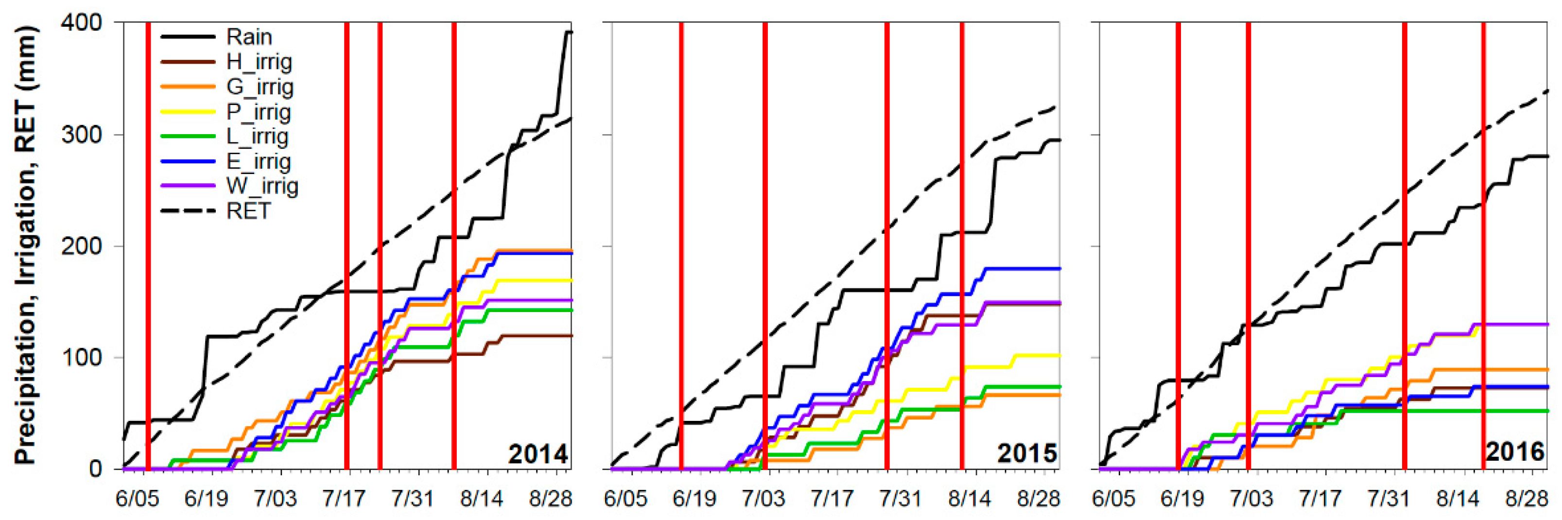
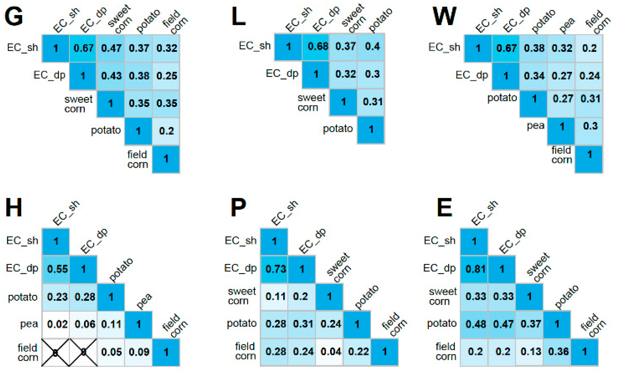
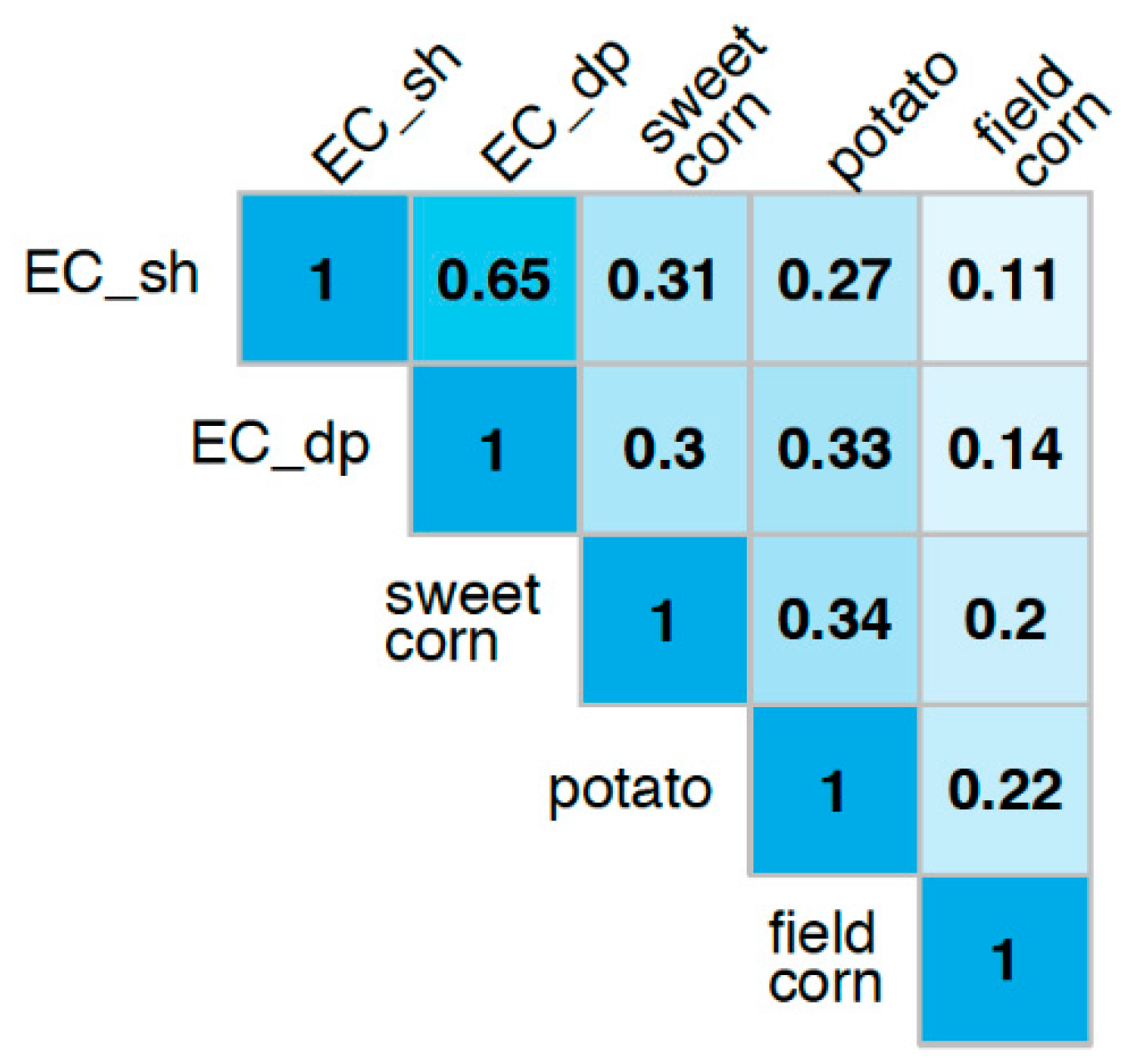
3.3. Relationships between Water Use and Availability

Relative ET (ETR) maps facilitate the comparison of intrafield variability in ET across airborne missions (Figure 8). Qualitatively, several of the ETR maps exhibit similar patterns to ECa maps (Figure 2), especially for airborne missions with limited canopy cover where soil evaporation dominates ET. There were significant correlations (p < 0.001) between ETR and ECa on each field with Kendall’s tau values ranging from 0.05–0.47 across all rotations (Figure 9) and across all six fields with a tau values of 0.27–0.33, 0.3–0.31, and 0.11–0.14 for potato, sweet corn, and field corn, respectively (Figure 10). We found that ETR had relatively similar correlation coefficients with both ECa_sh and ECa_dp across each rotation. Correlations between ETR and ECa were the strongest on fields E and G and the weakest on field H. These significant relationships between ETR and ECa indicate that subfield differences in plant available water content drive crop water use at the subfield scale. This means that precision irrigation interventions (e.g., variable rate irrigation using management zones) should provoke more efficient crop water use. Some potential precision water management recommendations based on strongly correlated measurements of ETR and ECa are highlighted in Table 4.
Interfield differences in ET were less than or equal to intrafield differences in ET with some key exceptions caused by phenology or water limitations (Table 5). Observable differences in LAI (Figure 3) aligned with interfield differences in ET during the 7 August 2014, 16 June 2015, 2 July 2015, 11 Aug 2015, 1 July 2016, and 18 August 2016 missions. Sweet corn was planted the latest in all three years and, consequently, had low LAI and ET in June and early July images. Senescing potato crops and pearl millet cover crops with only partial canopy cover limited ET in August images. In the absence of observable differences in phenology, water limitations likely caused interfield differences in ET on 6 June 2014 and 2 July 2015. During the 6 June 2014 mission, fields P and W had very similar LAI values for field corn (Figure 3), though field P was planted three days earlier than field W. Field P had a mean ET of 0.18 mm hr−1, while field W had a mean ET of 0.31 mm hr−1 (Table 5). Water limitation on field P may have resulted from an absence of rain in the four days preceding the 6 June 2014 mission, which took place prior to irrigation initiation. Likewise, during the 2 July 2015 mission, fields L and P had very similar LAI values for sweet corn (Figure 3), but field L had a mean ET of 0.12 mm hr−1, while field P had a mean ET value of 0.47 mm hr−1 (Table 5). Water limitation on field L may have resulted from an absence of rain and irrigation in the four days preceding the 2 July 2015 mission, as field L was irrigated on 2 July 2015 after the mission, while field P received 21 mm of irrigation over the four days prior to the flight.

4. Discussion

4.1. Potential Precision Irrigation Benefits Depend on Crop Rotation

Our findings suggest that precision irrigation benefits will be crop-specific, even on the same agricultural field. For example, variable rate irrigation guided by ECa mapping may lead to greater water conservation and productivity outcomes in potato and sweet corn rotations than field corn. In this study, potato and sweet corn rotations had stronger relationships between ETR and ECa than field corn on all six fields. Field corn may not be as responsive to precision irrigation as other crops because it has a deeper rooting profile than sweet corn and potatoes [56] and has also been genetically engineered over the past 50 years to have increased drought tolerance and improved water-use efficiency [57]. This idea of crop-specific precision irrigation applies where shallow-rooted, high water-demand crops are rotated with deep-rooted, water-efficient crops that may not be worth the time, cost, and effort required for precision irrigation interventions.

4.2. Potential Precision Irrigation Benefits Depend on Intrafield Soil Variability

Precision irrigation benefits will also depend on whether differences in plant available water content are significant enough to impact crop water use within a field. For example, ETR and ECa had strong relationships in pea-pearl millet rotations on field W, but were almost unrelated on field H, which has low variability in soil hydraulic properties [9]. A strong relationship between ETR and ECa indicates that the intrafield variability in plant available water content is significant enough to impact crop water use when irrigation is distributed uniformly over a field. Because the relationships between ETR and ECa were the strongest on fields E and G, we suggest that these fields have the most significant intrafield plant water content variability and would benefit the most from precision irrigation if the crop type was constant. These fields also have the strongest variability in soil texture, field capacity, and organic matter content [9]. Conversely, because field H had the weakest relationships between ETR and ECa, we argue that it offers a limited return on investment in precision irrigation interventions, regardless of the specific crop rotation. The coarse-textured, relatively homogenous soils in this study show minimal spatial variability in plant available water content which impacts impact crop water use within a field. We speculate that observing the relationships between ETR and ECa could be an even more powerful approach for informing irrigation management on fields with greater soil heterogeneity and more fine-grained soils than those in the Wisconsin Central Sands.

4.3. Potential Precision Irrigation Benefits Depend on Existing Irrigation Practices

Precision irrigation benefits will depend on existing conventional irrigation practices that amplify or diminish the spatial variability of crop water limitation. Irrigation practices already in place may diminish the observed variability in ET on a given field, which could potentially conceal or misinform the identification of precision irrigation benefits. For example, field L had a stronger relationship between ECa and ETR for potatoes and sweet corn than field P. Both fields L and P have strong relationships between ECa and soil hydraulic properties [9], are separated by only ~100 m, and were planted with sweet corn in 2015 and potatoes in 2016. However, field P received 28 and 78 mm yr−1 more irrigation than field L in 2015 and 2016, respectively. We suggest that the increased irrigation on field P may have irrigated the relatively finer-textured portions of the field at higher rates than necessary and washed out intrafield differences in ET. Alternatively, decreased irrigation on field L may have under-irrigated the relatively coarser-textured portions of the field and amplified intrafield differences in ET. Both fields may be candidates for precision irrigation based on their soil heterogeneity, however specific interventions would differ based on current irrigation practices.

4.4. Future Applications of HRMET

A long-term goal of regional water managers is to have high-resolution estimates of ET available for irrigators to use in real-time irrigation management. Analyses are underway to implement an integrated data fusion approach and create high-resolution (30-m) daily maps of ET in the WCS by fusing Landsat, MODIS, and GOES satellite imagery data [58,59]. However, acquiring frequent cloud-free satellite imagery of cropping systems is a significant and ongoing challenge in the midwestern United States [60]. Thus, satellite-derived ET estimates are gap-filled during cloudy periods using the “self-preservation” ratio of actual to reference ET (i.e., crop coefficients) [17,61]. High-resolution estimates of ET using HRMET could be especially useful for validating satellite-based daily ET estimates. Because it is possible to capture thermal images by avoiding clouds with the aid of a deft pilot, we were able to estimate ET on cloudy days that would present gaps in satellite data. Using the HRMET model in conjunction with thermal and multiband imagery collected via remotely piloted aircrafts could further provide even more flexibility around cloud cover in regions like the Midwest United States. Additionally, the Monte Carlo approach we used facilitates an improved understanding of which meteorological drivers contribute to the uncertainty of ET estimates on a given day. Recent studies are attempting to separate high-resolution satellite fusion estimates of daily ET from different crops in close proximity to one another [58]. These research efforts could be even more informative to water managers by incorporating meteorological uncertainty into ET estimates from different crops in close proximity. HRMET provides a valuable tool to understand whether the uncertainty of ET estimates is greater than the differences in ET between different crops in close proximity. For example, in this study, the uncertainty of instantaneous ET estimates within a crop type was always greater than the differences in ET between crop types. Thus, though it is possible to separate the ET estimates by crop type, the magnitude of the differences between crops may not always be significant. Understanding these uncertainties by crop type and land cover will help planners and policymakers manage stakeholder expectations from precision irrigation and other conservation interventions that rely on satellite data for decision support.

5. Conclusions

Precision irrigation is gaining traction as a water conservation strategy that could maximize crop production and water-use efficiency while minimizing environmental impacts. Maps of ECa, especially when paired with soil sampling or soil moisture monitoring, can help irrigators identify intrafield heterogeneity in plant available water content. Pairing ECa with maps of crop ET and the ETR index can further support irrigators in assessing the potential return on investment in precision irrigation technology for different fields and crops. We found that shallow-rooted crops like potatoes and sweet corn are more likely to benefit from precision interventions than deep-rooted crops bred for drought resistance (e.g., field corn). We also validated the HRMET model in potatoes, sweet corn, peas, and pearl millet, and demonstrated its usefulness for assessing crop water use and uncertainty in sandy, irrigated agroecosystems at the spatiotemporal scale necessary for validating future satellite-based efforts.
Combining high-resolution ECa and ET mapping could critically inform precision irrigation in rotational agroecosystems. Maps of crop ET and the ETR index can help irrigators assess the sensitivity of different crops to drought, develop irrigation management zones, and maximize the return on investment in precision irrigation technology. In this study, we demonstrated that relationships between dynamic crop water use (ETR) and plant available water content (ECa) are driven by (1) crop type, where shallow-rooted crops exhibit greater intrafield variability in water use; (2) intrafield soil physical variability, which needs to be significant enough to impact ET; and (3) existing irrigation management, which can amplify or diminish water limitations. Further studies are needed to assess long-term water savings, water use efficiency, and the yield potential of precision irrigation interventions in rotational agroecosystems.

Author Contributions

Conceptualization, M.A.N., S.C.Z, C.J.K., and S.P.L.I.; Methodology, M.A.N., S.C.Z., E.G.B., and C.R.C.; Software, S.C.Z., M.A.N., C.R.C., and E.G.B.; Validation, M.A.N. and S.C.Z.; Formal analysis, M.A.N.; Investigation, M.A.N. and C.J.K.; Resources, C.J.K., E.G.B., and S.P.L.I.; Writing—original draft preparation, M.A.N.; Writing—review and editing, M.A.N., S.C.Z., E.G.B., C.R.C., C.J.K., and S.P.L.I.; Visualization, M.A.N., E.G.B., and C.R.C.; Supervision, C.J.K. and S.P.L.I.; Project administration, M.A.N. and C.J.K.; Funding acquisition, M.A.N., C.J.K., and S.P.L.I.

Funding

The research described in this study has been funded in part by the United States Environmental Protection Agency (EPA) under the Science to Achieve Results (STAR) Graduate Fellowship Program. EPA has not officially endorsed this publication and the views expressed herein may not reflect the views of the EPA. Additionally, this work is a product of research funded by the Wisconsin Department of Natural Resources (WDNR), University of Wisconsin Consortium for Extension and Research in Agriculture and Natural Resources, the United States Department of Agriculture Sustainable Agriculture Research and Education program, and the Smith Family and Wisconsin Potato Industry Board Distinguished Graduate Fellowships, and the David H. Smith Conservation Research Fellowship.

Acknowledgments

We also acknowledge Isherwood Farms, Eric Kruger, Matthew Ruark, Noah Feinstein, George Kraft, John Panuska, Paige Frautschy, Christopher Ester, Amy Sandel Ester, and Logan Ebert for assistance with research development, manuscript review, experimental logistics, statistics, field work, and airborne campaigns. We would also like to acknowledge John Jorgensen, Jeffrey Oimoen, and Gary Vetterli at the WDNR Aeronautics Section for flight logistics and services.

Conflicts of Interest

The authors declare no conflict of interest.

Appendix A

Table A1. LAI-EVI and height-EVI fits.
Crop TypePhenological VariablenPrediction ModelCoefficients (Confidence Intervals)RMSER2
abc
Field cornLAI (m2 m−2)122 a x b 3.986
(3.581, 4.391)
1.308
(0.935, 1.681)
-1.1270.464
h (m)96 a x b + c 2.486
(1.951, 3.022)
1.471
(0.555, 2.387)
0.115
(−0.526, 0.755)
0.4980.632
Sweet cornLAI (m2 m−2)124 a x b 4.848
(4.496, 5.199)
1.323
(1.115, 1.531)
-0.7830.788
h (m)123 a x + b 2.369
(2.130, 2.609)
−0.1758
(−0.321, −0.031)
-0.3910.762
PotatoLAI (m2 m−2)209 a x b 4.675
(4.379, 4.971)
0.6257
(0.504, 0.748)
-1.1400.431
h (m)213 a b x 0.252
(0.2294 0.275)
0.7435
(0.620, 0.867)
-0.0900.412
PeasLAI (m2 m−2)29 a x + b 5.386
(5.036, 5.737)
−0.1658
(−0.412, 0.080)
-0.3270.974
h (m)29 a x + b 0.593
(0.561, 0.625)
1.266
(1.048, 1.483)
-0.0530.952
Pearl MilletLAI (m2 m−2)13 a x b 1.739
(0.526, 2.952)
0.393
(−0.148, 0.934)
-0.4010.393
h (m)12 a x b + c 3.633
(−11.680, 18.940)
4.743
(−0.969, 10.460)
0.111 (0.077, 0.145)0.0280.516

References

  1. Sadler, E.J.; Evans, R.G.; Stone, K.C.; Camp, C.R. Opportunities for conservation with precision irrigation. J. Soil Water Conserv. 2005, 60, 371–378. [Google Scholar]
  2. Delgado, J.A.; Bausch, W.C. Potential use of precision conservation techniques to reduce nitrate leaching in irrigated crops. J. Soil Water Conserv. 2005, 60, 379–387. [Google Scholar]
  3. Liakos, V.; Vellidis, G.; Tucker, M.; Lowrance, C.; Liang, X. A decision support tool for managing precision irrigation with center pivots. In Precision Agriculture’15; Wageningen Academic Publishers: Wageningen, The Netherlands, 2015; pp. 713–720. ISBN 9086862675. [Google Scholar]
  4. Rezaei, M.; Saey, T.; Seuntjens, P.; Joris, I.; Boënne, W.; Van Meirvenne, M.; Cornelis, W. Predicting saturated hydraulic conductivity in a sandy grassland using proximally sensed apparent electrical conductivity. J. Appl. Geophys. 2016, 126, 35–41. [Google Scholar] [CrossRef]
  5. Fortes, R.; Millán, S.; Prieto, M.H.; Campillo, C. A methodology based on apparent electrical conductivity and guided soil samples to improve irrigation zoning. Precis. Agric. 2015, 16, 441–454. [Google Scholar] [CrossRef]
  6. Neely, H.L.; Morgan, C.L.S.; Stanislav, S.; Rouze, G.; Shi, Y.; Thomasson, J.A.; Valasek, J.; Olsenholler, J. Strategies for soil-based precision agriculture in cotton. In Autonomous Air and Ground Sensing Systems for Agricultural Optimization and Phenotyping; International Society for Optics and Photonics: Bellingham, WA, USA, 2016; Volume 9866, p. 98660K. [Google Scholar]
  7. Pedrera-Parrilla, A.; Van De Vijver, E.; Van Meirvenne, M.; Espejo-Pérez, A.J.; Giráldez, J.V.; Vanderlinden, K. Apparent electrical conductivity measurements in an olive orchard under wet and dry soil conditions: Significance for clay and soil water content mapping. Precis. Agric. 2016, 17, 531–545. [Google Scholar] [CrossRef]
  8. Islam, A.; Ahuja, L.R.; Garcia, L.A.; Ma, L.; Saseendran, A.S. Modeling the effect of elevated co (2) and climate change on reference evapotranspiration in the semi-arid central great plains. Trans. ASABE 2012, 55, 2135–2146. [Google Scholar] [CrossRef]
  9. Nocco, M.A.; Ruark, M.D.; Kucharik, C.J. Apparent electrical conductivity predicts physical properties of coarse soils. Geoderma 2019, 335, 1–11. [Google Scholar] [CrossRef]
  10. Haghverdi, A.; Leib, B.G.; Washington-Allen, R.A.; Ayers, P.D.; Buschermohle, M.J. Perspectives on delineating management zones for variable rate irrigation. Comput. Electron. Agric. 2015, 117, 154–167. [Google Scholar] [CrossRef]
  11. Sudduth, K.A.; Kitchen, N.R.; Wiebold, W.J.; Batchelor, W.D.; Bollero, G.A.; Bullock, D.G.; Clay, D.E.; Palm, H.L.; Pierce, F.J.; Schuler, R.T. Relating apparent electrical conductivity to soil properties across the north-central USA. Comput. Electron. Agric. 2005, 46, 263–283. [Google Scholar] [CrossRef]
  12. Hedley, C.B.; Yule, I.J. Soil water status mapping and two variable-rate irrigation scenarios. Precis. Agric. 2009, 10, 342–355. [Google Scholar] [CrossRef]
  13. Hedley, C.B.; Yule, I.J. A method for spatial prediction of daily soil water status for precise irrigation scheduling. Agric. Water Manag. 2009, 96, 1737–1745. [Google Scholar] [CrossRef]
  14. Gooley, L.; Huang, J.; Page, D.; Triantafilis, J. Digital soil mapping of available water content using proximal and remotely sensed data. Soil Use Manag. 2014, 30, 139–151. [Google Scholar] [CrossRef]
  15. Ortuani, B.; Chiaradia, E.A.; Priori, S.; L’Abate, G.; Canone, D.; Comunian, A.; Giudici, M.; Mele, M.; Facchi, A. Mapping Soil Water Capacity Through EMI Survey to Delineate Site-Specific Management Units Within an Irrigated Field. Soil Sci. 2016, 181, 252–263. [Google Scholar] [CrossRef]
  16. Campbell, G.S.; Norman, J.M. An Introduction to Environmental Biophysics; Springer: Berlin/Heidelberg, Germany, 1998; ISBN 0387949372. [Google Scholar]
  17. Semmens, K.A.; Anderson, M.C.; Kustas, W.P.; Gao, F.; Alfieri, J.G.; McKee, L.; Prueger, J.H.; Hain, C.R.; Cammalleri, C.; Yang, Y. Monitoring daily evapotranspiration over two California vineyards using Landsat 8 in a multi-sensor data fusion approach. Remote Sens. Environ. 2016, 185, 155–170. [Google Scholar] [CrossRef] [Green Version]
  18. Zipper, S.C.; Loheide, S.P., II. Using evapotranspiration to assess drought sensitivity on a subfield scale with HRMET, a high resolution surface energy balance model. Agric. For. Meteorol. 2014, 197, 91–102. [Google Scholar] [CrossRef]
  19. Feddes, R.A.; Hoff, H.; Bruen, M.; Dawson, T.; de Rosnay, P.; Dirmeyer, P.; Jackson, R.B.; Kabat, P.; Kleidon, A.; Lilly, A. Modeling root water uptake in hydrological and climate models. Bull. Am. Meteorol. Soc. 2001, 82, 2797–2809. [Google Scholar] [CrossRef]
  20. Zipper, S.C.; Soylu, M.E.; Booth, E.G.; Loheide, S.P., II. Untangling the effects of shallow groundwater and soil texture as drivers of subfield-scale yield variability. Water Resour. Res. 2015, 51, 6338–6358. [Google Scholar] [CrossRef] [Green Version]
  21. Watson, K.A.; Mayer, A.S.; Reeves, H.W. Groundwater availability as constrained by hydrogeology and environmental flows. Groundwater 2014, 52, 225–238. [Google Scholar] [CrossRef]
  22. Kraft, G.J.; Clancy, K.; Mechenich, D.J.; Haucke, J. Irrigation effects in the northern lake states: Wisconsin central sands revisited. Groundwater 2012, 50, 308–318. [Google Scholar] [CrossRef]
  23. Wisconsin Department of Natural Resources. The Ecological Landscapes of Wisconsin: An Assessment of Ecological Resources and Guide to Planning Sustainable Management; PUB-SS_1131L2015; Wisconsin Department of Natural Resources: Madison, WI, USA, 2015.
  24. Kraft, G.J.; Mechenich, D.J. Groundwater Pumping Effects on Groundwater Levels, Lake Levels, and Streamflows in the Wisconsin Central Sands; Center for Watershed Science and Education, College of Natural Resources, University of Wisconsin-Stevens Point/Extension: Stevens Point, WI, USA, 2010. [Google Scholar]
  25. Bradbury, K.; Fienen, M.; Kniffin, M.; Krause, J.; Westenbroek, S.M.; Leaf, A.T.; Barlow, P.M. Groundwater Flow Model for the Little Plover River basin in Wisconsin’s Central Sands; Wisconsin Geological and Natural History Survey: Madison, WI, USA, 2017. [Google Scholar]
  26. Fienen, M.N.; Bradbury, K.R.; Kniffin, M.; Barlow, P.M. Depletion Mapping and Constrained Optimization to Support Managing Groundwater Extraction. Groundwater 2018, 56, 18–31. [Google Scholar] [CrossRef]
  27. Kustas, W.P.; Anderson, M.C.; Alfieri, J.G.; Prueger, J.H.; Geli, H.M.E.; Neale, C.M.U. Mapping evapotranspiration with high-resolution aircraft imagery over vineyards using one-and two-source modeling schemes. Hydrol. Earth Syst. Sci. 2016, 20, 1523. [Google Scholar]
  28. Norman, J.M.; Kustas, W.P.; Humes, K.S. Source approach for estimating soil and vegetation energy fluxes in observations of directional radiometric surface temperature. Agric. For. Meteorol. 1995, 77, 263–293. [Google Scholar] [CrossRef]
  29. Kustas, W.P.; Norman, J.M. A two-source energy balance approach using directional radiometric temperature observations for sparse canopy covered surfaces. Agron. J. 2000, 92, 847–854. [Google Scholar] [CrossRef]
  30. Yang, Y.; Shang, S. A hybrid dual-source scheme and trapezoid framework–based evapotranspiration model (HTEM) using satellite images: Algorithm and model test. J. Geophys. Res. Atmos. 2013, 118, 2284–2300. [Google Scholar] [CrossRef]
  31. Bastiaanssen, W.G.M.; Menenti, M.; Feddes, R.A.; Holtslag, A.A.M. A remote sensing surface energy balance algorithm for land (SEBAL). 1. Formulation. J. Hydrol. 1998, 212, 198–212. [Google Scholar] [CrossRef]
  32. Feng, J.; Wang, Z. A satellite-based energy balance algorithm with reference dry and wet limits. Int. J. Remote Sens. 2013, 34, 2925–2946. [Google Scholar] [CrossRef]
  33. Allen, R.G.; Tasumi, M.; Trezza, R. Satellite-based energy balance for mapping evapotranspiration with internalized calibration (METRIC)—Model. J. Irrig. Drain. Eng. 2007, 133, 380–394. [Google Scholar] [CrossRef]
  34. Timmermans, W.J.; Kustas, W.P.; Andreu, A. Utility of an automated thermal-based approach for monitoring evapotranspiration. Acta Geophys. 2015, 63, 1571–1608. [Google Scholar] [CrossRef]
  35. Serbin, S.P.; Singh, A.; McNeil, B.E.; Kingdon, C.C.; Townsend, P.A. Spectroscopic determination of leaf morphological and biochemical traits for northern temperate and boreal tree species. Ecol. Appl. 2014, 24, 1651–1669. [Google Scholar] [CrossRef] [Green Version]
  36. Kang, Y.; Özdoğan, M.; Zipper, S.C.; Román, M.O.; Walker, J.; Hong, S.Y.; Marshall, M.; Magliulo, V.; Moreno, J.; Alonso, L. How universal is the relationship between remotely sensed vegetation indices and crop leaf area index? A global assessment. Remote Sens. 2016, 8, 597. [Google Scholar] [CrossRef]
  37. Huete, A.; Justice, C.; Van Leeuwen, W. MODIS vegetation index (MOD13). Algorithm Theor. Basis Doc. 1999, 3, 213. [Google Scholar]
  38. Boegh, E.; Soegaard, H.; Broge, N.; Hasager, C.B.; Jensen, N.O.; Schelde, K.; Thomsen, A. Airborne multispectral data for quantifying leaf area index, nitrogen concentration, and photosynthetic efficiency in agriculture. Remote Sens. Environ. 2002, 81, 179–193. [Google Scholar] [CrossRef]
  39. Allred, B.; Daniels, J.J.; Ehsani, M.R. Handbook of Agricultural Geophysics; CRC Press: Boca Raton, FL, USA, 2008; ISBN 142001935X. [Google Scholar]
  40. Sheets, K.R.; Hendrickx, J.M.H. Noninvasive Soil Water Content Measurement Using Electromagnetic Induction. Water Resour. Res. 1995, 31, 2401–2409. [Google Scholar] [CrossRef]
  41. Corwin, D.L.; Lesch, S.M. Characterizing soil spatial variability with apparent soil electrical conductivity: I. Survey protocols. Comput. Electron. Agric. 2005, 46, 103–133. [Google Scholar] [CrossRef]
  42. Daccache, A.; Knox, J.W.; Weatherhead, E.K.; Daneshkhah, A.; Hess, T.M. Implementing precision irrigation in a humid climate–Recent experiences and on-going challenges. Agric. Water Manag. 2015, 147, 135–143. [Google Scholar] [CrossRef]
  43. Hedley, C.B.; Roudier, P.; Yule, I.J.; Ekanayake, J.; Bradbury, S. Soil water status and water table depth modelling using electromagnetic surveys for precision irrigation scheduling. Geoderma 2013, 199, 22–29. [Google Scholar] [CrossRef]
  44. Kobayashi, H.; Ryu, Y.; Baldocchi, D.D.; Welles, J.M.; Norman, J.M. On the correct estimation of gap fraction: How to remove scattered radiation in gap fraction measurements? Agric. For. Meteorol. 2013, 174, 170–183. [Google Scholar] [CrossRef]
  45. Baret, F.; Guyot, G. Potentials and limits of vegetation indices for LAI and APAR assessment. Remote Sens. Environ. 1991, 35, 161–173. [Google Scholar] [CrossRef]
  46. Anderson, M.C.; Neale, C.M.U.; Li, F.; Norman, J.M.; Kustas, W.P.; Jayanthi, H.; Chavez, J. Upscaling ground observations of vegetation water content, canopy height, and leaf area index during SMEX02 using aircraft and Landsat imagery. Remote Sens. Environ. 2004, 92, 447–464. [Google Scholar] [CrossRef]
  47. Murthy, V.; Grant, R.; Milford, J.; Oliphant, A.; Orlandini, S.; Stigter, K.; Wieringa, J. Agricultural meteorological variables and their observations. In Guide to Agricultural Meteorological Practices; WMO-134; WMO: Geneva, Switzerland, 2010; Chapter 2; pp. 1–35. [Google Scholar]
  48. Allen, R.G.; Pereira, L.S.; Raes, D.; Smith, M. Crop evapotranspiration-Guidelines for computing crop water requirements-FAO Irrigation and drainage paper 56. FAO Rome 1998, 300, 6541. [Google Scholar]
  49. Walter, I.A.; Allen, R.G.; Elliott, R.; Jensen, M.E.; Itenfisu, D.; Mecham, B.; Howell, T.A.; Snyder, R.; Brown, P.; Echings, S. ASCE’s standardized reference evapotranspiration equation. In Watershed Management and Operations Management 2000; Amer Society of Civil Engineers: Reston, VA, USA, 2000; pp. 1–11. [Google Scholar]
  50. Nocco, M.A.; Kraft, G.J.; Loheide, S.P.; Kucharik, C.J. Drivers of potential recharge from irrigated agroecosystems in the wisconsin central sands. Vadose Zone J. 2018, 17. [Google Scholar] [CrossRef]
  51. Shuttleworth, W.J.; Wallace, J.S. Evaporation from sparse crops-an energy combination theory. Q. J. R. Meteorol. Soc. 1985, 111, 839–855. [Google Scholar] [CrossRef]
  52. Camillo, P.J.; Gurney, R.J. A resistance parameter for bare-soil evaporation models. Soil Sci. 1986, 141, 95–105. [Google Scholar] [CrossRef]
  53. Rawls, W.J.; Ahuja, L.R.; Brakensiek, D.L. Estimating soil hydraulic properties from soils data. In Indirect Methods for Estimating the Hydraulic Properties of Unsaturated Soils; University of California: Riverside, CA, USA, 1992; pp. 329–340. [Google Scholar]
  54. Newson, R. Parameters behind “nonparametric” statistics: Kendall’s tau, Somers’D and median differences. Stata J. 2002, 2, 45–64. [Google Scholar] [CrossRef]
  55. Brisson, N.; Itier, B.; L’Hotel, J.C.; Lorendeau, J.Y. Parameterisation of the Shuttleworth–Wallace model to estimate daily maximum transpiration for use in crop models. Ecol. Modell. 1998, 107, 159–169. [Google Scholar] [CrossRef]
  56. Sanford, S.; Panuska, J. Irrigation Management in Wisconsin. Univ. Wisconsin Coop. Ext. Publ. 2015. Available online: https://fyi.extension.wisc.edu/cropirrigation/files/2015/03/IrrigationManagement.pdf (accessed on 5 December 2015).
  57. Reyes, A.; Messina, C.D.; Hammer, G.L.; Liu, L.; van Oosterom, E.; Lafitte, R.; Cooper, M. Soil water capture trends over 50 years of single-cross maize (Zea mays L.) breeding in the US corn-belt. J. Exp. Bot. 2015, 66, 7339–7346. [Google Scholar] [CrossRef] [PubMed]
  58. Yang, Y.; Qiu, J.; Zhang, R.; Huang, S.; Chen, S.; Wang, H.; Luo, J.; Fan, Y. Intercomparison of Three Two-Source Energy Balance Models for Partitioning Evaporation and Transpiration in Semiarid Climates. Remote Sens. 2018, 10, 1149. [Google Scholar] [CrossRef]
  59. Cammalleri, C.; Anderson, M.C.; Kustas, W.P. Upscaling of evapotranspiration fluxes from instantaneous to daytime scales for thermal remote sensing applications. Hydrol. Earth Syst. Sci. 2014, 18, 1885–1894. [Google Scholar] [CrossRef] [Green Version]
  60. Zhu, L.; Radeloff, V.C.; Ives, A.R. Improving the mapping of crop types in the Midwestern US by fusing Landsat and MODIS satellite data. Int. J. Appl. Earth Obs. Geoinf. 2017, 58, 1–11. [Google Scholar] [CrossRef]
  61. Anderson, M.C.; Allen, R.G.; Morse, A.; Kustas, W.P. Use of Landsat thermal imagery in monitoring evapotranspiration and managing water resources. Remote Sens. Environ. 2012, 122, 50–65. [Google Scholar] [CrossRef]
Figure 1. Study site at the Central Sands region in the Wisconsin, U.S.A., as adapted from Nocco et al., 2019. Georeferencing conducted using 2013 National Agriculture Imagery Program data for Portage County, WI.
Remotesensing 11 02460 g001
Figure 2. Maps of apparent soil electrical conductivity (ECa), as adapted from Nocco et al., 2019. Field labels refer to Figure 1; ECa surveys were conducted on in 13 April 2015 for fields P, L, E, W and on 21 April 2016 for fields H and G.
Remotesensing 11 02460 g002
Figure 3. Leaf area index (m2m−2) for fields H, G, P, L, E, and W for twelve airborne missions in 2014–2016. All maps are linearly scaled to the same color bar. Blank spaces indicate missing imagery because of cloud interference during missions.
Remotesensing 11 02460 g003
Figure 4. Cumulative precipitation (mm), irrigation (mm), and reference evapotranspiration (mm, ‘RET’) data for 1 June–31 August for 2014–2016 growing seasons on Isherwood Farms. Irrigation time series for fields H, G, P, L, E, W are labelled as H_irrig, G_irrig, P_irrig, L_irrig, E_irrig, and W_irrig, respectively. Airborne missions are demarcated by red vertical lines.
Remotesensing 11 02460 g004
Figure 5. Comparison of HRMET and Shuttleworth–Wallace ET rates (mm hr−1) for irrigated sweet corn, potatoes, peas, and pearl millet cropping systems. The dashed lines represent a 1:1 fit ± 25% error.
Remotesensing 11 02460 g005
Figure 6. HRMET-calculated mean ET rates (mm hr−1) for fields H, G, P, L, E, and W for 12 airborne missions in 2014–2016. All maps are linearly scaled to the same color bar. Blank spaces indicate missing imagery because of cloud interference during missions.
Remotesensing 11 02460 g006
Figure 7. Standard deviation of HRMET-calculated ET rates (mm hr−1) for fields H, G, P, L, E, and W for 12 airborne missions in 2014–2016. All maps are linearly scaled to the same color bar. Blank spaces indicate missing imagery because of cloud interference during missions.
Remotesensing 11 02460 g007
Figure 8. Maps of relative evapotranspiration (ETR, unitless) for fields H, G, P, L, E, and W for 12 airborne missions in 2014–2016. Color bars represent linearly normalized mean ETR rates to the 5th (red) and 95th (blue) percentile for each field. Blank spaces indicate missing imagery because of cloud interference during missions.
Remotesensing 11 02460 g008
Figure 9. Kendall’s tau correlation coefficient matrices for fields H, G, P, L, E, and W Correlations are for the following parameters: shallow and deep apparent electrical conductivity (EC_sh and EC_dp, respectively) and relative evapotranspiration for each crop rotation (‘sweet corn’, ‘potato’, ‘pea’, and ‘field corn’). Correlations are all statistically significant at an alpha level of 0.001 unless they are crossed out with ‘X’ symbols.
Remotesensing 11 02460 g009
Figure 10. Kendall’s tau correlation coefficient matrices for all six fields (H, G, P, L, E, and W) together. Correlations are for the following parameters: shallow and deep apparent electrical conductivity (EC_sh and EC_dp, respectively) and relative evapotranspiration for each crop rotation (‘sweet corn’, ‘potato’, and ‘field corn’). Correlations are all statistically significant at an alpha level of 0.001.
Remotesensing 11 02460 g010
Table 1. Cropping systems.
Site/YearPlanted Area (ha)CropPlanting DateHarvest Date
Field H26
2014 peas22 May27 July (pearl millet cover crop)
2015 potato1 May16 September (vine kill 13 August)
2016 field corn15 May11 November
Field G30
2014 potato9 May10 September (vine kill 22 August)
2015 field corn10 May28 October
2016 sweet corn2 June31 August
Field P14
2014 field corn12 May3 November
2015 sweet corn30 May1 September
2016 potato6 May2 October (vine kill 19 August)
Field L16
2014 sweet corn24 May25 August
2015 sweet corn30 May1 September
2016 potato7 May5 October (vine kill 19 August)
Field E25
2014 sweet corn24 May25 August
2015 potato3 May21 September (vine kill 20 August)
2016 field corn16 May11 November
Field W28
2014 field corn15 May3 November
2015 peas30 May23 July (pearl millet cover crop)
2016 potato4 May28 September (vine kill 19 August)
Table 2. HRMET inputs.
HRMET InputSpatial ResolutionSourceUncertainty Estimation Used to Create Monte Carlo Ensemble of Input Data
Canopy temperature2 mThermal imagery (Section 2.3)25-pixel moving window to generate average canopy temperature per pixel and standard deviation
LAI5 mMultispectral imagery (Section 2.3)Coefficient matrix based on 50 permutations of LAI-EVI predictive model (Section 2.5)
Height5 mMultispectral imagery (Section 2.3)Coefficient matrix based on 50 permutations of LAI-EVI predictive model (Section 2.5)
Air temperaturefixedMicromet (Section 2.6)10-min measurements averaged over flight time from three met stations
Wind SpeedfixedMicromet (Section 2.6)10-min measurements averaged over flight time from three met stations
Relative humidityfixedMicromet (Section 2.6)10-min measurements averaged over flight time from three met stations
Solar radiationfixedMicromet (Section 2.6)10-min measurements averaged over flight time from three met stations
AlbedofixedEmpirical (Section 2.2)0.05 standard deviation imposed
EmissivityfixedEmpirical (Section 2.2)0.01 standard deviation imposed
Table 3. Airborne missions.
MissionDate (DOY)Flight Time (UTC)Air Temperature (°C)Wind Speed (m s−1)Solar Radiation (W m−2)Vapor Pressure (kPa)
16 June 14 (157)16:12–16:2824.8 (0.5)1.1 (0.7)690 (156)1.7 (0.1)
216 July 14 (197)15:50–16:1720.1 (0.5)1.3 (0.5)791 (157)1.3 (0.1)
323 July 14 (204)15:07–15:2421.6 (0.3)1.2 (0.3)650 (55)1.7 (0.0)
47 August 14 (219)15:38–15:5424.1 (0.2)1.3 (0.7)664 (18)1.8 (0.1)
516 June 15 (167)17:15–17:4521.4 (0.8)0.8 (0.3)1058 (83)1.4 (0.0)
602 July 15 (183)16:21–16:3620.3 (0.3)0.8 (0.4)785 (3)1.3 (0.0)
727 July 15 (208)16:02–16:1927.6 (0.5)1.1 (0.4)730 (84)2.4 (0.0)
811 August 15 (223)15:37–15:5823.5 (0.4)1.2 (0.1)500 (227)1.8 (0.0)
917 June 16 (169)15:40–16:1325.6 (0.1)0.9 (0.6)727 (5)1.9 (0.1)
101 July 16 (183)15:42–16:1918.3 (0.2)2.1 (0.4)813 (10)1.4 (0.1)
111 August 16 (214)15:34–16:0525.7 (0.2)0.7 (0.3)691 (1)2.2 (0.1)
1218 August 16 (231)16:15–16:3827.4 (0.4)1.6 (1.0)543 (117)2.4 (0.1)
Table 4. Recommended precision irrigation actions based on intrafield relative ET and ECa.
Intrafield Relative ETIntrafield Relative ECaCrop Soil Water StatusRecommended Precision Irrigation Actions
LowLowSoils have relatively lower plant available water, crops are under water-stressIncrease irrigation, reduce drainage
LowHighSoils have relatively higher plant available water, crops are under oxygen-stress 1Reduce irrigation, increase drainage
Moderate to HighLowSoils have relatively lower plant available water, but crops are well-wateredNo change
Moderate to HighHighSoils have relatively higher plant available water, crops are well-wateredNo change
1 Not observed in this study because of somewhat excessively to excessively drained soils in the domain.
Table 5. Field ET estimates (mm hr−1).
MissionDate (DOY)HGPLEW
106 June 14 (157)0.36 (0.02)0.35 (0.04)0.18 (0.04)0.35 (0.02)0.34 (0.04)0.31 (0.04)
216 July 14 (197)0.76 (0.02)0.73 (0.02)0.78 (0.02)0.77 (0.02)0.68 (0.02)na
323 July 14 (204)0.67 (0.01)0.66 (0.01)0.65 (0.01)0.65 (0.01)0.63 (0.01)0.64 (0.01)
407 August 14 (219)0.50 (0.02)0.66 (0.01)0.75 (0.01)0.74 (0.01)0.74 (0.01)0.74 (0.01)
516 June 15 (167)nana0.59 (0.04)0.48 (0.06)0.79 (0.01)0.72 (0.02)
602 July 15 (183)0.73 (0.01)0.55 (0.05)0.47 (0.01)0.12 (0.05)0.71 (0.03)0.75 (0.01)
727 July 15 (208)0.73 (0.02)0.78 (0.02)0.78 (0.01)0.79 (0.01)0.75 (0.02)na
811 August 15 (223)na0.52 (0.02)0.45 (0.02)na0.44 (0.03)0.37 (0.02)
917 June 16 (169)0.55 (0.03)0.36 (0.05)0.54 (0.03)0.50 (0.05)0.69 (0.02)0.45 (0.04)
1001 July 16 (183)0.73 (0.02)0.53 (0.01)0.74 (0.02)0.71 (0.02)0.71 (0.04)0.74 (0.02)
1101 August 16 (214)0.74 (0.01)0.73 (0.01)0.68 (0.01)0.70 (0.01)0.73 (0.01)0.70 (0.02)
1218 August 16 (231)na0.59 (0.02)0.31 (0.03)0.22 (0.04)0.61 (0.03)0.37 (0.05)

