Article

Crop Yield Estimation Using Time-Series MODIS Data and the Effects of Cropland Masks in Ontario, Canada

Ottawa Research and Development Centre, Agriculture and Agri-Food Canada, Ottawa, ON K1A 0C6, Canada
*
Author to whom correspondence should be addressed.
Remote Sens. 2019, 11(20), 2419; https://doi.org/10.3390/rs11202419
Submission received: 19 September 2019 / Revised: 7 October 2019 / Accepted: 16 October 2019 / Published: 18 October 2019

Abstract

:
This study investigated the estimation of grain yields of three major annual crops in Ontario (corn, soybean, and winter wheat) using MODIS reflectance data extracted with a general cropland mask and crop-specific masks. Time-series two-band enhanced vegetation index (EVI2) was derived from the 8 day composite 250 m MODIS reflectance data from 2003 to 2016. Using a general cropland mask, the strongest positive linear correlation between crop yields and EVI2 was observed at the end of July to early August, whereas a negative correlation was observed in spring. Using crop-specific masks, the time of the strongest positive linear correlation for winter wheat was found between mid-May and early June, corresponding to peak growth stages of the crop. EVI2 derived at peak growth stages of a crop provided good predictive capability for grain yield estimation, with considerable inter-annual variation. A multiple linear regression model was established for county-level yield estimation using EVI2 at peak growth stages and the year as independent variables. The model accounted for the spatiotemporal variability of grain yields of about 30% and 47% for winter wheat, 63% and 65% for corn, and 59% and 64% for soybean using the general cropland mask and crop-specific masks, respectively. A negative correlation during the spring indicated that vegetation index extracted using a general cropland mask should be used with caution in regions with mixed crops, as factors other than the growth conditions of the targeted crops may also be captured by remote sensing data.

Graphical Abstract

1. Introduction

Early-season forecasts of crop yields are often required as essential information for decision making in harvest, processing, storage, transportation, and marketing of agricultural commodity [1]. Crop yield is an input to some of the agro-environmental indicators used in Canada to assess the status and trends of environmental quality impacted by climate change and agricultural production activities at various scales, for example, the residue soil nitrogen [2], soil cover [3,4], and greenhouse gas emission intensity [5]. Thus, establishing a long-term national yield database at a smaller spatial scale will improve the assessment of these agro-environmental indicators. Remote sensing data provides a solution for yield estimation/forecast at different scales due to its capability in acquiring consistent spatiotemporal information on crop growth conditions [6,7,8].
The principle behind the use of optical remote sensing data for crop yield estimation is that canopy spectral reflectance is determined by crop biophysical and biochemical properties affecting canopy photosynthesis [9]. In particular, the fractional absorbed photosynthetically active radiation (fAPAR) is highly correlated with many spectral vegetation indices [10,11]. Crop biomass accumulation is proportional to the cumulative absorbed photosynthetically active radiation (APAR) regulated by environmental stresses; therefore, fAPAR can be used to model crop yields with radiation use efficiency (RUE) models [12,13]. Assimilation of time-series remote sensing products into process-based crop growth models ([14,15,16] or simple RUE models [17]) has become a research trend. Although it has been found that data assimilation is effective in determining uncertain parameters in the soil-crop-atmosphere system to improve crop growth modeling and yield estimation, it requires a large number of parameters to be localized and measured; hence, it is suitable for field or plot-level experiments but may not be suitable for regional-scale applications. Direct use of vegetation indices for yield modeling is also possible because they are found to be strongly correlated with crop yields during the grain filling stage [18].
In practice, regression models for crop yield estimation are often established using vegetation indices and reported or measured crop yields. Although empirical models may be region- or year-specific, they can be effective for regional-scale crop yield estimation across multiple years [1,19,20,21,22]. The normalized difference vegetation index (NDVI) derived from the advanced very high resolution radiometer (AVHRR) data has been extensively used because of its long history and global coverage [7,23,24,25,26]. Later on, data from the moderate resolution imaging spectroradiometer (MODIS) has been used more often because of better spatial, spectral, and radiometric resolutions [1,21]. A recent research trend is to merge these coarse resolution satellite data with high-spatial low-temporal resolution satellite data (e.g., Landsat data) to generate high resolution time-series data for field level studies [17,27,28,29]. Data volume and computation-resource requirement are high if this method is applied at the regional scale and over a long time period, although mature cloud computing techniques might provide a solution. Newly launched satellite constellations such as Sentinel-2, RapidEye, or PlanetScope will provide global coverage high temporal and high spatial resolution data. This will resolve problems encountered in studies on crop monitoring and yield estimation at the field or plot levels in the future; however, they do not provide a solution for retrospective studies. Hence, coarse resolution data from AVHRR and MODIS are still needed in many applications.
For crop yield modeling, remote sensing data are often extracted using a cropland mask. A general cropland mask may be applicable in many cases [21,24]; however, its application may be impacted by mixed signals from different crops. This may not be critical in regions such as the Canadian Prairies, wherein the majority of annual crops are seeded in spring and have similar phenological cycles. In Southern and Western Ontario, cropland is dominated by annual crops, including winter wheat, corn, and soybean, rotated with perennial forage crops. These crops have quite different phenological cycles [30]. To decompose signals from different crops, a fuzzy-decision tree classifier was developed to identify the major crops in this region using 250 m time-series MODIS data with minimal ground truth data [31]. Crop-specific masks were then generated from the identified “pure” pixels of these major crops for extraction of remote sensing data representative to each crop type for each year.
Crop yields in Ontario are usually available through field crop reporting conducted by Statistics Canada. A remote sensing-based approach allows for crop yield estimation at different spatial scales in a consistent way. No study was found in the literature for yield estimation at the county level in this region. The objectives of this study were to (1) evaluate the use of time-series MODIS data for crop grain yield estimation at the county level in Ontario, Canada, (2) assess the impact of different cropland masks on crop yield estimation, and (3) investigate the capability of the yield estimation models in capturing the spatiotemporal variability of grain yields.

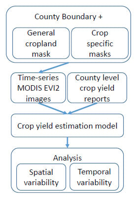
2. Materials and Methods

2.1. Study Area

The study area covers 28 counties in the Southern, Western, and Central Ontario regions, excluding Haliburton, Muskoka, and Parry Sound, the three counties with minor cropping activities (Figure 1). It is within the Mixedwood Plains Ecozone, a primary agricultural region at the most southern part of Canada. The area is characterized by warm to hot summers and cold winters, fertile soils, and adequate water supply for agricultural production [32]. Dominant crops are soybean (~2 Mha), grain corn (~1.5 Mha), and winter wheat (~0.9 Mha), rotated with perennial forage crops (~1.5 Mha including hay and pasture), varying from year to year. Over the past 15 years, more than 82% of corn, 85% of soybean, 90% of winter wheat, and about 65% of forage crops in Ontario were grown in these three regions. The four crops have different phenological patterns. Winter wheat is seeded in the previous fall, survives the cold winter with very slow growth, and grows fast in the following spring. The canopy reaches full coverage in late spring and becomes physiological mature and is harvested in late July to early August. Soybean and corn are seeded in May and harvested between late September and early November. Forage crops start to grow and the canopy reaches full ground coverage quickly in spring, and are then harvested (or grazed) multiple times during the growing season, and go dormant in winter. Typical growth calendars for these crops can be found in Liu et al. [31] and Huffman et al. [30].

2.2. Crop Data

Reported crop grain yield and harvested area of the three annual crops at county level were obtained from the Ontario Ministry of Agriculture, Food and Rural Affairs (OMAFRA; http://www.omafra.gov.on.ca/english/) for the 14 year period from 2003 to 2016. In all the counties in Southern Ontario, the largest proportion of area was planted with soybean, and the smallest proportion of area was planted with forage crops. In central Ontario, the largest proportion of area was planted with forage crops. Areas of different crops were relatively balanced in Western Ontario. Average yields for all the counties over the 14 year period were 8.84 t ha-1 for corn, 4.88 t ha-1 for winter wheat, and 2.71 t ha-1 for soybean. An increasing trend of about 0.16 t ha-1 year-1 for corn, 0.06 t ha-1 year-1 for winter wheat, and 0.05 t ha-1 year-1 for soybean was observed during this time period. Correlation between county-level yields of the crops over the 14 years was statistically significant. More specifically, the correlation between the yields of corn and soybean (R2 = 0.71, n = 378) was much stronger than the correlation between the yields of corn and wheat (R2 = 0.30, n = 377). Coefficient of variation of county-level crop yields over the period was between 7% and 17% for corn, 6% and 25% for soybean, and 10% and 21% for winter wheat. The reported county-level yields were used to assess the capability of MODIS data for yield estimation, and the county-level harvested areas were used to assess the crop classification.

2.3. Time-Series MODIS Data Processing

MODIS 250 m 8 day composite reflectance product (MOD09Q1, version 5) from 2003 to 2016, and the 500 m land cover type products (MCD12Q1) from 2000 to 2014, were obtained from the Land Processes Distributed Active Archive Center (LP DAAC). The study area is completely covered by two MODIS tiles, h11v04 and h12v04. MODIS tiles were mosaicked using the MODIS re-projection tool (MRT). There were 46 reflectance composites each year. The 250 m reflectance product allows for calculation of vegetation indices with a higher temporal resolution than the standard vegetation index product MOD13Q1.

2.3.1. Calculation of the Two-Band Enhanced Vegetation Index (EVI2)

Instead of NDVI, the two-band enhanced vegetation index (EVI2; [33]) was used in this study for crop yield estimation, as it is less susceptible to saturation at high biomass [33,34,35], which is the case in the study region. Son et al. [36] reported that EVI2 performed slightly better than NDVI for yield estimation. EVI2 can be calculated from the red ( ρ R ) and near infrared ( ρ N ) band reflectance as is shown below:
E V I 2 = 2.5 ( ρ N ρ R ) / ( ρ N + 2.4 ρ R + 1 ) .

2.3.2. Crop Masks

Crop masks could be generated using crop classification maps; however, annual crop inventory maps in Canada became operational only after 2011. In this study, cropland masks were generated from the MODIS land cover product, and classification of the time-series reflectance data was conducted using a fuzzy decision tree algorithm [31]. Firstly, a general cropland mask was generated by merging classification codes 12 (cropland) and 14 (cropland/natural vegetation mosaic) in the land cover type-1 classifications in the MCD12Q1 product. A pixel was included in the cropland mask if it was classified as class 12 or class 14 in any of the years between 2000 and 2014. The data were then resampled from 500 m into 250 m resolution using the nearest neighbor method to match that of the reflectance data. Secondly, the TIMESAT software package [37,38] was used to model the time-series EVI2 using logistic functions, from which several phenological indicators characterizing the shape of the seasonal growth curves were defined, such as the maximum EVI2, the time when peak EVI2 (85% of the maximum) started and ended, and the time span when EVI2 was larger than 60% peak level. Thirdly, a fuzzy decision tree classifier based on the phenological indicators was developed to identify the major crop types in this region—corn, soybean, winter wheat, and forage. The classifier was trained using 30 m high resolution annual crop inventory map of 2013 [39], resampled to the pixel size of the MODIS products, and tested using crop inventory maps for 2011 and 2012. The accuracies for the two tested years were comparable with the accuracy of the training year, with an overall accuracy about 75%. Detailed information on the classification algorithm and results are reported in Liu et al. [31]. The classifier was applied to identify pure pixels of the major crop types annually between 2003 and 2016, and annual crop-specific masks were derived for MODIS data extraction.

2.3.3. Extraction of County Level Average EVI2

County level average time-series EVI2 was extracted using the general cropland mask and crop-specific masks for yield estimation. MODIS data were only extracted from pixels with good quality according to the quality attributes associated with the MODIS product, that is, pixels that were clear or assumed clear of cloud contamination, and were not in cloud shadow.

2.4. Modeling for Yield Estimation

Regression analysis was conducted between county-level crop yields and MODIS EVI2 to study the explanatory capability of time-series EVI2 for mapping regional yield variability. A linear model was used because vegetation indices are considered to be linearly related to crop photosynthetic capacity [40,41], which can be used to model crop biomass accumulation and yield [13,28,42,43]. In our earlier study, NDVI was correlated with crop yields to investigate its capability for county level yield estimation [44]. In this study, linear correlation analysis was conducted between crop yields and EVI2 for all years combined (all-year model) and for each year individually (year-specific) in three agricultural regions separately. For the all-year model, year was treated as an additional variable to account for the long term trends of yields, thus a multiple linear regression model was adopted:
Y = a 0 + a 1 E V I 2 +   a 2   A
where Y is county level yield; EVI2 represents county level average derived with a crop mask for a given time in the growing season; A is the year; and a 0 , a 1 , and a 2 are regression coefficients. Although an all-year model was desirable, we conducted a year-specific regression to investigate the inter-annual variability of the relationships between crop yields and EVI2.
The coefficient of determination (R2)—also defined as the Nash–Sutcliffe model efficiency coefficient—the root mean square error (RMSE), and the mean relative absolute error (MRAE) were calculated to assess the correlation between yield and EVI2 and the performance of the regression models:
R 2 = 1 i = 1 n ( Y i o Y i e ) 2 / i = 1 n ( Y i o Y ¯ o ) 2 ,
RMSE = i = 1 n ( Y i o Y i e ) 2 / n ,
MRAE = ( i = 1 n | Y i o Y i e | / Y i o ) / n ,
where Y represents yield, o indicates reported yields and e indicates estimated yields, i represents an individual sample (of a county in a year), and n is the total number of samples. Relative RMSE (RRMSE) was calculated as percentage to the mean crop yields.

3. Results

3.1. Crop Classification

To assess the performance of crop identification using the fuzzy decision tree algorithm, area proportions of the four major crops estimated from the classification were compared with those reported by OMAFRA at the county level for all 14 years (Figure 2). Area proportions were calculated on the basis of the total areas of the four major crops because only these four crops were identified in the study area. Given that the four crops constitute more than 85% of the total crop area in the region, we consider the results acceptable, although the approximation could induce bias.
For most counties, the proportions of winter wheat area were around 13%, and could approach 30% in some counties (Figure 2a). There was a large overestimation of winter wheat in many counties. Identification of corn was better, although discrepancy was still observed (Figure 2b). There was a persistent underestimation of soybean due to a large omission error in classification (Figure 2c). Estimated area proportions of forage crops correlated well with the reported proportions; however, overestimation was also observed for most of the counties (Figure 2d). As reported by Liu et al. [1], there was large confusion between winter wheat and forage crops, and between corn and soybean in the classification. The phenological patterns of soybean and corn were similar, with only a slightly shorter peak growth duration for soybean. Winter wheat and forage crops also have a similar pattern with a quick and early growth phase in early spring, and undergo a complicated procedure in summer, either due to mechanical harvest and then volunteer regrowth for forage crops, or harvest of winter wheat followed by reseeding with cover crops to protect soil in winter [30]. These factors bring additional challenges for crop identification using coarse resolution satellite data such as MODIS imagery. Figure 2e, f shows the comparison of the two pairs of crops combined. Areal proportions for corn and soybean combined were mostly underestimated in most cases, and forage and winter wheat were mostly overestimated.
Classification results can also be assessed using average seasonal growth profiles of the three annual crops represented by time-series EVI2. Figure 3a–c shows growth curves of winter wheat, corn, and soybean in three counties, Chatham-Kent in Southern Ontario, Perth County in Western Ontario, and Durham in Central Ontario, as examples. The growth profiles were constructed using extracted EVI2 from “pure” pixels identified by the classification algorithms for the three crops in 2016. Growth profiles extracted using a general cropland mask for the three counties are shown in Figure 3d. It was observed that EVI2 of winter wheat reached peak stage from late May to early June, and declined to minimum at the end of July when the crop is senescent and ready for harvest. Corn and soybean started to grow from late May, reaching peak growth status between late July and end of August. Because most areas in these three counties were seeded with soybean and corn combined, seasonal vegetation growth profiles extracted using a general cropland mask showed a typical pattern of the two summer crops (Figure 3d), that is, reach peak stage in late July. In 2016, the area seeded with corn and soybean was about 80% in Chatham-Kent, whereas only about 60% in Perth and Durham. Another factor causing the discrepancy could be associated with variability of phenological cycles pertaining to different crop varieties that could not be specified in this study.
In summary, although the estimated areal proportions obtained from the classification algorithm had a large discrepancy with the reported area proportions, the growth curves of the three annual crops reflected their typical phenological patterns with contamination by other crops.

3.2. Seasonal Variation of Linear Correlation Between EVI2 and Crop Yields

A multiple linear regression (Equation (2)) was conducted using crop yields from all the 14 years (2003 to 2016) and in all the counties combined, and using EVI2 extracted with a general cropland mask (GM), and crop-specific masks (SM) derived from classification. The intention was to explore the general explanatory power of EVI2 as a function of time across a typical growing season. The correlation coefficients are shown in Figure 4 for the three crops. This allows for discrimination of positive versus negative correlations. A clear seasonal pattern can be observed for all cases. EVI2 derived using a general cropland mask had a negative correlation with the yields of the three annual crops during a period around the end of May (day-of-year (DOY) = 150) and the end of October (DOY = 300), and a positive correlation during a period around the end of July (DOY = 210) corresponding to the peak growth stage of corn and soybean, the two dominant crops in the region. The transition from negative to positive correlations for the three crops occurred between the end of June and the start of July. Using crop-specific masks, the strongest positive correlation for winter wheat changed to mid-to-late May, whereas the time of the strongest positive correlation did not change for corn and soybean. When crop specific masks were used, the strongest positive correlation occurred approximately at peak growth stages of respective crops, that is, late May for winter wheat and late July and early August for corn and soybean. This was because vegetation indices at the peak stage captured the variability of maximum green biomass accumulation up to this stage, which was largely carried over to the variability of final yields. The negative correlation between the yields of corn (and soybean) and EVI2 at around the end of May and end of October was reduced when crop specific masks were used.

3.3. Inter-Annual Variability of the Linear Relationships

Linear regression was conducted for each year between county level yields and time-series EVI2 extracted using the two types of cropland masks. The results for the strongest correlations are shown in Figure 5, which include relative root mean square error (RRMSE, %), coefficient of determination R2, and mean relative absolute error (MRAE) (%). Annual averages of county level yields and the coefficient of variation (CV) (%) are also shown in Figure 5.
For winter wheat (Figure 5a,d), county level annual yield variability—represented by CV—was between 10% and 21% during the 14 year period. Except for 2011 using the general cropland mask and 2012 using crop specific mask, the strongest linear correlation between yields and EVI2 was significant at the 5% level (n = 27). The correlations between yields and EVI2 showed a strong inter-annual variation, as represented by both MRAE and DOY, at which the strongest correlation was observed. DOY of the strongest positive correlation ranged between 193 (mid-July) and 241 (end of August) when the general cropland mask was used, and ranged between DOY 121 (early May) and 169 (mid-June) when crop-specific mask was used. MRAE was larger than 10% for a few years and in most cases ranged between 7% and 9%.
For corn (Figure 5b,e), CV of county level yields ranged between 7% and 17%. Correlation between yields and EVI2 was significant (n = 26) for all cases. DOY of the largest R2 was between 193 (mid-July) and 257 (mid-September), but mostly in late July and early August. DOY for the two crop masks was about the same for most years but had large differences for some of the years. For instance, the best DOY was 241 using the general cropland mask and 201 using the crop-specific mask in 2006. MRAE was below 8% in most cases, and for some cases was as low as 3%, for example, in 2003 and 2011. MRAE was comparable using the two crop masks, although there was a slight tendency of a smaller MRAE using the general cropland mask.
For soybean (Figure 5c,f), CV of county level yields showed a larger inter-annual variation than the other two crops, ranging between 6% (in 2013) and 25% (in 2007). Correlation was significant at the 5% level (n = 25) for all years except for 2014 using the crop-specific mask (R2 = 0.07). Similar to that for corn, the time window best for soybean yield estimation was between mid-July and late August. Although estimation error remained relatively low in most cases (MRAE < 7%), a large difference in the best DOY within a time window of about 40 days after late July (DOY = 193) was also observed.
To illustrate the inter-annual variation of the relationships between crop yields and EVI2, scatter-plots between reported crop yields and EVI2 were shown in Figure 6 for 3 years (2006, 2011, and 2016) as examples. EVI2 was extracted using the crop-specific masks from the time with strongest correlation for winter wheat, corn, and soybean, respectively. Inter-annual variability of the relationships between crop yields and EVI2 was remarkable, both in terms of best time for the prediction and the regression models. For winter wheat, the range of yields was much wider in 2011 and 2016 than in 2006, with CV of 21%, 18%, and 13%, respectively. The relationships were quite different for the 3 years. Correlation was the strongest in 2006 with the smallest MRAE (5%) using MODIS 8-day composite at DOY = 137 (mid-May). Samples for 2016 had the lowest EVI2 because the data was from composite DOY = 121, about 2 weeks earlier than that for the other 2 years. For corn, the range of county yields was smaller in 2006 and 2011 than in 2016. Although the best time for yield prediction was separated by about 3 weeks (DOY = 201 in 2006 and 225 in 2011), regression equations for the 2 years were similar. Again, EVI2 in 2016 was lower because MODIS data were from composites at the end of August, corresponding to the senescent stage. For soybean, a narrower dynamic range of yield was also observed in 2006 and 2011 compared with 2016; however, samples largely converged for all 3 years.

3.4. Yield Estimation Using a Multiple Linear Regression Model

A multiple linear regression model was established for county-level crop yield estimation using EVI2 and year as two independent variables. Results from previous sections show that the strongest correlation between crop yields and EVI2 were observed at the peak growth stages of the crops, with inter-annual variations of the best time within a time window. To establish a simple model applicable across different years, average EVI2 was derived within a narrow time window correspondent to the peak growth stages of the crops. The use of the average EVI2 for crop yield estimation will induce a loss of accuracy in some years, but can increase model robustness through a reduced variability associated with crop growth calendars. The time window for averaging was from DOY 201 to 217 using the general cropland mask, from DOY 121 to 145 using crop-specific mask for winter wheat, and from DOY 209 to 241 for corn and soybean using the two masks. In considering that cropping practices (cultivars and growth calendars) might be different among the three agricultural regions (Southern, Western, and Central Ontario), the regression model was established individually for each region. Performance was assessed on the results obtained using the three models independently, and on the results combined. Regression results and statistical performance indicators are reported in Table 1. Figure 7 shows the comparison between all the reported and estimated yields using general cropland mask and crop-specific masks. The following observations can be made:
(1) Crop yields can be estimated reliably in all cases using the multiple linear regression model (p < 0.001), except for winter wheat in Central Ontario, which had a low R2 (~0.10) and smaller F-value (p < 0.025). The inferior performance for winter wheat in Central Ontario was also demonstrated by a smaller correlation coefficient for EVI2 (r_EVI2; 0.03 for SM and -0.06 for GM), and a larger uncertainty of the regression coefficients ( σ ( a 1 ) ) respective to the coefficient itself ( a 1 ). The regression coefficient for EVI2 was 0.909 ± 1.745 using crop-specific mask and -1.611 ± 1.539 using the general cropland mask. Trend of yields was the main factor of yield variability in this case (r_Year ~ 0.30).
(2) Performance of yield estimation was always poorer in Central Ontario than in the other two regions, as shown by a relatively larger MRAE and a lower R2.
(3) Models based on crop-specific masks achieved slightly better results than those based on a general cropland mask, according to MRAE and lower R2.
(4) Yields of the three crops had a clear increasing trend over the 14 year period, as shown by the positive correlation coefficients between crop yields and the year (r_Year in Table 1). Partial t-test showed that regression coefficient a 2 was at the significance level of p < 0.001 (t > 3.0). According to the derived coefficient a 2 , annual increase of crop yields was between 0.125 to 0.166 t/ha for corn, 0.037 to 0.058 t/ha for soybean, and 0.054 to 0.094 t/ha for winter wheat over the 14 year period, dependent on regions.
(5) Although EVI2 at peak growth stage accounted for yield variability effectively (Section 3.3), considerable temporal variability over the long period was due to the long term yield trends. Over the study period, yield variability due to the long term trend and due to spatial heterogeneity were comparable, as demonstrated by the comparable correlation coefficients r_EVI2 and r_Year.
(6) For all cases in Figure 7, there was an underestimation when yields were higher than average and an overestimation when yields were lower than average. This tendency was less severe when crop-specific masks were used, as linear regression between the estimated and reported yields had a larger slope using crop-specific masks than using a general cropland mask.

4. Discussion

4.1. Discrimination of Major Crops

For crop yield estimation using vegetation indices, the index should represent a particular crop. Annual crop inventory map was not available before the year of 2011 in Canada, making it difficult to estimate yields in a historical year. Using the cloud computing platform of the Google Earth Engine, Massey et al. [45] produced high-resolution (30 m) circa-2010 cropland extent classification for North America; however, different crops were not identified. Using annual crop classification maps of multiple years, crop-specific masks were generated and used for yield forecast in Canada [46]; however, the masks represent spatio-temporal “likelihood” distribution of crops and do not reflect the annual variation of the crop area changes. Using the decision tree algorithm, we were able to discriminate the four major crops with minimal requirement of ground truth data for training the classifier, thus mapping major crop types back to 2000 using 250 m time-series MODIS data [31]. Although a satisfactory result was achieved to extract “pure” crop pixels, the majority of pixels at 250 m resolution were mixed in the regions of study, leading to large omission/commission errors in classification and impacting the creation of crop-specific masks (Figure 2). County-level phenological patterns for the three annual crops, represented by EVI2 extracted using crop-specific masks, were contaminated by this pixel mixing effect (Figure 3). Many experimental studies have been conducted to merge high-spatial-low-temporal resolution data with low-spatial-high-temporal resolution data to generate time-series high resolution data [17,27,28,29,47]. Although applying this approach to the regional scale can be a challenge due to huge data volume and the need for intensive computational resources, it could be applicable as cloud computing becomes mature, or if the approach could be implemented at field scale instead of pixel scale.

4.2. Issues with Crop Yield Estimation in Areas with Mixed Cropping System

It is observed that EVI2 extracted using the general cropland mask was correlated with yields of the three annual crops positively in summer and negatively in spring and fall. This reveals the following two aspects of the reality. First, yields of the three crops were highly correlated, with a much stronger correlation between corn and soybean (R2 = 0.71) than that between corn and winter wheat (R2 = 0.30). This echoes similar yield limiting factors of the three crops related to environmental conditions. The relatively weaker correlation between winter wheat and the two summer crops could be due to the difference in their growing cycles and the experienced different meteorological conditions. In the study region, the peak growth stage for winter wheat is in late May, whereas for corn and soybean it is in August. Second, the negative correlation in spring could be due to the typical phenological cycles and the area proportion of soybean and corn. A negative correlation was observed between county-level EVI2 during the spring and the areal proportions of corn and soybean (Figure 8a). This was understandable because these two crops are seeded in spring when the corresponding EVI2 is low; thus, the larger areal proportion of these two crops corresponded to the lower average EVI2. On the contrary, the county-level areal proportion of these two crops was positively correlated with the county level grain yield (Figure 8b). This suggests that soybean and corn are less likely to be seeded in counties where yield of the two crops is low. According to the reported crop yields and harvested areas, the counties distributed to the east and north of the study area have relatively lower yields, and this tendency is persistent from year to year. The negative correlation indicates that the effect associated with area proportions of different crops has not been completely eliminated by using crop-specific masks (Figure 4).
The inferior performance for yield estimation in Central Ontario (larger MRAE) was because crop yields in this region are relatively low. Another reason is that annual crops are not extensively distributed in the region, thus coarse resolution MODIS EVI2 cannot effectively capture annual crop growth conditions. Higher resolution remote sensing data would be useful in improving the performance in this case.
As shown in Figure 2, large confusion existed between classification of corn and soybean and between winter wheat and hay, but not between the two groups. This confusion would not have a big impact on yield estimation from EVI2 at peak growing stage extracted using the crop-specific masks, as during their peak growing stages, corn and soybean had about the same EVI2, and winter wheat and hay had about the same EVI2. Further improvement of crop-specific masks might improve yield estimation, but this will rely on higher resolution data to reduce pixel mixing effects.

4.3. Issues with Yield Estimation across Different Years

The goal of this study was to establish a crop yield estimation model applicable across different years for regions with mixed crops using MODIS vegetation indices. The long-term crop yield increasing trend has not been considered in some of the similar yield estimation models [1,21,42]. Using a regression tree approach, Johnson estimated corn and soybean yields from MODIS NDVI and the daytime land surface temperature (LST) in the United States corn belt region [1]. The estimation error for the years 2006–2011 was 0.38–0.47 t/ha for soybean and 0.96–1.26 t/ha for corn. Taking into consideration the yield trends, we obtained an estimation error of 0.29–0.32 t/ha for soybean and 0.74–0.87 for corn using peak growing stage EVI2 only. Using a simple linear regression and phenologically adjusted MODIS EVI2, Bolton and Friedl estimated crop yields in Central United States [42], and obtained a relative estimation error of 8%–14% for soybean and 9%–12% for corn in the years 2004–2009. In our study, the estimation error using crop-specific masks was 9.7% for soybean and 7.3% for corn. This shows the effectiveness of our model for crop yield estimation.
Although the established multiple linear regression models performed well for yield estimation of the three crops across different years, large estimation error can happen in some years. Figure 9 shows the comparison of MRAE for yield estimation, obtained using the all-year multiple linear regression models and using the year-specific strongest linear regression models based on time-series EVI2 only. Each sample represents estimation error for one year. The samples reside mostly below the 1:1 lines, showing a lower estimation accuracy using the all-year model.
For winter wheat, the difference between the all-year model and the year-specific model was relatively small. The largest difference was in 2016 for the models using the general cropland mask, with MRAE of 16% for the all-year model and 10% for the year-specific model, and respective MRAE of 11% and 13% for the models using crop-specific mask (Figure 9a). For corn, the largest difference was observed in 2004, with MRAE of 14% using crop specific mask, 12% using the general cropland mask for the all-year model, and 4% for the year-specific model (Figure 9b). For soybean, the largest difference was observed in 2004 (15% and 16% using the all-year model, and 6% and 7% using year-specific model, for general cropland mask and crop-specific mask, respectively) and 2007 (24% and 20% using the all-year model, and 7% and 11% using the year-specific model, for general cropland mask and crop-specific mask, respectively) (Figure 9c). This large difference in estimation errors between the all-year model and the year-specific model might have been induced by a lower than normal precipitation in the maturity stage of the two crops (in September). Figure 10 shows the monthly precipitation during July–September versus the long term monthly precipitation normal, as obtained from the weather station in London, Ontario. The monthly precipitation in September of 2004 (18.4 mm) and 2007 (44.6 mm) was much lower than normal (98.9 mm), which may have impacted crop growth after the peak stage in August, which had not been captured by peak growing stage EVI2.
It was considered that the year-specific model captured the spatial variability of yields, whereas the all-year model captured both spatial and temporal variability. It then seems that spatial variability of corn and soybean yields were captured by EVI2 better than that of winter wheat, as demonstrated by a generally lower MRAE using the year-specific model. In contrast, the all-year models showed an inefficiency in capturing inter-annual variability of corn and soybean yields for some years (Figure 9b,c). For the all-year model, the variable “year” captured temporal variability only, by assuming a constant variation of yields throughout the whole period, yet this might not be true. The average EVI2 at peak growth stages captured spatial variability as well as temporal variability if inter-annual variability of growth conditions showed up during the peak growth stages. A limit for the model in this study was that yield variability induced by abnormal growth conditions after the peak growth stage was not captured.

4.4. Inter-Annual Variability of the Relationships between EVI2 and Crop Yields

Vegetation indices are highly correlated with crop photosynthetic capacity [10,48], and can be used to model biomass accumulation and to estimate crop yield [13,49]. They are standard products (or can be derived) from measurements of many satellite sensors, particularly for the coarse resolution operational satellites [50,51,52,53]. This provides a basis for regional-scale crop yield modeling using regression models [1,21,42]. It was observed that crop yield was best correlated with EVI2 derived from a time period corresponding to peak growth stage of the crops (Figure 3 and Figure 4), which has been confirmed by many studies. For instance, it was reported that MODIS data acquired 65–75 days after green-up for maize and 80 days after green-up for soybean provided the best yield forecast in Central United States [42]. Mkhabela et al. [21] observed that MODIS NDVI from late June to early July can provide preliminary yield forecasts across the Canadian Prairies. The study by Johnson [1] on soybean and corn yield estimation in the corn belt region of the central United States also showed that MODIS NDVI was best from late July to early August.
However, empirical models based on vegetation indices may be spatially or temporally dependent [19]. The inter-annual variability was shown by either variations of the best time for yield estimation or the difference in linear regression models (Figure 5). This was determined by year-specific meteorological conditions, crop growth calendars, as well as management practices (e.g., areal proportions of crops and rotational decisions). EVI2 at peak growth stage can capture the cumulative growth conditions before this time but cannot capture important yield limiting events onwards. As observed from this study, the exact time for the highest R2 between yield and EVI2 varied within a wide time window, in which the linear correlation was still significant but was lower than the largest R2. A regression model could be established by averaging vegetation indices over this time window [21,54]. This would lead to a more stable regression model applicable to multiple years and might be useful for yield forecasting, but will induce an inferior performance for a particular year when specific yield limiting events in that year are not captured.

5. Conclusions

In this study, time-series two-band enhanced vegetation index (EVI2) derived from 8 day composite 250 m MODIS reflectance data were used for crop yield estimation at the county level in Southern, Western, and Central Ontario agricultural regions. The regions are characterized by major crops of distinct phenological patterns, such as winter wheat and forage crops versus soybean and corn. A fuzzy decision tree classifier was used to identify these major annual crops to create crop-specific masks for extraction of county-level EVI2. The classification algorithm was able to identify pure pixels of major crops in the study area, with relatively large errors compared with high resolution crop classification maps and the reported county-level harvested area of crops. County-level crop yields were strongly correlated with EVI2 extracted at peak crop growth stages. Crop-specific masks were found to be able to decompose the compounding effects of different phenological patterns. Although accuracy of crop yield estimation using a general cropland mask was not considerably lower than that using crop-specific masks, the model may be impacted by other factors such as areal proportions of different crops. Cautions should be taken in using the general cropland mask when actual cropping condition (e.g., difference in relative areal proportions) is not known. The multiple linear regression model using peak stage average EVI2 and the year as independent variables can be used to map spatial-temporal variability of crop yields across different years with satisfaction; however, model performance may be poor in some years when important yield limiting factors are not captured by EVI2 at the peak growth stage. Further refinement of crop-specific masks and incorporation of additional information on growth conditions may help improve the performance of crop yield estimation at regional scale.

Author Contributions

Conceptualization, J.L., J.S., B.Q., and T.H.; data curation, J.L.; formal analysis, J.L.; funding acquisition, J.S., B.Q., T.H., and T.M.; investigation, J.L.; methodology, J.L., B.Q., and Y.Z.; project administration, J.S. and T.H.; resources, J.S.; validation, J.L., T.D., and Q.J.; writing—original draft, J.L.; writing—review and editing, B.Q., J.S., T.H., Y.Z., T.D., Q.J., and T.M.

Funding

This study was supported by Agriculture and Agri-Food Canada (AAFC) under the Sustainability Metrics project (#J-000486), the Bio-products Targeted Call project (#J-001598), and the Integrated Soil and Land Use data project (#J-001383).

Conflicts of Interest

The authors declare no conflict of interest.

References

  1. Johnson, D.M. An assessment of pre- and within-season remotely sensed variables for forecasting corn and soybean yields in the united states. Remote Sens. Environ. 2014, 141, 116–128. [Google Scholar] [CrossRef]
  2. Drury, C.F.; Yang, J.; DeJong, R.; Huffman, E.C.; Reid, K.; Yang, X.M.; Bittman, S.; Desjardins, R.L. Residual soil nitrogen indicator. In Environmental Sustainability of Canadian Agriculture: Agri-Environmental Indicator Report Series—Report #4; Clearwater, R.L., Martin, T., Hoppe, T., Eds.; Agriculture and Agri-Food Canada: Ottawa, ON, Canada, 2016; pp. 115–120. [Google Scholar]
  3. Huffman, T.; Liu, J. Soil cover. In Environmental Sustainability of Canadian Agriculture: Agri-Environmental Indicator Report Series—Report #4; Clearwater, R.L., Martin, T., Hoppe, T., Eds.; Agriculture and Agri-Food Canada: Ottawa, ON, Canada, 2016; pp. 53–63. [Google Scholar]
  4. Liu, J.; Huffman, T.; Green, M. Potential impacts of agricultural land use on soil cover in response to bioenergy production in canada. Land Use Policy 2018, 75, 33–42. [Google Scholar] [CrossRef]
  5. Desjardins, R.L.; Worth, D.E.; Verge, X.; Maxime, D.; VanderZaag, A.C.; Dyer, J.A.; Arcand, Y. Greenhouse gas emission intensities of agricultural products. In Environmental Sustainability of Canadian Agriculture: Agri-Environmental Indicator Report Series—Report #4; Clearwater, R.L., Martin, T., Hoppe, T., Eds.; Agriculture and Agri-Food Canada: Ottawa, ON, Canada, 2016; pp. 211–222. [Google Scholar]
  6. Balaghi, R.; Tychon, B.; Eerens, H.; Jlibene, M. Empirical regression models using ndvi, rainfall and temperature data for the early prediction of wheat grain yields in morocco. Int. J. Appl. Earth Obs. Geoinf. 2008, 10, 438–452. [Google Scholar] [CrossRef]
  7. Wall, L.; Larocque, D.; Léger, P.-M. The early explanatory power of ndvi in crop yield modelling. Int. J. Remote Sens. 2008, 29, 2211–2225. [Google Scholar] [CrossRef]
  8. Prasad, A.K.; Chai, L.; Singh, R.P.; Kafatos, M. Crop yield estimation model for iowa using remote sensing and surface parameters. Int. J. Appl. Earth Obs. Geoinf. 2006, 8, 26–33. [Google Scholar] [CrossRef]
  9. Asner, G.P. Biophysical and biochemical sources of variability in canopy reflectance. Remote Sens. Environ. 1998, 64, 234–253. [Google Scholar] [CrossRef]
  10. Myneni, R.B.; Williams, D.L. On the relationship between fapar and ndvi. Remote Sens. Environ. 1994, 49, 200–211. [Google Scholar] [CrossRef]
  11. Viña, A.; Gitelson, A.A. New developments in the remote estimation of the fraction of absorbed photosynthetically active radiation in crops. Geophys. Res. Lett. 2005, 32. [Google Scholar] [CrossRef]
  12. Hatfield, J.L. Radiation use efficiency: Evaluation of cropping and management systems. Agron. J. 2014, 106, 1820–1827. [Google Scholar] [CrossRef]
  13. Liu, J.; Pattey, E.; Miller, J.R.; McNairn, H.; Smith, A.; Hu, B. Estimating crop stresses, aboveground dry biomass and yield of corn using multi-temporal optical data combined with a radiation use efficiency model. Remote Sens. Environ. 2010, 114, 1167–1177. [Google Scholar] [CrossRef]
  14. Jégo, G.; Pattey, E.; Liu, J. Using leaf area index, retrieved from optical imagery, in the stics crop model for predicting yield and biomass of field crops. Field Crop. Res. 2012, 131, 63–74. [Google Scholar] [CrossRef]
  15. Jégo, G.; Pattey, E.; Mesbah, M.; Liu, J.; Duchesne, I. Impact of the spatial resolution of climatic data and soil physical properties on regional corn yield predictions using the stics crop model. Int. J. Appl. Earth Obs. Geoinf. 2015, 41, 11–22. [Google Scholar] [CrossRef]
  16. Fang, H.; Liang, S.; Hoogenboom, G.; Teasdale, J.; Cavigelli, M. Corn-yield estimation through assimilation of remotely sensed data into the csm-ceres-maize model. Int. J. Remote Sens. 2008, 29, 3011–3032. [Google Scholar] [CrossRef]
  17. Dong, T.; Liu, J.; Qian, B.; Zhao, T.; Jing, Q.; Geng, X.; Wang, J.; Shang, J.; Huffman, T. Estimating winter wheat biomass by assimilating leaf area index derived from fusion of landsat-8 and modis data. Int. J. Appl. Earth Obs. Geoinf. 2016, 49, 63–74. [Google Scholar] [CrossRef]
  18. Wiegand, C.L.; Richardson, A.J.; Jackson, R.D.; Pinter, P.J., Jr.; Aase, J.K.; Smika, D.E.; Lautenschlager, L.F.; McMurtrey, J.E., III. Development of agrometeorologlcal crop model inputs from remotely sensed information. IEEE Trans. Geosci. Remote Sens. 1986, 24, 90–98. [Google Scholar] [CrossRef]
  19. Doraiswamy, P.C.; Hatfield, J.L.; Jackson, T.J.; Akhmedoc, B.; Prueger, J.; Stern, A. Crop condition and yield simulations using landsat and modis. Remote Sens. Environ. 2004, 92, 548–559. [Google Scholar] [CrossRef]
  20. Funk, C.; Budde, M.E. Phenologically-tuned modis ndvi-based production anomaly estimates for zimbabwe. Remote Sens. Environ. 2009, 113, 115–125. [Google Scholar] [CrossRef]
  21. Mkhabela, M.S.; Bullock, P.; Raj, S.; Wang, S.; Yang, Y. Crop yield forecasting on the canadian prairies using modis ndvi data. Agric. For. Meteorol. 2011, 151, 385–393. [Google Scholar] [CrossRef]
  22. Shanahan, J.F.; Schepers, J.S.; Francis, D.D.; Varvel, G.E.; Wilhelm, W.W.; Tringe, J.M.; Schlemmer, M.R.; Major, D.J. Use of remote-sensing imagery to estimate corn grain yield. Agron. J. 2001, 93, 583–589. [Google Scholar] [CrossRef]
  23. Benedetti, R.; Rossini, P. On the use of ndvi profiles as a tool for agricultural statistics: The case study of wheat yield estimate and forecast in emilia romagna. Remote Sens. Environ. 1993, 45, 311–326. [Google Scholar] [CrossRef]
  24. Chipanshi, A.; Zhang, Y.; Kouadio, L.; Newlands, N.; Davidson, A.; Hill, H.; Warren, R.; Qian, B.; Daneshfar, B.; Bedard, F.; et al. Evaluation of the integrated canadian crop yield forecaster (iccyf) model for in-season prediction of crop yield across the canadian agricultural landscape. Agric. For. Meteorol. 2015, 206, 137–150. [Google Scholar] [CrossRef]
  25. Rasmussen, M.S. Operational yield forecast using avhrr ndvi data: Reduction of environmental and inter-annual variability. Int. J. Remote Sens. 1997, 18, 1059–1077. [Google Scholar] [CrossRef]
  26. Rasmussen, M.S. Developing simple, operational, consistent ndvi-vegetation models by applying environmental and climatic information. Part II: Crop yield assessment. Int. J. Remote Sens. 1998, 19, 119–139. [Google Scholar] [CrossRef]
  27. Feng, G.; Masek, J.; Schwaller, M.; Hall, F. On the blending of the landsat and modis surface reflectance: Predicting daily landsat surface reflectance. IEEE Trans. Geosci. Remote Sens. 2006, 44, 2207–2218. [Google Scholar] [CrossRef]
  28. Gao, F.; Anderson, M.; Daughtry, C.; Johnson, D. Assessing the variability of corn and soybean yields in central iowa using high spatiotemporal resolution multi-satellite imagery. Remote Sens. 2018, 10, 1489. [Google Scholar] [CrossRef]
  29. Liao, C.; Wang, J.; Pritchard, I.; Liu, J.; Shang, J. A spatio-temporal data fusion model for generating NDVI time series in heterogeneous regions. Remote Sens. 2017, 9, 1125. [Google Scholar] [CrossRef]
  30. Huffman, T.; Liu, J.; Green, M.; Coote, D.; Li, Z.; Liu, H.; Liu, T.; Zhang, X.; Du, Y. Improving and evaluating the soil cover indicator for agricultural land in canada. Ecol. Indic. 2015, 48, 272–281. [Google Scholar] [CrossRef]
  31. Liu, J.; Huffman, T.; Shang, J.; Qian, B.; Dong, T.; Zhang, Y. Identifying major crop types in eastern canada using a fuzzy decision tree classifier and phenological indicators derived from time series modis data. Can. J. Remote Sens. 2016, 42, 259–273. [Google Scholar] [CrossRef]
  32. Ecological Stratification Working Group (Canada). A National Ecological Framework for Canada; State of the Environment Directorate: Hull, QC, Canada, 1996.
  33. Jiang, Z.; Huete, A.; Didan, K.; Miura, T. Development of a two-band enhanced vegetation index without a blue band. Remote Sens. Environ. 2008, 112, 3833–3845. [Google Scholar] [CrossRef]
  34. Liu, J.; Pattey, E.; Jégo, G. Assessment of vegetation indices for regional crop green lai estimation from landsat images over multiple growing seasons. Remote Sens. Environ. 2012, 123, 347–358. [Google Scholar] [CrossRef]
  35. Shang, J.; Liu, J.; Huffman, T.; Qian, B.; Pattey, E.; Wang, J.; Zhao, T.; Geng, X.; Kroetsch, D.; Dong, T.; et al. Estimating plant area index for monitoring crop growth dynamics using landsat-8 and rapideye images. J. Appl. Remote Sens. 2014, 8, 085196. [Google Scholar] [CrossRef]
  36. Son, N.T.; Chen, C.F.; Chen, C.R.; Minh, V.Q.; Trung, N.H. A comparative analysis of multitemporal modis evi and NDVI data for large-scale rice yield estimation. Agric. For. Meteorol. 2014, 197, 52–64. [Google Scholar] [CrossRef]
  37. Eklundh, L.; Jönsson, P. Timesat 3.1 Software Manual; Lund University: Lund, Sweden, 2012; pp. 1–82. [Google Scholar]
  38. Jönsson, P.; Eklundh, L. Seasonality extraction by function fitting to time-series of satellite sensor data. IEEE Trans. Geosci. Remote Sens. 2002, 40, 1824–1832. [Google Scholar] [CrossRef]
  39. Davidson, A.M.; Fisette, T.; McNairn, H.; Daneshfar, B. Detailed crop mapping using remote sensing data (crop data layers). In Handbook on Remote Sensing for Agricultural Statistics (Chapter 4). Handbook of the Global Strategy to Improve Agricultural and Rural Statistics (GSARS); Delince, J., Ed.; GSARS: Rome, Italy, 2017. [Google Scholar]
  40. Roujean, J.L.; Breon, F.M. Estimating par absorbed by vegetation from bidirectional reflectance measurements. Remote Sens. Environ. 1995, 51, 375–384. [Google Scholar] [CrossRef]
  41. Vargas, L.A.; Andersen, M.N.; Jensen, C.R.; Joegrnsen, U. Estimation of leaf area index, light interception and biomass accumulation of miscanthus sinensis goliath from radiation measurements. Biomass Bioenergy 2002, 22, 1–14. [Google Scholar] [CrossRef]
  42. Bolton, D.K.; Friedl, M.A. Forecasting crop yield using remotely sensed vegetation indices and crop phenology metrics. Agric. For. Meteorol. 2013, 173, 74–84. [Google Scholar] [CrossRef]
  43. Pinter, P.J., Jr.; Jackson, R.D.; Idso, S.B.; Reginato, R.J. Multidate spectral reflectance as predictors of yield in water stressed wheat and barley. Int. J. Remote Sens. 1981, 2, 43–48. [Google Scholar] [CrossRef]
  44. Liu, J.; Huffman, T.; Shang, J.; Qian, B.; Dong, T.; Zhang, Y.; Jing, Q. Estimation of crop yield in regions with mixed crops using different cropland masks and time-series modis data. In Proceedings of the 2016 IEEE International Geoscience and Remote Sensing Symposium (IGARSS), Beijing, China, 10–15 July 2016; IEEE: Beijing, China, 2016; pp. 7161–7163. [Google Scholar]
  45. Massey, R.; Sankey, T.T.; Yadav, K.; Congalton, R.G.; Tilton, J.C. Integrating cloud-based workflows in continental-scale cropland extent classification. Remote Sens. Environ. 2018, 219, 162–179. [Google Scholar] [CrossRef]
  46. Zhang, Y.; Chipanshi, A.; Daneshfar, B.; Koiter, L.; Champagne, C.; Davidson, A.; Reichert, G.; Bedard, F. Effect of using crop specific masks on earth observation based crop yield forecasting across Canada. Remote Sens. Appl. Soc. Environ. 2019, 13, 121–137. [Google Scholar] [CrossRef]
  47. Huang, B.; Song, H. Spatiotemporal reflectance fusion via sparse representation. IEEE Trans. Geosci. Remote Sens. 2012, 50, 3707–3716. [Google Scholar] [CrossRef]
  48. Inoue, Y.; Penuelas, J.; Miyata, A.; Mano, M. Normalized difference spectral indices for estimating photosynthetic efficiency and capacity at a canopy scale derived from hyperspectral and CO2 flux measurements in rice. Remote Sens. Environ. 2008, 112, 156–172. [Google Scholar] [CrossRef]
  49. Li, Z.; Yu, G.; Xiao, X.; Li, Y.; Zhao, X.; Ren, C.; Zhang, L.; Fu, Y. Modeling gross primary production of alpine ecosystems in the tibetan plateau using modis images and climate data. Remote Sens. Environ. 2007, 107, 510–519. [Google Scholar] [CrossRef]
  50. Gobron, N.; Pinty, B.; Verstraete, M.; Govaerts, Y. The meris global vegetation index (MGVI): Description and preliminary application. Int. J. Remote Sens. 1999, 20, 1917–1927. [Google Scholar] [CrossRef]
  51. Huete, A.; Didan, K.; Miura, T.; Rodriguez, E.P.; Gao, X.; Ferreira, L.G. Overview of the radiometric and biophysical performance of the modis vegetation indices. Remote Sens. Environ. 2002, 83, 195–213. [Google Scholar] [CrossRef]
  52. Latifovic, R.; Trishchenko, A.P.; Chen, J.; Park, W.B.; Khlopenkov, K.V.; Fernandes, R.; Pouliot, D.; Ungureanu, C.; Luo, Y.; Wang, S.; et al. Generating historical AVHRR 1 km baseline satellite data records over canada suitable for climate change studies. Can. J. Remote Sens. 2005, 31, 324–348. [Google Scholar] [CrossRef]
  53. Wolters, E.; Swinnen, E.; Toté, C.; Sterckx, S. Spot-VGT Collection 3 Products User Manual, v1.2; Flemish Institute for Technological Research (VITO): Antwerp, Belgium, 2018. [Google Scholar]
  54. Hochheim, K.P.; Barber, D.G. Spring wheat yield estimation for western canada using NOAA NDVI data. Can. J. Remote Sens. 1998, 24, 17–27. [Google Scholar] [CrossRef]
Figure 1. Study area in Ontario, Canada. The dark lines outline the five regions in Ontario; the light gray polygons are counties included in the study, and the dark gray polygons are three counties representative of Southern (Chatham-Kent), Western (Perth), and Central (Durham) Ontario.
Remotesensing 11 02419 g001
Figure 2. Comparison of county level crop area proportions estimated annually using the fuzzy decision tree classifier and reported by the Ontario Ministry of Agriculture, Food and Rural Affairs (OMAFRA) for the period between 2003 and 2016.
Remotesensing 11 02419 g002
Figure 3. Crop growth profiles from March to October, illustrated using two-band enhanced vegetation index (EVI2) extracted for winter wheat (a), corn (b), soybean (c), and the three crops combined (d). The curves were derived from 2016 for three representative counties in Southern (Chathem-Kent), Western (Perth), and Central (Durham) Ontario (refer to Figure 1).
Remotesensing 11 02419 g003
Figure 4. Correlation coefficient between crop yield and EVI2 obtained through the multiple linear regression model, using data for all years (2003–2016). EVI2 was extracted using general cropland mask (GM) and crop-specific masks (SM).
Remotesensing 11 02419 g004
Figure 5. Annual variation of the strongest correlation between crop yields and time-series EVI2, extracted using a general cropland mask (GM) and crop-specific masks (SM) for winter wheat (a,d), corn (b,e), and soybean (c,f). Yield: average county level yield; R2: coefficient of determiantion; CV: coefficient of variation of yields; RRMSE: root mean square error relative to average yield; MRAE: mean relative absolute error. Samples from the three agricultural regions were analyzed together.
Remotesensing 11 02419 g005
Figure 6. Example annual relationships between crop yields and EVI2 derived using crop specific masks for the three annual crops; only data from 3 years (2006, 2011, and 2016) are shown; DOY refers to MODIS nominal composite day-of-year with the strongest correlation between EVI2 and crop yields.
Remotesensing 11 02419 g006aRemotesensing 11 02419 g006b
Figure 7. Relationships between reported and estimated crop yields at the county level for the period from 2003 to 2016. Crop yields were estimated using a multiple linear regression model from average EVI2 at the peak growth stages and year as independent variables. EVI2 was extracted using a general cropland mask (GM) and crop-specific masks (SM).
Remotesensing 11 02419 g007
Figure 8. Relationships of county level areal proportions of corn and soybean combined with (a) EVI2 at day-of-year (DOY) 153 and (b) corn yield.
Remotesensing 11 02419 g008
Figure 9. Comparison of yield estimation error, that is, mean relative absolute error (MRAE, %), using 250 m MODIS EVI2 using year-specific models and an all-year model. EVI2 was extracted using a general cropland mask and crop-specific mask for 2003–2016. The circles show the results of the years when there is a large difference between the all-year model and the year-specific model using the general cropland mask.
Remotesensing 11 02419 g009
Figure 10. Monthly precipitation for July–September from the weather station at London, Ontario (Station identifier: 6144475), versus correspondent long term normals from 1985 to 2016 shown with the same color but in dashed lines.
Remotesensing 11 02419 g010
Table 1. Models for yield estimation (Equation (2)) in three agricultural regions, and their performance assessment. a 0 , a 1 , and a 2 : coefficients of the multiple linear regression model; σ : the uncertainty of the coefficient; r_EVI2 and r_Year: correlation coefficients for EVI2 and year, respectively; mean yield: average county level yields; RMSE: root mean square error of estimation; R2: coefficient of determination; MRAE: mean relative absolute error of estimation; F: F-test; n: number of samples; SM: crop-specific mask; GM: general cropland mask. All models are at the significance level of p < 0.001, except for shaded models with p < 0.01.
a 0 a 1 σ ( a 1 ) a 2 σ ( a 2 ) r_EVI2r_YearYield (t/ha)RMSE R 2 MRAE (%)Fn
Winter wheat, SMSouth−0.06912.1351.0600.0940.0130.590.315.0860.5740.549.079139
West1.6758.0421.0700.0790.0120.420.335.0540.5640.379.240140
Central3.5670.9091.7450.0620.0210.030.324.3460.7210.1012.1583
All 4.9040.6070.479.8 362
Winter wheat, GMSouth0.9666.9371.0200.0550.0150.510.325.0950.6950.3311.333140
West2.2174.8610.8800.0540.0130.420.335.0540.6060.279.825140
Central4.593−1.6111.5390.0650.021−0.060.314.3410.7220.1112.5582
All 4.9040.6680.3611.0 362
Corn, SMSouth−1.24516.0191.4910.1640.0160.570.559.6000.7380.626.4113140
West0.18412.1901.3040.1630.0170.520.558.6430.7820.577.591140
Central1.04210.5251.8490.1500.0260.530.538.1740.8700.508.93778
All 8.9150.7860.657.3 358
Corn, GMSouth1.69912.2531.1080.1420.0160.640.559.6000.7280.636.4118140
West2.6979.2041.1080.1660.0170.470.558.6430.8170.537.878140
Central2.9608.8171.8700.1250.0280.490.478.1720.9620.3910.22683
All 8.9040.8200.627.8 363
Soybean, SMSouth−1.7206.9440.6170.0570.0070.610.482.8800.3050.609.3103140
West−1.5196.4370.4880.0560.0060.660.452.7220.2930.659.5127140
Central−0.3294.3210.6820.0460.0100.580.462.4780.3210.4910.83578
All 2.7300.3040.649.7 358
Soybean, GMSouth−0.2544.9620.4850.0490.0070.640.482.8800.3190.5710.089140
West−0.2034.8810.4300.0580.0070.610.452.7220.3170.5910.698140
Central0.4133.6960.6650.0370.0100.560.432.4770.3390.4111.92882
All 2.7270.3230.5910.7 362

