Optimal Input Features for Tree Species Classification in Central Europe Based on Multi-Temporal Sentinel-2 Data

Abstract

Detailed knowledge about tree species composition is of great importance for forest management. The two identical European Space Agency (ESA) Sentinel-2 (S2) satellites provide data with unprecedented spectral, spatial and temporal resolution. Here, we investigated the potential benefits of using high temporal resolution data for classification of five coniferous and seven broadleaved tree species in a diverse Central European Forest. To run the classification, 18 cloud-free S2 acquisitions were analyzed in a two-step approach. The available scenes were first used to stratify the study area into six broad land-cover classes. Subsequently, additional classification models were created separately for the coniferous and the broadleaved forest strata. To permit a deeper analytical insight in the benefits of multi-temporal datasets for species identification, classification models were developed taking into account all 262,143 possible permutations of the 18 S2 scenes. Each model was fine-tuned using a stepwise recursive feature reduction. The additional use of vegetation indices improved the model performances by around 5 percentage points. Individual mono-temporal tree species accuracies range from 48.1% (January 2017) to 78.6% (June 2017). Compared to the best mono-temporal results, the multi-temporal analysis approach improves the out-of-bag overall accuracy from 72.9% to 85.7% for the broadleaved and from 83.8% to 95.3% for the coniferous tree species, respectively. Remarkably, a combination of six–seven scenes achieves a model quality equally high as the model based on all data; images from April until August proved most important. The classes European Beech and European Larch attain the highest user’s accuracies of 96.3% and 95.9%, respectively. The most important spectral variables to distinguish between tree species are located in the Red (coniferous) and short wave infrared (SWIR) bands (broadleaved), respectively. Overall, the study highlights the high potential of multi-temporal S2 data for species-level classifications in Central European forests.

1. Introduction

The current Global Assessment Report on Biodiversity and Ecosystem Services again depicts an alarming picture of the Earth with accelerating rates of biodiversity loss [1]. Earth observation (EO) has a high potential for biodiversity assessments, mainly for the description of vegetation habitats [2]. The synoptic view, and the delivery of detailed, objective and cost-efficient information over large areas, makes EO data one of the most useful tools for biodiversity assessments [3,4,5]. Depending on the spectral, spatial and temporal resolution of the EO data, various categorical and biophysical traits can be mapped [6,7]. In forest ecosystems, tree species diversity is a key parameter for ecologists, conservationists and also for forest managers [8,9]. In addition to the occurrences of tree species, information about the distribution and the spatial pattern of tree species within larger geographic extents is also essential.

In the last few years, the number and variety of commercially and publicly funded EO sensors has increased dramatically. As a result, data with higher spatial, spectral and temporal resolutions are available. Analysis of hyperspectral data demonstrated the added value of the dense spectral sampling for the separation of tree species [10,11,12,13]. Multi-spectral, very high resolution (VHR) satellite data were successfully used for mapping tree species distribution for up to ten different species [14,15,16,17]. The small pixel size of VHR data enables the classification of individual tree crowns. However, the use of VHR satellite data or airborne hyperspectral data is often limited by high data costs and limited area coverage.

Studies covering larger regions by combining data with different spatial resolution have thus far only focused on a small number of tree species [18], respectively, on tree species groups [19]. Likewise, existing continental-scale forest maps such as the Copernicus high resolution forest layer [20], only distinguish broadleaf and deciduous forests. Studies analyzing several tree species and covering large geographic extents are still missing [21].

With the launch of the twin Sentinel-2A and 2B satellites since 2015, high quality data with high spatial, spectral and temporal resolution are now freely available. Despite the fact that individual tree crowns cannot be separated with the 10–20 m data, the rich spectral information with bands in the visible, Red-Edge, Near-Infrared (NIR) and Shortwave-Infrared (SWIR) wavelengths has a high potential for tree species separation [22,23,24,25,26,27,28,29]. An additional advantage is the very high revisit interval of the two satellites. The twins cover the entire Earth surface every 5 days, with even higher number of observations in the overlap areas of adjacent orbits.

In many (partly) cloudy areas of the world, the availability of dense time series is paramount to obtaining reliable and cloud-free observations during key phenological periods [30]. An adequate number of cloud-free observations also enables a better description of the actual situation and historical evolution and moreover helps to detect changes [31]. Consequently, the use of multi-temporal Sentinel-2 data also improves tree species identification. Nelson [32], for example, analyzed six tree species classes in Sweden testing all possible combinations of three Sentinel-2 scenes from May, July and August. They achieved overall accuracies of up to 86%. Bolyn et al. [22] classified eleven forest classes in Belgium with an overall accuracy of 92% using Sentinel-2 scenes from May and October. In a German test site, Wessel et al. [33] achieved up to 88% overall accuracy for four tree species classes using Sentinel-2 scenes from May, August, and September. Persson et al. [27] used four scenes from April, May, July, and October for the separation of five tree species in Sweden and obtained an overall accuracy of 88%. In a Mediterranean forest, four forest types were separated with accuracies of over 83% by Puletti et al. [28] using the Sentinel-2 bands together with vegetation indices. Hościło and Lewandowska [34] used four scenes to classify eight tree species in southern Poland with an overall accuracy of 76%. Using additional topographic features and a stratification in broadleaf and coniferous species, the accuracy increased to 85%. Grabska et al. [23] achieved, with five (from 18) Sentinel-2 images, an overall accuracy of 92% for the classification of nine tree species in a Carpathian test site. The most important band was the Red-Edge 2 and most important scene were acquisitions from October. All studies clearly demonstrated the benefit of multi-temporal data and gave some hints about the importance of individual bands and optimum acquisition times. However, the number of identified tree species was still relatively small (2–11), and generally only a few (3–5) Sentinel-2 scenes were analyzed.

The aim of this study is to assess the suitability of dense multi-temporal Sentinel-2 data for a detailed description of tree species and other vegetation/land cover classes in the Wienerwald biosphere reserve in Austria. In protected areas, detailed information on the actual land cover—and possible changes—are of high importance. Up-to-now, the forest description of the biosphere reserve was mainly based on management plans from different forest enterprises. These data do not cover the entire biosphere reserve and are sometimes outdated. The biosphere management would tremendously benefit from consistent and reliable information about the spatial distribution of the major coniferous and broadleaf tree species.

The main objectives of our research were:

• To evaluate the potential of multi-temporal Sentinel-2 data for mapping 12 tree species at 10 m spatial resolution for the entire Wienerwald biosphere reserve.
• To identify the best acquisition dates and scene combinations for tree species separation.
• To identify the most important Sentinel-2 bands for tree species classification and the added value of several vegetation indices.
• To evaluate the benefits of stratified classifications.
• To apply an additional short-term change detection analysis to monitor forest management activities and to ensure that the final tree species maps are up-to-date.

2. Materials and Methods

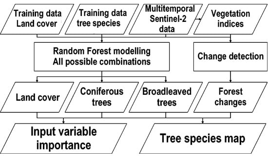
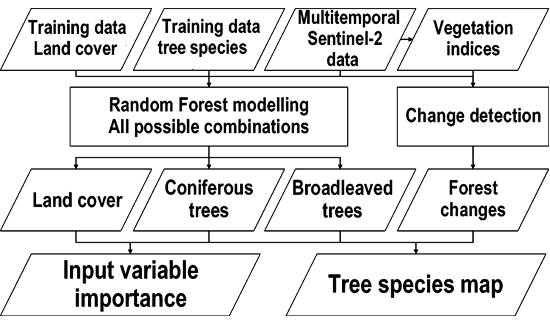
For the land cover classification and the tree species mapping in the Wienerwald biosphere reserve, 18 cloud-free Sentinel-2 scenes acquired between 2015 and 2017 were used. The mapping was done in three steps using different reference data sets (Figure 1). In the first step, six broad land cover classes were mapped. Subsequently, the individual tree species were identified within the resulting forest strata. In the final step, change detection was applied to identify areas where forest activities took place.

For the broad land cover classification, reference data were visually interpreted in a regular grid using four-band orthoimages with a spatial resolution of 20 cm acquired in the course of the national aerial image campaign and provided by Austria’s Federal Office of Metrology and Surveying. The reference data for the tree species were derived from stand maps and other forest management databases. To enhance the data quality, the reference points were cross-checked by visual interpretation of color-infrared (CIR) orthoimages. With these reference data, the coniferous and broadleaved tree species were classified both separately and together, while testing all possible combinations of the Sentinel-2 data. The best classification results were merged together and areas where changes could be detected were masked out.

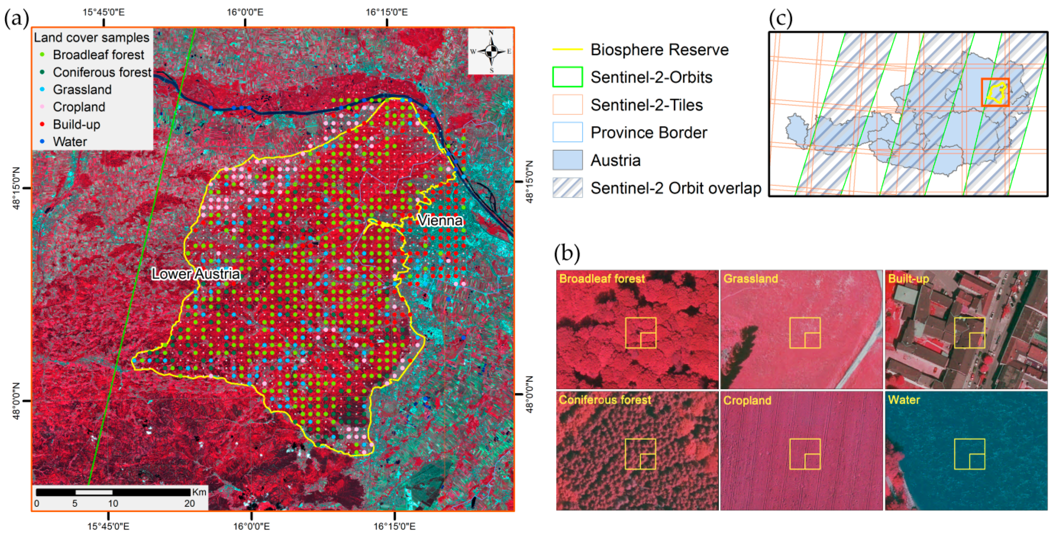
2.1. Study Site Wienerwald Biosphere Reserve

The Wienerwald biosphere reserve is one of the largest contiguous deciduous beech woodlands in Central Europe. It is located in the south-west of Vienna (Austria) and covers an area of 105,645 ha. The location of such a large forest on the edge of a metropolitan area is unique. The range of (micro) climatic and geological conditions in the Wienerwald is the main reason for the large diversity of vegetation types [35]. The Biosphere Reserve has more than 20 types of woodland—with beech, oak and hornbeam being dominant—and more than 23 types of meadow [36]. Concerning the forest, particularly rare woods can be found, such as Austrian’s largest downy oak forests (Quercus pubescens) and unique stands of Austrian Black Pine (Pinus nigra subsp. nigra) occurring in the eastern part of the Wienerwald [37]. The inlet in Figure 2 shows the location of the study area within a region characterized by its diversity of nature and culture, and sustainable ecosystem management.

2.2. Reference Data Sets

For the reference data creation, a regular grid (1 km × 1 km) was laid over the entire biosphere reserve as well as some surrounding areas (Figure 2a). At each point, the grid cell was visually interpreted using CIR orthoimages (Figure 2b).

Table 1. Summary of the reference data for the land cover classification.

Class Name	Definition	Samples	Amount [%]
Broadleaf forest	Broadleaf-dominated forests	388	48.68
Coniferous forest	Conifer-dominated forests	97	12.17
Grassland	Grassland, meadows, lawns, pastures, parks, etc.	104	13.05
Cropland	Agricultural crops, wine yards	77	9.66
Built-up	Sealed surfaces - buildings, roads, infrastructure, etc.	116	14.56
Water	Lakes, rivers, ponds, etc.	15	1.88
	$\sum$	797	100.00

presents the number of samples and class definitions of the six land cover classes.

Six target classes were distinguished for the land cover classification: deciduous forest, broadleaf forest, grassland, cropland, build-up areas and water bodies. To receive adequate numbers of trainings samples for the classes cropland, build-up areas and water, the grid was extended to surrounding areas in the north and east of the study area. Only clearly interpretable samples which contain only one class were retained for the training of the classification model. In the end, 797 out of 1360 pixels were useable.

For the tree species classification, additional reference samples were necessary and were derived from forest management data. First, pure stands of the 12 tree species were identified in the forest management maps. Next, one or two Sentinel-2 pixels were chosen in the center of each stand and the correctness of the information was checked using CIR orthoimages (Figure 3).

In this way, on average 85 reference samples per tree species were distinguished, well distributed over the entire biosphere reserve (

Table 2. Summary of the reference data for the tree species classification.

Tree Species	Scientific Name	Acronym	Samples	Amount [%]
European beech	Fagus sylvatica	FS	215	21.37
European alder	Alnus glutinosa	AG	52	5.17
European ash	Fraxinus excelsior	FE	60	5.96
Oaks	Quercus sp.	QU	130	12.92
Cherry	Prunus sp.	PR	25	2.49
European hornbeam	Carpinus betulus	CP	65	6.46
Maple	Acer sp.	AC	33	3.28
Norway spruce	Picea abies	PA	135	13.42
Austrian pine	Pinus nigra	PN	107	10.64
Scots pine	Pinus sylvestris	PS	79	7.85
European larch	Larix decidua	LD	49	4.87
Douglas fir	Pseudotsuga menziesii	PM	56	5.57
		∑	1006	100.00

). The variation in the number of available reference data reflects the difficulties to identify sufficiently large and pure stands for some of the species.

2.3. Sentinel-2 Data Sets

The study area is located in the overlapping area of two Sentinel-2 orbits (122 and 79—Figure 2), and therefore, the number of acquisitions twice as high as normal in this latitude. For the analysis, all available Sentinel-2 scenes were visually checked. Only cloud-free data were selected. From the 188 scenes acquired between June 2015 to end of 2017, 18 scenes were perfectly useable. Summary information about selected scenes can be found in

Table 3. Summary of the selected Sentinel-2 data sets (granule T33UWP). Over the region of interest, the images were free of clouds. The percentage cloud cover of the entire scenes was in the range 0-15%.

Sentinel-2 Satellite	Date	Orbit	Sun Zenith Angle	Sun Azimuth Angle
A	30.08.2015	122	40.64	160.67
A	25.12.2015	79	72.89	165.72
A	27.03.2016	122	46.92	161.03
A	13.04.2016	79	40.99	157.03
A	06.05.2016	122	32.93	159.34
A	31.08.2016	79	41.81	157.47
A	13.09.2016	122	45.77	164.04
A	30.09.2016	79	52.43	164.31
A	11.01.2017	122	71.18	165.83
A	01.04.2017	122	45.04	160.96
A	28.05.2017	79	29.06	151.92
A	20.06.2017	122	26.83	153.18
A	01.08.2017	79	33.19	150.41
A	29.08.2017	122	40.48	160.55
A	08.09.2017	122	43.90	162.88
A	28.09.2017	122	51.20	167.02
B	30.09.2017	79	52.35	164.20
A	15.10.2017	79	57.79	166.70

. All scenes were atmospherically corrected using Sen2Cor [38] Version 2.4 using the data service platform operated by BOKU [39] on the Earth Observation Data Centre (EODC) [40]. The 20 m bands B5, B6, B7, B8a, B11 and B12 were resampled to 10 m and the 60 m-bands B1, B9 and B10 were excluded from the analyses.

2.4. Random Forest Classification Approach

For all classifications, the ensemble learning random forest (RF) approach developed by Breiman [41] was used. The two hyper-parameters mtry (number of predictors randomly sampled for each node) and ntree (the number of trees) were set to the square root of available input variables (default) and, to 1000, respectively.

One advantage of the bootstrapping is that it yields relatively unbiased ‘out-of-bag’ (OOB) results, as long as representative reference data are provided [42]. Another benefit is the computation of importance measures which can be used for the evaluation of the input data and subsequent feature reduction. In this study, a recursive feature selection process using the ‘Mean decrease in Accuracy’ (MDA) was applied similarly to other studies [18,43,44]. More information about the algorithm and its advantages, such as the importance measure for the input variables and the integrated bootstrapping, can be found in the literature [16,41,45,46].

To classify the six land cover classes, first a model based on all Sentinel-2 datasets was developed using the land cover reference data from the visually interpreted regular grid. The tree species models were developed separately for the broadleaf and coniferous species—for testing purposes we also pooled all tree species together. The tree species classification models were based on the tree species reference data set and only applied to areas previously mapped as broadleaf or coniferous forest.

To find the best combinations for the tree species classification, we tested all possible combinations of the 18 Sentinel-2 scenes. We tested for example 18 individual scenes, 153 combinations of two scenes, 816 of three and so on. In total, 262,143 different models for each of the two forest strata were developed. The training of each model, including the feature selection, took on average about 5 min on a standard PC (CPU i7-2600 3.40 GHz, 16 GB RAM), and therefore, a high-performance computing (HPC) environment was used.

The modeling was done with two data sets: one contains only the 10 spectral bands, the second combines the 10 spectral bands with 28 widely used vegetation indices (

Table A1. Overview of the used vegetation indices and band combinations together with the corresponding formula and references (band 8 was used for the NIR = Near − Infrared; RE = Red − Edge).

Name	Formula	Reference
Built-up Area Index (BAI)	$\frac{\mathit{BLUE}-\mathit{NIR}}{\mathit{BLUE}+\mathit{NIR}}$	[61]
Chlorophyll Green index (CGI)	$\frac{\mathit{NIR}}{\mathit{GREEN}+\mathit{RE}1}$	[62]
Global Environmental Monitoring Index (GEMI)	$\eta -0.25{\eta }^2-\frac{\mathit{RED}-0.125}{1-\mathit{RED}}$ $\eta =\frac{2\left(NI{R}^2-RE{D}^2\right)+1.5NIR+0.5RED}{NIR+RED+0.5}$	[63]
Greenness Index (GI)	$\frac{\mathit{GREEN}}{\mathit{RED}}$	[64]
Green Normalized Difference Vegetation Index (gNDVI)	$\frac{\mathit{NIR}-\mathit{GREEN}}{\mathit{NIR}+\mathit{GREEN}}$	[65]
Leaf Chlorophyll Content Index (LCCI)	$\frac{\mathit{RE}3}{\mathit{RE}1}$	[29]
Moisture Stress Index (MSI)	$\frac{\mathit{SWIR}1}{\mathit{NIR}}$	[66]
Normalized Difference Red-Edge and SWIR2 (NDRESWIR)	$\frac{\mathit{RE}2-\mathit{SWIR}2}{\mathit{RE}2+\mathit{SWIR}2}$	[67]
Normalized Difference Tillage Index (NDTI)	$\frac{\mathit{SWIR}1-\mathit{SWIR}2}{\mathit{SWIR}1+\mathit{SWIR}2}$	[68]
Normalized Difference Vegetation Index (NDVI)	$\frac{\mathit{NIR}-\mathit{RED}}{\mathit{NIR}+\mathit{RED}}$	[69]
Red-Edge Normalized Difference Vegetation Index (reNDVI)	$\frac{\mathit{NIR}-\mathit{RE}1}{\mathit{NIR}+\mathit{RE}1}$	[65]
Normalized Difference Water Index 1 (NDWI1)	$\frac{\mathit{NIR}-\mathit{SWIR}1}{\mathit{NIR}+\mathit{SWIR}1}$	[70]
Normalized Difference Water Index 2 (NDWI2)	$\frac{\mathit{NIR}-\mathit{SWIR}2}{\mathit{NIR}+\mathit{SWIR}2}$	[65]
Normalized Humidity Index (NHI)	$\frac{\mathit{SWIR}1-\mathit{GREEN}}{\mathit{SWIR}1+\mathit{GREEN}}$	[71]
Red-Edge Peak Area (REPA)	$\mathit{RED}+\mathit{RE}1+\mathit{RE}2+\mathit{RE}3+\mathit{NIR}$	[67,72]
Red SWIR1 Difference (DIRESWIR)	$\mathit{RED}-\mathit{SWIR}1$	[73]
Red-Edge Triangular Vegetation Index (RETVI)	$100(\mathit{NIR}-\mathit{RE}1)-10(\mathit{NIR}-\mathit{GREEN})$	[74]
Soil Adjusted Vegetation Index (SAVI)	$\frac{\mathit{NIR}-\mathit{RED}}{\mathit{NIR}+\mathit{RED}+0.5}1.5$	[75]
Blue and RE1 ratio (SRBRE1)	$\frac{\mathit{BLUE}}{\mathit{RE}1}$	[64]
Blue and RE2 ratio (SRBRE2)	$\frac{\mathit{BLUE}}{\mathit{RE}2}$	[76]
Blue and RE3 ratio (SRBRE3)	$\frac{\mathit{BLUE}}{\mathit{RE}3}$	[67]
NIR and Blue ratio (SRNIRB)	$\frac{\mathit{NIR}}{\mathit{BLUE}}$	[77]
NIR and Green ratio (SRNIRG)	$\frac{\mathit{NIR}}{\mathit{GREEN}}$	[64]
NIR and Red ratio (SRNIRR)	$\frac{\mathit{NIR}}{\mathit{RED}}$	[77]
NIR and RE1 ratio (SRNIRRE1)	$\frac{\mathit{NIR}}{\mathit{RE}1}$	[62]
NIR and RE2 ratio (SRNIRRE2)	$\frac{\mathit{NIR}}{\mathit{RE}2}$	[67]
NIR and RE3 ratio (SRNIRR3)	$\frac{\mathit{NIR}}{\mathit{RE}3}$	[67]
Soil Tillage Index (STI)	$\frac{\mathit{SWIR}1}{\mathit{SWIR}2}$	[68]
Water Body Index (WBI)	$\frac{\mathit{BLUE}-\mathit{RED}}{\mathit{BLUE}+\mathit{RED}}$	[78]

in the Appendix A).

2.5. Input Data Evaluation

The classification models were assessed using the OOB results. Previous studies had demonstrated that the OOB results of RF classifiers compare well against an assessment based on a separate validation data set [42,47,48].

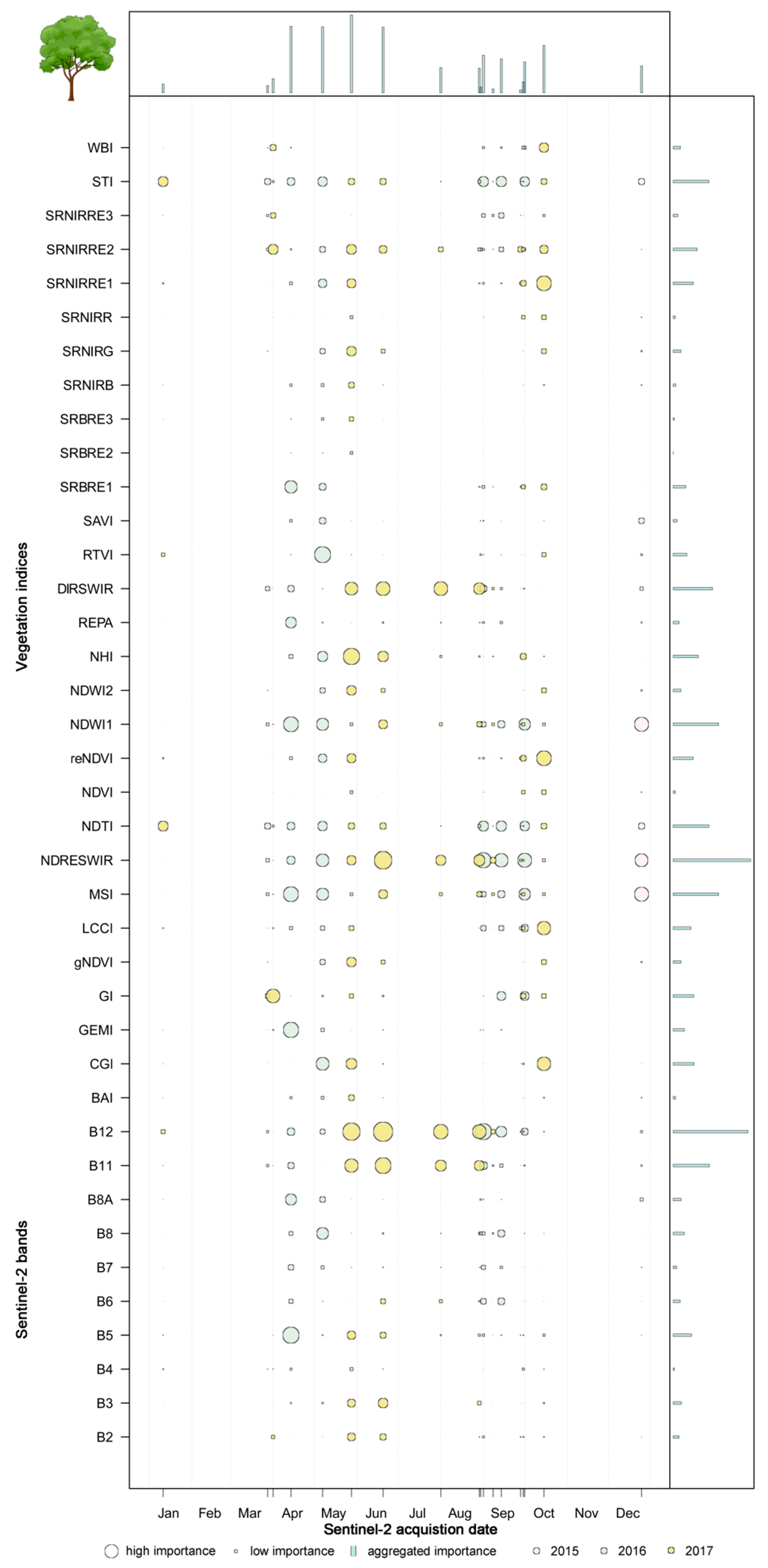
To assess the importance of individual Sentinel-2 bands and acquisition times, the ‘Mean decrease in Accuracy’ (MDA) importance values of the final RF models (after feature selection) were normalized for each model to 1 by dividing all values by the maximum value of the specific model. Variables which were eliminated by the feature selection procedure were assigned an importance value of 0. All normalized values were summed up for all tested combinations and divided by the total number of tested combinations (Equation (1)):

$${\mathit{IMP}}_i=\frac{{{\displaystyle \sum }}_{j=0}^n\frac{{\mathit{MDA}}_{\mathit{ji}}}{{\mathit{MDA}}_{\mathit{jmax}}}}{n}$$

(1)

where IMP_i is the normalized and aggregated importance value for variable i (= one band of one specific Sentinel-2 scene); MDA_ji the MDA importance value of variable i in the model j; MDA_jmax the maximum MDA importance value in the model j; and n the number of models (combinations of Sentinel-2 scenes) considering variable i (= 131,072).

When evaluating the importance of the spectral bands, models involving the vegetation indices were discarded to avoid skewing the results by the chosen indices. This was deemed particularly important as most indices include the NIR band. However, we applied the evaluation also to the models with vegetation indices to investigate the most important vegetation indices for tree species classification.

2.6. Change Detection

As outlined above, for the tree species classification, data from a three-year period (2015 to 2017) were used. To avoid interference of possibly occurring changes during the three years, a simple change detection was applied. Changes in the forest cover were detected by comparing the NDVI values from the respective August scenes of the years 2015, 2016 and 2017. Based on the difference between the NDVI of the actual and the previous year, pixels with absolute differences of ≤0.05 were flagged as ‘change’. Negative values indicate a decrease in leaf biomass and were interpreted as an indicator of forest management activities such as thinning, harvesting or calamities. This interpretation was cross-checked by visual interpretation of the data sets and consultations with the forest management. All areas where forest management activities were detected were masked out from the tree species map.

3. Results

3.1. Land Cover Classification

The land cover classification based on all input data using the random forest modeling approach including the feature selection achieved an overall accuracy of 96%, and nearly all class-specific accuracies were higher than 90% (

Table 4. Confusion matrix based on OOB results of the land cover classification model based on all 18 Sentinel-2 scenes. (UA: user’s accuracy, PA: producer’s accuracy, OA: overall accuracy).

		Reference
		BF	CF	GL	CL	BU	WB	UA
Classification	Broadleaf forest (BF)	387	7	2	0	2	0	97.3%
	Conifer forest (CF)	0	90	0	0	0	0	100.0%
	Grassland (GL)	1	0	94	5	0	0	94.0%
	Cropland (CL)	0	0	6	70	3	0	88.6%
	Build-up (BU)	0	0	2	2	111	0	96.5%
	Waterbody (WB)	0	0	0	0	0	15	100.0%
	∑ reference data	388	97	104	77	116	15	797
	PA	99.7%	92.8%	90.4%	90.9%	95.7%	100%
			OA		96.2%	Kappa	0.946

). The highest misclassifications can be found between the two agricultural classes grassland and cropland. The two forest classes (broadleaf and conifer forest) achieved very high producer and user accuracies (>93%).

3.2. Tree Species Classification

The boxplots in Figure 4 illustrate the overall accuracies based on the out-of-bag results after feature selection. Each bar summarizes the different image combinations (1–18 images). For the coniferous species (middle row), overall accuracies of around 90% were achieved. Occasionally, a combination of five to six scenes was sufficient for such high classification accuracies. For the broadleaf trees (top row), the overall accuracies leveled out at around 80%. Here, a slightly higher number of scenes was necessary to reach optimum performance (7–8 scenes). The OA of the model trained on the pooled set of tree species was somewhere between the two class-specific results (bottom row). In all three cases, the use of vegetation indices (right column) improved the classification compared to the sole use of the reflectance data (left column). The average improvement of the OA was around 5 percentage points: The highest OA of the best models improved from 82.1% to 85.9% for the broadleaf strata, from 90.4% to 95.3% for the coniferous strata and from 83.5% to 88.7% for all tree species pooled together. Compared to the best mono-temporal results the use of multi-temporal data (both including vegetation indices) improved the out-of-bag overall accuracy from 72.9% to 85.7% for the broadleaved, from 83.8% to 95.3% for the coniferous and from 74.4% to 88.7% for all tree species together.

The best results for the broadleaf trees obtained an overall accuracy of 86%. For all species, the achieved Producer’s and User’s accuracies are good (>70%) to very good (>90%) except for maple (Acer sp.). For the coniferous the best model reached an overall accuracy of 95.3%. All class specific accuracies were above 90%. For comparison reason the two results of the best broadleaf and the best coniferous models were combined into a single confusion matrix in

Table 5. Confusion matrix based on the combined OOB results of the best broadleaf and the best coniferous model using spectral bands and vegetation indices. (UA: user’s accuracy, PA: producer’s accuracy, OA: overall accuracy).

		Reference
		FS	AG	FE	QU	PR	CP	AC	PA	PN	PS	LD	PM	UA
Classification	Fagus sylvatica (FS)	211	4	7	7	4	12	8						83.4%
	Alnus glutinosa (AG)	0	44	0	1	0	0	0						97.8%
	Fraxinus excelsior (FE)	0	0	44	3	0	0	7						81.5%
	Quercus sp. (QU)	0	1	5	117	1	4	2						90.0%
	Prunus sp. (PR)	0	0	0	0	18	0	0						100.0%
	Carpinus betulus (CB)	4	2	3	1	1	48	0						81.4%
	Acer sp. (AC)	0	1	1	1	1	1	16						76.2%
	Picea abies (PA)								132	0	3	1	1	96.4%
	Pinus nigra (PN)								1	101	1	1	2	95.3%
	Pinus sylvestris (PS)								1	4	75	0	0	93.8%
	Larix decidua (LD)								1	1	0	46	1	93.9%
	Pseudotsuga menziesii (PM)								0	1	0	1	52	96.3%
	∑ Reference data	215	52	60	130	25	65	33	135	107	79	49	56
	PA	98.1%	84.6%	73.3%	90.0%	72.0%	73.8%	48.5%	97.8%	94.4%	94.9%	93.9%	92.9%
								OA	89.9%		Kappa	0.885

. The differences to the result of the best model including all tree species (

Table 6. Confusion matrix based on the OOB result of the best model for all tree species together using spectral bands and vegetation indices. (UA: user’s accuracy, PA: producer’s accuracy, OA: overall accuracy).

		Reference
		FS	AG	FE	QU	PR	CP	AC	PA	PN	PS	LD	PM	UA
Classification	Fagus sylvatica (FS)	210	3	4	7	4	11	8	0	0	0	0	0	85.0%
	Alnus glutinosa (AG)	0	43	0	1	0	0	1	0	0	0	0	0	95.6%
	Fraxinus excelsior (FE)	0	0	46	2	0	0	7	0	0	0	0	0	83.6%
	Quercus sp. (QU)	2	2	7	115	1	4	2	1	0	0	0	0	85.8%
	Prunus sp. (PR)	0	0	1	0	17	0	0	0	0	0	1	0	89.5%
	Carpinus betulus (CB)	2	3	0	3	2	49	0	0	0	0	0	0	83.1%
	Acer sp. (AC)	0	1	2	1	1	1	15	0	0	0	0	0	71.4%
	Picea abies (PA)	0	0	0	0	0	0	0	132	0	3	1	5	93.6%
	Pinus nigra (PN)	0	0	0	0	0	0	0	1	98	1	1	1	96.1%
	Pinus sylvestris (PS)	0	0	0	0	0	0	0	1	7	74	1	0	89.2%
	Larix decidua (LD)	1	0	0	1	0	0	0	0	2	1	45	2	86.5%
	Pseudotsuga menziesii (PM)	0	0	0	0	0	0	0	0	0	0	0	48	100.0%
	∑ Reference data	215	52	60	130	25	65	33	135	107	79	49	56
	PA	97.7%	82.7%	76.7%	88.5%	68.0%	75.4%	45.5%	97.8%	91.6%	93.7%	91.8%	85.7%
								OA	88.7%		Kappa	0.871

) are small. The aggregated overall accuracy of the stratified approach is slightly higher (89.9% versus 88.7%) and some classes with small numbers of reference data also benefit from the separated modeling. The best models for the three groups are based on the following input data after feature selection: (1) broadleaf trees: 159 variables from nine dates including all spectral bands and indices, (2) coniferous trees: 24 variables from seven dates including three bands and 13 indices, (3) all tree species together: 126 variables from 13 dates including eight bands and 26 indices.

Huge differences in feature importance were found within and between the model tree species groups (Figure 5). The dot size indicates the importance of a specific band (y-axis) and date (x-axis) in the classification models. Larger dots indicate a higher importance. To generate this information, the results of all combinations were aggregated, excluding models with vegetation indices. For the broadleaf species, the most important Sentinel-2 bands are the SWIR bands B12 and B11 followed by the Red-Edge band 1 (B5) and acquisitions from May, April and June are more useful compared to those from late summer and autumn. For the coniferous species, a higher number of scenes showed high importance compared to the broadleaf species. Again, the acquisition End of May, as well as the August acquisitions, showed the highest contribution. For the separation of the coniferous species the Red band is the most relevant band. The results for the aggregated modeling with all tree species together is a mixture of the results of the modeling for the two strata. Only the high importance of the NIR band B8 is striking.

Similar results can be found for the models using spectral data and vegetation indices together. For all three groups, the same Sentinel-2 bands show the highest importance (Figure A1, Figure A2 and Figure A3). The vegetation indices with the highest contributions to the classification performance for the broadleaf species were again indices which consider the SWIR, NIR and Red-Edge bands in different variations such as simple ratios, differences, and normalized differences (Figure A1). For the coniferous species mainly indices based on the NIR and Red bands (simple ratios and normalized differences) and the ratio between Green and Red showed the highest importance values (Figure A2). The result for all tree species together is again a mixture of the two strata. The highest ranked variable in the aggregated modeling was the Difference between Red and SWIR (Figure A3).

Figure 6 shows the final result of the tree species mapping for the entire Wienerwald biosphere reserve. The map combines the results of the land cover classification, the stratified tree species models (separated for broadleaf and coniferous species) and the change detection (forest management activities).

A qualitative check was done by the biosphere reserve management and the validity was confirmed. The different forest types mainly result from geological differences (e.g., Black pine forests in the southeast grow on limestone) and different management strategies (e.g., higher amount of coniferous trees in other regions).

For the detection of forest changes, the simple comparison of NDVI values from August scenes of different years was useful, as for each year, changes were captured on around 1% of the forest area. Areas where changes were detected in first period (2015–2016) often showed a clear regrowth in the second period. First trials aggregating the values to stand maps and interpreting the absolute values showed promising results to distinguish between different forest management activities (not shown). Both the affected area and the grade of the thinning can be determined based on the change in the NDVI values and the number of pixels with changes.

4. Discussion

4.1. Classification Accuracy

The classification of 12 tree species revealed very good results. We obtained an overall accuracy of 89% in line with comparable studies. However, most of the previous studies used only three to five S2 scenes and considered only fewer classes: Nelson [32] achieved 86% for six tree species classes, Bolyn et al. [22] 92% for 11 forest classes, Wessel et al. [33] 88% for four tree species classes, Persson et al. [27] 88% for five tree species, Soleimannejad et al. [49] 77% for three tree species and Hościło and Lewandowska [34] 76% (using only S2 bands) and 85% (using a stratified approach and including topographic features), for eight tree species. Grabska et al. [23] achieved with five (out of 18) S2 scenes an overall accuracy of 92% for nine tree species. We attribute our favorable results to the high quality of the reference data and the acquisition density, which allowed covering the temporal changes in the spectral signatures well, which in turn contributed to the successful classifications.

Several studies showed that higher accuracies can be achieved using data with higher spatial resolution such as WorldView-2 or Pleiades [25,26,49]. The accuracies of the present study are even higher compared to studies using WorldView-2 data for tree species classification under similar ecological conditions. For example, Immitzer et al. [16] obtained for 10 tree species overall accuracies of 82%, Waser et al. [17] for seven species 83% and Fassnacht et al. [15] for 10 species 80%. In the present study, we found clear indications that the use of multi-temporal data contributed to the successful classifications, further enhanced by the availability of spectral bands in the SWIR.

Only maple, cherry and European hornbeam were classified with low accuracies (46–75%). All other classes reached high (≥77%) to very high (≥85%) producer’s and user’s accuracies. Coniferous species were generally very well identified, in line with results published by Grabska et al. [23] and in contrast to Hościło and Lewandowska [34]. Further research is warranted to determine why not all species show distinct spectral-temporal features.

Similar to other studies [15,16,23,24,25,30], we found that class imbalances negatively affect the class-specific results. For ‘hard-to-separate classes’, the class with more samples is obviously preferred by the RF classifier and consequently obtains higher accuracies. This underlines again the importance of an adequate number of high quality reference samples. Although desirable, in practice, such a request is not always feasible, as some tree species hardly occur in pure stands, respectively, do not cover large enough areas for being detectable with 10 m resolution data.

4.2. Acquisition Date

In particular for the multi-date classifications, it is difficult to depict the importance of the acquisition date, as counter-balancing effects occur. For example, for mono-temporal classifications, the dataset from May achieved the best result for all tree species together. Images acquired in May were also used in models achieving the highest accuracies based on combinations of two and more scenes, together with October images. The sole use of October images, however, gave only moderate results. Hence, whereas individual acquisition dates can be well interpreted in mono-temporal classification, this is not always possible when multiple scenes are involved. To sustain interpretation, we aggregated the feature importance information in a new way (Equation (1) and Figure 5). As a general trend we confirm findings of previous studies, that a well-balanced data set, involving scenes from spring to autumn, are preferable [23,34,50]. When enough processing power and storage is available, a simple straight forward solution is to use all available images. Obviously, for very large areas such an approach will fail, as clouds will occur at least in parts of the area, making it necessary to use either compositing techniques [51] or spatio-temporal gap-filling procedures [52].

Species-specific temporal changes of the spectral signatures can be visualized nicely using dense time-series [23]. The date of leaf flush, for example, varies from species to species. This permits to distinguish tree species that otherwise show very similar spectral signatures during the summer months. The same holds for the timing of the leaf coloration. Therefore, both phenomena can be very helpful for the separation of tree species [23,50,53,54,55,56,57]. However, regional differences related to altitude, aspect or soil conditions co-influence the phenological development and timing of leaf flush and coloration, making additional information necessary [58]. Therefore, the quality of the available reference data is very important, as well as means to define strata in which individual models perform well. Alternatively, one has to use (auxiliary) proxy variables describing the species-independent phenological variations that are typically encountered when working across larger regions [59].

In general terms, it is beneficial to acquire and use large representative samples for each species covering as good as possible the site-specific variations. To leverage species-dependent differences in phenological development, the highest possible revisit frequencies are optimum. Very dense time series not only mitigate cloud effects but also permit to extract key phenological indicators such as start and end of season [50,60]. In our study, the available cloud-free scenes did not cover the entire year in regular intervals: mainly in July, only very few cloud-free data sets were acquired due to convective cloud formation; additionally, in spring and autumn, spells of bad weather prevented the acquisition of useful scenes.

4.3. Sentinel-2 Bands and Vegetation Indices

Our study demonstrates the high suitability of the Sentinel-2 bands for the separation of broad land cover classes as well as for the identification of various tree species. The most important bands are the SWIR, Red and NIR. The importance of the NIR and SWIR bands for species classification was also highlighted by other studies [22,27,28,49]. Our results reveal that the SWIR bands are mainly necessary for the separation of the individual broadleaf species; the NIR band is useful for the separation of the two strata coniferous and broadleaf species. In our work, the broader NIR band (band 8 at 10 m) achieves higher importance values than the narrow NIR band (band 8a at 20 m). This is in contrast to the work of Bolyn et al. [22] and Persson et al. [27], who found that band 8a was more important. Additionally, these two studies and Grabska et al. [23] highlighted the significance of the Red-Edge bands, which cannot be fully confirmed by our study. As the mentioned bands are recorded at different spatial resolutions, the contradictions may stem from site-specific differences in the patchiness of the forests. On the other hand, the high importance of the Red band for the coniferous species is in agreement with Hościło and Lewandowska [34].

We found that the use of vegetation indices improved the classification performance compared to the sole use of spectral signatures. Similar results were reported by Puletti et al. [28] and Maschler et al. [12]. The most relevant vegetation indices were based on the same bands, which show high importance in the models based only on spectral bands. For the broadleaf species, band combinations involving the SWIR, NIR and Red Edge bands were most useful, for the coniferous indices based on Red and NIR bands. The highest ranked indices considering all types of indices (simple ratios, differences, normalize differences).

5. Conclusions

The introduced Sentinel-2 workflow for tree species classification is robust, cost-efficient and scalable. The workflow was already successfully applied in several test areas across Germany. In the highly diverse Wienerwald biosphere reserve in Austria, the classification method achieved high classification accuracies for most of the 12 investigated tree species. However, a noticeable dependence on tree species, but also on the number and quality of the reference data, was found.

The NIR band is useful to separate the two tree species groups, coniferous and broadleaf trees, but much less so for identifying individual species. For the identification of the seven broadleaf species, the two SWIR bands are the most important. To separate the five individual coniferous species, the highest importance was found for the Red band. The use of additional vegetation indices further improved the performance of the classification models, and is therefore highly recommended.

The sensors on-board of Sentinel-2A and 2B provide rich spectral information in 10 spectral bands. The data are extremely useful for tree species mapping over large areas. The data is freely available, and due to the regular and dense acquisition pattern (five-day), images covering all phenological stages can be acquired and used for the classification. Although a few well-placed acquisitions can possibly yield very good classification results, the easiest way to ensure high classification accuracies is to combine and use all available cloud-free images simultaneously. This avoids the definition of the ‘perfect’ acquisition date(s), which far too often cannot be obtained due to local weather conditions.

With two Sentinel-2 satellites and their high revisit rate, the acquisition of several scenes per year should be possible for most Central European regions. However, especially over mountainous regions such as the Alps, the revisit frequency is probably still not high enough. The high cloudiness also prevents the application of methods for the extraction of land surface phenology (LSP) parameters, and their subsequent use in classification models. Unfortunately, in mountainous regions such as the Alps, microwave sensors are also only of limited use, due to strong terrain effects and radar shadows. Hence, it is requested to further increase the temporal revisit frequency of optical sensors and to make better use of virtual constellations, if possible involving the fleet of commercial VHR satellites.

From a methodological point of view, research should focus on further increasing the number of tree species involved in such classifications, while finding ways to handle strong class imbalances and missing values. The handling of mixed classes should also have high priority, as long as sensor resolution does not permit to resolve individual tree crowns. Ultimately, the full benefits of Earth Observation data will only become visible if such maps are produced and regularly updated at continental scale. This requires progress in terms of data standardization and feature extraction, and implementation of suitable code within HPC environments having direct access to the data storage. More research is warranted to identify the bio-physical factors leading to the observed large variations in species-specific classification accuracies.

References

1. IPBES. Summary for policymakers of the global assessment report on biodiversity and ecosystem services of the Intergovernmental Science-Policy Platform on Biodiversity and Ecosystem Services; Díaz, S., Settele, J., Brondizio, E.S., Ngo, H.T., Guèze, M., Agard, J., Arneth, A., Balvanera, P., Brauman, K.A., Butchart, S.H.M., et al., Eds.; IPBES secretariat: Bonn, Germany, 2019; p. 45. [Google Scholar]
2. Kuenzer, C.; Ottinger, M.; Wegmann, M.; Guo, H.; Wang, C.; Zhang, J.; Dech, S.; Wikelski, M. Earth observation satellite sensors for biodiversity monitoring: Potentials and bottlenecks. Int. J. Remote Sens. 2014, 35, 6599–6647. [Google Scholar] [CrossRef]
3. Nagendra, H. Using remote sensing to assess biodiversity. Int. J. Remote Sens. 2001, 22, 2377–2400. [Google Scholar] [CrossRef]
4. Pettorelli, N.; Wegmann, M.; Skidmore, A.; Mücher, S.; Dawson, T.P.; Fernandez, M.; Lucas, R.; Schaepman, M.E.; Wang, T.; O’Connor, B.; et al. Framing the concept of satellite remote sensing essential biodiversity variables: Challenges and future directions. Remote Sens. Ecol. Conserv. 2016, 2, 122–131. [Google Scholar] [CrossRef]
5. Pettorelli, N.; Safi, K.; Turner, W. Satellite remote sensing, biodiversity research and conservation of the future. Phil. Trans. R. Soc. B 2014, 369, 20130190. [Google Scholar] [CrossRef] [PubMed]
6. Kissling, W.D.; Walls, R.; Bowser, A.; Jones, M.O.; Kattge, J.; Agosti, D.; Amengual, J.; Basset, A.; van Bodegom, P.M.; Cornelissen, J.H.C.; et al. Towards global data products of Essential Biodiversity Variables on species traits. Nat. Ecol. Evol. 2018, 2, 1531–1540. [Google Scholar] [CrossRef] [PubMed] [Green Version]
7. Schlerf, M.; Atzberger, C. Inversion of a forest reflectance model to estimate structural canopy variables from hyperspectral remote sensing data. Remote Sens. Environ. 2006, 100, 281–294. [Google Scholar] [CrossRef]
8. Lindenmayer, D.B.; Margules, C.R.; Botkin, D.B. Indicators of biodiversity for ecologically sustainable forest management. Conserv. Biol. 2000, 14, 941–950. [Google Scholar] [CrossRef]
9. Wulder, M.A.; Hall, R.J.; Coops, N.C.; Franklin, S.E. High spatial resolution remotely sensed data for ecosystem characterization. BioScience 2004, 54, 511–521. [Google Scholar] [CrossRef]
10. Dalponte, M.; Ørka, H.O.; Ene, L.T.; Gobakken, T.; Næsset, E. Tree crown delineation and tree species classification in boreal forests using hyperspectral and ALS data. Remote Sens. Environ. 2014, 140, 306–317. [Google Scholar] [CrossRef]
11. Fassnacht, F.; Neumann, C.; Forster, M.; Buddenbaum, H.; Ghosh, A.; Clasen, A.; Joshi, P.; Koch, B. Comparison of Feature Reduction Algorithms for Classifying Tree Species With Hyperspectral Data on Three Central European Test Sites. IEEE J. Sel. Top. Appl. Earth Obs. Remote Sens. 2014, 7, 2547–2561. [Google Scholar] [CrossRef]
12. Maschler, J.; Atzberger, C.; Immitzer, M. Individual Tree Crown Segmentation and Classification of 13 Tree Species Using Airborne Hyperspectral Data. Remote Sens. 2018, 10, 1218. [Google Scholar] [CrossRef]
13. Peerbhay, K.Y.; Mutanga, O.; Ismail, R. Commercial tree species discrimination using airborne AISA Eagle hyperspectral imagery and partial least squares discriminant analysis (PLS-DA) in KwaZulu–Natal, South Africa. ISPRS J. Photogramm. Remote Sens. 2013, 79, 19–28. [Google Scholar] [CrossRef]
14. Carleer, A.; Wolff, E. Exploitation of very high resolution satellite data for tree species identification. Photogramm. Eng. Remote Sens. 2004, 70, 135–140. [Google Scholar] [CrossRef]
15. Fassnacht, F.E.; Mangold, D.; Schäfer, J.; Immitzer, M.; Kattenborn, T.; Koch, B.; Latifi, H. Estimating stand density, biomass and tree species from very high resolution stereo-imagery—Towards an all-in-one sensor for forestry applications? For. Int. J. For. Res. 2017, 90, 613–631. [Google Scholar] [CrossRef]
16. Immitzer, M.; Atzberger, C.; Koukal, T. Tree species classification with Random Forest using very high spatial resolution 8-band WorldView-2 satellite data. Remote Sens. 2012, 4, 2661–2693. [Google Scholar] [CrossRef]
17. Waser, L.T.; Küchler, M.; Jütte, K.; Stampfer, T. Evaluating the Potential of WorldView-2 Data to Classify Tree Species and Different Levels of Ash Mortality. Remote Sens. 2014, 6, 4515–4545. [Google Scholar] [CrossRef] [Green Version]
18. Immitzer, M.; Böck, S.; Einzmann, K.; Vuolo, F.; Pinnel, N.; Wallner, A.; Atzberger, C. Fractional cover mapping of spruce and pine at 1ha resolution combining very high and medium spatial resolution satellite imagery. Remote Sens. Environ. 2018, 204, 690–703. [Google Scholar] [CrossRef]
19. Metzler, J.W.; Sader, S.A. Model development and comparison to predict softwood and hardwood per cent cover using high and medium spatial resolution imagery. Int. J. Remote Sens. 2005, 26, 3749–3761. [Google Scholar] [CrossRef]
20. EEA Forests—Copernicus Land Monitoring Service. Available online: http://land.copernicus.eu/pan-european/high-resolution-layers/forests (accessed on 8 February 2017).
21. Fassnacht, F.E.; Latifi, H.; Stereńczak, K.; Modzelewska, A.; Lefsky, M.; Waser, L.T.; Straub, C.; Ghosh, A. Review of studies on tree species classification from remotely sensed data. Remote Sens. Environ. 2016, 186, 64–87. [Google Scholar] [CrossRef]
22. Bolyn, C.; Michez, A.; Gaucher, P.; Lejeune, P.; Bonnet, S. Forest mapping and species composition using supervised per pixel classification of Sentinel-2 imagery. Biotechnol. Agron. Soc. Environ. 2018, 22, 172–187. [Google Scholar]
23. Grabska, E.; Hostert, P.; Pflugmacher, D.; Ostapowicz, K. Forest Stand Species Mapping Using the Sentinel-2 Time Series. Remote Sens. 2019, 11, 1197. [Google Scholar] [CrossRef]
24. Immitzer, M.; Vuolo, F.; Atzberger, C. First Experience with Sentinel-2 Data for Crop and Tree Species Classifications in Central Europe. Remote Sens. 2016, 8, 166. [Google Scholar] [CrossRef]
25. Immitzer, M.; Vuolo, F.; Einzmann, K.; Ng, W.-T.; Böck, S.; Atzberger, C. Verwendung von multispektralen Sentinel-2 Daten für die Baumartenklassifikation und Vergleich mit anderen Satellitensensoren. In Proceedings of the Beiträge zur 36. Wissenschaftlich-Technischen Jahrestagung der DGPF, Bern, Switzerland, 7–9 June 2016; Volume 25. [Google Scholar]
26. Ng, W.-T.; Rima, P.; Einzmann, K.; Immitzer, M.; Atzberger, C.; Eckert, S. Assessing the Potential of Sentinel-2 and Pléiades Data for the Detection of Prosopis and Vachellia spp. in Kenya. Remote Sens. 2017, 9, 74. [Google Scholar] [CrossRef]
27. Persson, M.; Lindberg, E.; Reese, H. Tree Species Classification with Multi-Temporal Sentinel-2 Data. Remote Sens. 2018, 10, 1794. [Google Scholar] [CrossRef]
28. Puletti, N.; Chianucci, F.; Castaldi, C. Use of Sentinel-2 for forest classification in Mediterranean environments. Ann. Silvic. Res. 2018, 42, 32–38. [Google Scholar]
29. Wulf, H.; Stuhler, S. Sentinel-2: Land Cover, Preliminary User Feedback on Sentinel-2A Data. In Proceedings of the Sentinel-2A Expert Users Technical Meeting, Frascati, Italy, 29–30 September 2015; pp. 29–30. [Google Scholar]
30. Sheeren, D.; Fauvel, M.; Josipović, V.; Lopes, M.; Planque, C.; Willm, J.; Dejoux, J.-F. Tree Species Classification in Temperate Forests Using Formosat-2 Satellite Image Time Series. Remote Sens. 2016, 8, 734. [Google Scholar] [CrossRef]
31. Gómez, C.; White, J.C.; Wulder, M.A. Optical remotely sensed time series data for land cover classification: A review. ISPRS J. Photogramm. Remote Sens. 2016, 116, 55–72. [Google Scholar] [CrossRef] [Green Version]
32. Nelson, M. Evaluating Multitemporal Sentinel-2 Data for Forest Mapping Using Random Forest. Master’s Thesis, Stockholm University, Stockholm, Sweden, 2017. [Google Scholar]
33. Wessel, M.; Brandmeier, M.; Tiede, D. Evaluation of Different Machine Learning Algorithms for Scalable Classification of Tree Types and Tree Species Based on Sentinel-2 Data. Remote Sens. 2018, 10, 1419. [Google Scholar] [CrossRef]
34. Hościło, A.; Lewandowska, A. Mapping Forest Type and Tree Species on a Regional Scale Using Multi-Temporal Sentinel-2 Data. Remote Sens. 2019, 11, 929. [Google Scholar] [CrossRef]
35. Staudinger, M.; Scheiblhofer, J. Artenreichtum, Artenverteilung und räumliche Aspekte der Biodiversität der Gefäßpflanzen in Wäldern des Biosphärenpark Wienerwald. Wiss. Mitteilungen Niederösterreichischen Landesmus. 2014, 25, 249–268. [Google Scholar]
36. Mrkvicka, A.; Drozdowski, I.; Brenner, H. Kernzonen im Biosphärenpark Wienerwald—Urwälder von morgen. Wiss. Mitteilungen Niederösterreichischen Landesmus. 2014, 25, 41–88. [Google Scholar]
37. Drozdowski, I.; Mrkvicka, A. Der Wienerwald ist UNESCO-Biosphärenpark—Eine Modellregion für Nachhaltigkeit. Wiss. Mitteilungen Niederösterreichischen Landesmus. 2014, 25, 9–40. [Google Scholar]
38. Pflug, B.; Bieniarz, J.; Debaecker, V.; Louis, J.; Müller-Wilms, U. Some experience using sen2cor. In Proceedings of the EGU General Assembly Conference Abstracts, Vienna, Austria, 17–22 April 2016; Volume 18. [Google Scholar]
39. Vuolo, F.; Żółtak, M.; Pipitone, C.; Zappa, L.; Wenng, H.; Immitzer, M.; Weiss, M.; Baret, F.; Atzberger, C. Data Service Platform for Sentinel-2 Surface Reflectance and Value-Added Products: System Use and Examples. Remote Sens. 2016, 8, 938. [Google Scholar] [CrossRef]
40. Bucur, A.; Wagner, W.; Elefante, S.; Naeimi, V.; Briese, C. Development of an Earth Observation Cloud Platform in Support to Water Resources Monitoring. In Earth Observation Open Science and Innovation; Mathieu, P.-P., Aubrecht, C., Eds.; ISSI Scientific Report, Series; Springer International Publishing: Cham, Switzerland, 2018; pp. 275–283. ISBN 978-3-319-65633-5. [Google Scholar] [Green Version]
41. Breiman, L. Random forests. Mach. Learn. 2001, 45, 5–32. [Google Scholar] [CrossRef]
42. Toscani, P.; Immitzer, M.; Atzberger, C. Texturanalyse mittels diskreter Wavelet Transformation für die objektbasierte Klassifikation von Orthophotos. Photogramm. Fernerkund. Geoinf. 2013, 2, 105–121. [Google Scholar] [CrossRef]
43. Guyon, I.; Weston, J.; Barnhill, S.; Vapnik, V. Gene Selection for Cancer Classification using Support Vector Machines. Mach. Learn. 2002, 46, 389–422. [Google Scholar] [CrossRef]
44. Einzmann, K.; Immitzer, M.; Böck, S.; Bauer, O.; Schmitt, A.; Atzberger, C. Windthrow Detection in European Forests with Very High-Resolution Optical Data. Forests 2017, 8, 21. [Google Scholar] [CrossRef]
45. Hastie, T.; Tibshirani, R.; Friedman, J. The Elements of Statistical Learning: Data Mining, Inference, and Prediction, 2nd ed.; Springer: New York, NY, USA, 2009; ISBN 978-0-387-84858-7. [Google Scholar]
46. Pal, M. Random forest classifier for remote sensing classification. Int. J. Remote Sens. 2005, 26, 217–222. [Google Scholar] [CrossRef]
47. Vuolo, F.; Neuwirth, M.; Immitzer, M.; Atzberger, C.; Ng, W.-T. How much does multi-temporal Sentinel-2 data improve crop type classification? Int. J. Appl. Earth Obs. Geoinf. 2018, 72, 122–130. [Google Scholar] [CrossRef]
48. Belgiu, M.; Drăguţ, L. Random forest in remote sensing: A review of applications and future directions. ISPRS J. Photogramm. Remote Sens. 2016, 114, 24–31. [Google Scholar] [CrossRef]
49. Soleimannejad, L.; Ullah, S.; Abedi, R.; Dees, M.; Koch, B. Evaluating the potential of sentinel-2, landsat-8, and irs satellite images in tree species classification of hyrcanian forest of iran using random forest. J. Sustain. For. 2019, 38, 615–628. [Google Scholar] [CrossRef]
50. Pasquarella, V.J.; Holden, C.E.; Woodcock, C.E. Improved mapping of forest type using spectral-temporal Landsat features. Remote Sens. Environ. 2018, 210, 193–207. [Google Scholar] [CrossRef]
51. Pflugmacher, D.; Rabe, A.; Peters, M.; Hostert, P. Mapping pan-European land cover using Landsat spectral-temporal metrics and the European LUCAS survey. Remote Sens. Environ. 2019, 221, 583–595. [Google Scholar] [CrossRef]
52. Vuolo, F.; Ng, W.-T.; Atzberger, C. Smoothing and gap-filling of high resolution multi-spectral time series: Example of Landsat data. Int. J. Appl. Earth Obs. Geoinf. 2017, 57, 202–213. [Google Scholar] [CrossRef]
53. Elatawneh, A.; Rappl, A.; Rehush, N.; Schneider, T.; Knoke, T. Forest tree species identification using phenological stages and RapidEye data: A case study in the forest of Freising. In Proceedings of the 5th RESA Workshop, From the Basics to the Service, DLR e.V., Neustrelitz, Germany, 20–21 March 2013; pp. 21–38. [Google Scholar]
54. Hill, R.A.; Wilson, A.K.; George, M.; Hinsley, S.A. Mapping tree species in temperate deciduous woodland using time-series multi-spectral data. Appl. Veg. Sci. 2010, 13, 86–99. [Google Scholar] [CrossRef]
55. Lisein, J.; Pierrot-Deseilligny, M.; Bonnet, S.; Lejeune, P. A Photogrammetric Workflow for the Creation of a Forest Canopy Height Model from Small Unmanned Aerial System Imagery. Forests 2013, 4, 922–944. [Google Scholar] [CrossRef] [Green Version]
56. Schriever, J.R.; Congalton, R.G. Evaluating seasonal variability as an aid to cover-type mapping from Landsat Thematic Mapper data in the Northeast. Photogramm. Eng. Remote Sens. 1995, 61, 321–327. [Google Scholar]
57. Stoffels, J.; Hill, J.; Sachtleber, T.; Mader, S.; Buddenbaum, H.; Stern, O.; Langshausen, J.; Dietz, J.; Ontrup, G. Satellite-Based Derivation of High-Resolution Forest Information Layers for Operational Forest Management. Forests 2015, 6, 1982–2013. [Google Scholar] [CrossRef]
58. Li, D.; Ke, Y.; Gong, H.; Li, X. Object-Based Urban Tree Species Classification Using Bi-Temporal WorldView-2 and WorldView-3 Images. Remote Sens. 2015, 7, 16917–16937. [Google Scholar] [CrossRef] [Green Version]
59. Mascaro, J.; Asner, G.P.; Knapp, D.E.; Kennedy-Bowdoin, T.; Martin, R.E.; Anderson, C.; Higgins, M.; Chadwick, K.D. A Tale of Two “Forests”: Random Forest Machine Learning Aids Tropical Forest Carbon Mapping. PLoS ONE 2014, 9, e85993. [Google Scholar] [CrossRef]
60. Guerif, M.; Gu, X.F.; Inra, J.P.G. Crop-system characterization by multitemporal SPOT data in the South-East of France. Int. J. Remote Sens. 1992, 13, 1843–1851. [Google Scholar] [CrossRef]
61. Shahi, K.; Shafri, H.Z.M.; Taherzadeh, E.; Mansor, S.; Muniandy, R. A novel spectral index to automatically extract road networks from WorldView-2 satellite imagery. Egypt. J. Remote Sens. Space Sci. 2015, 18, 27–33. [Google Scholar] [CrossRef] [Green Version]
62. Datt, B. A New Reflectance Index for Remote Sensing of Chlorophyll Content in Higher Plants: Tests using Eucalyptus Leaves. J. Plant Physiol. 1999, 154, 30–36. [Google Scholar] [CrossRef]
63. Pinty, B.; Verstraete, M.M. GEMI: A non-linear index to monitor global vegetation from satellites. Vegetatio 1992, 101, 15–20. [Google Scholar] [CrossRef]
64. Le Maire, G.; François, C.; Dufrêne, E. Towards universal broad leaf chlorophyll indices using PROSPECT simulated database and hyperspectral reflectance measurements. Remote Sens. Environ. 2004, 89, 1–28. [Google Scholar] [CrossRef]
65. Gitelson, A.A.; Kaufman, Y.J.; Merzlyak, M.N. Use of a green channel in remote sensing of global vegetation from EOS-MODIS. Remote Sens. Environ. 1996, 58, 289–298. [Google Scholar] [CrossRef]
66. Vogelmann, J.E.; Rock, B.N. Spectral Characterization of Suspected Acid Deposition Damage in Red Spruce (picea Rubens) Stands from Vermont. In Proceedings of the Airborne Imaging Spectrometer Data Anal. Workshop, Pasadena, CA, USA, 8–10 April 1985; pp. 51–55. [Google Scholar]
67. Radoux, J.; Chomé, G.; Jacques, D.C.; Waldner, F.; Bellemans, N.; Matton, N.; Lamarche, C.; d’Andrimont, R.; Defourny, P. Sentinel-2′s Potential for Sub-Pixel Landscape Feature Detection. Remote Sens. 2016, 8, 488. [Google Scholar] [CrossRef]
68. Van Deventer, A.P.; Ward, A.D.; Gowda, P.M.; Lyon, J.G. Using thematic mapper data to identify contrasting soil plains and tillage practices. Photogramm. Eng. Remote Sens. 1997, 63, 87–93. [Google Scholar]
69. Tucker, C.J. Red and photographic infrared linear combinations for monitoring vegetation. Remote Sens. Environ. 1979, 8, 127–150. [Google Scholar] [CrossRef] [Green Version]
70. Gao, B. NDWI—A normalized difference water index for remote sensing of vegetation liquid water from space. Remote Sens. Environ. 1996, 58, 257–266. [Google Scholar] [CrossRef]
71. Lacaux, J.P.; Tourre, Y.M.; Vignolles, C.; Ndione, J.A.; Lafaye, M. Classification of ponds from high-spatial resolution remote sensing: Application to Rift Valley Fever epidemics in Senegal. Remote Sens. Environ. 2007, 106, 66–74. [Google Scholar] [CrossRef]
72. Filella, I.; Penuelas, J. The red edge position and shape as indicators of plant chlorophyll content, biomass and hydric status. Int. J. Remote Sens. 1994, 15, 1459–1470. [Google Scholar] [CrossRef]
73. Jacques, D.C.; Kergoat, L.; Hiernaux, P.; Mougin, E.; Defourny, P. Monitoring dry vegetation masses in semi-arid areas with MODIS SWIR bands. Remote Sens. Environ. 2014, 153, 40–49. [Google Scholar] [CrossRef]
74. Chen, P.-F.; Tremblay, N.; Wang, J.-H.; Vigneault, P.; Huang, W.-J.; Li, B.-G. New index for crop canopy fresh biomass estimation. Spectrosc. Spectr. Anal. 2010, 30, 512–517. [Google Scholar]
75. Huete, A.R. A soil-adjusted vegetation index (SAVI). Remote Sens. Environ. 1988, 25, 295–309. [Google Scholar] [CrossRef]
76. Lichtenthaler, H.; Lang, M.; Sowinska, M.; Heisel, F.; Miehé, J. Detection of Vegetation Stress Via a New High Resolution Fluorescence Imaging System. J. Plant Physiol. 1996, 148, 599–612. [Google Scholar] [CrossRef]
77. Blackburn, G.A. Quantifying Chlorophylls and Caroteniods at Leaf and Canopy Scales: An Evaluation of Some Hyperspectral Approaches. Remote Sens. Environ. 1998, 66, 273–285. [Google Scholar] [CrossRef]
78. Domenech, E.; Mallet, C. Change Detection in High resolution land use/land cover geodatabases (at object level). EuroSDR Off. Publ. 2014, 64. [Google Scholar]
Figure 1. Workflow diagram of the classification approach with three main steps: (1) broad land cover classification, (2) tree species identification within the forest strata and (3) change detection to mask out areas where forest activities took place.
Remotesensing 11 02599 g001
Figure 2. Overview of the study area and the 6-class land cover reference data. (a) Regular grid for reference data collection for the land cover classification covering the biosphere reserve and some surrounding areas (background: Sentinel-2 bands 8-4-3). (b) Examples (10 and 20 m grid cells) for each class (background: CIR orthoimage). (c) Location of the biosphere reserve Wienerwald within Austria and Sentinel-2 orbit cover.
Remotesensing 11 02599 g002
Figure 3. (a) Distribution of the reference data set for the tree species classification and (b) examples (10 and 20 m grid cells) for each tree species. Background images: Color Infrared composites of Sentinel-2 (a) and orthoimages (b).
Remotesensing 11 02599 g003
Figure 4. Overall accuracies of all possible Sentinel-2 combinations based on models using only spectral bands (ac) and using spectral bands and vegetation indices (df). Strata-specific results are displayed in the rows: results for broadleaf species (a,d), coniferous species (b,e) and all tree species together (c,f).
Remotesensing 11 02599 g004
Figure 5. Aggregated feature importance derived from the combination of all classification models, excluding models involving spectral vegetation indices. A larger dot size indicates a higher importance of the specific band and date combination. The bars on the top and right side of the graphs summarize the importance of the individual months and spectral bands, respectively. (a) Results for the broadleaf stratum, (b) coniferous species and (c) all tree species pooled together. Different colors indicate the year of the Sentinel-2 acquisition.
Remotesensing 11 02599 g005
Figure 6. Final map based on aggregation of the best models of the land cover, broadleaf trees and coniferous trees classifications and the results of the change detection.
Remotesensing 11 02599 g006