Study on Sea Clutter Suppression Methods Based on a Realistic Radar Dataset

Department of Space Physics, School of Electronic Information, Wuhan University, Wuhan 430072, China
*
Author to whom correspondence should be addressed.
Remote Sens. 2019, 11(23), 2721; https://doi.org/10.3390/rs11232721
Submission received: 15 October 2019
/
Revised: 7 November 2019
/
Accepted: 18 November 2019
/
Published: 20 November 2019
Abstract
:To improve the ability of radar to detect targets such as ships with a background of strong sea clutter, different sea-clutter suppression algorithms are developed based on the realistic Intelligent PIxel processing X-band (IPIX) radar datasets, and quantitative research is carried out. Four algorithms, namely root cycle cancellation, singular-value decomposition (SVD) suppression, wavelet weighted reconstruction, and empirical mode decomposition (EMD) weighted reconstruction and their corresponding suppression methods are introduced. Then, the differences between the four algorithms before and after sea-clutter suppression are compared and analyzed. The average clutter-suppression and target-suppression amplitudes are selected as measures to verify the suppression effect. Sea-clutter data collected in the high-sea state, low-sea state, near-sea area, and far-sea area are selected for statistical analysis after suppression. All four methods have certain suppression effects, among which EMD reconstruction is best, reaching an average clutter-suppression range of 15.507 dB and a signal-suppression range of about 1 dB, which can improve the ability of radar to detect targets such as ships with a background of strong sea clutter.

1. Introduction
The rough undulating sea surface interacts with the electromagnetic waves emitted by radar to produce backscattered echoes with strong energy [1,2,3]. These echoes are called sea clutter. After a matching filter and Doppler processing, the Range-Doppler (RD) spectrum of sea clutter mainly shows that the ridge lines with frequency symmetry (the two strongest of these ridges lines in the spectrum are called the first-order Bragg peak), and not necessarily the same amplitude, are scattered in each distance unit [4], which often leads to a serious drop in the radar’s ability to detect targets [5]. Especially for the sky-wave radar, due to the limitation of Doppler resolution, the first-order scattering spectrum of sea clutter in the Doppler domain appears as a clutter signal near zero frequency, which seriously affects the detection of ship targets. The clutter is in the target environment, and its signal is intertwined with the target signal entering the receiver. It is difficult to improve the signal-to-noise ratio (SNR) through system design. Moreover, the causes of sea clutter are complicated [3]. The sea surface is mainly composed of two types of waves: tension waves and gravity waves. Sea surface environmental factors, including wind speed, sea current, swell, temperature, and humidity, will affect its shape. Echo sea clutter can vary, with different choices for the parameters in the radar system. Sea clutter can also vary widely. Therefore, changes in the sea clutter signal are complicated, echo intensity is high, and clutter is difficult to handle. When the target’s radar cross-section (RCS) is less than or equal to the RCS of the sea surface in the radar detection range, strong sea clutter will interfere with the radar’s detection of the target [6,7], thereby increasing the difficulty of sea clutter suppression [8,9].
Methods of suppressing sea clutter can be divided into two major categories. A typical method of the first type is the time-domain cancellation method, represented by the root loop cancellation method [10,11]. The core idea of this method is to utilize the frequency or power spectrum of the signal to be detected to estimate the relevant parameters (amplitude, frequency, and initial phase) of the sea clutter’s sinusoidal signal, thereby reconstructing the sea clutter in the time domain and subtracting it from the echo signal to achieve clutter suppression. The second is based on the subspace projection class method [12,13], which is typically represented by singular-value decomposition (SVD) [14]. The main idea of this method is to obtain the clutter subspace and then to suppress sea clutter through subspace projection.
Wavelet transform is a time–frequency analysis method for multi-resolution analysis [15,16]. This method can realize high-resolution local positioning in both the time and frequency domains and is good at extracting transient and steady-state information, as well as signal waveform characteristics in non-stationary signals. Huang et al. proposed the empirical mode decomposition (EMD) algorithm [17], a multiresolution analysis method based on local features of the time domain, which has proven to be a good non-stationary, nonlinear signal method. It is widely used for the analysis of mechanical vibrations, waves, structural mechanics, and natural seismic signals [16,17,18,19,20,21]. Since the signal frequency processed by the algorithm is transient and belongs to the category of local waves, it is also called a local wave decomposition algorithm. This algorithm’s advantage is that it is completely data-driven, and the base functions come from the data itself.
In this paper, four commonly used sea clutter suppression algorithms are quantitatively analyzed and compared. In Section 2, the principles and basic processing flows of the four algorithms are simplified. Section 3 shows the comparison and analysis of four different methods for the Intelligent PIxel processing X-band (IPIX) radar dataset. In Section 4, the results of different sea clutter suppression algorithms are statistically analyzed for different sea areas, sea conditions, and rubbing angles. We summarize the article in Section 5.
2. Sea Clutter Suppression Algorithms
2.1. Root Cycle Cancellation Algorithm Principle
The cyclic cancellation method is a short dwell time sea clutter suppression algorithm proposed by Root in 1998 [10]. When the radar phase difference accumulation time is short, a first-order Bragg peak can be simulated with two harmonic components. The cyclic cancellation algorithm uses a fast Fourier transform to estimate the amplitude, frequency, and initial phase of the two harmonic components [11], reconstructs the two components in the time domain, and subtracts the received echo signals. These two harmonic components are used for sea clutter suppression. The difficulty of this algorithm is in correctly estimating the parameters of the harmonic components. This estimation, reconstruction, and subtraction must be repeated several times to complete the suppression of sea clutter to make the signal stand out. The root cycle cancellation algorithm is as follows.
The time-domain signal of the radar echo in a certain distance gate is , and the echo signal is fast Fourier transformed to obtain . We then obtain the maximum point of falling in the frequency range of the clutter. The amplitude , corresponding to the extreme point, and the angular frequency are estimated as parameters of the first component signal, as follows:
Using the principle of minimum residual energy, the initial phase is searched in the range of to determine the phase of the clutter component that minimizes
The first clutter component extracted by the above calculation can be expressed as:
The component is then removed from the original radar echo time-domain signal to obtain the residual signal:
The above process is repeated for the remaining signals until the target signal can be found.
2.2. Principle of the Singular-Value Decomposition (SVD) Algorithm
Because sea clutter can be seen as a narrow-band time-varying signal, a Hankel matrix can be constructed with the time-domain signal of the radar echo, and SVD can be performed on it. The singular value generated by decomposition can be traced to the frequency component corresponding to the first-order Bragg peak, and the suppression of the sea clutter is completed by setting the singular value of the corresponding sea clutter to zero [14]. Since the SVD algorithm performs multiple matrix decomposition and reconstruction calculations, its speed is relatively slow. When the algorithm is applied, the selection of the suppression range of sea clutter can also be difficult. If the selected suppression range is small, the sea clutter will not be completely suppressed. On the contrary, if the selected range is too large, the target signal may not be detected, resulting in radar leakage. The SVD algorithm is as follows.
Suppose the radar echo signal of a certain distance gate is , where , and is the data length of . The form of the Hankel matrix is:
where is the number of columns of the Hankel matrix. In general, , where is the number of sinusoidal signals contained in the sequence . After constructing the Hankel matrix, the algorithm proceeds as follows:
- Perform SVD on the matrix , i.e., .
- For each nonzero singular value on the diagonal of the singular value matrix , reconstruct the time series corresponding to the singular value. The reconstruction process is as follows. For the singular value matrix , only can be reserved, and other singular values are set to zero. is recovered by . The back-diagonal elements of the matrix are used for averaging to reconstruct the time series, i.e., , where , and is the number of elements in the back-diagonal of the matrix, i.e., the number of elements that conform to .
- A Fourier transform is performed for the time-domain sequence . If the spectral peak of the frequency-domain sequence obtained after the Fourier transform falls within the first-order Bragg frequency band, we can consider the singular value to correspond to the frequency component of the first-order Bragg peak. Then, the singular value is set to zero to complete the suppression of sea clutter. In this way, we obtain a new singular value matrix .
- The reconstructed time series is recovered by using the singular value matrix, , which is the time-domain signal sequence after clutter suppression.
2.3. Principles of Wavelet Algorithm
A one-dimensional discrete wavelet transform is a basic analysis method based on MRA (multi-resolution analysis), which can be used as an effective tool to separate one-dimensional signals of different scales (widening degrees) [15,16]. Jangal proposed a method to decompose the RD (Range-Doppler) spectrum of HF (high frequency) ground wave radar into the wavelet domain and to perform ionospheric clutter suppression by weighted reconstruction using wavelet analysis [15]. In 2009, to refine and improve the wavelet method, a complex radar signal was further processed by one- and two-dimensional wavelet transform to suppress ionospheric clutter. This method not only obtained a better clutter suppression effect but improved the SNR by about 20 dB. The author also discussed how to use wavelet analysis to extract sea clutter in the RD spectrum to obtain useful oceanographic parameters [22]. However, the signal-processing performance for drowning in the clutter is weak. When the signal-to-clutter ratio of a target signal is less than 5 dB, it cannot be extracted from the clutter. Moreover, processing, such as the selection of a wavelet and the decomposition layer of the wavelet function, relies on empirical parameters and cannot be fully realized in some specific engineering applications. The wavelet reconstruction algorithm is as follows.
Let the basic wavelet be , and its Fourier transform . If satisfies the tolerance condition , then the discrete wavelet basis function is:
where is the scale factor, and is the translation coefficient.
The one-dimensional discrete wavelet transform coefficients for any function can be expressed as:
where, is a locally oscillating base on which the signal is projected, and the frequency distribution of the local time is obtained. is a stretched transformation with , i.e., when the scale is smaller, the corresponding frequency is higher, and the time resolution is higher, but the frequency resolution is lower. Therefore, the one-dimensional discrete wavelet transform can perform a multi-resolution analysis on the local features of signals and is suitable for radar Doppler spectrum analysis with different scales of signals and local singular features.
Select “db3” as the criterion of the wavelet base and the wavelet transform processing object as the data after distance processing, beamforming, and Doppler processing. The frequency-domain signal of each range gate is then processed. Set the Doppler spectrum of the currently processing -th range gate as .
- Wavelet decomposition: Wavelet transform is performed on to obtain the wavelet coefficient . Let the number of wavelet decomposition layers be , and .
- Wavelet single-branch reconstruction: The wavelet coefficient of each layer is reconstructed by a single branch. The single reconstructed signal of the layer is:where is the wavelet reconstruction coefficient.
- Let each layer of the single reconstructed signals form a single reconstructed function vector :
- Weighted merging: Let the wavelet domain of the pure target be , and normalize the weighting coefficient as:Let the weighting coefficient vector be . Then, the weighted combined Doppler spectrum is:
The Doppler spectrum of each distance gate is combined into an RD spectrum, which is the RD spectrum after clutter suppression.
2.4. Principles of the Empirical Mode Decomposition (EMD) Reconstruction Algorithm
Wavelet transform depends on the base function, whose selection directly affects the ability of these methods to analyze the signal. A signal that is compatible with the selected basis function gives a better analysis result. However, in reality, the signal itself is ever-changing, and it is impossible to find a base signal that can be adapted to all signals. In this context, Huang et al. of NASA (National Aeronautics and Space Administration) proposed the EMD algorithm in 1998 [18]. The base functions required for data analysis are adaptively obtained from specific data by the EMD algorithm. The result of EMD decomposition forms an approximately orthogonal intrinsic mode function (IMF). The IMF is the signal that satisfies the following two conditions:
- In the whole data set, the number of extrema and the number of zero crossings must either be equal or differ at most by one.
- At any point, the mean value of the envelope defined by the local maxima and the envelope defined by the local minima is zero.
The first condition is similar to the traditional narrow band requirements for a stationary Gaussian process. The second condition is a new constraint proposed by Huang et al., which changes the traditional global condition to a local condition to avoid unnecessary fluctuations in the instantaneous frequency due to the asymmetry of the signal waveform. In an ideal case, the condition should be “the local mean of the data being zero.” However, for non-stationary data, the “local mean” involves a “local time scale”, and a definition is impossible. Therefore, they use the local mean of the envelopes defined by the local maxima and the local minima to force local symmetry instead. This definition does not necessarily guarantee that the results are completely correct, but Huang et al. verified that the instantaneous frequency obtained by this method is physically significant even under worst-case conditions. The IMF under this definition makes it easier to calculate the correct instantaneous frequency.
The method of decomposing a composite signal into its IMF components is called EMD. This decomposition is based on three assumptions:
- The signal has at least two extrema—one maximum and one minimum.
- The characteristic time scale is defined by the time lapse between the extrema. If the data are totally devoid of extrema but contain only inflection points, then they can be differentiated once or more to reveal the extrema. The final results can be obtained by integrating the components.
The specific steps of the EMD algorithm are:
- For any real signal or data , firstly, find all the local maxima and local minima points of . Then, interpolate all maxima and all minima. Afterwards, we can obtain the upper envelope and the lower envelope of the signal and calculate their average curves :
- Subtract from to get :
- If does not satisfy the conditions of the IMF, define the average envelope of as . Subtract from to get :This process may be repeated k times:where and are the signals obtained by the -th and ()th screenings, respectively, and is the average envelope of . When the IMF conditions are met, .
- Subtract from , and we obtain a new signal , from which the high-frequency component is removed:
- Substitute for and repeat the above steps. Then, we obtain in sequence. This screening is stopped when satisfies the given termination condition. is called the residual, which represents the trend of the signal. Finally, can be expressed as the sum of a set of IMF components and a residual [23,24]:The criteria for terminating the screening, is expressed as:
In practical applications, a reasonable range for is 0.2–0.3, which not only ensures the stability of EMD decomposition but prevents excessive decomposition. In this paper, . For complex signals, complex EMD methods are needed for decomposition [25,26]. Complex EMD is divided into positive- and negative-frequency elements. Before performing this division, we construct a new signal by using the positive- and negative-frequency elements of the Doppler spectrum and convert the two realized signals via an inverse Fourier transform.
The EMD processing and wavelet transform processing steps are basically the same, but the EMD-processed signal is the time-domain signal, and since the frequency of each mode component decreases as the decomposition order increases, the high-frequency component is not the main sea clutter. We are mainly concerned with the sea clutter component near the low and zero frequencies, so the high-frequency components are not weighted and are directly merged.
3. Sea Clutter Suppression based on Intelligent PIxel Processing X-Band (IPIX) Radar Data
3.1. Experimental Data
The sea clutter data used in this paper are the IPIX radar sea clutter data from McMaster University in Canada. The main parameters of the IPIX radar are shown in Table 1 [27]. The IPIX radar has two public sea clutter databases, consisting of data collected by Dartmouth in 1993 and Grimsby in 1998. Most of the data in 1993 used 131.072 s for each distance gate (i.e., 131,072 data points) and 14 distance gates for a single experiment. In 1998, the data sampling time was 60.00 s (i.e., 60,000 data points). We used totally 28 range gates in each single experiment.
We selected the fifth range gate data for the 287th data-acquisition experiment of the 1993 experimental database. The ocean has a significant wave height of 0.8 m (maximum 1.3 m), and the sea state is 2 (according to the sea state rating defined by the World Meteorological Organization). Thus, the results of this experiment can be regarded as low-sea-state sea clutter data. The polarization mode of this experiment is VV polarization, which means the transmitting terminal is a vertically polarized antenna, and the receiving terminal is also a vertically polarized antenna. The horizontal distance between the sampling range gate and the antenna is 1320 m, so the radar beam wiping angle can be calculated to be about 1.302°. A fractional Fourier transform (FFT) is performed on the data. Using a hamming window, the width of the window is 4096 data points (about four seconds), the window moving distance is 1024 data points (about 1 s), and the FFT point is 512 points. The time–frequency (or time-Doppler) image of a single range gate and the sea clutter spectrum at 10 s can be obtained, as shown in Figure 1 and Figure 2.
It can be seen that the sea clutter exhibits a strong clutter component near the zero frequency and an elevation of the base noise around the zero frequency in the spectrum.
3.2. Sea Clutter Suppression under Different Sea Conditions
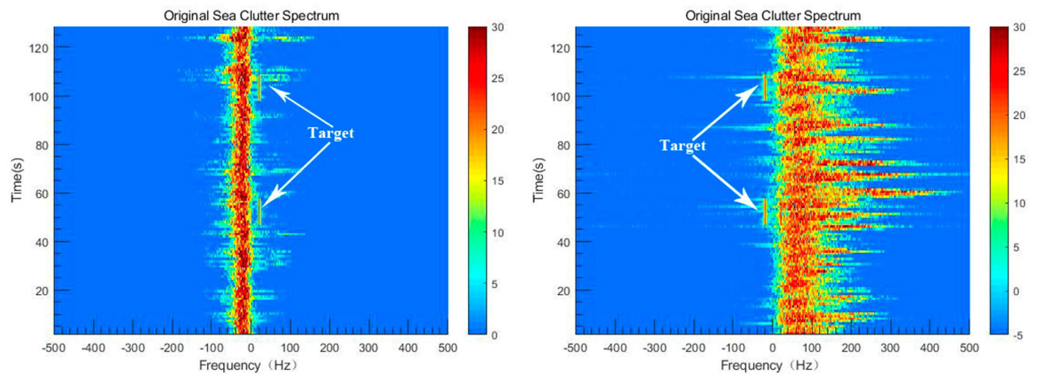
For clutter suppression under different sea conditions, we used the data of the fifth range gate of the 287th data-acquisition experiment from the 1993 database for the low-sea-state data, and the third range gate data of the 269th data acquisition for the high-sea-state data. The low-sea-state data have been introduced before and will not be repeated. The ocean in high-sea-state data acquisition has 1.8 m (maximum 2.9 m) of significant wave height, the sea state is 4, and the horizontal distance between the range gate and the antenna is 930 m, so the radar beam wipes the ground. The angle can be calculated to be approximately 1.845°. Adding the virtual target at 45–55 s and 95–105 s of the data, the frequency is ±20 Hz. The virtual target added this time is the single-frequency signal, one of which is “hidden” by the clutter component (one can also add a chirp signal as a virtual target). Time–frequency images in the high and low sea conditions are shown in Figure 3.
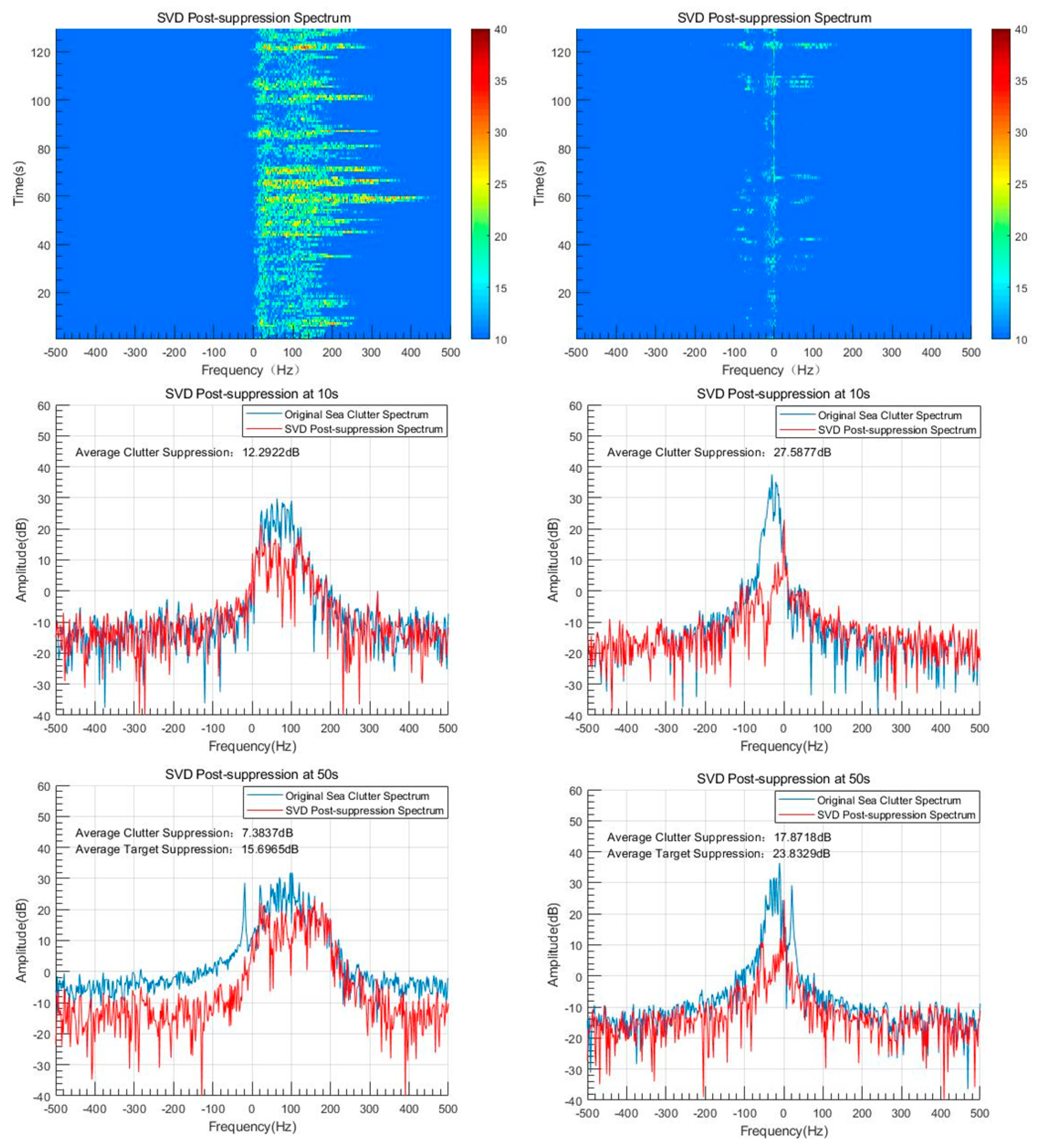
It can be seen that in high sea conditions, the low-frequency sea clutter component near the zero frequency broadens more, the clutter component is stronger, the target signal is more likely to be hidden in the clutter spectrum, and the target is less likely to be detected by the radar. We will suppress these two groups of data using the four methods mentioned above and observe the inhibitory effect. We determined the time–frequency image after suppression of the signal of each window and extracted a spectrogram before and after the suppression at different times. The extracted time is 50 s (with virtual target) and 10 s (without virtual target and for comparison). We calculated the spectrum comparison map before and after suppression, the average suppression amplitude of the main components of the clutter, and the suppression range of the target frequency, as shown in Figure 4, Figure 5, Figure 6 and Figure 7.
Root cycle cancellation occurs 60 times. In the low-sea-state, the loop cancellation method suppresses a part of the low-frequency sea-clutter strong component, and a certain suppression effect is obtained. However, in high sea conditions, since the sea-clutter component has a wide spread in the spectrum, the root cycle cancels only a small part of the low-frequency sea-clutter strong component. The first-order Bragg peak is used to simulate the root cycle cancellation method with two harmonic components, and it is impossible to distinguish whether the two harmonic peaks on the spectrum are the target or the first-order Bragg peak. Thus, the target frequency is easily eliminated, and sometimes the SNR is not improved.
C is the number of columns of the Hankel matrix constructed by singular-value decomposition (SVD), and its value is , where r is the number of sinusoidal signals contained in the sampled signal, and N is the length of the sampled data (here, it is the length of the window). If C is too small, then the Hankel matrix will be close to the singular value or the scaling error. This result may be inaccurate, and the sea-clutter spectrum reconstructed by the SVD method will have a “glitch” phenomenon, resulting in incorrect suppression results. However, if the number of columns is too large, the amount of calculations will increase exponentially. Therefore, we took a window width of 2048 points, with a C value of 1000. It can be seen that the spectrum as a whole has risen by about 10 dB, and there is no other influence. At the same time, it can be seen that SVD is effective in suppressing the low-frequency component of sea clutter, but SVD is not very good at retaining the signal target. This is because when the SVD is applied to suppress sea clutter, judgements about whether the singular value corresponds to a sea clutter are not made. It is simply considered that the largest two values in the singular value matrix correspond to the first-order Bragg peak. The suppression of the first-order Bragg peak is completed by zeroing the two largest singular values. In this case, an ambiguity problem sometimes arises. If the target energy rests between the positive and negative first-order Bragg peaks, the target signal mistaken for the sea clutter signal will be erased while the sea clutter with a lower power will be preserved, and it is precisely because of this that the suppression of zero frequency via the SVD suppression method is almost zero.
The wavelet transform handles the spectrum of sea clutter. According to the different wavelet scales of the target and sea clutter in the spectrum, the wavelet weighted reconstruction can be carried out (we need to know where the target is in the spectrum), to achieve the maximum retention target and suppress sea clutter. However, when the target is hidden by the sea-clutter component, the suppression effect of the wavelet transform is not good. It can be seen that when there is no target, or when the target is hidden by the clutter (in fact, the wavelet scale of the frequency is not much different from that of other frequency points), the wavelet transform can suppress the clutter component and smooth the waveform in the frequency domain. When the virtual target and the strong sea-clutter component are separated in the frequency domain, the wavelet transform is still ideal for the preservation of the virtual signal, but there is still no way to improve the SNR for a signal that is hidden by sea clutter.
Empirical mode decomposition (EMD) weighted reconstruction, like wavelet transform, uses the different EMD component scales of the target and sea clutter to perform weighted reconstruction, so it is also necessary to know where the target is in the spectrum. The basic idea of the EMD algorithm is to transform a signal with an irregular frequency into a form with a multiple instantaneous frequency signal (which is also called IMF by Huang et al.) and residual waves. The essence of this method is to obtain the intrinsic fluctuation pattern via the characteristic time scale of the signal and then decompose the signal. Furthermore, even under the worst conditions (the signal is nonlinear and non-stationary), the instantaneous frequency (so defined) is still consistent with the physics of the system studied. Therefore, under two conditions of the IMF, an IMF is not restricted to a narrow band signal, and it can be modulated by both the amplitude and frequency. It can even be non-stationary. Compared to the Fourier transform algorithm and wavelet algorithm, the EMD algorithm is local and adaptive, and locality and adaptivity are the necessary conditions for expanding a nonlinear and non-stationary signal. As a result, the EMD algorithm can have a good effect on extracting the target signal in the background of strong nonlinear sea clutter. It can be seen that the EMD algorithm not only has a good suppression effect on the low-frequency sea clutter intensity component, but also has a good ability to retain the signal. Meanwhile, it can be seen that EMD weighted reconstruction can achieve better results in high sea conditions.
3.3. Sea Clutter Suppression in Different Sea Areas
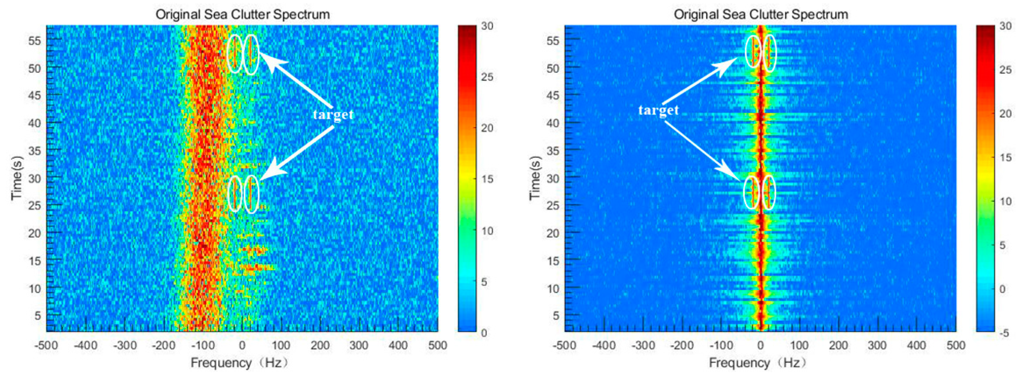
This section analyzes sea clutter suppression in different sea areas using a contrast analysis of the sea clutter obtained from the IPIX radar in the offshore and far-sea areas. Due to the height of the antenna frame (20 m in 1998), the distance between the point where the data are collected and the antenna is inversely proportional to the angle of the incident wave. That is, sea clutter under different sea areas can be regarded as being under different scraping angles (of course, distance also affects the amplitude of the received signal, but the IPIX radar compensates for the received gain by adjusting the voltage on the variable attenuator when receiving signals from the far sea areas). We use the IPIX radar data from 1998. Since the weather, wind, and wave information is incomplete, to ensure the same significant wave height, we select two sets of data close to the same day for analysis. The data of the offshore area were selected from the data collected by the sixth range gate of the 206th experiment in 1998. The distance from the antenna was 3051 m, and the ground angle was about 0.327°. The data of the far-sea area were selected from the data collected by the sixth range gate of the 214th experiment in 1998. The distance from the antenna was 26,151 m, and the ground angle was about 0.044°. Since the distance sampling point of the range gate was 60,000 (60 s) in 1998, the number of single movement points of the window was changed to 512 points (about 0.5 s), the virtual signal was added at 22.5–27.5 and 47.5–52.5 s, and the frequency point was still ±20 Hz. The time–frequency images in the offshore and far-seas areas are shown in Figure 8.
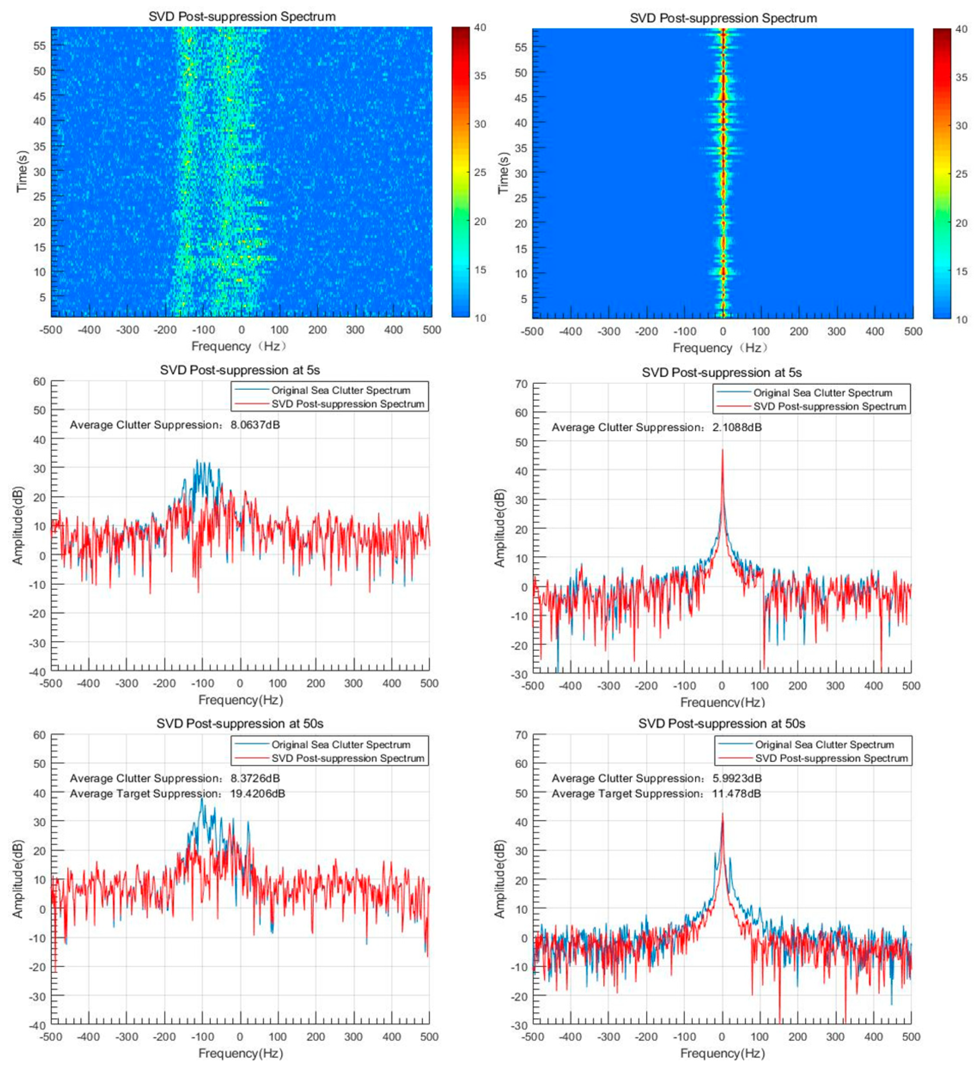
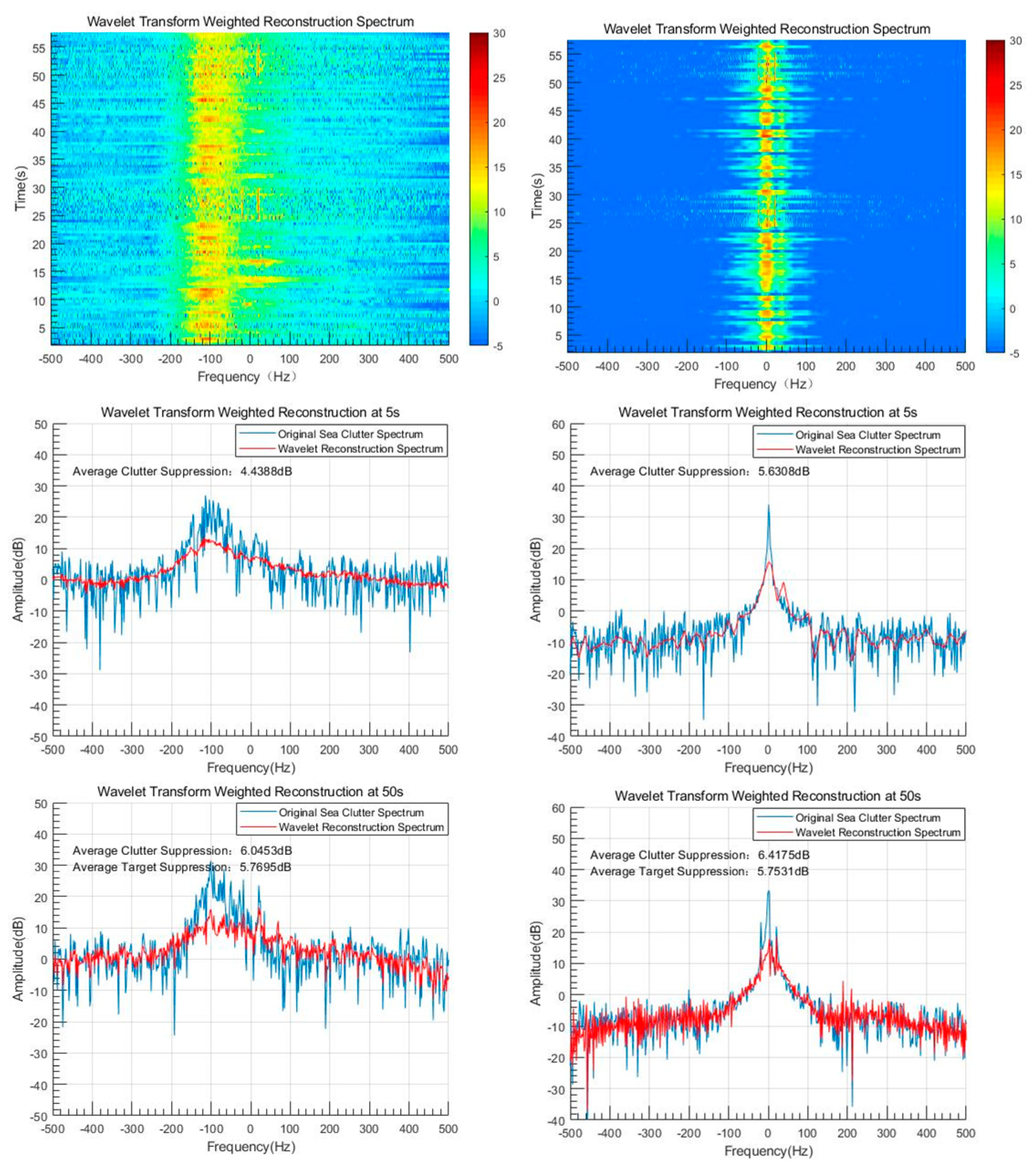
It can be seen that in the offshore area, the spectrum of the main component of the sea clutter is more broadened, while the spectrum of the main component of the sea clutter in the far sea area is narrow, and the spectrum of the strong component of the sea clutter in the offshore area can be found farther from the zero frequency. The sea clutter spectrum in the far-sea area is almost symmetric with about zero frequency. This is because the IPIX radar data in the far-sea area do not contain “H”-transmitted polarization. The suppression time–frequency images of each method were made separately, and the spectrograms before and after the suppression at different times were extracted. The extracted time is 50 s (with virtual target) and 5 s (without virtual target and for comparison) before and after the suppression of the spectrum comparison map while calculating the average suppression amplitude of the main components of the clutter and the suppression range of the target frequency, as shown in Figure 9, Figure 10, Figure 11 and Figure 12.
The cycle number of the root cycle cancellation in the offshore area is 60 times. When the spectrum of the suppression clutter is greatly widened, the loop cancellation has almost no effect and will suppress the target signal instead. Since the spectral broadening of the main component of the clutter in the far-sea area is narrow, the number of cyclic cancellations is chosen to be 10. Given a narrow spectrum of clutter, the suppression of cyclic cancellation is still good. Since the cyclic cancellation method mainly eliminates the harmonic peaks with high amplitude in the frequency domain, it can be clearly seen that the two virtual targets that are obviously symmetric in the frequency domain at 50 s are first suppressed. At the same time, it can be seen that the root cycle cancellation method has almost zero suppression at zero frequency. It can be concluded that the root loop cancellation method has a much weaker suppression effect when the main components of the clutter are broadened. When the target frequency is significantly symmetrical around the zero frequency, its ability to retain the target is worse.
The parameters for SVD suppression are the same as those in the previous section. It can be seen that the strong clutter components in the offshore area are almost suppressed, but in the far-sea area, the main clutter component has almost no suppression effect in the frequency domain close to or equal to zero. It can also be found that in the far-sea area, since the added virtual target is very similar to the first-order Bragg peak, SVD suppresses both of the symmetrical virtual targets. It can be concluded that SVD has a lesser suppression effect when the main components of the clutter, like the far-sea area, are small and symmetrical with respect to the zero frequency. When the target frequency is obviously symmetrical around the zero frequency, its ability to retain targets is worse.
It can be seen from the above figure that if the wavelet scale of the extracted frequency points is not much different from that of other frequency points in both the offshore and far-sea areas, the spectrum of the main components of the sea clutter will not only be suppressed but will be smoothed. Wavelet weighted reconstruction can achieve the effect of retaining the target and suppressing the clutter when the target is not hidden in the clutter, but the SNR cannot be improved when the target is hidden. It can be concluded that wavelet weighted reconstruction is less effective in suppressing clutter when the difference between the target spectrum and the clutter spectrum wavelet scale is small; thus, wavelet weighted reconstruction cannot simultaneously process two or more separated targets in the spectrum.
It can be seen from the above figure that EMD reconstruction can achieve good results in suppressing clutter and retaining targets in both near- and far-sea areas. It can be clearly seen from the figure that the frequency-suppression point of the target is about 1 dB, and the frequency of the main component of the clutter is much larger than 1 dB, so the effect of improving the SNR can be achieved. It can be concluded that the EMD reconstruction method can achieve a better suppression of clutter, superior retention of signals, and greater improvement of the SNR for known target information. Moreover, when the main components of the clutter in high sea conditions and offshore areas are widely spread in the frequency domain, we can obtain better suppression effects.
4. Statistical Analysis Based on IPIX Radar Data
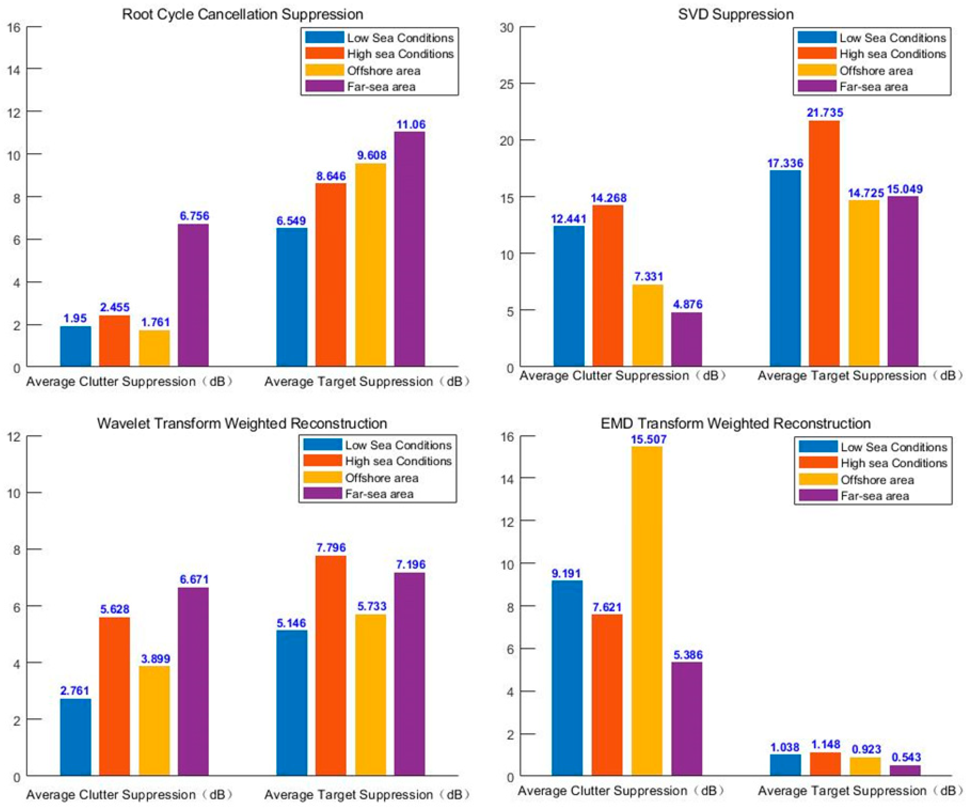
To avoid generality, we selected a small amount of data for statistical analysis under different sea conditions and different sea areas. The high-sea-state data were selected from all the range gate data collected in the 17th, 18th, and 19th experiments in 1993 (42 sets of data). The significant wave height was more than 2 m at the time of data collection, and the distance between the range gate and the antenna was 2574–5670 m. The low-sea-state data were collected from all the range gate data collected in the 25th, 26th, and 30th experiments in 1993 (42 sets of data). The significant wave height was about 1 m at the time of data collection, and the distance between the range gate and the antenna was 2574–2769 m. The data of the offshore area were selected from the first 25 range gates (50 sets of data) of the 207th and 209th experiments in 1998. The wind and wave conditions were unknown when the data were collected. The distance between the range gates and the antenna was between 2901 and 3621 m. The ground angle was about 0.316°–0.395°. To ensure that the wind and wave conditions in the far-sea area are similar to those in the offshore area, the data for the same day are selected (i.e., the data collected by the first 25 distance gates of the 214th and 215th experiments in 1998 (50 sets of data)). The distance between the range gate and the antenna is between 26,001 and 26,721 m, and the ground angle is about 0.043°–0.044°. Assume that the amplitude of the spectrum before the unsuppressed clutter is greater than or equal to 15 dB (25 dB for SVD) in the main component of the clutter. We calculate the average suppression amplitude of the main components of the clutter and the average suppression amplitude of the target and count them in a histogram, as shown in Figure 13.
It can be seen from the figure that the root cycle cancellation method cannot effectively suppress the clutter when the echo signal of the sea clutter has strong component spectrum broadening. The suppression amplitude can reach 6 dB only when facing the echo signal with a small spectrum width in the far sea area. Although SVD can achieve better clutter suppression (just like root cycle cancellation), it cannot retain the two added symmetrical virtual signals. Wavelet weight reconstruction can achieve a better suppression effect in the high-sea-state and far-sea area, but it cannot correctly retain the added virtual target, which still cannot improve the SNR. EMD reconstruction has the best effect. The virtual signal is well preserved with around 1 dB of the average suppression in various situations. Moreover, in the low-sea-state and offshore data statistics, the suppression amplitude of the sea clutter’s strong component spectrum reaches about 10 dB, which achieves the effect of improving the SNR.
5. Conclusions
To improve radar’s ability to detect targets such as ships against a background of strong sea clutter, the IPIX radar dataset is used to compare and analyze the suppression effect of root cycle cancellation, singular-value decomposition (SVD) suppression, wavelet weight reconstruction, and empirical mode decomposition (EMD) reconstruction methods on sea clutter and virtual signals in four conditions: high-sea-state, low-sea-state, offshore areas, and far-sea areas. The main findings are as follows:
- In terms of the suppression effect of sea clutter, the four methods have certain inhibitory effects, among which, EMD has the best effect. In the case of offshore areas, the average suppression amplitude reaches 15.507 dB, while the root cycle cancellation method has the worst inhibition effect on the offshore area, at 1.761 dB.
- Regarding the retention of the target echo, only the EMD algorithm can achieve a better retention of the target, and the suppression of the target echo is always below 1.2 dB. Wavelet weight reconstruction, root cycle cancellation, and SVD suppression cannot retain the two added targets. The SVD algorithm is the worst, and the suppression target’s amplitude is above 14 dB.
- The root cycle cancellation method only achieves an average 6.756 dB clutter-suppression effect when the main component of the sea clutter spectrum is very narrow. Otherwise, the suppression is less than 1.5 dB. At the same time, it can be found that the root cycle cancellation method cannot retain the two added virtual targets in the spectrum. The average suppression range of the target is above 6.5 dB and reaches as much as 11.06 dB in the far-sea areas.
- The SVD algorithm can better suppress clutter, achieving an average of 14.268 dB clutter suppression in high sea conditions. However, its signal retention is the worst of the four methods. Its signal-suppression range is above 14.5 dB and reaches as much as 21.735 dB in high sea conditions.
- The performance of wavelet reconstruction is ordinary in suppressing sea-clutter components and retaining signals. The average suppression clutter amplitude is 2.761–6.671 dB, and the average suppression signal amplitude is 5.146–7.796 dB. Since the suppression effect on the target exceeds that on the clutter, the SNR cannot be improved.
- EMD reconstruction can not only greatly suppress the sea-clutter component but can also better preserve the signal component. The average suppression effect on sea clutter can reach more than 5 dB (15.507 dB in the offshore areas). The average suppression effect on the target does not exceed 1.2 dB, so the EMD algorithm can achieve the effect of improving the SNR.
- Note that for EMD weighted reconstruction, we need to determine where the target is in the spectrum and then extract the target’s reconstruction coefficients. However, this does not mean that the EMD (or wavelet) algorithm makes no sense, since we only need to determine the position of the target in the spectrum at a certain moment. If the radar detects a target with a background of weak sea clutter, we can find the target in the spectrum at this moment and extract the reconstruction coefficients we need. Since the EMD algorithm is adaptive, we can perform clutter suppression continuously and obtain more precise target parameters (the radial velocity of the target and the target location). In this way, even if subsequent clutter energy is stronger and the radar cannot detect the target, we can still use the EMD algorithm to suppress the clutter and extract the target parameters. Ultimately, the EMD algorithm can improve the ability of radar to detect and track targets such as ships against a background of strong sea clutter.
Author Contributions
M.L. and C.Z. conceived the idea and analyzed the results. C.Z. provided funding and supervised the study. M.L. wrote the main manuscript. C.Z. provided suggestions and comments and revised the manuscript.
Funding
This research was funded by the Hubei Provincial Natural Science Foundation of China for Distinguished Young Scholars with grant number 2019CFA054 and the Key Program of Equipment Pre-Research Field Foundation of China with grant number 61404130109.
Acknowledgments
The authors would like to gratefully thank the anonymous reviewers for their insightful and helpful. The authors would like to appreciate the usage of Intelligent PIxel processing X-band (IPIX) radar datasets.
Conflicts of Interest
The authors declare no conflict of interest.
References
- Borge, J.C.N.; Rodriguez, G.R.; Hessner, K. Inversion of Nautical Radar Images for Surface Wave Analysis. J. Atmos. Ocean. Technol. 2004, 21, 1291–1300. [Google Scholar] [CrossRef]
- Barrick, D.E.; Headriek, J.M.; Bogle, R.W.; Crombie, D.D. Sea backscatter at HF: Interpretation and Utilization of the echo. Proc. IEEE 1974, 62, 673–680. [Google Scholar] [CrossRef]
- Lipa, B.J.; Barrie, D.E. Extraction of sea state from HF radar sea echo: Mathematical theory and modeling. Radio Sci. 1986, 21, 81–100. [Google Scholar] [CrossRef]
- Gill, E. The Scattering of High Frequency Electromagnetic Radiation from the Ocean Surface: An Analysis Based on a Bistatic Ground Wave Radar Configuration. Ph.D. Thesis, Faculty of Engineering and Applied Science Memorial University of Newfoundland, St. John’s, NL, Canada, 1999; pp. 10–16. [Google Scholar]
- Khan, R.H. Ocean-clutter Model for High-Frequency Radar. IEEE J. Ocean. Eng. 1991, 16, 181–188. [Google Scholar] [CrossRef]
- Fan, L.; Chen, Z.; Chen, X.; Jin, X. S-band Radar Measurement of Correlation between Coastal Wave and Tide. JDCTA 2012, 19, 503–510. [Google Scholar]
- Skolnik, M.I. Radar Handbook, 3rd ed.; McGraw-Hill: New York, NY, USA, 2008. [Google Scholar]
- Barrick, D.E. First-order theory and analysis of MF/HF/VHF scatter form the sea. IEEE Trans. Antennas Propag. 1972, 20, 2–10. [Google Scholar] [CrossRef]
- Ji, Z.; Meng, X.; Zhou, H. Analyses of sea clutters in HF ground wave over-the-horizon radar. J. Syst. Eng. Electron. 2000, 22, 12–15. [Google Scholar]
- Root, B.T. HF Radar Ship Detection through Clutter Cancellation. In Proceedings of the National Radar Conference, Dallas, TX, USA, 14 May 1998; pp. 281–286. [Google Scholar]
- Root, B.T. HF-over-the-horizon Radar Ship Detection with Short Dwells Using Clutter Cancellation. Radio Sci. 1998, 33, 1095–1111. [Google Scholar] [CrossRef]
- Khan, R.; Power, D.; Walsh, J. Ocean Clutter Suppression for an HF Wave Radar. In Proceedings of the Canadian Conference on Electrical and Computer Engineering. Engineering Innovation: Voyage of Discovery. Conference Proceedings, Saint Johns, NL, Canada, 25–28 May 1997; pp. 512–515. [Google Scholar]
- Wang, J.; Kirlin, R.L. Improvement of High Frequency Ocean Surveillance Radar Using Subspace Methods Based on Sea Clutter Suppression. In Proceedings of the IEEE Proceedings on Sensor Array and Multichannel Signal Processing Workshop, Rosslyn, VA, USA, 6 August 2002; pp. 557–560. [Google Scholar]
- Poon, M.W.Y. A Clutter Suppression Scheme for High Frequency (HF) Radar. Master’s Thesis, Memorial University of Newfoundland, St. John’s, NL, Canada, 1991. [Google Scholar]
- Jangal, F.; Saillant, S.; Hélier, M. Ionospheric Clutter Cancellation and Wavelet Analysis. In Proceedings of the European Conference on Antennas and Propagation, Nice, France, 6–10 November 2006; pp. 1–6. [Google Scholar]
- Jangal, F.; Saillant, S.; Hélier, M. Ionospheric Clutter Mitigation Using One-dimensional or Two-dimensional Wavelet Processing. IET Radar Sonar Navig. 2009, 3, 112–121. [Google Scholar] [CrossRef]
- Huang, N.E.; Shen, Z.; Long, S.R.; Wu, M.C.; Shih, H.H.; Zheng, Q.; Yen, N.C.; Tung, C.C.; Liu, H.H. The Empirical Mode Decomposition and the Hilbert Spectrum for Nonlinear Nonstationary Time Series Analysis. Proc. R. Soc. Lond. A 1998, 454, 903–995. [Google Scholar] [CrossRef]
- Huang, N.E.; Zheng, S.; Steven, R.I. A new view of nonlinear water waves: The Hilbert spectrum. Annu. Rev. Fluid Mech. 1999, 31, 417–457. [Google Scholar] [CrossRef]
- Huang, N.E. A new spectral representation of earth-quake data: Hilbert spectral analysis of station TCU 129, Chi-Chi, Taiwan, 21 September 1999. BSSA 2001, 91, 1310–1338. [Google Scholar]
- Loh, C.H.; Wu, T.C.; Huang, N.E. Application of the empirical mode decomposition Hilbert spectrum method to identify near-fault ground motion characteristics and structural responses. BSSA 2001, 91, 1339–1357. [Google Scholar] [CrossRef]
- Vincent, H.T.; Hu, S.L.J.; Hou, Z. Damage Detection Using Empirical Mode Decomposition Method and a Comparison with Wavelet Analysis. In Proceedings of the 2nd International Workshop on Structural Health Monitoring, Stanford, CA, USA, 8–10 September 2000; pp. 891–900. [Google Scholar]
- Nikoiaos, P.P. Advanced time–frequency analysis applications in earth-quake engineering. Seism. Des. Anal. Struct. 2004, 2002–2003, 23–24. [Google Scholar]
- Veltcheva, A.D.; Soares, C.G. Identification of the components of wave spectra by the Hilbert Huang transform method. Appl. Ocean Res. 2004, 26, 1–12. [Google Scholar] [CrossRef]
- Xiao, C.; Cha, H.; Xia, D. Sea Clutter Characteristics Analysis and Target Detection Based on HHT. In Proceedings of the International Conference on Consumer Electronics, Communications and Networks (CECNet), XianNing, China, 16–18 April 2011; pp. 694–697. [Google Scholar]
- Jangal, F.; Mandereau, F. Morphological Operator and Empirical Mode Decomposition for Clutter Mitigation. In Proceedings of the OCEANS, Quebec City, QC, Canada, 15–18 September 2008. [Google Scholar]
- Tanaka, T.; Mandic, D.P. Complex Empirical Mode Decomposition. IEEE Signal Process. Lett. 2007, 14, 101–104. [Google Scholar] [CrossRef]
- Haykin, S. The Dartmouth Database of IPIX Radar [EB/OL]. (2001-06-08) [2007-5-23]. Available online: http://soma.ece.mcmaster.ca/ipix/dartmouth/ (accessed on 20 November 2019).
Figure 1.
Time–frequency image.

Figure 2.
Spectrum of sea clutter at 10 s.

Figure 3.
Adding virtual targets to low sea conditions (left) and high sea conditions (right).

Figure 4.
Root cycle cancellation suppression under low sea conditions (left) and high sea conditions (right).
Figure 4.
Root cycle cancellation suppression under low sea conditions (left) and high sea conditions (right).

Figure 5.
Singular-value decomposition (SVD) suppression under low sea conditions (left) and high sea conditions (right).
Figure 5.
Singular-value decomposition (SVD) suppression under low sea conditions (left) and high sea conditions (right).

Figure 6.
Wavelet transform weighted reconstruction under low sea conditions (left) and high sea conditions (right).
Figure 6.
Wavelet transform weighted reconstruction under low sea conditions (left) and high sea conditions (right).

Figure 7.
Empirical mode decomposition (EMD) reconstruction under low sea conditions (left) and high sea conditions (right).
Figure 7.
Empirical mode decomposition (EMD) reconstruction under low sea conditions (left) and high sea conditions (right).

Figure 8.
Adding virtual targets to the offshore area (left) and far-sea area (right).

Figure 9.
Root cycle cancellation suppression in the offshore area (left) and far-sea area (right).

Figure 10.
SVD suppression in the offshore area (left) and far-sea area (right).

Figure 11.
Wavelet weighted reconstruction in the offshore area (left) and far-sea area (right).

Figure 12.
EMD reconstruction in the offshore area (left) and far-sea area (right).

Figure 13.
Statistics of the inhibition effects of the four methods under different conditions.


Table 1.
Main parameters of the realistic Intelligent PIxel processing X-band (IPIX) radar.
| Radar Parameter | Typical Value |
|---|---|
| Transmitting frequency (RF_frequency) | 9.39 GHz |
| Pulse repetition frequency (PRF) | 0–20 kHz (typical value is 1000 Hz) |
| Pulse width (pulse_length) | 20–5000 ns (typical value is 200 ns) |
| Antenna maximum gain (antenna_gain) | 45.7 dB |
| Polarization mode | HH/VV/HV/VH (linear polarization) |
| Antenna height | 30 m (1993), 20 m (1994) |
| Distance resolution (radar_elev) | 30 m |
© 2019 by the authors. Licensee MDPI, Basel, Switzerland. This article is an open access article distributed under the terms and conditions of the Creative Commons Attribution (CC BY) license (http://creativecommons.org/licenses/by/4.0/).
Share and Cite
MDPI and ACS Style
Lv, M.; Zhou, C. Study on Sea Clutter Suppression Methods Based on a Realistic Radar Dataset. Remote Sens. 2019, 11, 2721. https://doi.org/10.3390/rs11232721
AMA Style
Lv M, Zhou C. Study on Sea Clutter Suppression Methods Based on a Realistic Radar Dataset. Remote Sensing. 2019; 11(23):2721. https://doi.org/10.3390/rs11232721
Chicago/Turabian StyleLv, Mingjie, and Chen Zhou. 2019. "Study on Sea Clutter Suppression Methods Based on a Realistic Radar Dataset" Remote Sensing 11, no. 23: 2721. https://doi.org/10.3390/rs11232721
Note that from the first issue of 2016, this journal uses article numbers instead of page numbers. See further details here.