Mapping Water Surface Elevation and Slope in the Mississippi River Delta Using the AirSWOT Ka-Band Interferometric Synthetic Aperture Radar

Abstract

AirSWOT is an airborne Ka-band synthetic aperture radar, capable of mapping water surface elevation (WSE) and water surface slope (WSS) using single-pass interferometry. AirSWOT was designed as a calibration and validation instrument for the forthcoming Surface Water and Ocean Topography (SWOT) mission, an international spaceborne synthetic aperture radar mission planned for launch in 2022 which will enable global mapping of WSE and WSS. As an airborne instrument, capable of quickly repeating overflights, AirSWOT enables measurement of high frequency and fine scale hydrological processes encountered in coastal regions. In this paper, we use data collected by AirSWOT in the Mississippi River Delta and surrounding wetlands of coastal Louisiana, USA, to investigate the capabilities of Ka-band interferometry for mapping WSE and WSS in coastal marsh environments. We introduce a data-driven method to estimate the time-varying interferometric phase drift resulting from radar hardware response to environmental conditions. A system of linear equations based on AirSWOT measurements is solved for elevation bias and time-varying phase calibration parameters using weighted least squares. We observed AirSWOT WSE uncertainty of 12 cm RMS compared to in situ water level measurements when averaged over an area of 0.5 km${}^2$ at incidence angles below ${15}^{\circ }$. At higher incidence angles, the observed AirSWOT elevation bias is possibly due to residual phase calibration errors or radar backscatter from vegetation. Elevation profiles along the Wax Lake Outlet river channel indicate AirSWOT can measure WSS over a 24 km distance with uncertainty below 0.3 cm/km, 8% of the true water surface slope as measured by in situ data. The data analysis and results presented in this paper demonstrate the potential of AirSWOT to measure water surface elevation and slope within highly dynamic and spatially complex coastal environments.

1. Introduction

Quantifying and monitoring the volume and distribution of water is important, particularly as climate change and other factors cause additional stress to Earth’s limited water resources [1,2]. Accurate measurements of these water resources are important in planning for both overabundance and dearth of water, as in floods and droughts, respectively. Rivers and lakes are particularly important due to their ease of access and role in flood hazards. Unfortunately, in situ data regarding surface water is incomplete or unavailable in many parts of the world [3]. In response to this limitation, there has been an increased focus on using data from satellites to measure rivers and lakes [4]. Remote sensing measurements of water surface elevation (WSE) and water surface slope (WSS) can be used to estimate important hydrological parameters such as river discharge and fresh water storage at regional and global scales [4,5].

Radar and radar altimetry, in particular, have proven to be valuable tools for mapping discharge, WSE, WSS, and relative water level change from space, as shown by many previous studies, for example, in [6,7,8,9,10,11,12,13]. However, traditional radar altimetry has limited coverage area and temporal resolution [4]. While repeat-pass interferometric synthetic aperture radar (InSAR) [14] is often used to estimate relative water level change in large inundated wetlands [8,9,11], low interferometric coherence observed over open water surfaces, without vegetation, make accurate estimates of WSE impossible [4]. In order to estimate WSE in open water areas at a high spatial and temporal resolution, a specialized instrument is required, such as the forthcoming Surface Water and Ocean Topography (SWOT) mission. The SWOT mission will enable WSE and WSS to be mapped globally from space [4,15,16,17,18]. SWOT is being jointly developed by the National Aeronautics and Space Administration (NASA) and the Centre National D’Etudes Spatiales (CNES) with contributions from the Canadian Space Agency and United Kingdom Space Agency. SWOT will provide fine-resolution observations of WSE and WSS over inland rivers and lakes, and coarser resolution observations over the ocean [15]. More details on the SWOT mission can be found, for example, in [4,15,16,17,18,19,20,21,22].

NASA initially developed AirSWOT, an airborne Ka-band InSAR instrument, to calibrate and validate SWOT [23]. Early studies had demonstrated the feasibility and potential of Ka-band InSAR for mapping water surfaces, using both ground-based [24] and airborne radar experiments [25,26]. Recent studies have demonstrated the capabilities of AirSWOT to measure rivers and lakes [27,28,29,30,31]. Altenau et al. [27] used AirSWOT data to measure WSE, WSS, and estimate discharge [28] along the Tanana River, Alaska, USA. They reported WSE root mean square error (RMSE) of 9.0 cm over 1 km${}^2$ areas, WSS RMSE of 1.0 cm/km along 10 km river reaches, and discharge RMSE around 10–20%. Pitcher et al. [29] used AirSWOT to map WSE for rivers and lakes in the Yukon Flats Basin, Alaska, reporting WSE RMS errors between 8 to 15 cm over rivers and 21 cm over lakes. Similarly, Tuozzolo et al. [30] used AirSWOT data to estimate WSE, WSS, and river discharge over the Willamette River in Oregon, USA, reporting WSE and WSS RMSE of 11.6 cm and 3.2 cm/km, respectively, and discharge error of 10 to 31% depending on discharge algorithm and accurate prior estimate of mean annual discharge. While these uncertainties are slightly higher than that of Altenau et al. [27,28] or Pitcher et al. [29], Tuozzolo et al. noted the Willamette is a thinner river, requiring smaller averaging windows (i.e., less pixels). Appropriate methods for averaging and filtering of AirSWOT data enable accurate estimation of WSE and WSS in spite of the noise in AirSWOT measurements [27,28,29,30,31].

There have been studies of coastal areas using simulated SWOT data [32,33], but its ability to measure high frequency and fine scale hydrological processes is limited by the 21 day repeat orbit, which results in a revisit period of 3–12 days depending on latitude [19,22]. In comparison, AirSWOT can measure WSE and WSS multiple times per day to, for example, capture different parts of the tidal cycle. Coastal deltas, in particular, are threatened by relative sea level rise (RSLR), declining sediment input due to reservoir construction, anthropogenic land use change, and the increasing occurrence and intensity of storms [34,35]. The Mississippi River Delta has the seventh largest river discharge in the world [36] and improving our understanding of the hydrology across the Mississippi River Delta is needed to assess its vulnerability and resilience. This study demonstrates the potential of AirSWOT to perform accurate WSE and WSS measurements within coastal regions such as river deltas or coastal wetlands. We use AirSWOT data collected on 8 May, 9 May, and 11 May of 2015 in the Wax Lake and Atchafalaya river deltas (tributaries of the Mississippi River), as well as the surrounding wetlands around Terrebonne Bay (Figure 1). This study also serves as a preliminary investigation for Delta-X, a NASA-funded Earth Ventures mission focused on delta processes. Delta-X (https://deltax.jpl.nasa.gov/) will use several airborne remote sensing instruments, including AirSWOT, in order to study the relative contribution of vegetation and channel-network to soil accretion rates. We also seek to demonstrate AirSWOT’s capabilities to generate accurate WSE and WSS measurements supporting potential implementations of the Delta-X framework to other study areas.

This paper is structured as follows. We introduce the data used in this study in Section 2 and present an overview of the AirSWOT instrument in Section 2.1. The in situ data collection and processing is discussed in Section 2.2. We introduce the operational interferometric phase calibration methodology in Section 3.1, followed by the proposed calibration approach adapted to these coastal landscapes. In Section 3.2 we describe the filtering and averaging methodology we used to estimate WSE from the noisy AirSWOT data. The results are presented in Section 4. We present and discuss the AirSWOT WSE results in Section 4.1. In Section 4.2, we show relative WSE estimation over time. AirSWOT-derived profiles of WSE and WSS in the Wax Lake Outlet river channel are shown in Section 4.3. Our conclusions are discussed in Section 5.

2. Data

2.1. AirSWOT Overview

AirSWOT consists of three main instruments. The primary instrument is called the Ka-band SWOT Phenomenology Airborne Radar, or KaSPAR. KaSPAR is the interferometric synthetic aperture radar used by AirSWOT to measure surface water levels. The other two instruments are an Applanix POSAV 610 integrated GNSS and IMU (global navigation satellite system and inertial measurement unit), and a Cirrus color infrared digital camera system. The GNSS and IMU are used to precisely track the aircraft position and remove the effects of aircraft motion and attitude on the radar data. The digital camera can be used to map the extents of surface water in cloud-free conditions (e.g., [37]). In this study the camera was not installed, and instead, we used a pre-existing land cover mask generated from Sentinel-2 data by Thomas et al. [38] to delineate land and water.

KaSPAR uses six different antennas to collect interferometric data in a variety of imaging modes and with different cross-track and along-track spatial baselines. In this study, we focus on data from the KaSPAR outer swath mode, which has incidence angles ranging nominally between 4–${25}^{\circ }$. In practice, large errors are often observed at the edges of this range, such that the usable swath is generally smaller (see Section 4.1).

The main characteristics of AirSWOT and the AirSWOT outer swath data are shown in

Table 1. Summary of AirSWOT characteristics for the outer swath mode.

Aircraft Type	Beechcraft Super King Air B200
Aircraft Altitude	≈8900–9000 m
Center Frequency	35.75 GHz
Wavelength	0.84 cm
Polarization	VV
Nominal Incidence Angle Range	4–${25}^{\circ }$
Nominal Swath Width	4 km
Effective Swath Width	3 km
Azimuth Processing Beamwidth	$2^{\circ }$
Pulse Repetition Frequency	1729 Hz
Range Bandwidth (Transmitted)	80 MHz
Slant Range Resolution	≈2 m
Along-Track Looks	50
Along-Track Baseline	50 cm
Cross-Track Baseline	50 cm

. In addition to the outer swath mode, KaSPAR has an inner swath mode with incidence angles ranging between 0–$7^{\circ }$, designed to more closely reflect the range of incidence angles that will be collected by SWOT. Compared to the outer swath mode, the inner swath mode uses a smaller cross-track antenna beamwidth and a higher range bandwidth of 450 MHz, yielding a range resolution of ≈ 40 cm (compared to ≈ 2 m for the outer swath). However, for this study, we focus exclusively on the outer swath mode which, advantageously, covers a wider surface swath.

AirSWOT uses both cross-track and along-track interferometry to accurately measure water surface elevation. Cross-track interferometry is sensitive to the vertical position of radar scatterers in a scene [14], allowing cross-track interferometry to be used to estimate elevation. However, using cross-track interferometry alone to estimate water surface elevation would result in biased WSE estimates. This is because water is a moving target, and the velocity of water in the direction of the radar line of sight will cause a doppler shift, which changes the interferometric phase [39,40]. Along-track interferometry can be used to estimate the motion of the water scatterers [39,40]. AirSWOT uses along-track interferometry to estimate the doppler shift introduced by water motion, and then compensate for the effects of that doppler shift in the cross-track interferograms. The cross-track and along-track interferometric data are combined into a motion-compensated cross-track interferogram, from which the water surface elevation can be estimated with the effects of the motion-induced interferometric phase bias removed.

Since KaSPAR is a single-pass multi-static InSAR system, the cross-track and along-track data are collected simultaneously. For the outer swath mode, KaSPAR transmits using one antenna and receives using three antennas (one of which is the same as the transmit antenna), forming two interferometric baselines. The first baseline is in the cross-track direction, while the second baseline is primarily along-track, with a small cross-track component. More details on the KaSPAR instrument can be found in [23].

2.2. In Situ Water Level Data

We used in situ water level measurements to calibrate and validate the AirSWOT estimates. Several stations within the study regions are managed by the United States Geological Survey (USGS), the National Oceanic and Atmospheric Administration (NOAA), and the Coastwide Reference Monitoring System (CRMS) [41]. These organizations publicly distribute their data online. We also used a Louisiana State University (LSU) dataset of in situ water level collected within the Wax Lake Delta, on Mike Island. A summary of the USGS, NOAA, CRMS, and LSU water level stations used in this study are shown in

Table 2. Summary of the in situ water level stations used in this study. The first two stations listed in the table were used as GCPs in the AirSWOT calibration procedure, while the remaining stations were kept independent for validation purposes.

Station Name	Org.	Latitude (${}^{\circ }$)	Longitude (${}^{\circ }$)	Vertical Datum Conversion
Wax Lake Outlet at Calumet	USGS	29.698	−91.373	Published Offset
Caillou Bay	USGS	29.078	−90.871	Published Offset
Avoca Island Cutoff	USGS	29.539	−91.246	Published Offset
Mike Island	LSU	29.496	−91.444	Surveyed Offset
Eugene Island	NOAA	29.367	−91.383	NOAA VDatum
Amerada Pass	NOAA	29.450	−91.338	NOAA VDatum
0303	CRMS	29.241	−91.069	N/A
0305	CRMS	29.390	−91.198	N/A
0311	CRMS	29.214	−90.792	N/A
0329	CRMS	29.480	−91.105	N/A
0345	CRMS	29.171	−90.762	N/A
0347	CRMS	29.161	−90.701	N/A
0354	CRMS	29.332	−91.009	N/A
0369	CRMS	29.295	−90.695	N/A
0374	CRMS	29.157	−90.793	N/A
0376	CRMS	29.124	−90.857	N/A
0377	CRMS	29.232	−91.007	N/A
0383	CRMS	29.208	−90.948	N/A
0396	CRMS	29.343	−90.886	N/A
0421	CRMS	29.172	−90.824	N/A
0434	CRMS	29.320	−90.733	N/A
0464	CRMS	29.518	−91.387	N/A
0479	CRMS	29.524	−91.449	N/A
2785	CRMS	29.503	−91.040	N/A
4455	CRMS	29.259	−90.943	N/A
4782	CRMS	29.665	−91.442	N/A
6038	CRMS	29.605	−91.353	N/A
6304	CRMS	29.420	−91.279	N/A

. In the table, the first two stations (Calumet and Caillou Bay) were used in the AirSWOT calibration procedure (Section 3.1). The remaining stations were used as independent validation of the AirSWOT water level estimates. In the table, the approximate geographic position of each station is listed.

For this study, we used NAVD88 as the common vertical datum to compare between the remote sensing and in situ data. In the last column of the table, we list how the in situ water levels with respect to the gauge datums were converted to the NAVD88 vertical datum (using the GEOID12B geoid model). The USGS stations were easy to convert, as each USGS station used in this study had a published offset with respect to NAVD88. There were two USGS stations within our study area (at Crewboat Channel and Caillou Lake) which did not have publicly available datum information (or, in the case of Caillou Lake, had datum information using an unknown geoid model). These stations were excluded from the analysis. While the Calumet station has a published vertical offset of −17.07 cm with respect to NAVD88, this did not explain a bias we initially observed between AirSWOT and the station. After inquiring with the USGS Baton Rouge Office we learned the datum offset was with respect to an older geoid model (GEOID99) when the Calumet station was last surveyed in 1996 [42]. We converted the Calumet water levels from GEOID99 to GEOID12B using the publicly available NOAA VDatum software tool [43] and determined an additional offset of −20.7 cm.

Water levels from the two NOAA water level stations are published with respect to local tidal datums and were converted to NAVD88 using NOAA VDatum [43]. VDatum reports the uncertainty associated with this datum conversion, which was 15.7 cm for both the Eugene Island and Amerada Pass stations.

The LSU Mike Island water level gauge had its datum surveyed using real-time kinematic (RTK) positioning in February of 2017. We assume sinking of the water level gauge to be negligible between the gauge and AirSWOT survey dates.

The CRMS stations report their water levels in NAVD88, with the geoid model used for each water level sample included in the data. All of the CRMS data used in this study were already in the GEOID12B geoid model, therefore no vertical datum conversion was required for these data.

A first assessment of AirSWOT WSE estimates revealed conflicting behaviours between CRMS and non-CRMS stations. While the USGS and NOAA stations tend to be located in large river channels or in large areas of open water, many CRMS stations are located in small distributary channels often located near emergent wetland vegetation. The LSU station was located near the middle of Mike Island, which was flooded during the time period of this study. Therefore, we consider separately the non-CRMS and CRMS stations throughout this paper, particularly when discussing the results in Section 4.

Figure 1 shows an overview map of the study area, with the locations of the in situ water level stations superimposed on a map of the calibrated AirSWOT elevation data, which should not be confused with a map of WSE. The map represents the elevation estimated from the AirSWOT interferometric phase, which is biased compared to the true WSE in vegetated areas. In order to estimate WSE from the AirSWOT elevation products, additional filtering and averaging is required (Section 3.2). The stations are colored according to their source. The two stations used as GCPs for AirSWOT calibration (Calumet and Caillou Bay) are annotated with their names. We chose to use Calumet and Caillou Bay as the calibration stations because they are located near the corners of the study area and are representative of the high and low ends of the observed water level range, respectively.

Figure 2 shows a map zoomed in more closely on the Wax Lake and Atchafalaya River deltas. In this map, some of the stations used for validation (Avoca Island Cutoff, Mike Island, Eugene Island, Amerada Pass, and CRMS 0479) are annotated with their names.

Unfortunately, the NOAA stations at Eugene Island and Amerada Pass were located outside the bounds of the AirSWOT data coverage. For the purposes of our analysis, we treated these stations as if they were located within the coverage area of nearby AirSWOT flight lines by creating a “virtual location” for each station. In Figure 2, the true location of each NOAA station is shown in dark blue, while the virtual location used in our analysis is shown in light blue. For Amerada Pass, the virtual location is approximately 2.3 km from the true position, and has been moved from a small deltaic river channel into the open water outside the delta. This is also helpful because vegetation near river channels can introduce biases into the AirSWOT water level estimates (as discussed in Section 4.1). The distance between the true and virtual locations for the Eugene Island station is 3.2 km, with the virtual location lying inside the nearest AirSWOT swath. We justify this by noting that the Eugene Island and Amerada Pass stations are located in the Atchafalaya Delta, close to the ocean, where it is expected the WSS is relatively flat compared to the steeper upstream WSS. To determine the potential WSE error introduced by moving these stations, we calculated the WSS between the Eugene and Amerada stations from the in situ data, finding that the WSS varied between 0.04 and 0.88 cm/km during the AirSWOT acquisition period spanning 3 days. By moving the Eugene Island station by 3.2 km, the WSS values may result in a change in WSE between 0.13 and 2.83 cm. For the Amerada Pass station, the change in WSE is between 0.09 and 2.02 cm. This change in WSE between the original and shifted station locations is significantly smaller than the elevation uncertainty of the stations’ vertical datum conversion (15.7 cm) or the AirSWOT data itself (as shown in Section 4).

3. Methods

3.1. AirSWOT Phase Calibration Procedure for Coastal Wetlands

Phase calibration is a critical part of InSAR processing [44,45,46,47]. In the case of AirSWOT, the phase calibration consists of estimating unintended differential phase delays between radar channels in the KaSPAR instrument. These differential phase delays cause an InSAR phase bias if not removed. An InSAR phase bias introduces a cross-track slope in the measured elevations, because the relationship between interferometric phase and elevation varies with incidence angle [14]. For AirSWOT, this phase bias varies with time—due in part to changes in instrument temperature—introducing a time-varying cross-track elevation slope if not estimated and removed. This phase drift was found to differ between flights and must be estimated from the InSAR data itself.

The KaSPAR instrument contains internal calibration loops that were designed to measure the phase delays between certain points within the radar hardware. Unfortunately, in practice these calibration loops are insufficient to fully characterize the observed phase drift, leaving residual phase calibration errors. The AirSWOT processor therefore uses the calibration loops to provide an initial estimate of the differential phase delays, which are then refined using data-driven methods. Note that due to hardware and platform differences between KaSPAR and KaRIn (Ka-band Radar Interferometer, the primary instrument on SWOT), the phase calibration methods we discuss here are only applicable to KaSPAR. For information on SWOT calibration plans, see [48].

The operational AirSWOT phase calibration procedure fits a set of phase correction coefficients for each AirSWOT flight line: a constant phase bias and, optionally, a phase bias term that is a linear function of along-track distance. The linear phase bias term is only used for flight lines where the phase correction changes significantly over the course of the flight line. The phase corrections usually change rapidly at the beginning of each flight, then gradually become more stable.

In the operational phase calibration, the phase correction coefficients are estimated using AirSWOT pixels over stationary land areas. If a high resolution digital elevation model (DEM) is available, DEM pixels over non-vegetated stationary land areas with high interferometric coherence can be used as ground control points (GCPs). The GCPs are used to estimate the phase correction needed for AirSWOT to match the GCP elevation. The estimated phase correction is added to the interferometric phase to produce a calibrated AirSWOT interferogram. If a high resolution DEM is not available, the phase correction parameters can be fitted by minimizing the elevation difference between repeat AirSWOT measurements of the same stationary surface (typically land). Essentially, pixels within these stationary surfaces are used as tie points in order to calibrate the interferometric phase of multiple AirSWOT flight lines within the overlapping area.

Either method (GCP or tie point) can be represented as a system of linear equations, solved in the AirSWOT processing chain using a weighted least squares method. However, these methods work best with the presence of bare ground areas within the study area, without significant vegetation or topography.

In vegetated areas, the AirSWOT elevation measurements are biased above ground level. The magnitude of this bias varies as a function of vegetation structure and incidence angle. This is because the microwave penetration depth within the vegetation canopy depends on incidence angle (e.g., [49,50,51]). This implies vegetated areas cannot be reliably used as either GCPs or tie points. Locations with severe topography also cannot be used, because elevation measurements from varying viewing geometries for the same location may differ as a result of foreshortening and layover [14]. The effects of foreshortening and layover in AirSWOT and SWOT data are significant due to the steep incidence angles at which these instruments operate [20,33].

We developed a new phase calibration procedure better suited to coastal wetland environments where stationary and non-vegetated land areas may be scarce or nonexistent. This new approach uses AirSWOT water surface measurements (i.e., only open water pixels) rather than land to generate a system of linear equations. The calibration approach is based on two objectives: (i) remove cross-track slopes by minimizing slopes in areas where cross-track WSS are expected to be small; and (ii) Remove absolute WSE errors by minimizing the difference between the AirSWOT WSE and in situ water level data which serve as ground control points (GCPs). The use of external elevation data for calibration of elevations estimated from radar interferometry is a standard practice [52,53], helping to account for errors in the platform position or baseline calculations, which can impact the accuracy of DEMs generated from radar interferometry. The main difference with our method is that the GCPs represent WSE rather than land elevations. Since WSE varies over time, when using the in situ WSE to calibrate AirSWOT, we interpolate the in situ WSE to the AirSWOT acquisition time using linear interpolation between the two closest measurements.

The effect of the AirSWOT phase calibration procedure on the data is illustrated in Figure 3. The original WSE measurement including the original phase drift estimate is compared to the new phase-calibrated measurements. The original WSE used a phase calibration method where the AirSWOT elevations over land were fitted to the SRTM DEM, creating a significant cross-track elevation slope, presumably due to vegetation-related biases, errors in the DEM, and a lack of land targets. To demonstrate the difference between the original calibration and our new method, we selected an area of water southwest of the Wax Lake Delta where cross-track slope should be minimal over the AirSWOT swath. In the original data the cross-track elevation slope is equal to almost 100 cm/km across the AirSWOT radar swath, an unrealistically large WSS value in this area (see Section 4.3). A higher resolution and more accurate DEM may improve those results, but the vegetation related biases would remain an issue. Here, we propose an algorithm that does not rely on a DEM. The cross-track slope is mitigated with the new calibration procedure as shown in Figure 3b.

To preserve the true water surface slopes in the channels of the Wax Lake and Atchafalaya river systems, we fit the AirSWOT elevation profile across non-river open water surfaces to the local NAVD88 geoid (with a fitted elevation bias that varies between flight lines, to account for tidal changes). The water mask was used to select large water bodies that are not channels, as the latter may exhibit significant slopes unrelated to the geoid. A map of this calibration mask is shown in Figure 4, where black shading denotes areas that were excluded from the calibration procedure. This includes the Wax Lake and Atchafalaya rivers and deltas, as well as the areas that were classified as land in the a priori water mask. While the assumption that the water surface is locally flat with respect to the geoid in these areas may cause phase calibration errors (e.g., if the WSS is significant), we demonstrate the assumption is reasonable by showing strong agreement between calibrated AirSWOT WSEs and in situ data as shown in Section 4.

When fitting the phase correction coefficients, we fit either a zero order (constant phase correction) or first order (linear phase correction as a function of along-track distance) correction for each flight line. To fit these phase correction coefficients, the equation linking the observed AirSWOT elevation bias to the phase correction can be written as follows for a single AirSWOT image pixel:

$$\frac{dh}{d\varphi }{\varphi }_0+\Delta h=h_{AirSWOT}-h_{NAVD88}$$

(1)

$\frac{dh}{d\varphi }$ is the conversion factor between elevation and interferometric phase for that pixel, which can be calculated using knowledge of the AirSWOT instrument characteristics and viewing and target geometry [14]. ${\varphi }_0$ is the zero order phase correction which we wish to solve for, and is subtracted from the measured interferometric phase to obtain the calibrated phase. $\Delta h$ represents a bias between the AirSWOT elevation and the geoid, which is held constant for each flight line. $\Delta h$ is treated as an unknown and is estimated during the calibration, as it can vary due to tide or AirSWOT GPS bias. The parameter $h_{AirSWOT}$ is the AirSWOT elevation estimate for the pixel, and $h_{NAVD88}$ is the elevation of the NAVD88 geoid at that position. Of course, for a single image pixel this equation is underdetermined, as it has two unknowns—${\varphi }_0$ and $\Delta h$. However, since ${\varphi }_0$ and $\Delta h$ are constant for each AirSWOT flight line, the system of linear Equation (1) (as repeated for every AirSWOT image pixel not in the masked area of Figure 4) can be solved using least squares.

Similarly to the zero order case, the case of a first order phase correction can be formulated as follows:

$$\frac{dh}{d\varphi }{\varphi }_0+s\frac{dh}{d\varphi }{\varphi }_1+\Delta h=h_{AirSWOT}-h_{NAVD88}$$

(2)

${\varphi }_1$ is the along-track slope of the differential phase correction, and s is the along-track coordinate of this image pixel in the SCH (S: along-track distance, C: cross-track distance, and H: height) coordinate system [54]. Again, while we show here the equation for a single image pixel to illustrate how the calibration is formulated, a large system of linear equations (the equation above is repeated for many AirSWOT image pixels) is generated to solve for the calibration phase.

While removing the cross-track elevation slopes over the non-river areas is one objective of the calibration procedure, the other objective is to correct the AirSWOT elevation using in situ water level stations as GCPs. This approach further refines the absolute WSE calibration. While removing the cross-track elevation slope provides relative WSE calibration, incorporating in situ data provides absolute WSE calibration.

In the case of correcting the AirSWOT data with the in situ GCPs for a single AirSWOT pixel, the equations for a zero order and first order phase correction take the form:

$$\begin{array}{cc}\hfill \frac{dh}{d\varphi }{\varphi }_0+\Delta h_{GCP}& =h_{AirSWOT}-h_{GCP}\hfill \end{array}$$

(3)

$$\begin{array}{cc}\hfill \frac{dh}{d\varphi }{\varphi }_0+s\frac{dh}{d\varphi }{\varphi }_1+\Delta h_{GCP}& =h_{AirSWOT}-h_{GCP}\hfill \end{array}$$

(4)

$h_{GCP}$ is the WSE of the GCP (interpolated at the AirSWOT acquisition time), while $\Delta h_{GCP}$ is a fitted bias parameter, which represents the estimated WSE bias between the AirSWOT data and the absolute reference water level. River channels are included and the calibration mask is not used for absolute calibration using the GCPs to calibrate the data. However, we do mask out land areas using the a priori water mask. Around each GCP, we include pixels that cover a square area of 0.5 km${}^2$ (a window size of 141 by 141 pixels, with pixel spacing of 5 m).

If we combine the systems of linear equations for the cross-track ocean slope correction and GCP corrections, we can create a larger system of linear equations that can be used to simultaneously estimate the phase correction parameters for multiple flight lines. In this paper, we calibrated all flight lines for each day of the AirSWOT campaign as one system of linear equations. One calibration was performed for the 8 May data, one for the 9 May data, and one for the 11 May data.

Combining the above equations, the system of linear equations that is solved in order to estimate the phase drift calibration parameters, in the simplest sense, can be written as follows:

$$\overrightarrow{w}\mathbf{A}\overrightarrow{x}=\overrightarrow{w}\overrightarrow{b}$$

(5)

If we expand $\mathbf{A}$, $\overrightarrow{x}$ (the unknowns), and $\overrightarrow{b}$ (the elevation residuals) to their actual forms, we can formulate the phase drift correction estimation problem as shown in Equation (6):

$$\begin{array}{c}\hfill \overrightarrow{w}\left[\begin{array}{cccccccccc}{\frac{dh}{d\varphi }}_a& s_a{\frac{dh}{d\varphi }}_a& 0& 0& 0& 0& 1& 0& 0& 0\\ ⋮& ⋮& ⋮& ⋮& ⋮& ⋮& ⋮& ⋮& ⋮& ⋮\\ 0& 0& {\frac{dh}{d\varphi }}_b& s_a{\frac{dh}{d\varphi }}_b& 0& 0& 0& 1& 0& 0\\ ⋮& ⋮& ⋮& ⋮& ⋮& ⋮& ⋮& ⋮& ⋮& ⋮\\ 0& 0& 0& 0& {\frac{dh}{d\varphi }}_c& s_c{\frac{dh}{d\varphi }}_c& 0& 0& 1& 0\\ ⋮& ⋮& ⋮& ⋮& ⋮& ⋮& ⋮& ⋮& ⋮& ⋮\\ {\frac{dh}{d\varphi }}_a& S_a{\frac{dh}{d\varphi }}_a& 0& 0& 0& 0& 0& 0& 0& 1\\ ⋮& ⋮& ⋮& ⋮& ⋮& ⋮& ⋮& ⋮& ⋮& ⋮\\ 0& 0& {\frac{dh}{d\varphi }}_b& S_b{\frac{dh}{d\varphi }}_b& 0& 0& 0& 0& 0& 1\\ ⋮& ⋮& ⋮& ⋮& ⋮& ⋮& ⋮& ⋮& ⋮& ⋮\end{array}\right]\left[\begin{array}{c}{\varphi }_{0a}\\ {\varphi }_{1a}\\ {\varphi }_{0b}\\ {\varphi }_{1b}\\ {\varphi }_{0c}\\ {\varphi }_{1c}\\ \Delta h_a\\ \Delta h_b\\ \Delta h_c\\ \Delta h_{GCP}\end{array}\right]=\overrightarrow{w}\left[\begin{array}{c}{h}_a-h_{NAVD88}\\ ⋮\\ h_b-h_{NAVD88}\\ ⋮\\ h_c-h_{NAVD88}\\ ⋮\\ h_a-h_{GCP1}\\ ⋮\\ h_b-h_{GCP2}\\ ⋮\end{array}\right]\end{array}$$

(6)

The phase correction and elevation bias parameters in $\overrightarrow{x}$ are then solved for using weighted least squares. The subscripted letters represent different flight lines (e.g., ${\varphi }_{0a}$ represents the zero order phase correction coefficient for line a). In the example shown in Equation (6), we illustrate how the phase calibration would be formulated for a case where there are three AirSWOT flight lines (a, b, and c) and two GCPs (GCP1 and GCP2). The elevation bias parameters with respect to the NAVD88 geoid ($\Delta h_a$, $\Delta h_b$, and $\Delta h_c$) vary between flight lines (because each flight line was collected at a different time, and covers a different area). However, the absolute elevation bias with respect to the GCPs is the same for all flight lines, as we wish to use the GCPs as an absolute water level reference which we use to fit the AirSWOT data.

Each row of the matrix represents a single AirSWOT image pixel. The vector $\overrightarrow{w}$ weights each row of the matrix equation, and is equal to $\frac{1}{{\sigma }_h^2}$, where ${\sigma }_h^2$ is the estimated AirSWOT elevation variance due to phase noise. This is calculated by the AirSWOT processor using the Cramer-Rao lower bound of the interferometric phase variance, a widely known estimate of interferometric phase accuracy in radar interferometry [14]. The estimated phase variance is scaled to a elevation variance using the value of $\frac{dh}{d\varphi }$ for each pixel.

We exclude pixels from the calibration if their elevation uncertainty ${\sigma }_h$ is greater than 3 m. These pixels tend to exhibit low interferometric coherence and are thus prone to have large uncertainty.

Our calibration includes two independent objectives: (i) the cross-track anomalous slope removal, and (ii) the GCP absolute water level calibration. However, there are a much greater number of non-river pixels than there are pixels near the water level stations used for the absolute GCP calibration, since we use only two stations (the USGS Calumet and Caillou Bay stations). Because of this difference in the number of pixels (rows in the matrix), the GCP calibration would have little effect on the results if it were weighted equally to the cross-track slope removal objective. To balance the two objectives, we multiply the weight of each of the pixels used in the GCP calibration by 100, as this made the total weight of the pixels used for the GCP calibration roughly equal to the total weight of the pixels used in the cross-track slope removal. After applying the phase calibration, we subtract the elevation bias between the AirSWOT elevations and the USGS Calumet in situ data. This bias is estimated and removed using the AirSWOT flight line over the Wax Lake Outlet on each day of the campaign. This ensures that the AirSWOT WSE closely matches the in situ water level at the Calumet station, using Calumet as the absolute elevation calibration GCP for our AirSWOT data.

The phase biases estimated with our new method for each flight line on each day of the AirSWOT campaign are shown in Figure 5. The phase biases are observed to quickly change at the beginning of each flight, becoming more stable over time. Because of this increasing stability over time, we used a first order phase correction for the flight lines in the first hour of each flight, and zero order phase corrections for the flight lines after the first hour of flight. As can be seen, the 8 May and 9 May flights contained 15 flight lines each. The 11 May flight contained only 9 flight lines, and covered a smaller coverage area over the wetlands than the 8 May and 9 May flights.

The phase calibration coefficients are assumed to vary at least in part based on temperature differentials within the radar hardware. This explains why the phase calibration stabilizes over time, because we also expect the temperature to stabilize as the flight time increases. One flight line collected on 9 May is characterized by an outlier phase drift. This flight line was located at the northern edge of the study area, away from any of the in situ water level data or targets of interest. It also did not contain a significant number of non-river pixels to use in the cross-track slope removal part of the calibration. We therefore conclude that the phase calibration for this flight line was ill-posed, and we therefore excluded it from further analysis.

To demonstrate the accuracy of the new phase calibration approach, we validate the elevation accuracy of the AirSWOT data using independent in situ water level data as discussed in the following sections.

3.2. Filtering and Averaging of AirSWOT Elevation Data

The AirSWOT elevations at the pixel level require filtering and spatial averaging to improve precision and be comparable to in situ water level measurements. We estimate WSE by averaging within a square window of approximately 0.5 km${}^2$ around each water level station (141 by 141 pixels with 5 m pixel spacing). Before averaging, we perform a number of filtering steps in order to remove pixels that would bias the average. This is particularly important because the AirSWOT elevation distribution tends to be right-tailed, such that elevation outliers will tend to positively bias the WSE estimate.

The first filtering step is to filter out land pixels, and pixels within a 10 m buffer of land. This buffer prevents inclusion of residual land pixels from water mask misregistration, changes in water level between the water mask and AirSWOT acquisitions, or other potential errors in the water mask.

Next, we identify and filter elevation outliers in two steps. First, AirSWOT pixels with elevations >3 m or <$-3$ m compared to the NAVD88 geoid are rejected as these values are well outside the bounds of the expected water levels within this area.

Second, we remove additional outliers using a median absolute deviation (MAD) filter [55]. The MAD filter is known to outperform the use of the mean and standard deviation for outlier removal, particularly for skewed distributions [55], such as the AirSWOT elevations. The MAD filter effectively removes additional outliers that are within the bounds of the $\pm 3$ m threshold. Its implementation computes the median elevation of the remaining AirSWOT water pixels $h_{median}$, and splits the data into two sub-distributions to the left and right of the median—i.e., less than or greater than the median value. Pixels equal to the median value are included in both distributions. We then take the median value of the left and right distributions, which we call $h_{leftmedian}$ and $h_{rightmedian}$. A pixel is determined as an outlier using a score computed on these parameters for the left and right pixels:

$$h_{score}=0.6745\frac{\left|h-h_{median}\right|}{h_{leftmedian}}$$

(7)

and

$$h_{score}=0.6745\frac{\left|h-h_{median}\right|}{h_{rightmedian}}$$

(8)

That is, the absolute deviation of each pixel around the population median is divided by the median of that side’s distribution, then multiplied by 0.6745. The value of 0.6745 scales the MAD to be equivalent to the standard deviation of normally distributed data [55], such that for normally distributed data, $h_{score}$ is equivalent to the number of standard deviations from the mean. We filter all pixels with $h_{score}>2$, removing them from the WSE estimation. Outlier filtering has also been performed by other AirSWOT studies [27,28], though using slightly different methodology.

The local average and standard deviation $\sigma$ (as a metric for uncertainty) around each station is computed over the remaining pixels within the averaging window. This average AirSWOT WSE is compared to the in situ water level data. In the results we only show AirSWOT WSE for stations where the averaging window contained at least 1500 valid AirSWOT pixels after filtering (equivalent to 7.5% of the area within the window, or about 0.0375 km${}^2$). We chose the value of 1500 by experimenting with different minimum pixel counts, but found that lower values resulted in larger WSE errors compared to the in situ data. For example, using a minimum pixel count of 500 instead of 1500 increased the WSE RMSE by 7 cm.

An example showing how the AirSWOT data is filtered, and the importance of these various filtering steps, is shown in Figure 6. Figure 6a shows the elevation of the AirSWOT pixels within the averaging window before (left) and after (right) filtering, while Figure 6b shows the distribution of the pixel-level AirSWOT elevations before filtering (in orange), after land and land buffer filtering (in green), and after outlier filtering (in blue). Bridges and power lines crossing the Wax Lake Outlet river channel are clearly seen in the data, and hinder accurate estimation of WSE around the Calumet station. These were successfully removed by our filtering method. In the right image of Figure 6a, the brown and purple pixels were removed by the land and 10 m land buffer masks, respectively. The orange and red pixels were removed by the fixed ± 3 m threshold and MAD outlier filtering, respectively. The fact that most of the red and orange pixels are near the edges of the land mask suggests they are affected by layover from the nearby land areas which is consistent with the AirSWOT look direction (toward the top left of the image). The layover results from several targets being at the same distance from the radar instrument, effectively combining vegetation and water surface measurements into the same radar pixel [14].

As shown in Figure 6b, the sample mean of the selected AirSWOT pixels converges to within 7 cm of the true water level. The mean elevation of each distribution is shown as a dashed vertical line, with the in situ water level shown as the dashed black line. The mean elevation after applying the land and land buffer masks, without performing the additional filtering of outliers, has a bias of 50 cm. Due to the noise level of the AirSWOT elevation data, and the right-skewed nature of the unfiltered elevation distributions, careful filtering of the data is essential to avoid large positive elevation biases in the final results.

We also calculate an estimate of WSE uncertainty within the averaging window. We include two sources of uncertainty: (i) random error which we compute as the standard error of the pixel-level AirSWOT elevations within the averaging window (standard deviation divided by the square root of the number of samples); and (ii) uncertainty in the vertical datum conversion from WGS84 to NAVD88 in this area, which can be calculated by NOAA VDatum [43], and is equal to 7.3 cm on average within the study area. For the sake of simplifying the calculation, we assume that these uncertainties are statistically independent and normally distributed. As discussed above, the AirSWOT elevation distribution is skewed before filtering, however, after filtering the AirSWOT elevations should be non-skewed, such that this simplification can be justified as a loose approximation. Under this assumption, the estimated AirSWOT WSE standard deviation is equal to:

$$\sigma =\sqrt{{\sigma }_{err}^2+{\sigma }_{datum}^2}$$

(9)

$\sigma$ is the estimated standard deviation of the AirSWOT WSE, ${\sigma }_{err}$ is the standard error of the AirSWOT pixels within the averaging window, and ${\sigma }_{datum}$ is the standard deviation of the vertical datum conversion from WGS84 to NAVD88. This estimated AirSWOT elevation uncertainty is shown in Section 4 using error bars to display ±1$\sigma$ around the AirSWOT WSE estimates.

4. Results and Discussion

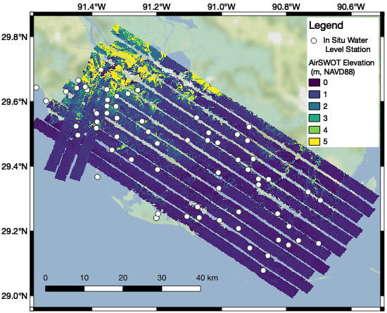
4.1. Water Surface Elevation

Validation of AirSWOT WSE estimates with all in situ water level measurements (Section 3.2) is presented in Figure 7 as a scatter plot including all three days of the AirSWOT campaign. The source of in situ data is identified with different colors.

We report the overall empirical uncertainty of the AirSWOT water levels in the form of mean absolute error (MAE) and root mean square error (RMSE) statistics. The MAE was calculated as follows:

$$\mathrm{MAE}=\mathbb{E}\left(\left|{\overrightarrow{h}}_{AirSWOT}-{\overrightarrow{h}}_{Station}\right|\right)$$

(10)

where $\mathbb{E}$ is the expectation operator (sample mean in this case), | | is the absolute value (applied to each element of the vector individually), ${\overrightarrow{h}}_{AirSWOT}$ is a vector of the estimated AirSWOT WSEs at each water level station, and ${\overrightarrow{h}}_{Station}$ is a vector of in situ water levels measured at each station (interpolated to the AirSWOT acquisition time using linear interpolation between the two closest measurements).

The RMSE was calculated as follows:

$$\mathrm{RMSE}=\sqrt{\mathbb{E}\left({\left({\overrightarrow{h}}_{AirSWOT}-{\overrightarrow{h}}_{Station}\right)}^2\right)}$$

(11)

where the exponent is applied to each element of the vector individually.

The MAE for all validation stations was 13 cm (RMSE of 17 cm), with the largest errors observed for some of the CRMS stations. The uncertainty calculated using only non-CRMS validation stations is 4 and 5 cm for MAE and RMSE, respectively. We determined the largest errors occur at higher AirSWOT incidence angles (Figure 8). Above incidence angles of about 15${}^{\circ }$, errors increase for the CRMS and calibration stations. The non-CRMS stations show smaller errors than the CRMS stations, and also appear to be less affected by incidence angle, though one calibration station at very far range does show a bias of 18 cm. One possible explanation for the correlation between elevation error and incidence angle is that the CRMS stations tend to be in areas with more vegetation, particularly emergent vegetation. Vegetation-related InSAR elevation biases are greater in magnitude at higher incidence angles [50,51]. CRMS stations also tend to be in areas with thinner river channels, which can make it more difficult to filter out areas contaminated by layover. Since there are fewer water pixels in the averaging window, any localized errors (such as layover) will tend to have a greater impact on the mean elevation of the pixels within the window, causing the MAD outlier filter to be less effective. In addition, errors in the AirSWOT phase calibration will result in larger elevation errors at far range than at near range, as $\frac{dh}{d\varphi }$ increases with incidence angle [14].

We found that limiting our analysis of CRMS stations to those located at AirSWOT incidence angles of less than 15${}^{\circ }$ significantly decreased the uncertainty as shown in Figure 9. The MAE decreased to 10 cm, with RMSE of 12 cm. This is only 1–2 cm larger than the uncertainty of the calibration stations. A linear fit applied to all station types has equation $y=0.99x+0.06$ with $r^2=0.89$, showing strong agreement between AirSWOT and in situ WSE. We did not restrict the incidence angle of the non-CRMS validation stations because these stations showed less of an elevation error vs. incidence angle trend, and the non-CRMS stations are more limited in number than the CRMS stations.

The WSE uncertainty observed in this study is within the range of those reported in previous studies using AirSWOT. In two previous studies of the Tanana River in Alaska, Altenau et al. [27,28] reported RMSE values of 9 cm and 11.8 cm. However, we note that we use a slightly smaller window size for our spatial averaging than in those studies. We use a 0.5 km${}^2$ window, while Altenau et al. use 1 km${}^2$ areas. Tuozzolo et al. [30] reported RMSE of 11.6 cm compared to in situ data over the Willamette River, Oregon, when using a 1 km shifting window to perform the averaging. Pitcher et al. [29] tested window sizes of both 1 km${}^2$ and 0.0625 km${}^2$ for a study in the Yukon Flats Basin in Alaska, and reported RMSE values of 8 and 15 cm, respectively, for rivers only. For lakes, Pitcher et al. reported RMSE of 21 cm.

Overall, our results show a high level of agreement between the AirSWOT WSE estimates and the in situ data. The similarity in the error levels of the calibration and validation stations suggest our calibration procedure is robust and not overfitted, as it produces accurate AirSWOT WSE estimates for both the calibration and validation water level data.

4.2. Measuring Water Level Change

We assess the consistency of AirSWOT WSE measurements over time by looking at the relative change in WSE between repeat AirSWOT acquisitions. The results are shown in Figure 10. Change in WSE was calculated for all in situ water level stations observed at least twice. As in Figure 9, we excluded CRMS stations observed at AirSWOT incidence angles ≥15${}^{\circ }$. The MAE of the WSE change estimates is slightly greater than the instantaneous WSE measurements—MAE of 11 cm and RMSE of 14 cm. The linear fit including all stations was found to be $y=1.05x-0.04$ with $r^2=0.95$, showing good agreement between AirSWOT and in situ.

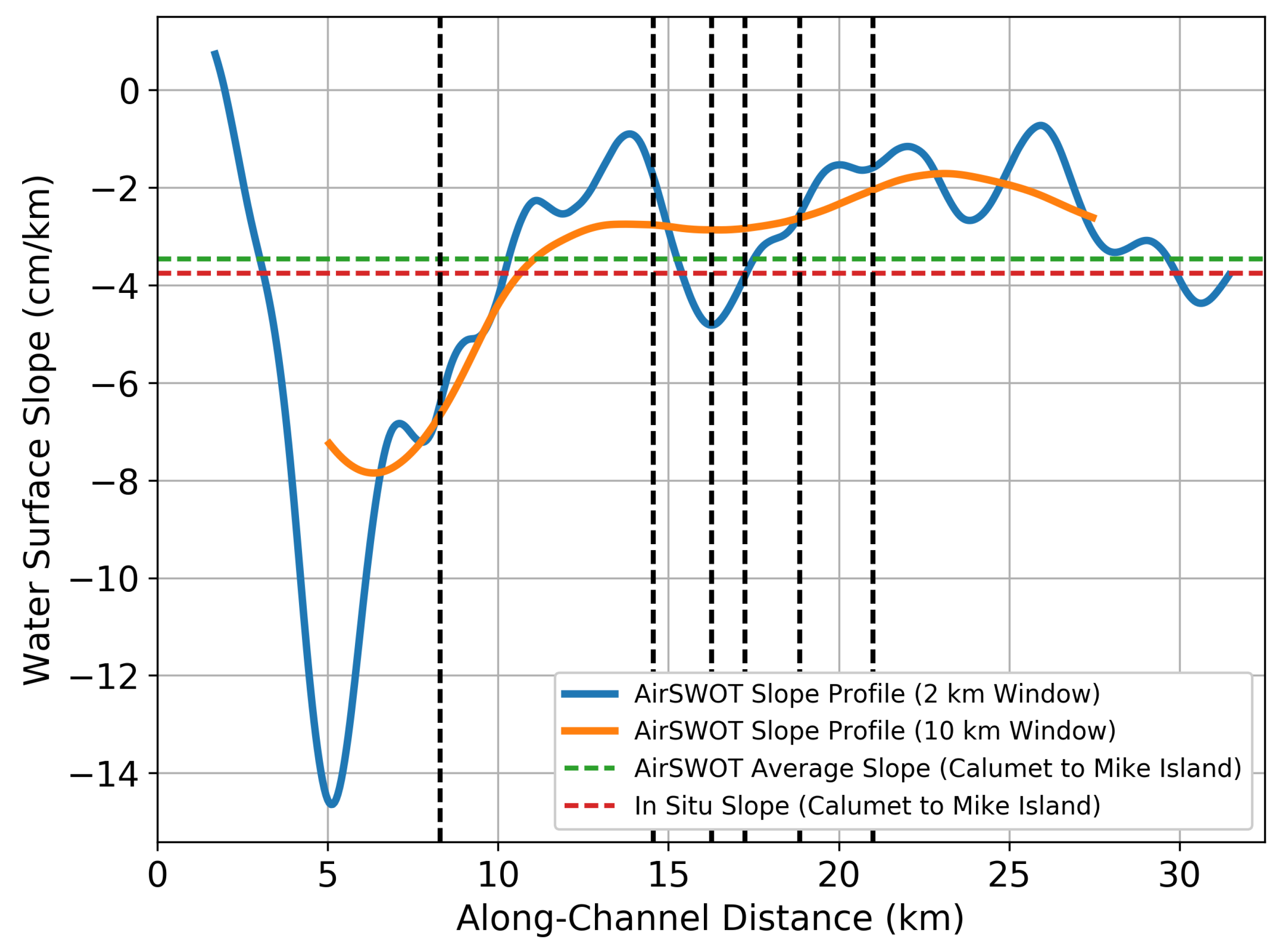
4.3. Water Surface Slope in the Wax Lake Outlet

AirSWOT can generate spatially continuous maps of WSE and WSS in a very short time period. Figure 11 shows a WSE river profile along the Wax Lake Outlet for an AirSWOT flight line acquired on 9 May 2015. The profile shows AirSWOT WSE as a function of distance along the channel, with the in situ water level data shown for comparison. We calculate the WSE profile by first creating a user-defined profile line along the Wax Lake Outlet, which is shown as the red line in Figure 11b. For each AirSWOT pixel in the area we reproject the data from the SCH coordinate system [54] to an along-channel and cross-channel coordinate system using the AirSWOT geolocation information and the manually drawn profile line. To remove AirSWOT pixels far away from the river channel, we discard pixels with cross-channel coordinates less than -700 m or greater than 900 m (distances from the profile line). While these bounds are wider than the Wax Lake Outlet itself, they were chosen to include a large portion of the river delta. The bounds are asymmetrical around zero because the manually drawn profile line isn’t located at the center of the river—it was drawn along the western riverbank of the Wax Lake Outlet.

To calculate the AirSWOT WSE along the profile, we performed a moving average, again removing outliers (as in Section 3.2), over a window length of 1 km in the along-channel direction, generating a WSE sample every 50 m along the profile. Again, water pixels were filtered using the land mask and 10 m buffer, followed by fixed thresholding and MAD filtering [55]. When taking the moving average, we also calculate the standard error of the AirSWOT pixels within the moving window and estimate the AirSWOT WSE uncertainty as described at the end of Section 3.2. The estimated AirSWOT WSE uncertainty is shown as the shaded blue region in the profile (±1$\sigma$ around the AirSWOT WSE estimate). After calculating the moving average, we perform further smoothing of the AirSWOT profile using a first order Savitzky-Golay filter with a window size of 2 km [56]. We use this additional smoothing to reduce the effects of noise and also to calculate profiles of WSS vs. along-channel distance (see below). We perform the moving average and Savitzky-Golay filter separately because the Savitzky-Golay filter must be applied to regularly sampled data, and because performing these steps in succession performs more smoothing than if the Savitzky-Golay filter was applied directly to the AirSWOT pixel elevations.

The dashed vertical black lines in the profile (Figure 11a) show the main confluence locations along the channel, which correspond to the dashes along the red line in the reference image below the profile (Figure 11b). The first confluence is the Intracoastal Waterway (ICW). Upstream of the ICW, the Wax Lake Outlet has a significantly steeper WSS than downstream of the ICW.

The profile shows the in situ water levels for the USGS Calumet, CRMS 0479, and LSU Mike Island stations. At the downstream end of the profile, the AirSWOT WSE is slightly overestimated compared to the station data, though still within the estimated AirSWOT WSE uncertainty.

On 8 May and 11 May, AirSWOT WSE profiles along the Wax Lake Outlet have only partial coverage due to low radar backscatter. This phenomenon has been observed in several campaigns and is generally referred to as “dark water”. It results from specular reflection of microwaves over a smooth water surface often encountered in very low wind conditions. The ${\sigma }^0$ of “dark water” is close to or below the AirSWOT instrument noise level, resulting in very low interferometric coherence, and thus noisy interferometric phase. Nonetheless, partial profiles were extracted for 8 May and 11 May (Figure 12) and suffice to estimate large scale WSS.

We note that in some of the areas where the profile could be estimated, erroneous WSE measurements (e.g., slopes in the wrong direction) are found at the edges of disconnected segments of the WSE profiles. A possible explanation is that while the water was specular, layover signals caused by vegetation along the river bank were interpreted as water surface signal. Another explanation is that when the amount of valid water data is small, the profile is more sensitive to errors in the water mask which allow land pixels to be incorrectly included in the profile. Despite the discontinuities in the WSE profile for two days of the campaign, we can use the AirSWOT measurements to calculate the overall WSS along the river channel between the USGS Calumet and LSU Mike Island stations.

A comparison of in situ vs. AirSWOT-derived WSS estimates for the Wax Lake Outlet are shown in

Table 3. Comparison of in situ and AirSWOT water surface slope estimates for the Wax Lake Outlet, between the USGS Calumet and NOAA Eugene Island stations.

Date	In Situ Slope	AirSWOT Slope	AirSWOT	Slope Error
	(cm/km)	(cm/km)	(cm/km)	(Percent)
8 May	−4.02	−4.06	−0.0414	−1.03
9 May	−3.75	−3.47	0.287	7.65
11 May	−4.50	−4.33	0.170	3.77

. To compute these slopes, we simply took the rise over run for the AirSWOT and in situ data at the Calumet and Mike Island stations. The largest error was for the 9 May flight, with absolute WSS error of 0.29 cm/km, corresponding to a percent error of 7.7%. The other two flights had smaller slope errors: −0.041 cm/km (−1.0%) on 8 May, and 0.17 cm/km (3.8%) on 11 May.

These WSS errors are significantly smaller than those reported in previous studies using AirSWOT to measure WSS [27,28,29,30], which generally found WSS errors on the order of 1.0 cm/km. However, we note that while those previous studies calculated WSS over 10 km reaches, here we calculate the slope between the USGS station at Calumet and the LSU Mike Island water level gauge, which are separated by almost 24 km. Unfortunately, we cannot accurately validate WSS over 10 km reaches of the Wax Lake Outlet due to the sparse coverage of the available in situ water level data in this location, as well as the void data caused by specular water on the 8 May and 11 May flights.

In general, we expect longer river reach distances to yield smaller WSS errors, as has been shown by Altenau et al. [28]. This is the case because as the river reach distance increases, the denominator of the slope equation (the reach distance) increases, but the error in the numerator of the slope equation (the change in water level along the reach) remains the same. Another explanation for these small WSS errors is that the Wax Lake Outlet is relatively straight, such that the AirSWOT incidence angle range was small between Calumet and Mike Island. This reduces the effect of any incidence angle-dependent errors, such as elevation biases due to residual errors in the phase calibration. The fact that our calibration procedure uses in situ data may also contribute to our better results.

One main advantage of AirSWOT or other remote sensing techniques compared to in situ data is the spatial continuity of the WSE and WSS estimates. In addition to deriving an average WSS between stations, AirSWOT can produce a profile of WSE and WSS along a river channel, in particular when there are no “dark water” issues. A WSS profile for the 9 May data is shown in Figure 13. The blue line shows WSS estimated using a first order Savitzky-Golay filter with a 2 km moving window, the same window size used to produce the WSE profiles. We also produced a WSS profile using a 10 km moving window, to match the 10 km reach length used in other AirSWOT studies [27,28,29,30]. The WSS profiles do not extend to the full length of the WSE profiles due to the length of the Savitzky-Golay filter.

AirSWOT-derived WSS of the Wax Lake Outlet was steepest near the USGS Calumet station, reaching a value of −14 cm/km before the slope decreased in magnitude as water approached the ICW (denoted by the first dashed black line). Downstream of the ICW, WSS mostly varied between −4 to −1 cm/km. It is not possible to validate these fine resolution WSS estimates without a dense set of in situ water level measurements. A future study should plan for a spatially dense set of in situ measurements over the primary river channels, similar to other studies [27,28,29,30].

5. Conclusions

We have investigated and demonstrated the use of AirSWOT to map WSE and WSS in coastal marsh environments. Our results show AirSWOT’s capabilities as a science instrument to support the upcoming Delta-X campaign and SWOT calibration/validation efforts. SWOT will provide a global perspective of WSE and WSS when it launches in 2022, while the airborne platform of AirSWOT enables focused studies at fine spatial and temporal resolution. This makes AirSWOT a particularly valuable instrument in highly dynamic and spatially complex coastal environments.

We implemented a data-driven method to calibrate the AirSWOT interferometric phase, which estimates and then removes time-varying differential phase delays between channels in the radar hardware. Our method uses non-vegetated water surfaces to remove instrument-related cross-track elevation slope and in situ water level measurements to remove remaining biases. Our method can be applied to future AirSWOT campaigns in coastal deltas and estuaries (e.g., the Delta-X campaign). While other AirSWOT studies [27,28,29,30] have focused on science results, this study introduces the details of AirSWOT phase calibration.

After applying the phase calibration method, we validated AirSWOT WSE in open water and found RMS errors of 12 cm over areas less than 0.5 km${}^2$. The SWOT science requirement for WSE accuracy is 10 cm RMSE averaged over a water area of 1 km${}^2$. While our RMSE is slightly larger, we averaged over a much smaller area to produce this error level. We only included results in our analysis if they were averaged over at least 1500 AirSWOT pixels, which covers a water area of only 0.0375 km${}^2$. Our error levels are similar to that reported in previous AirSWOT studies [27,28,29,30].

We used AirSWOT to estimate profiles of WSE and WSS along the Wax Lake Outlet river channel, with slope error of less than 0.3 cm/km on all three days of the campaign, less than 8% of in situ WSS. AirSWOT can estimate WSS with very high accuracy. The slope errors we reported are less than in previous studies [27,28,29,30], but we noted that the Wax Lake Outlet is a very straight river channel, reducing the potential effect of incidence angle-dependent errors (i.e., phase calibration errors).

This is the first study using AirSWOT to estimate WSE and WSS in coastal deltas and wetlands. Despite the challenges involved when processing AirSWOT data in these complex and spatially heterogeneous environments, our results demonstrate that AirSWOT provides accurate estimates of open water WSE and WSS in coastal deltas. The methods and results from this study will be used to support the future Delta-X and SWOT calibration campaigns.

References

1. Gleick, P.H. Water Use. Ann. Rev. Environ. Resour. 2003, 28, 275–314. [Google Scholar] [CrossRef]
2. Famiglietti, J.S.; Rodell, M. Water in the Balance. Science 2013, 340, 1300–1301. [Google Scholar] [CrossRef] [PubMed]
3. Hannah, D.M.; Demuth, S.; van Lanen, H.A.J.; Looser, U.; Prudhomme, C.; Rees, G.; Stahl, K.; Tallaksen, L.M. Large-scale river flow archives: Importance, current status and future needs. Hydrol. Process. 2011, 25, 1191–1200. [Google Scholar] [CrossRef]
4. Alsdorf, D.E.; Rodríguez, E.; Lettenmaier, D.P. Measuring surface water from space. Rev. Geophys. 2007, 45, 1–24. [Google Scholar] [CrossRef]
5. Durand, M.; Rodriguez, E.; Alsdorf, D.E.; Trigg, M. Estimating River Depth From Remote Sensing Swath Interferometry Measurements of River Height, Slope, and Width. IEEE J. Sel. Top. Appl. Earth Obs. Remote Sens. 2010, 3, 20–31. [Google Scholar] [CrossRef]
6. Smith, L.C.; Isacks, B.L.; Forster, R.R.; Bloom, A.L.; Preuss, I. Estimation of discharge from braided glacial rivers using ERS 1 synthetic aperture radar: First results. Water Resour. Res. 1995, 31, 1325–1329. [Google Scholar] [CrossRef]
7. Smith, L.C.; Isacks, B.L.; Bloom, A.L.; Murray, A.B. Estimation of Discharge From Three Braided Rivers Using Synthetic Aperture Radar Satellite Imagery: Potential Application to Ungaged Basins. Water Resour. Res. 1996, 32, 2021–2034. [Google Scholar] [CrossRef]
8. Alsdorf, D.E.; Smith, L.C.; Melack, J.M. Amazon floodplain water level changes measured with interferometric SIR-C radar. IEEE Trans. Geosci. Remote Sens. 2001, 39, 423–431. [Google Scholar] [CrossRef]
9. Lu, Z.; Kwoun, O. Radarsat-1 and ERS InSAR Analysis Over Southeastern Coastal Louisiana: Implications for Mapping Water-Level Changes Beneath Swamp Forests. IEEE Trans. Geosci. Remote Sens. 2008, 46, 2167–2184. [Google Scholar] [CrossRef]
10. Biancamaria, S.; Hossain, F.; Lettenmaier, D.P. Forecasting transboundary river water elevations from space. Geophys. Res. Lett. 2011, 38. [Google Scholar] [CrossRef]
11. Hong, S.; Wdowinski, S. Multitemporal Multitrack Monitoring of Wetland Water Levels in the Florida Everglades Using ALOS PALSAR Data With Interferometric Processing. IEEE Geosci. Remote Sens. Lett. 2014, 11, 1355–1359. [Google Scholar] [CrossRef]
12. Hossain, F.; Siddique-E-Akbor, A.H.; Mazumder, L.C.; ShahNewaz, S.M.; Biancamaria, S.; Lee, H.; Shum, C.K. Proof of Concept of an Altimeter-Based River Forecasting System for Transboundary Flow Inside Bangladesh. IEEE J. Sel. Top. App. Earth Obs. Remote Sens. 2014, 7, 587–601. [Google Scholar] [CrossRef]
13. Okeowo, M.A.; Lee, H.; Hossain, F.; Getirana, A. Automated Generation of Lakes and Reservoirs Water Elevation Changes From Satellite Radar Altimetry. IEEE J. Sel. Top. Appl. Earth Obs. Remote Sens. 2017, 10, 3465–3481. [Google Scholar] [CrossRef]
14. Rosen, P.A.; Hensley, S.; Joughin, I.R.; Li, F.K.; Madsen, S.N.; Rodriguez, E.; Goldstein, R.M. Synthetic aperture radar interferometry. Proc. IEEE 2000, 88, 333–382. [Google Scholar] [CrossRef]
15. Fu, L.L.; Alsdorf, D.; Rodriguez, E.; Morrow, R.; Mognard, N.; Lambin, J.; Vaze, P.; Lafon, T. The SWOT (Surface Water and Ocean Topography) mission: Spaceborne radar interferometry for oceanographic and hydrological applications. In Proceedings of the OCEANOBS’09 Conference, Venice, Italy, 21–25 September 2009. [Google Scholar]
16. Durand, M.; Fu, L.; Lettenmaier, D.P.; Alsdorf, D.E.; Rodriguez, E.; Esteban-Fernandez, D. The Surface Water and Ocean Topography Mission: Observing Terrestrial Surface Water and Oceanic Submesoscale Eddies. Proc. IEEE 2010, 98, 766–779. [Google Scholar] [CrossRef]
17. Neeck, S.P.; Lindstrom, E.J.; Vaze, P.V.; Fu, L.L. Surface Water and Ocean Topography (SWOT) mission. In Sensors, Systems, and Next-Generation Satellites XVI; International Society for Optics and Photonics: Bellingham, DC, USA, 2012; Volume 8533, p. 85330G. [Google Scholar]
18. Biancamaria, S.; Lettenmaier, D.P.; Pavelsky, T.M. The SWOT mission and its capabilities for land hydrology. In Remote Sensing and Water Resources; Springer: Cham, Switzerland, 2016; pp. 117–147. [Google Scholar]
19. Biancamaria, S.; Andreadis, K.M.; Durand, M.; Clark, E.A.; Rodriguez, E.; Mognard, N.M.; Alsdorf, D.E.; Lettenmaier, D.P.; Oudin, Y. Preliminary Characterization of SWOT Hydrology Error Budget and Global Capabilities. IEEE J. Sel. Top. Appl. Earth Obs. Remote Sens. 2010, 3, 6–19. [Google Scholar] [CrossRef]
20. Fjørtoft, R.; Gaudin, J.M.; Pourthie, N.; Lalaurie, J.C.; Mallet, A.; Nouvel, J.F.; Martinot-Lagarde, J.; Oriot, H.; Borderies, P.; Ruiz, C.; et al. KaRIn on SWOT: Characteristics of near-nadir Ka-band interferometric SAR imagery. IEEE Trans. Geosci. Remote Sens. 2013, 52, 2172–2185. [Google Scholar] [CrossRef]
21. Rodriguez, E. Surface Water and Ocean Topography Mission (SWOT): Science Requirements Document. SWOT NASA/JPL Project, Pasadena, Calif. Available online: https://swot.jpl.nasa.gov/files/swot/SRD_021215.pdf (accessed on 1 November 2019).
22. Pavelsky, T.M.; Durand, M.T.; Andreadis, K.M.; Beighley, R.E.; Paiva, R.C.; Allen, G.H.; Miller, Z.F. Assessing the potential global extent of SWOT river discharge observations. J. Hydrol. 2014, 519, 1516–1525. [Google Scholar] [CrossRef]
23. Moller, D.; Rodriguez, E.; Carswell, J.; Esteban-Fernandez, D. AirSWOT—A calibration/validation platform for the SWOT mission. In Proceedings of the International Geoscience and Remote Sensing Symposium, Vancouver, BC, Canada, 24–29 July 2011. [Google Scholar]
24. Moller, D.; Esteban-Fernandez, D. Near-Nadir Ka-band Field Observations of Freshwater Bodies. In Remote Sensing of the Terrestrial Water Cycle; American Geophysical Union (AGU): Washington, DC, USA, 2014; Chapter 9; pp. 143–155. [Google Scholar] [CrossRef]
25. Wu, X.; Hensley, S.; Rodriguez, E.; Moller, D.; Muellerschoen, R.; Michel, T. Near nadir Ka-band sar interferometry: SWOT airborne experiment. In Proceedings of the 2011 IEEE International Geoscience and Remote Sensing Symposium, Vancouver, BC, Canada, 24–29 July 2011; pp. 2681–2684. [Google Scholar] [CrossRef]
26. Moller, D.; Farquharson, G.; Esteban-Fernandez, D. Assessment of near-nadir correlation characteristics over water bodies using interferometric SAR: Implications for the SWOT mission. In Proceedings of the 2016 IEEE International Geoscience and Remote Sensing Symposium (IGARSS), Beijing, China, 10–15 July 2016; pp. 3219–3222. [Google Scholar] [CrossRef]
27. Altenau, E.H.; Pavelsky, T.M.; Moller, D.; Lion, C.; Pitcher, L.H.; Allen, G.H.; Bates, P.D.; Calmant, S.; Durand, M.; Smith, L.C. AirSWOT measurements of river water surface elevation and slope: Tanana River, AK. Geophys. Res. Lett. 2017, 44, 181–189. [Google Scholar] [CrossRef]
28. Altenau, E.H.; Pavelsky, T.M.; Moller, D.; Pitcher, L.H.; Bates, P.D.; Durand, M.T.; Smith, L.C. Temporal variations in river water surface elevation and slope captured by AirSWOT. Remote Sens. Environ. 2019, 224, 304–316. [Google Scholar] [CrossRef]
29. Pitcher, L.H.; Pavelsky, T.M.; Smith, L.C.; Moller, D.K.; Altenau, E.H.; Allen, G.H.; Lion, C.; Butman, D.; Cooley, S.W.; Fayne, J.V.; et al. AirSWOT InSAR mapping of surface water elevations and hydraulic gradients across the Yukon Flats Basin, Alaska. Water Resour. Res. 2019, 55, 937–953. [Google Scholar] [CrossRef]
30. Tuozzolo, S.; Lind, G.; Overstreet, B.; Mangano, J.; Fonstad, M.; Hagemann, M.; Frasson, R.P.M.; Larnier, K.; Garambois, P.A.; Monnier, J.; et al. Estimating River Discharge With Swath Altimetry: A Proof of Concept Using AirSWOT Observations. Geophys. Res. Lett. 2019, 46, 1459–1466. [Google Scholar] [CrossRef]
31. Fayne, J.V.; Smith, L.C.; Pitcher, L.H.; Kyzivat, E.D.; Cooley, S.W.; Cooper, M.G.; Denbina, M.; Chen, A.; Chen, C.; Pavelsky, T.M. First Airborne Observations of Arctic-Boreal Water Surface Elevations from AirSWOT Ka-Band InSAR and LVIS LiDAR. Environ. Res. Lett. 2019, 14, 080201. [Google Scholar]
32. Turki, I.; Laignel, B.; Chevalier, L.; Costa, S.; Massei, N. On the Investigation of the Sea-Level Variability in Coastal Zones Using SWOT Satellite Mission: Example of the Eastern English Channel (Western France). IEEE J. Sel. Top. Appl. Earth Obs. Remote Sens. 2015, 8, 1564–1569. [Google Scholar] [CrossRef]
33. Chevalier, L.; Desroches, D.; Laignel, B.; Fjørtoft, R.; Turki, I.; Allain, D.; Lyard, F.; Blumstein, D.; Salameh, E. High-Resolution SWOT Simulations of the Macrotidal Seine Estuary in Different Hydrodynamic Conditions. IEEE Geosci. Remote Sens. Lett. 2019, 16, 5–9. [Google Scholar] [CrossRef]
34. Mitra, S.; Wassmann, R.; Vlek, P.L. An appraisal of global wetland area and its organic carbon stock. Curr. Sci. 2005, 88, 25–35. [Google Scholar]
35. Mitsch, W.; Gosselink, J. Wetlands; Wiley: Hoboken, NJ, USA, 2007. [Google Scholar]
36. Milliman, J.D.; Meade, R.H. World-Wide Delivery of River Sediment to the Oceans. J. Geol. 1983, 91, 1–21. [Google Scholar] [CrossRef]
37. Kyzivat, E.D.; Smith, L.; Pitcher, L.; Fayne, J.; Cooley, S.; Cooper, M.; Topp, S.; Langhorst, T.; Harlan, M.; Horvat, C.; et al. A High-Resolution Airborne Color-Infrared Camera Water Mask for the NASA ABoVE Campaign. Remote Sens. 2019, 11, 2163. [Google Scholar] [CrossRef]
38. Thomas, N.; Simard, M.; Castañeda-Moya, E.; Byrd, K.; Windham-Myers, L.; Bevington, A.; Twilley, R.R. High-resolution mapping of biomass and distribution of marsh and forested wetlands in southeastern coastal Louisiana. Int. J. Appl. Earth Obs. Geoinf. 2019, 80, 257–267. [Google Scholar] [CrossRef]
39. Goldstein, R.M.; Zebker, H.A. Interferometric radar measurement of ocean surface currents. Nature 1987, 328, 707–709. [Google Scholar] [CrossRef]
40. Romeiser, R.; Breit, H.; Eineder, M.; Runge, H. Demonstration of current measurements from space by along-track SAR interferometry with SRTM data. In Proceedings of the IEEE International Geoscience and Remote Sensing Symposium, Toronto, ON, Canada, 24–28 June 2002; Volume 1, pp. 158–160. [Google Scholar] [CrossRef]
41. Steyer, G.D.; Sasser, C.E.; Visser, J.M.; Swenson, E.M.; Nyman, J.A.; Raynie, R.C. A Proposed Coast-Wide Reference Monitoring System for Evaluating Wetland Restoration Trajectories in Louisiana. Environ. Monit. Assess. 2003, 81, 107–117. [Google Scholar] [CrossRef] [PubMed]
42. Perrien, S.; Personal Correspondence with USGS Baton Rouge Field Office. Private Communication, 2019.
43. White, S.A. VDatum: Vertical Datum Transformation Tool; Presented to the Hydrographic Services Review Panel: 2013. Available online: https://vdatum.noaa.gov/download/presentations/vdatum_webinar_2013.pdf (accessed on 1 November 2019).
44. Raney, R.K.; Vachon, P.W. A phase preserving SAR processor. In Proceedings of the IGARSS ’89 and Canadian Symposium on Remote Sensing, 12th, Vancouver, BC, Canada, 10–14 July 1989; Volume 1, pp. 2588–2591. [Google Scholar]
45. Freeman, A. SAR calibration: An overview. IEEE Trans. Geosci. Remote Sens. 1992, 30, 1107–1121. [Google Scholar] [CrossRef]
46. Bickel, D.L.; Hensley, W.H. Interferometric SAR phase difference calibration: Methods and results. In Proceedings of the IGARSS ’94-1994 IEEE International Geoscience and Remote Sensing Symposium, Pasadena, CA, USA, 8–12 August 1994; Volume 4, pp. 2259–2262. [Google Scholar] [CrossRef] [Green Version]
47. Gatti, G.; Tebaldini, S.; Mariotti d’Alessandro, M.; Rocca, F. ALGAE: A Fast Algebraic Estimation of Interferogram Phase Offsets in Space-Varying Geometries. IEEE Trans. Geosci. Remote Sens. 2011, 49, 2343–2353. [Google Scholar] [CrossRef]
48. SWOT Project. SWOT Calibration/Validation Plan (Initial Release). Available online: https://swot.jpl.nasa.gov/docs/D-75724_SWOT_Cal_Val_Plan_Initial_20180129u.pdf (accessed on 1 November 2019).
49. Waite, W.P.; MacDonald, H.C. “Vegetation Penetration” with K-Band Imaging Radars. IEEE Trans. Geosci. Electron. 1971, 9, 147–155. [Google Scholar] [CrossRef]
50. Treuhaft, R.N.; Madsen, S.N.; Moghaddam, M.; van Zyl, J.J. Vegetation characteristics and underlying topography from interferometric radar. Radio Sci. 1996, 31, 1449–1485. [Google Scholar] [CrossRef]
51. Askne, J.; Dammert, P.; Ulander, L.; Smith, G. C-band repeat-pass interferometric SAR observations of the forest. IEEE Trans. Geosci. Remote Sens. 1997, 35, 25–35. [Google Scholar] [CrossRef]
52. Rufino, G.; Moccia, A.; Esposito, S. DEM generation by means of ERS tandem data. IEEE Trans. Geosci. Remote Sens. 1998, 36, 1905–1912. [Google Scholar] [CrossRef]
53. Hueso Gonzalez, J.; Bachmann, M.; Krieger, G.; Fiedler, H. Development of the TanDEM-X Calibration Concept: Analysis of Systematic Errors. IEEE Trans. Geosci. Remote Sens. 2010, 48, 716–726. [Google Scholar] [CrossRef] [Green Version]
54. Zebker, H.A.; Hensley, S.; Shanker, P.; Wortham, C. Geodetically Accurate InSAR Data Processor. IEEE Trans. Geosci. Remote Sens. 2010, 48, 4309–4321. [Google Scholar] [CrossRef]
55. Leys, C.; Ley, C.; Klein, O.; Bernard, P.; Licata, L. Detecting outliers: Do not use standard deviation around the mean, use absolute deviation around the median. J. Exp. Soc. Psychol. 2013, 49, 764–766. [Google Scholar] [CrossRef] [Green Version]
56. Savitzky, A.; Golay, M.J.E. Smoothing and Differentiation of Data by Simplified Least Squares Procedures. Anal. Chem. 1964, 36, 1627–1639. [Google Scholar] [CrossRef]
Figure 1. Overview map showing the locations of in situ water level stations overlaid on the AirSWOT elevation maps for 9 May 2015. The two stations used as GCPs in the AirSWOT calibration procedure are annotated with text labels. The background image is by Stamen Design, using OpenStreetMap data (see Acknowledgements).
Remotesensing 11 02739 g001
Figure 2. Map of the Wax Lake and Atchafalaya Deltas, showing the in situ water level station locations overlaid on the AirSWOT elevations for 9 May 2015. Some of the stations used for validation are annotated with text labels, for reference. The locations of the two NOAA stations were adjusted because their original positions were outside of the AirSWOT data extents. The background image is by Stamen Design, using OpenStreetMap data (see Acknowledgements).
Remotesensing 11 02739 g002
Figure 3. Comparison of AirSWOT elevation before and after applying our calibration method. Figure 3a shows maps of AirSWOT elevations using the original phase drift parameters (left map) and after applying our calibration method (right map). Figure 3b shows AirSWOT elevation vs. incidence angle for the water polygons (red boxes) in Figure 3a. The solid lines show the mean AirSWOT elevation at each incidence angle, while the shaded region shows ± 1 σ around the mean. After our calibration procedure, the anomalous cross-track slope seen in the original results has been corrected.
Remotesensing 11 02739 g003
Figure 4. The areas that were excluded from the cross-track slope removal objective of the calibration procedure are shown in black. In the remaining non-masked areas, the calibration attempts to minimize the cross-track elevation slope with respect to the NAVD88 geoid.
Remotesensing 11 02739 g004
Figure 5. Phase drifts estimated by our calibration procedure for each day of the AirSWOT campaign. Early in each flight the estimated phase bias changes rapidly, but becomes more stable over time.
Remotesensing 11 02739 g005
Figure 6. Example of how the AirSWOT data is filtered to estimate WSE. Figure 6a shows the averaging window before (left) and after (right) filtering. The left image shows the AirSWOT elevation of each pixel within the square averaging window for the Calumet station using an AirSWOT flight line on 9 May 2015. The right image shows the pixels removed by the filter in various colors as listed in the legend. The black circle at the center of each image shows the location of the USGS Calumet station. Figure 6b shows the AirSWOT elevation distribution before filtering (top), after the land and land buffer filtering (middle), and after all filtering has been performed (bottom). The dashed lines show the mean elevation of each distribution, which get closer to the in situ water level (shown as the dashed black line) as each filtering step is performed.
Remotesensing 11 02739 g006
Figure 7. AirSWOT vs. in situ water level. The points are colored according to the type of water level station as shown in the legend. The dashed black line is y = x . The dashed red line is a linear fit applied to all station types, with equation and r 2 as shown on the plot.
Remotesensing 11 02739 g007
Figure 8. AirSWOT water level error vs. AirSWOT incidence angle. The error is shown as AirSWOT WSE minus in situ WSE. The points are colored according to the type of water level station as shown in the legend.
Remotesensing 11 02739 g008
Figure 9. AirSWOT vs. in situ water level, excluding CRMS stations at AirSWOT incidence angles ≥ 15 . The points are colored according to the type of water level station as shown in the legend. The dashed black line is y = x . The dashed red line is a linear fit applied to all station types, with equation and r 2 as shown on the plot.
Remotesensing 11 02739 g009
Figure 10. AirSWOT vs. in situ relative water level change, excluding CRMS stations at AirSWOT incidence angles of ≥15 . The points are colored according to the type of water level station as shown in the legend. The dashed black line is y = x . The dashed red line is a linear fit applied to all station types, with equation and r 2 as shown on the plot.
Remotesensing 11 02739 g010
Figure 11. AirSWOT WSE profile for 9 May (a) and a reference image showing the center line used to create the profile (b). In the reference image, the land mask (in black) is superimposed on the AirSWOT elevation map for 9 May. The Wax Lake Outlet center line used to generate the profile is shown in red. The dashes along the center line correspond to the vertical dashed black lines in the profile, and represent major inflow and outflow locations along the channel. In the profile, the solid blue line shows the estimated AirSWOT WSE along the profile, while the blue shaded region shows the estimated AirSWOT WSE uncertainty ( ± 1 σ ). The circular markers denote in situ water levels from the station data.
Remotesensing 11 02739 g011
Figure 12. AirSWOT WSE profiles for 8 May (Figure 12a) and 11 May (Figure 12b) showing the effects of “dark water” on AirSWOT WSE. “Dark water” results in void data and potential anomalies in the small, disconnected regions between the void data.
Remotesensing 11 02739 g012
Figure 13. AirSWOT WSS profile for 9 May. The vertical dashed black lines represent major inflow and outflow locations along the channel. The solid blue and orange lines show the estimated AirSWOT WSS using different window sizes, while the dashed horizontal lines show the average slope between the Calumet and Mike Island stations as estimated by AirSWOT and the in situ data.
Remotesensing 11 02739 g013