Differentially Deep Subspace Representation for Unsupervised Change Detection of SAR Images

Abstract

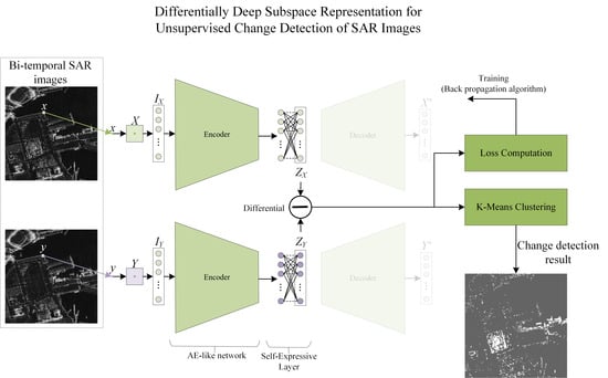
Temporal analysis of synthetic aperture radar (SAR) time series is a basic and significant issue in the remote sensing field. Change detection as well as other interpretation tasks of SAR images always involves non-linear/non-convex problems. Complex (non-linear) change criteria or models have thus been proposed for SAR images, instead of direct difference (e.g., change vector analysis) with/without linear transform (e.g., Principal Component Analysis, Slow Feature Analysis) used in optical image change detection. In this paper, inspired by the powerful deep learning techniques, we present a deep autoencoder (AE) based non-linear subspace representation for unsupervised change detection with multi-temporal SAR images. The proposed architecture is built upon an autoencoder-like (AE-like) network, which non-linearly maps the input SAR data into a latent space. Unlike normal AE networks, a self-expressive layer performing like principal component analysis (PCA) is added between the encoder and the decoder, which further transforms the mapped SAR data to mutually orthogonal subspaces. To make the proposed architecture more efficient at change detection tasks, the parameters are trained to minimize the representation difference of unchanged pixels in the deep subspace. Thus, the proposed architecture is namely the Differentially Deep Subspace Representation (DDSR) network for multi-temporal SAR images change detection. Experimental results on real datasets validate the effectiveness and superiority of the proposed architecture.

1. Introduction

Change detection with remote sensing images is the process of identifying and locating differences in regions of interest by observing them at different dates [1]. It is of great significance for many applications of remote sensing images, such as rapid mapping of disaster, land-use and land-cover monitoring and so on. Wessels et al. [2] use optical images with the reweighted multivariate alteration detection method to identify change areas, and then update the land-cover mapping. A multi-sensor change detection method between optical and synthetic aperture radar (SAR) imagery is proposed in [3] for earthquake damage assessment of buildings. Taubenbock et al. [4] propose a post-classification based change detection using optical and SAR data for urbanization monitoring. Multi-temporal airborne laser data is used to monitor forest change in [5]. In this paper, we tackle the issue of change detection using SAR images. Unlike optical remote sensing images, SAR images can be acquired under any weather condition at day or night; however, there usually are more challenges (i.e., non-linear/non-convex problems) for SAR image visual and machine interpretation due to the coherent imaging mechanism (speckle).

For change detection using remotely sensed optical images, the most widely used criterion is difference operator [1] (for single channel images) or change vector analysis [6,7,8] (for multi-band/spectral images). Due to the temporal spectral variance caused by different atmospheric conditions, illumination and sensor calibration, image transformation has been widely used to yield robust change detection criteria. The core idea of the image transformation is to transform the multi-band/spectral image into a specific feature space, in which the unchanged temporal pixel pairs have similar representations while the changed ones differ from each other. Principal component analysis (PCA) [9,10,11] is one of the state-of-the-art operators for modeling temporal spectral difference of unchanged pixels. Beyond PCA, Kauth-Thomas transformation [12], Gram-Schmidt orthonormalization process [13,14], multivariate alteration detection [15,16] and slow feature analysis [17,18] theories have been used for optical image change detection. However, these algorithms are mainly designed for optical images and usually fail to deal with SAR images with speckle.

Given SAR images, we may meet a more complex situation in which the multi-temporal images are in different feature spaces and changed/unchanged pixels are linearly non-sparable, due to the coherent imaging mechanism. Two main approaches have been developed in the literature: coherence change detection and incoherent change detection. The former uses the phase information of SAR time series to study the coherence map, which has strict limitations for the input multi-temporal SAR images [19]. The incoherent change detection more relies on the amplitude or intensity values of SAR data, for instance, the amplitude ratio or log-ratio [20]. Improvements have been proposed thanks to automatic thresholding methods [21] and multi-scale analysis to preserve details [22]. Lombardo and Oliver [23] propose a generalized likelihood ratio test given by the ratio between geometric and arithmetic means for SAR images. Quin et al. [24] extend the SAR ratio to more general cases with an adaptive and nonlinear threshold, which can be applied to not only SAR image pairs but also long-term SAR time series. Beyond change detection, Su et al. [25] propose a generalized likelihood ratio test based spectral cluster for temporal behaviours analysis of long-term SAR time series. Obviously, non-linear change criteria have been widely used for SAR images in the literature. However, these change criteria usually have noisy results due to the SAR speckle, or face a trade off between spatial resolution and smoothness of detecting results.

Recently, deep learning techniques have been experiencing a rapid growth and have achieved remarkable success in various fields. Given change detection issue using remotely sensed data, a large number of deep network architectures have been proposed. Improved UNet++ [26] is proposed to solve the error accumulation problems in the deep feature based change detection. Ji et al. [27] apply a Mask R-CNN based building change detection network with self-training ability, which does not need high-quality training samples. Dual learning-based Siamese framework in [28] can reduce the domain differences of bi-temporal images by retaining the intrinsic information and translating them into each other’s domain. A set of convolutional neural network features [29] have been used to compute the difference indices. Similarly, a spare autoencoder is applied in [30] to extract robust SAR features for change detection.

In this paper, we propose a differentially deep subspace representation (DDSR) for multi-temporal SAR images. The proposed network consists of a non-linear mapping network followed by a linear transform layer to deal with the complex patterns of changed and unchanged pixels in SAR images. The non-linear mapping network is built upon an autoencoder-like (AE-like) deep neural network, which can non-linearly map the noisy SAR data to a low-dimensional latent space. Contrary to normal autoencoder (AE) network, the proposed architecture is trained to minimize the representation difference of unchanged pixel pairs, instead of reconstruction error of the decoder. To better separate the unchanged and changed pixels in the latent space, a single-layer self-expressive network linearly transform the mapped SAR data into a mutually orthogonal subspace. In the transformed subspace, the unchanged pixel pairs have similar representation, while the temporally changed ones are comparatively different from each other. Changed pixels are finally identified by an unsupervised K-Means clustering method [31]. Note that a similar idea has been proposed in [32], in which the slow feature analysis [18] is applied to perform the linear transform, instead of our self-expressive network with the back propagation algorithm.

This paper is organized as follows. Section 2 briefly recalls the non-linear/linear subspace approaches. The proposed network is presented in Section 3, which is followed by the evaluation (Section 4) and the conclusion (Section 5).

2. Related Work

To deal with the nonlinearities in SAR change detection task, the proposed DDSR maps the bi-temporal SAR data into a subspace using a non-linear AE-like network followed by a linear self-expressive layer. The change criterion is computed by the DDSR difference of the input bi-temporal SAR images. Similar ideas have been proposed in the literature.

2.1. Deep Subspace Clustering

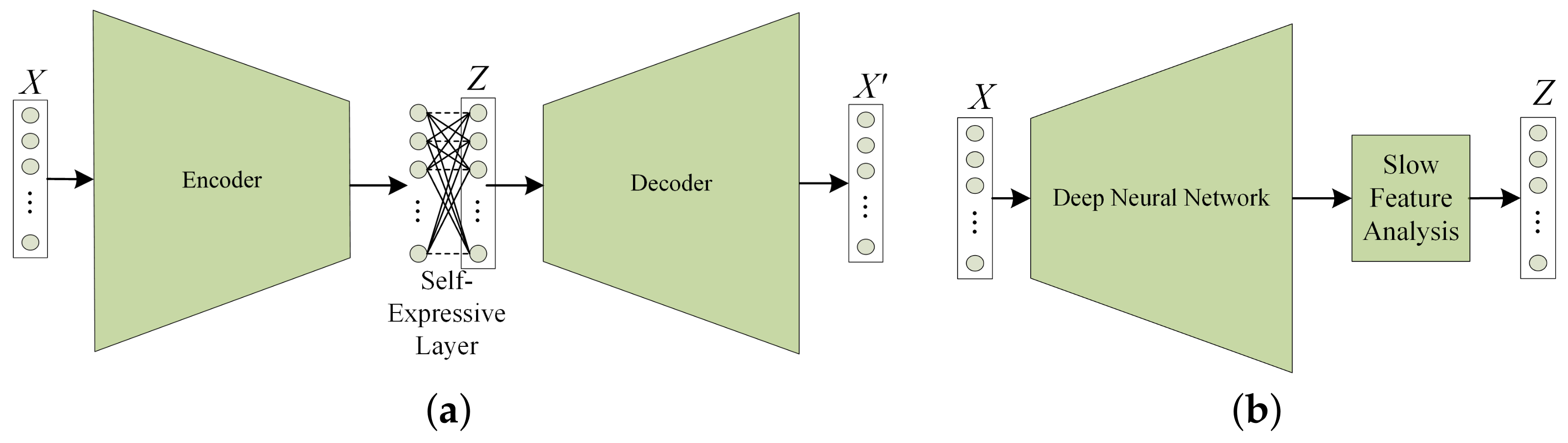
Ji et al. [33] propose a deep autoencoder framework for subspace clustering, in which a self-expressive layer has been introduced between the encoder and the decoder to learn the pairwise affinities of the input data through a standard backpropagation procedure. Figure 1a gives a brief illustration of this deep subspace clustering network. It provides an explicit non-linear mapping for the complex input data that is well-adapted to the subspace clustering, which yields significant improvement over the state-of-the-art subspace clustering solutions. A structured autoencoder in [34] introduces a global structure prior into the non-linear mapping.

These deep subspace approaches mainly focus on the clustering or recognition problems, in which the network weights are well trained to exploit the similar information among the input data, instead of the differential information used for change detection task. Even though these approaches can be easily adapted to change detection task, the performance might not be optimal. In this paper, the proposed architecture discards the decoder network and redesigns the network loss to adapt the SAR image change detection.

2.2. Deep Slow Feature Analysis Network

In [32], Du et al. present a slow feature analysis (SFA) theory based deep neural network for optical remote sensing change detection. This network non-linearly maps the input bi-temporal data into a higher dimensional space, as shown in Figure 1b. The classic slow feature analysis (SFA) algorithm is then applied to suppress the unchanged components and highlight the changed components of the mapped data. In our work, the non-linear mapping is our DDSR network, which performs a sparse autoencoder, which compacts the input data to lower dimensional space. In addition, compared with the SFA based linear transformation, the self-expressive layer can be trained to adapt well to the given task and the given dataset by the backpropagation algorithm.

3. Differentially Deep Subspace Representation (DDSR) for Change Detection

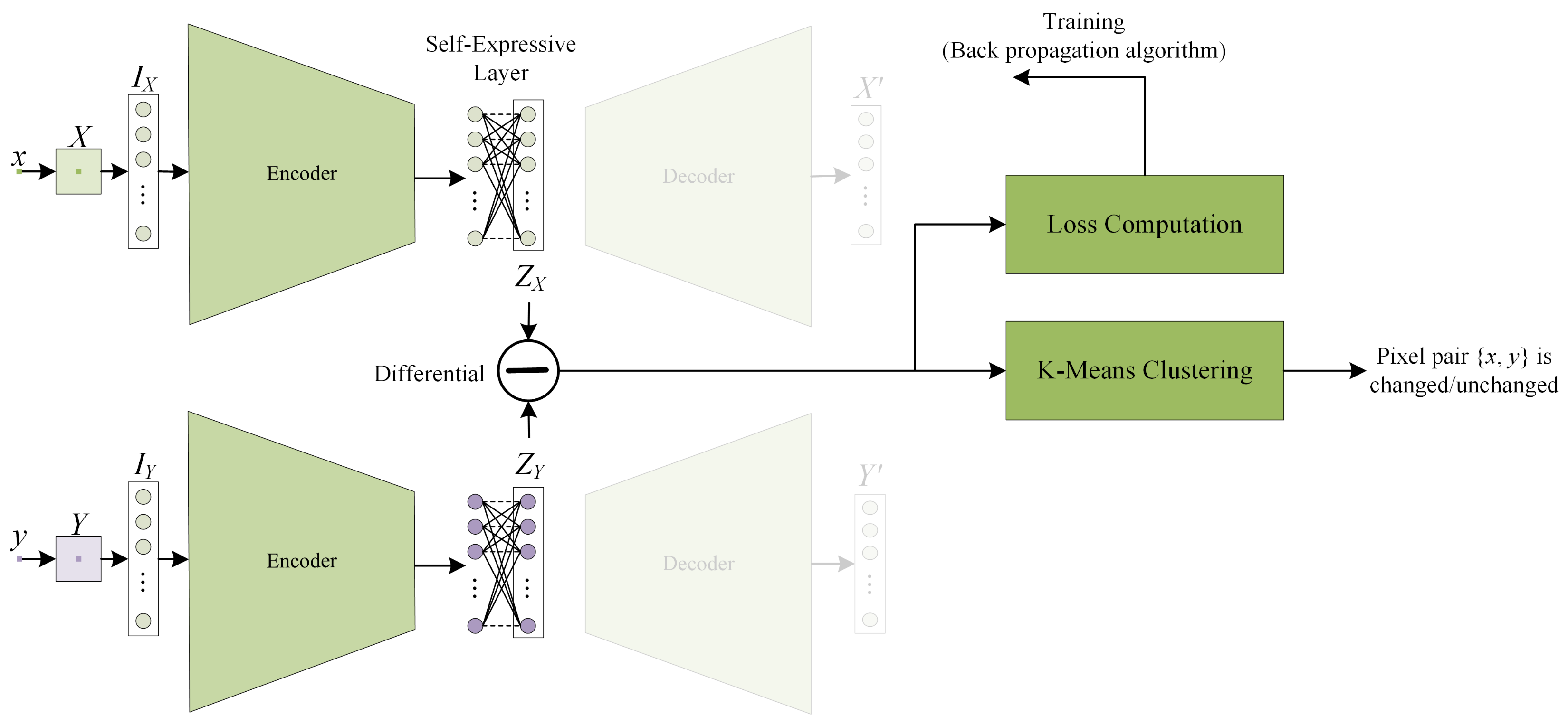
As far as we are concerned, the non-linear transformation for change detection generally outperforms linear ones, which can handle the complex patterns of the input data. Non-linear kernel based methods have also been proposed [35,36,37]; however, it is not clear whether the pre-defined kernels are suitable for SAR image change detection tasks. In this work, our goal is to learn an explicit mapping that makes the changed and unchangded pixel pairs more separable in the transformed subspaces. This section builds our architecture namely differentially deep subspace representation (DDSR) based on the classic autoencoder network. As shown in Figure 2, the non-linear part (the AE-like network) first maps the input bi-temporal SAR data into a low-dimensional latent space. The linear part (the self-expressive layer) further transforms the mapped SAR data to a subspace. Contrary to minimization of the reconstruction error, the proposed architecture is trained to compact unchanged pixel pairs and explode the changed ones in the subspace.

3.1. AE-Like Network Based Non-Linear Mapping

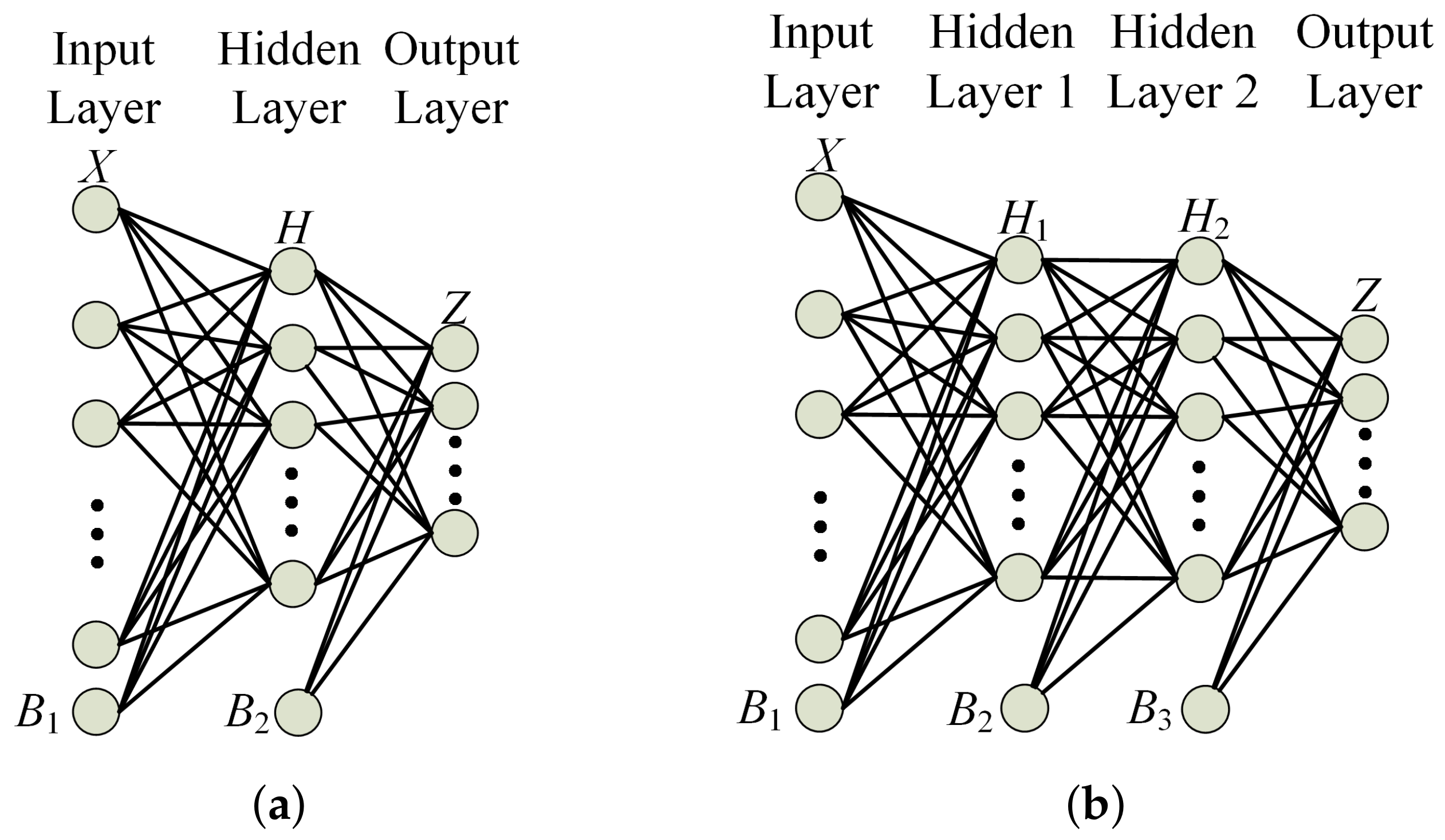
Basically, the encoder of the AE network is a classical multi-layer deep neural network. Each layer consisting of an input layer, a hidden layer and a output layer can non-linearly transform the input data to latent features. Given a pair of pixels $\{x,y\}\in \{{\mathbb{R}}^1,{\mathbb{R}}^1\}$, $\mathbf{X}\in {\mathbb{R}}^{\sqrt{N}\times \sqrt{N}}$ and $\mathbf{Y}\in {\mathbb{R}}^{\sqrt{N}\times \sqrt{N}}$ are corresponding patches with pixel x and y as center, respectively. In the proposed AE-like network, $\mathbf{I}\in {\mathbb{R}}^{N\times 1}$, $\mathbf{H}\in {\mathbb{R}}^{M\times 1}$ and $\mathbf{Z}\in {\mathbb{R}}^{M\times 1}$ ($N>M$) denote the input, hidden and output layer of the neural networks. At the first stage, the patch pair $\{\mathbf{X},\mathbf{Y}\}$ corresponding to pixel pair $\{x,y\}$ are reshaped to form input vector $\mathbf{I}$ (i.e., ${\mathbf{I}}_{\mathbf{X}}$ and ${\mathbf{I}}_{\mathbf{Y}}$). The hidden layer can be computed by

$$\mathbf{H}=f({\mathbf{W}}_{\mathbf{H}}\mathbf{I}+{\mathbf{B}}_{\mathbf{H}}),$$

(1)

where ${\mathbf{W}}_{\mathbf{H}}\in {\mathbb{R}}^{M\times N}$ denotes the weight matrix of the hidden layer, ${\mathbf{B}}_{\mathbf{H}}\in {\mathbb{R}}^M$ denotes the bias and f denotes the activation function performing the non-linear mapping. At the second stage, the latent feature $\mathbf{H}$ is mapped to the output by

$$\mathbf{Z}=g({\mathbf{W}}_{\mathbf{O}}\mathbf{H}+{\mathbf{B}}_{\mathbf{O}}).$$

(2)

where ${\mathbf{W}}_{\mathbf{O}}\in {\mathbb{R}}^{M\times M}$ denotes the weight matrix of the output layer, ${\mathbf{B}}_{\mathbf{O}}\in {\mathbb{R}}^M$ is the bias and g denotes the activation function. Finally, the weights ${\mathbf{W}}_{\mathrm{AE}}=\{{\mathbf{W}}_{\mathbf{H}},{\mathbf{B}}_{\mathbf{H}},{\mathbf{W}}_{\mathbf{O}},{\mathbf{B}}_{\mathbf{O}}\}$ of the AE-like network are learned by minimizing the target loss with the backpropagation algorithm. The so-called representation of the input data is the hidden layer. Generally, as the number of layers increases, the learning features are more abstract and more robust. The encoder with a different number of hidden layers are shown in Figure 3.

The classic AE networks are designed to extract efficient representation of the input data; thus, the reconstruction error of the decoder is one of the key minimization targets. However, in our work, the AE network trained by minimizing the reconstruction error may lose the efficiency of the change detection purpose, since the key information for the reconstruction might not be useful for the change detection tasks. Consequently, our DDSR architecture only keeps the encoder part that can non-linearly map the input bi-temporal SAR data to the low-dimensional space, and discards the decoder part including the reconstruction error in the loss.

3.2. Self-Expressive Layer Based Linear Transformation

As shown in Figure 2, the main motivation of the self-expressive layer is based on the PCA and SFA theories. However, unlike PCA or SFA, the linear transformation of our DDSR is learned by the backpropagation algorithm, instead of the classic or generalized eigenvalue decomposition. The data-driven strategy can make the self-expressive aspects more adaptive to the given datasets than PCA and SFA. Let $\mathbf{Z}\in {\mathbb{R}}^{M\times 1}$ and ${\mathbf{Z}}^{\prime }\in {\mathbb{R}}^{M\times 1}$ denote the input (i.e., the output of the AE-like network) and the output of the self-expressive layer.

$${\mathbf{Z}}^{\prime }={\mathbf{W}}_{\mathrm{SE}}\mathbf{Z},\mathrm{s}.\mathrm{t}.\mathrm{diag}\left({\mathbf{W}}_{\mathrm{SE}}\right)=0$$

(3)

where ${\mathbf{W}}_{\mathrm{SE}}\in {\mathbb{R}}^{M\times M}$ denotes the weights of the self-expressive layer. To form a mutually orthogonal subspace, each row vector in ${\mathbf{W}}_{\mathrm{SE}}$ has to be orthogonal to any other row vector in ${\mathbf{W}}_{\mathrm{SE}}$.

3.3. Network Architecture of DDSR

Since the pixel-wise change detection is strongly affected by the speckle, patch-wise strategy has been applied in this paper, i.e., a square image patch formed by a pixel and its surrounding pixels. Each patch pair $\{{\mathbf{I}}_{\mathbf{X}},{\mathbf{I}}_{\mathbf{Y}}\}$ with center pixel $\{x,y\}$ is reshaped to vector $\mathbf{X}\in {\mathbb{R}}^{N\times 1}$ and $\mathbf{Y}\in {\mathbb{R}}^{N\times 1}$ ($N=5\times 5$ in this paper), as shown in Figure 2. Through the AE-like network (Section 3.1), the input bi-temporal SAR patches $\mathbf{X}$ and $\mathbf{Y}$ are non-linearly mapped to a lower dimensional latent space, denoted by ${\mathbf{Z}}_{\mathbf{X}}\in {\mathbb{R}}^{M\times 1}$ and ${\mathbf{Z}}_{\mathbf{Y}}\in {\mathbb{R}}^{M\times 1}$ (where $N>M$). ${\mathbf{Z}}_{\mathbf{X}}$ and ${\mathbf{Z}}_{\mathbf{Y}}$ are then linearly transformed to ${\mathbf{Z}}_{\mathbf{X}}^{\prime }$ and ${\mathbf{Z}}_{\mathbf{Y}}^{\prime }$ by the self-expressive layer. The change criterion $\mathbf{r}$ between pixel x and y can be calculated by

$$\mathbf{r}=\parallel {\mathbf{Z}}_{\mathbf{X}}^{\prime }-{\mathbf{Z}}_{\mathbf{Y}}^{\prime }\parallel .$$

(4)

To identify the changed pixels, an unsupervised K-Means cluster is applied to classify $\left\{\mathbf{r}\right\}$ into the changed and unchanged groups.

3.4. Training Strategy

As shown in Figure 2, the classic AE network is adapted to handle the change detection task. The whole network is trained by minimizing the loss computed from the differential representation of the bi-temporal SAR patches.

$$\begin{array}{c}\hfill \{{\mathbf{W}}_{\mathrm{AE}},{\mathbf{W}}_{\mathrm{SE}}\}=\underset{{\mathbf{W}}_{\mathrm{AE}},{\mathbf{W}}_{\mathrm{SE}}}{\min }\mathrm{Loss}(\mathbf{\Lambda },{\mathbf{W}}_{\mathrm{AE}},{\mathbf{W}}_{\mathrm{SE}},{\mathbf{Z}}_{\mathbf{X}}^{\prime },{\mathbf{Z}}_{\mathbf{Y}}^{\prime }),\end{array}$$

(5)

where the loss can be calculated by

$$\begin{array}{cc}\hfill \mathrm{Loss}(\mathbf{\Lambda },{\mathbf{W}}_{\mathrm{AE}},{\mathbf{W}}_{\mathrm{SE}},{\mathbf{Z}}_{\mathbf{X}}^{\prime },{\mathbf{Z}}_{\mathbf{Y}}^{\prime })& =\parallel {\mathbf{Z}}_X^{\prime }-{\mathbf{Z}}_Y^{\prime }{\parallel }_2^2+{\lambda }_1\mathrm{Norm}\left({\mathbf{Z}}_X^{\prime },{\mathbf{Z}}_Y^{\prime }\right)+{\lambda }_2\mathrm{Regl}\left({\mathbf{W}}_{\mathrm{AE}},{\mathbf{W}}_{\mathrm{SE}}\right).\hfill \end{array}$$

(6)

$\parallel {\mathbf{Z}}_X^{\prime }-{\mathbf{Z}}_Y^{\prime }{\parallel }_2^2$ denotes the representation differential, $\mathrm{Norm}\left({\mathbf{Z}}_X^{\prime },{\mathbf{Z}}_Y^{\prime }\right)$ is the data constraint term and $\mathrm{Regl}\left({\mathbf{W}}_{\mathrm{AE}},{\mathbf{W}}_{\mathrm{SE}}\right)$ is the weight regularization term. The weights $\mathbf{\Lambda }=\{{\lambda }_1,{\lambda }_2\}$ control the balance terms in the loss function. The data constraint term ensures that the output of DDSR has significant information (avoiding a meaningless solution, i.e., ${\mathbf{W}}_{\mathrm{AE}}=0,{\mathbf{W}}_{\mathrm{SE}}=0$).

$$\begin{array}{c}\hfill \mathrm{Norm}\left({\mathbf{Z}}_X^{\prime },{\mathbf{Z}}_Y^{\prime }\right)={\left|\left|\mathrm{Var}\left({\mathbf{Z}}_X^{\prime }\right)-\mathbf{E}\right|\right|}_2^2+{\left|\left|\mathrm{Var}\left({\mathbf{Z}}_Y^{\prime }\right)-\mathbf{E}\right|\right|}_2^2\end{array}$$

(7)

where $\mathbf{E}\in {\mathbb{R}}^{M\times 1}$ denotes the is a column vector whose elements are all 1. Note that theoretically the non-zero variance constraint is enough. However, for the sake of simplification, the unite-variance constraint is used in the paper. The weight regularization term is calculated by

$$\begin{array}{c}\hfill \mathrm{Regl}\left({\mathbf{W}}_{\mathrm{AE}},{\mathbf{W}}_{\mathrm{SE}}\right)={\left|\left|{\mathbf{W}}_{\mathrm{AE}}\right|\right|}_2^2+{\left|\left|{\mathbf{W}}_{\mathrm{SE}}\right|\right|}_2^2+\sum \mathrm{Cor}({\mathbf{w}}_{\mathrm{SE}}^i,{\mathbf{w}}_{\mathrm{SE}}^j),\mathrm{s}.\mathrm{t}.i\ne j\end{array}$$

(8)

where ${\left|\left|{\mathbf{W}}_{\mathrm{AE}}\right|\right|}_2^2$ and ${\left|\left|{\mathbf{W}}_{\mathrm{SE}}\right|\right|}_2^2$ are classic regularization term. The third term controls the orthogonality of ${\mathbf{W}}_{\mathrm{SE}}$, in which $\mathrm{Cov}({\mathbf{w}}_{\mathrm{SE}}^i,{\mathbf{w}}_{\mathrm{SE}}^j)$ is the correlation coefficient between the i-th row vector and the j-th row vector of ${\mathbf{W}}_{\mathrm{SE}}$. Theoretically, the self-expressive layer performs like a PCA or SFA approach, for which the orthogonality is needed to have a complete and non-redundant representation. Without this orthogonality term, the output of DDSR will be a vector of a constant number.

3.5. Implementation Details

Since no labeled data is needed in the training stage, our DDSR is unsupervised. However, DDSR makes an assumption that the unchanged pixel pairs are much more than changed ones, since theoretically only unchanged pixel pairs meet the minimization of the proposed loss (Equation (6)). A similar assumption has also been used in slow feature analysis (SFA) based unsupervised change detection approach in [18]. In addition, this assumption might not hold when the given bi-temporal SAR images have a very long time interval (changed pixels/regions are more than unchanged ones). However, one can easily discard this assumption by introducing a pre-detection strategy (e.g., the classic log-ratio change detection approach) providing some unchanged pixel pairs as training samples. A similar strategy has been used in [30].

Since the proposed network focuses on the change detection task instead of the representation of the classic AE network, the network parameters are firstly initialized randomly, not by a pre-trained AE network. In the training stage, all the patch pairs are fed into the DDSR network. The Adam optimization algorithm is applied to minimize the loss (Equation (6)) and obtain the optimal parameters ${\mathbf{W}}_{\mathrm{AE}}$ and ${\mathbf{W}}_{\mathrm{SE}}$ with 0.1 learning rate. The number of iterations is 1500. In the testing stage, the change criterion $\mathbf{r}$ (Equation (4)) is computed pixel by pixel. The classic K-Means clustering method is then performed on $\left\{\mathbf{r}\right\}$ to group pixel pairs into two groups, in which the group with lower magnitude of cluster center $|\overline{\mathbf{r}}|$ is the unchanged group.

4. Experiment

In this section, we investigate the effectiveness of the non-linear part (i.e., AE-like network) and test our DDSR network with different parameters, e.g., number of hidden neurons, weights in the loss. Four real SAR datasets are tested in the experiment to evaluate the superiority and advantage of our proposed method.

4.1. Datasets and Evaludation Metrics

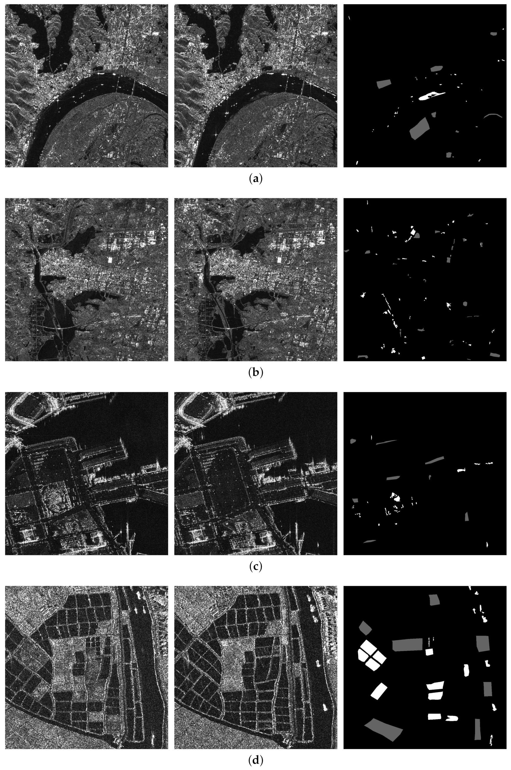
There are 4 SAR datasets in this experiment. (1) Huangshi dataset as shown in Figure 4a, Sentinel-1 SAR images in Huangshi Hubei, China acquired on 8 October 2014 and 19 December 2014. The spatial resolution is 5 m and image size is 1024 × 1024. (2) Daye dataset in Figure 4b, Sentinel-1 SAR images in Daye Hubei, China acquired on 8 October 2014 and 19 December 2014 with image size of 1024 × 1024. (3) San Francisco dataset in Figure 4c, TerraSAR images in San Francisco, America acquired on 5 December 2007 and 16 December 2007. The spatial resolution is 1m and image size is 1024 × 1024. (4) Guangdong dataset in Figure 4d, TerraSAR images in Guangdong, China acquired on 24 May 2008 and 19 December 2008 with image size of 1024 × 1024. The corresponding ground truth maps are labeled manually, as shown on the right of Figure 4.

In order to verify the validity of our proposed method, five metrics are computed to quantitatively investigate the detection results, i.e., Precision (P), Recall (R), Overall accuracy ($OA$), $Kappa$ coefficient and $F_1$.

$$P=\frac{TP}{TP+FP}$$

(9)

$$R=\frac{TP}{TP+FN}$$

(10)

$$F_1=\frac{2PR}{P+R}$$

(11)

$$OA=\frac{TP+TN}{TP+TN+FP+FN}$$

(12)

$$Kappa=\frac{OA-p_e}{1-p_e}$$

(13)

where $TP$, $FP$, $TN$ and $FN$ denote the number of true positives, the number of false positives, the number of true negatives and the number of false negatives respectively, as defined in

Table 1. Confusion matrix of change detection results.

	0 (Unchange, Prediction)	1 (Change, Prediction)
0 (unchange, ground truth)	$TP$	$FN$
1 (change, ground truth)	$FP$	$TN$

.

4.2. Analysis of Parameter Setting

As described in Section 3, the hyperparameters are selected before performing the proposed network, i.e., the number of hidden neurons in the AE-like network, the number of layers of the AE-like network and the weights in the loss. The efficiency of learning features may be affected by the number of hidden neurons and the number of hidden layers. The weights in the loss function can reflect the influence of the relation between different constraints and objective functions on the detection results. Thus, comparison experiments have been launched here to investigate the proper hyperparameter setting. Besides, there is a strong link between patch size and image resolution or the size of changed regions. Considering the SAR datasets tested in our exeriments, we choose the patch size as 5 × 5 by some comparative experiments and keep this patch size in the following experiments.

4.2.1. Number of Hidden Layers and Hidden Neurons

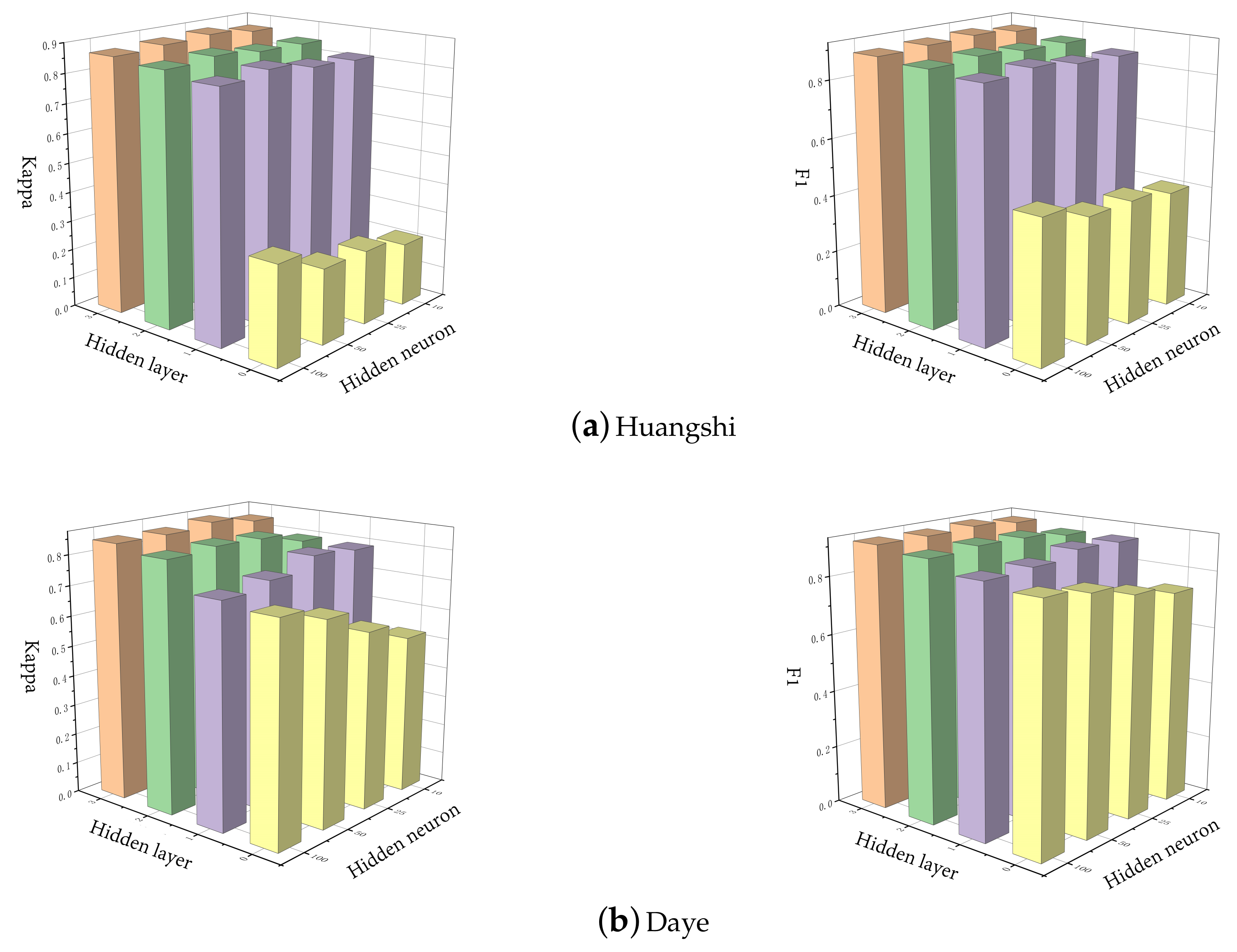
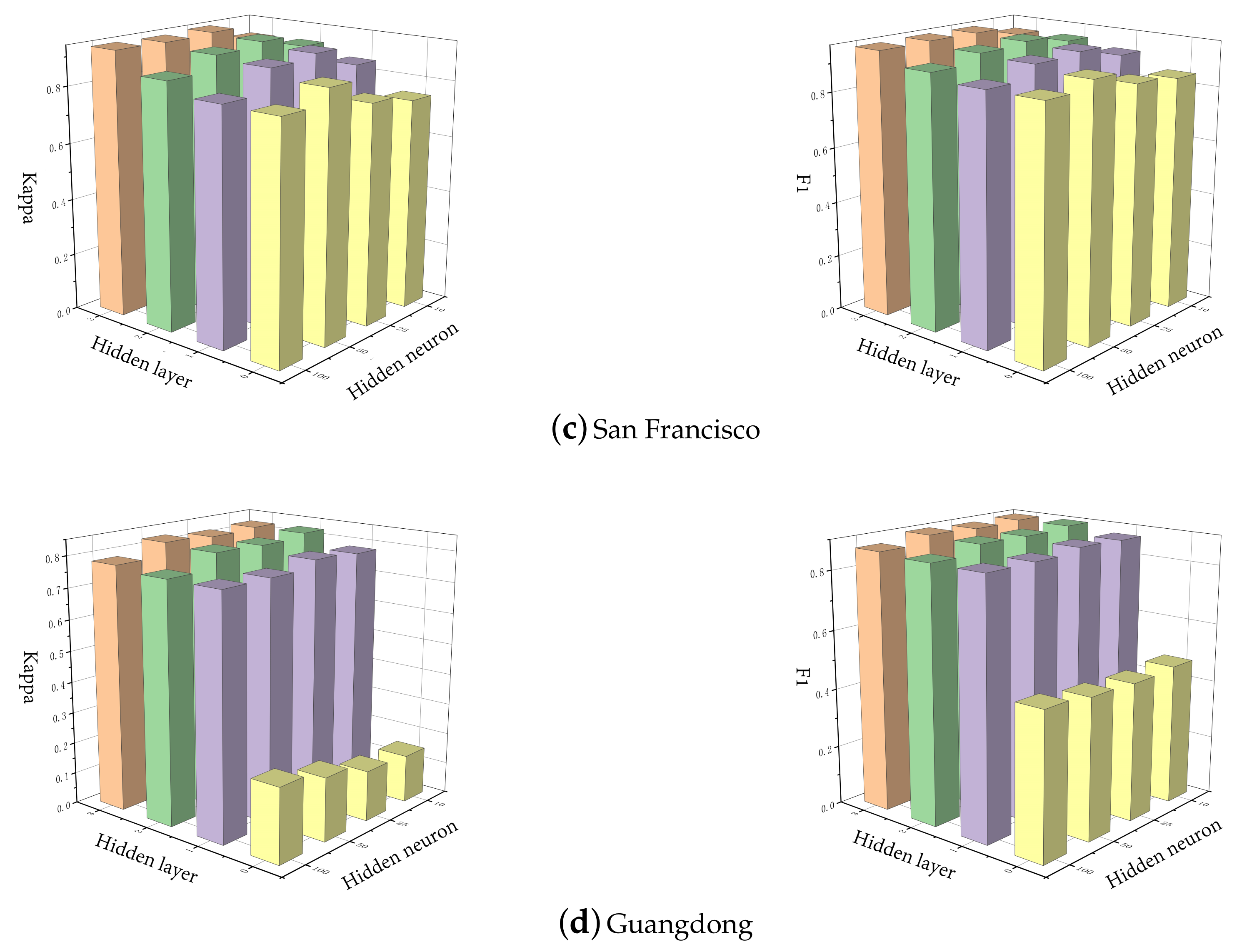
We argue that the number of hidden layers and the number of hidden neurons interact with each other. To choose the parameters of the network, we adopt a grid search method to avoid blindness and randomness, i.e., the number of hidden layers $\{0,1,2,3\}$ and the number of hidden neurons $\{10,25,50,100\}$. The weights in the loss function are ${\lambda }_1=1.0,{\lambda }_2=1.0$. The results are evaluated by Kappa and $F_1$.

The change detection performance against the number of non-linear hidden layers and hidden neurons in the AE-like network is shown in Figure 5. It can be seen that the detection accuracy significantly increases with the introduce of the non-linearly mapping by the AE-like network. In addition, the accuracy of change detection gradually increases with the increasing layers. It can be seen that the number of neurons in the hidden layers has a slight effect on the detection results. Consequently, in the following experiments, we perform the AE-like network with 3 hidden layers and 25 hidden neurons by balancing the detection accuracy and the computation complexity.

4.2.2. Weights in the Loss

The proposed loss in Equation (6) consists of the representation differential term, the data normalization term and the weight regularization term. The weights $\mathbf{\Lambda }=\{{\lambda }_1,{\lambda }_2\}$ control the balance among these terms. We test the DDSR network with ${\lambda }_1=\{10.0,1.0,0.1,0.01\}$ and ${\lambda }_2=\{10.0,1.0,0.1,0.01\}$.

Table 2. Change detection results of Huangshi dataset with different weights in the loss function.

Weights	${\mathit{\lambda }}_2=10.0$		${\mathit{\lambda }}_2=1.00$		${\mathit{\lambda }}_2=0.10$		${\mathit{\lambda }}_2=0.01$
	$\mathit{Kappa}$	$\mathit{F}\mathbf{1}$	$\mathit{Kappa}$	$\mathit{F}\mathbf{1}$	$\mathit{Kappa}$	$\mathit{F}\mathbf{1}$	$\mathit{Kappa}$	$\mathit{F}\mathbf{1}$
${\lambda }_1=10.0$	0.8656	0.8901	0.8694	0.8940	0.8378	0.8689	0.8618	0.8877
${\lambda }_1=1.00$	0.8651	0.8898	0.8822	0.9040	0.8503	0.8772	0.8347	0.8643
${\lambda }_1=0.10$	0.8602	0.8860	0.8167	0.8493	0.8176	0.8504	0.8617	0.8864
${\lambda }_1=0.01$	-	-	-	-	-	-	-	-

- denotes fail of the network training.

,

Table 3. Change detection results of Daye dataset with different weights in the loss function.

Weights	${\mathit{\lambda }}_2=10.0$		${\mathit{\lambda }}_2=1.00$		${\mathit{\lambda }}_2=0.10$		${\mathit{\lambda }}_2=0.01$
	$\mathit{Kappa}$	$\mathit{F}\mathbf{1}$	$\mathit{Kappa}$	$\mathit{F}\mathbf{1}$	$\mathit{Kappa}$	$\mathit{F}\mathbf{1}$	$\mathit{Kappa}$	$\mathit{F}\mathbf{1}$
${\lambda }_1=10.0$	0.8780	0.9315	0.8039	0.8931	0.8189	0.9027	0.8726	0.9307
${\lambda }_1=1.00$	0.8513	0.9188	0.8613	0.9237	0.8520	0.9189	0.8433	0.9116
${\lambda }_1=0.10$	0.8398	0.9118	0.8618	0.9229	0.8614	0.9222	0.8811	0.9338
${\lambda }_1=0.01$	-	-	-	-	-	-	-	-

- denotes fail of the network training.

,

Table 4. Change detection results of San Francisco dataset with different weights in the loss function.

Weights	${\mathit{\lambda }}_2=10.0$		${\mathit{\lambda }}_2=1.00$		${\mathit{\lambda }}_2=0.10$		${\mathit{\lambda }}_2=0.01$
	$\mathit{Kappa}$	$\mathit{F}\mathbf{1}$	$\mathit{Kappa}$	$\mathit{F}\mathbf{1}$	$\mathit{Kappa}$	$\mathit{F}\mathbf{1}$	$\mathit{Kappa}$	$\mathit{F}\mathbf{1}$
${\lambda }_1=10.0$	0.9170	0.9474	0.9159	0.9462	0.9135	0.9452	0.9317	0.9564
${\lambda }_1=1.00$	0.9150	0.9458	0.9377	0.9601	0.9278	0.9538	0.9366	0.9595
${\lambda }_1=0.10$	0.9157	0.9465	0.9379	0.9603	0.9333	0.9574	0.8882	0.9295
${\lambda }_1=0.01$	-	-	-	-	-	-	-	-

- denotes fail of the network training.

and

Table 5. Change detection results of Guangdong dataset with different weights in the loss function.

Weights	${\mathit{\lambda }}_2=10.0$		${\mathit{\lambda }}_2=1.00$		${\mathit{\lambda }}_2=0.10$		${\mathit{\lambda }}_2=0.01$
	$\mathit{Kappa}$	$\mathit{F}\mathbf{1}$	$\mathit{Kappa}$	$\mathit{F}\mathbf{1}$	$\mathit{Kappa}$	$\mathit{F}\mathbf{1}$	$\mathit{Kappa}$	$\mathit{F}\mathbf{1}$
${\lambda }_1=10.0$	0.7722	0.8661	0.7912	0.8776	0.8159	0.8924	0.7943	0.8796
${\lambda }_1=1.00$	0.8181	0.8935	0.8156	0.8915	0.8247	0.8974	0.8231	0.8964
${\lambda }_1=0.10$	-	-	-	-	-	-	-	-
${\lambda }_1=0.01$	-	-	-	-	-	-	-	-

- denotes fail of the network training.

list the $Kappa$ and $F_1$ of change detection results on dataset Huangshi, Daye, San Francisco and Guangdong. It can be found that ${\lambda }_1$ and ${\lambda }_2$ have great influence on the change detection results. Extremely small ${\lambda }_1$ tends to neglect the variance constraints, which leads to failure of the network training (output the zero weights ${\mathbf{W}}_{\mathrm{AE}}=0,{\mathbf{W}}_{\mathrm{SE}}=0$). Extremely small ${\lambda }_2$ stands for despising the covariance constraints. There will be lots of redundancy information among the channels of the output. The change detection results may drop up to 5% in terms of $Kappa$ and $F_1$, given unbalanced settings of ${\lambda }_1$ and ${\lambda }_2$. However, this dropping only takes place at the extreme cases, e.g., $\{{\lambda }_1=10,{\lambda }_2=0.01\}$ and $\{{\lambda }_1=0.1,{\lambda }_2=10\}$. ${\lambda }_1=1.0$ and ${\lambda }_2=1.0$ thus have been chosen in the proposed experiments.

4.3. Parameter Setting and Comparison Methods

In order to verify the superiority and efficiency of our proposed method, different change detection approaches are tested as reference methods in this experiment, i.e., (1) the classic mean ratio operator (MR) [1], (2) NORCAMA [25], a generalized likelihood ratio test based change criterion, (3) SAE + FCM + CNN [30], deep features based change detction. In our proposed approach, we convert each 5 × 5 patch into a vector as the input of our network. The number of neurons in the 3 non-linear AE-like network is 25. Consequently, the number of neurons in the self-expressive layer is 25 as well. The weights in the loss are ${\lambda }_1=1.0$ and ${\lambda }_2=1.0$.

4.4. Experimental Results

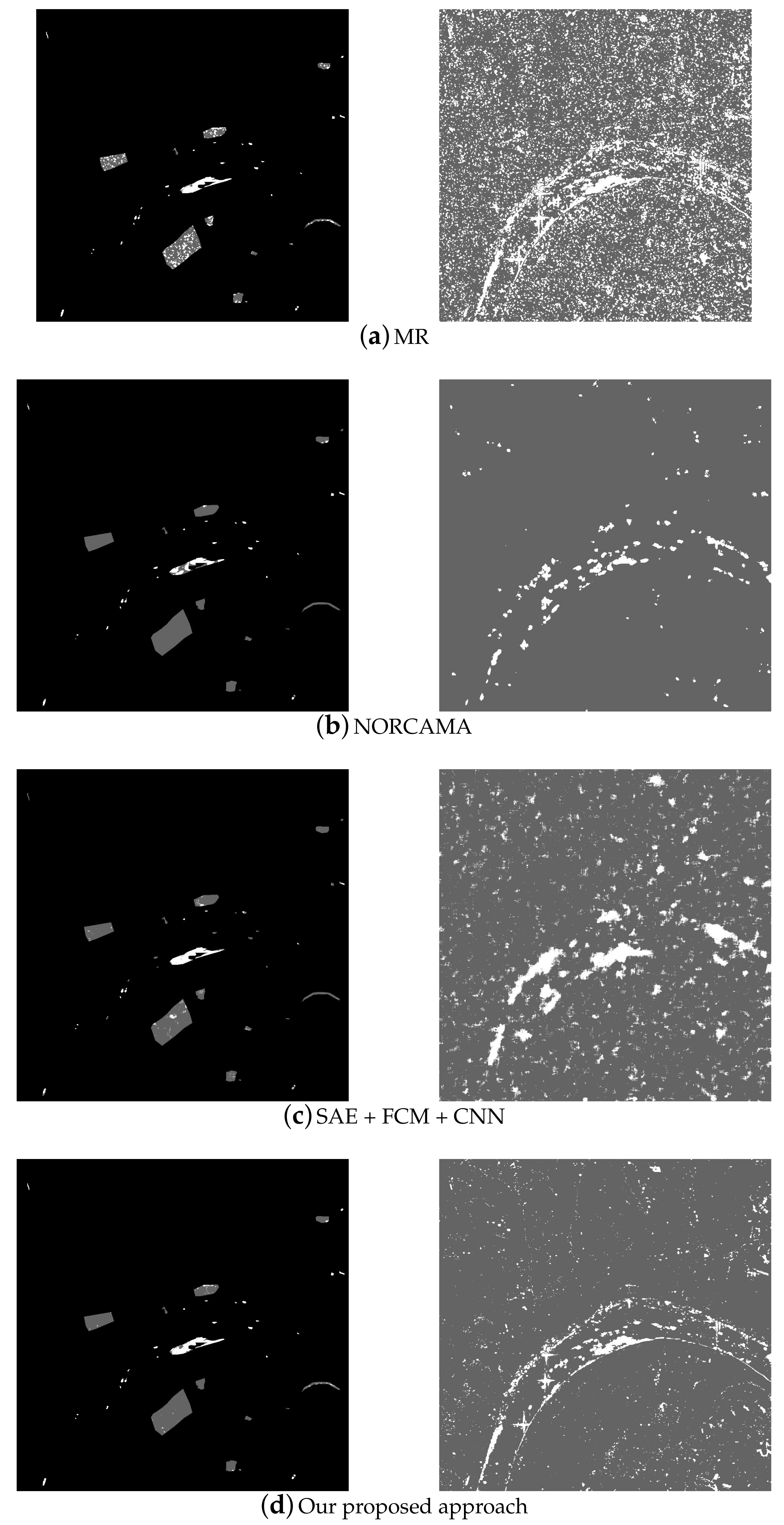
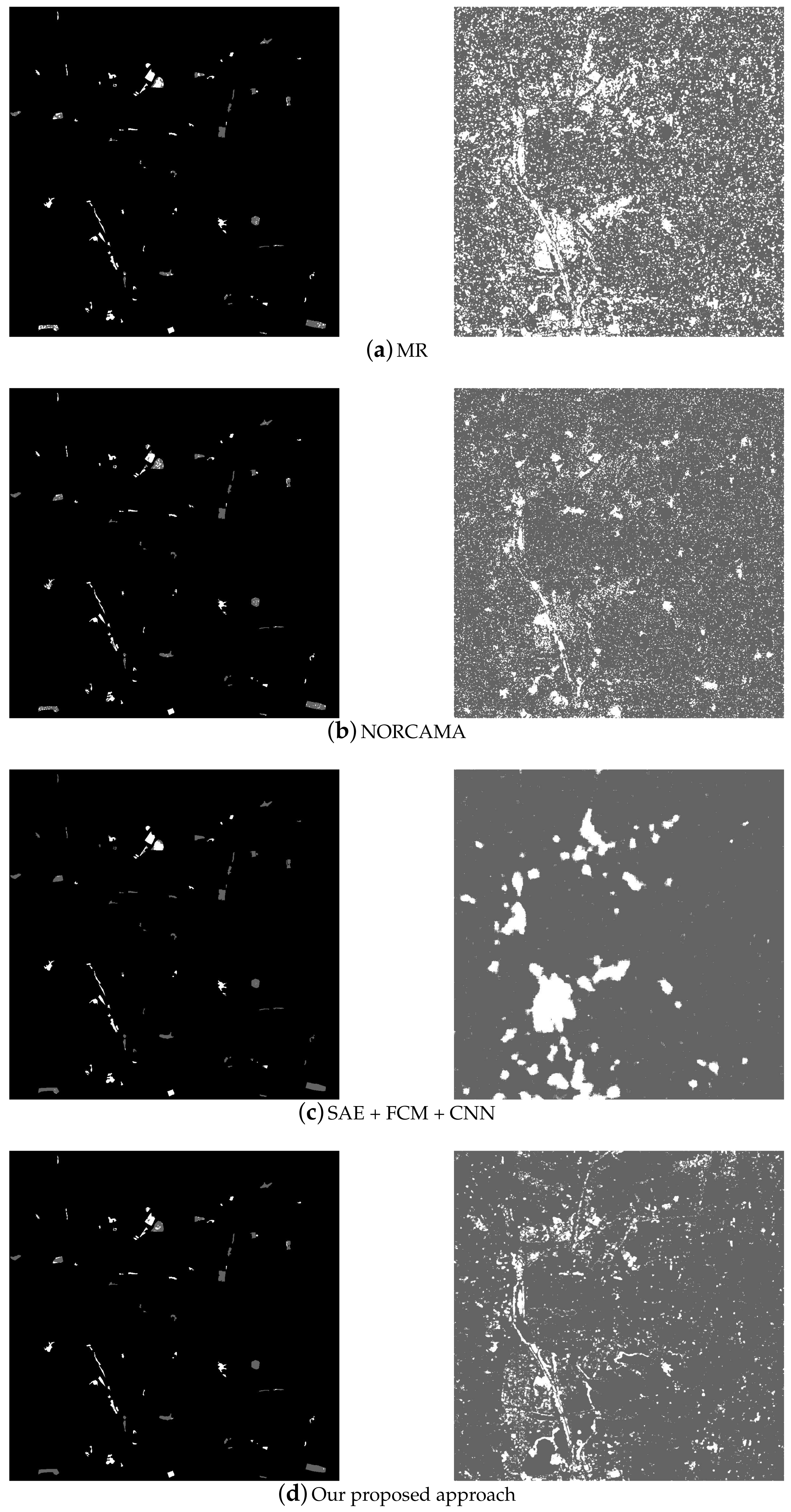
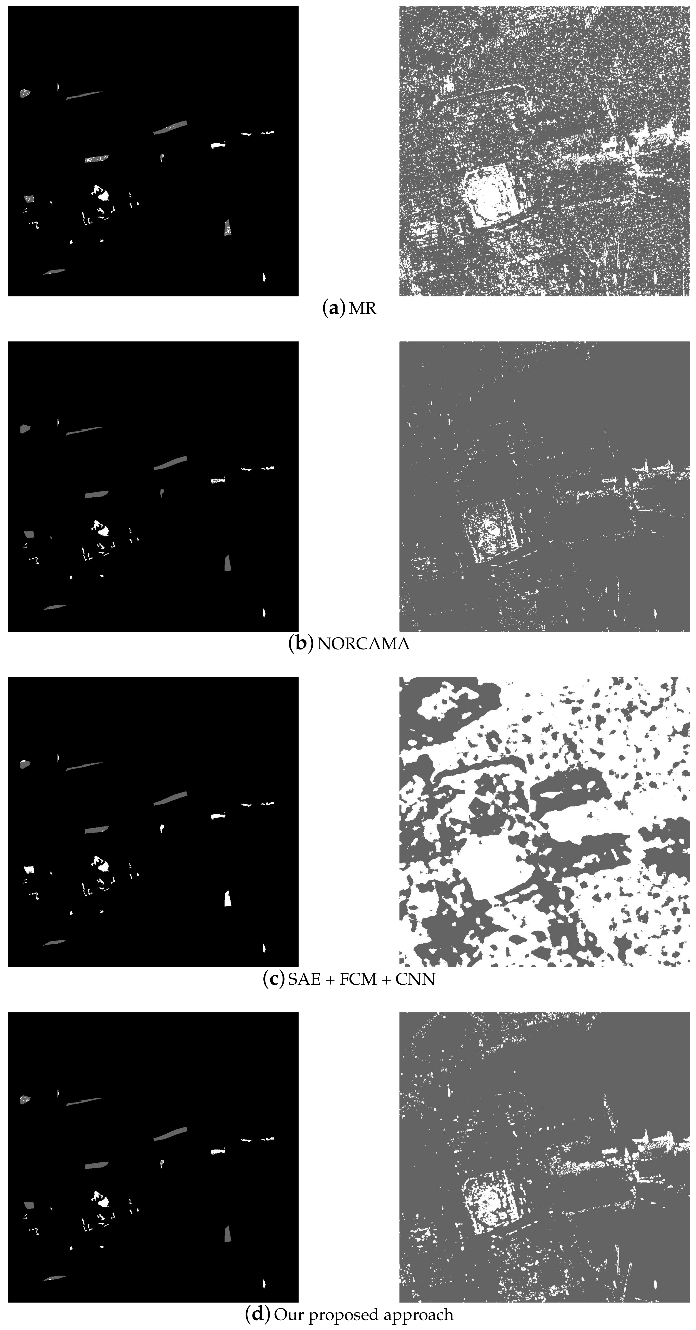
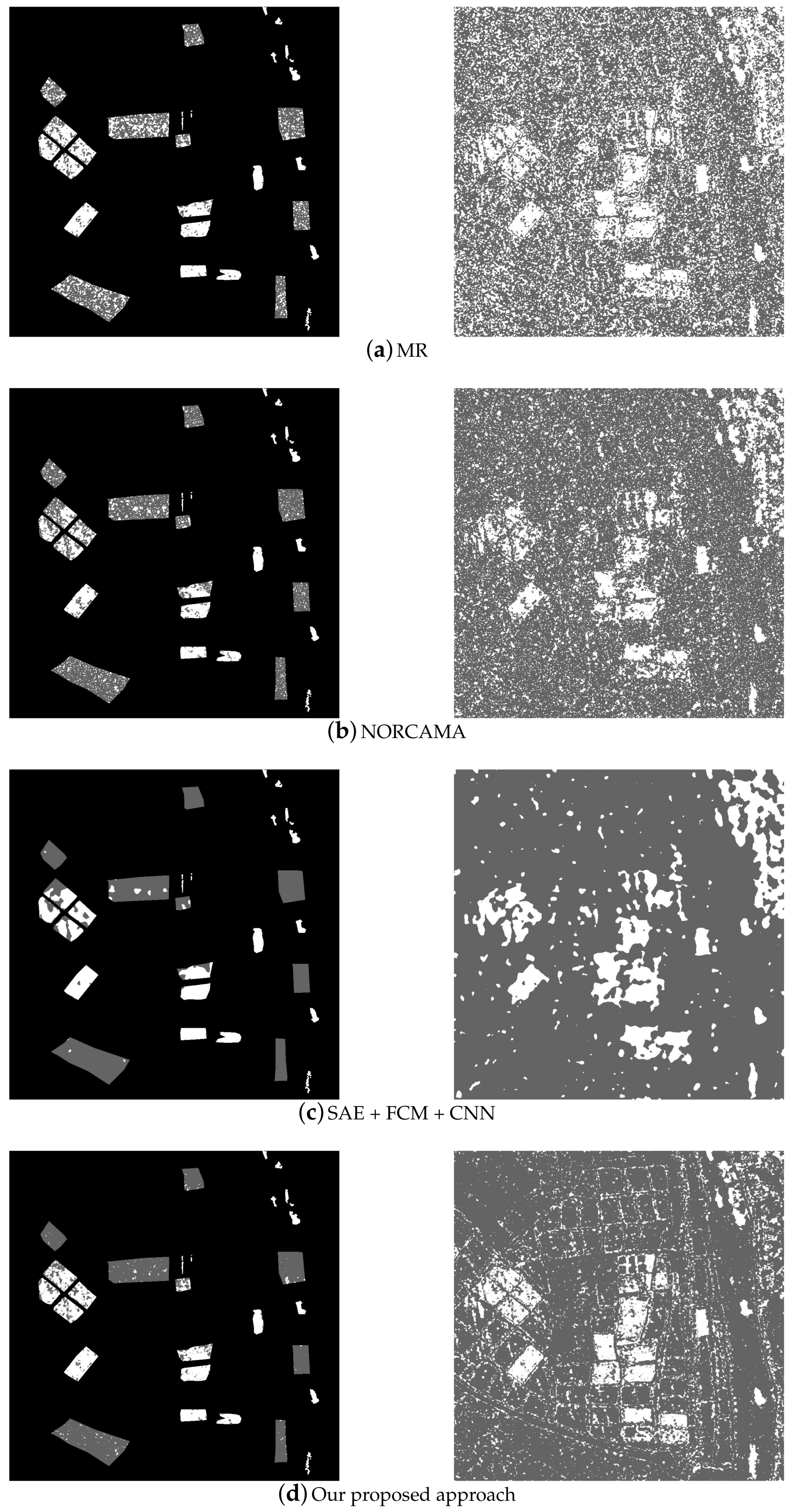
The change detection maps are shown in Figure 6, Figure 7, Figure 8 and Figure 9 and the quantitative metrics are presented in

Table 6. Change detection results of Huangshi dataset (The bold denotes the best results).

	TP	FN	FP	TN	OA	Kappa	P	R	F1
MR	14153	161	3988	3987	0.8139	0.5468	0.4999	0.9612	0.6578
NORCAMA	18023	1240	118	2908	0.9391	0.7755	0.9610	0.7011	0.8107
SAE + FCM + CNN	17506	816	635	3332	0.9349	0.7814	0.8399	0.8033	0.8212
Proposed approach	17773	423	368	3725	0.9645	0.8822	0.8980	0.9101	0.9040

,

Table 7. Change detection results of Daye dataset (The bold denotes the best results).

	TP	FN	FP	TN	OA	Kappa	P	R	F1
MR	5897	153	1733	6029	0.8635	0.7304	0.7767	0.9753	0.8647
NORCAMA	6863	882	767	5300	0.8806	0.7581	0.8736	0.8573	0.8654
SAE + FCM + CNN	6873	1361	757	4821	0.8467	0.6870	0.8643	0.7798	0.8199
Proposed approach	7122	440	508	5742	0.9314	0.8613	0.9187	0.9288	0.9237

,

Table 8. Change detection results of San Francisco dataset (The bold denotes the best results).

	TP	FN	FP	TN	OA	Kappa	P	R	F1
MR	6594	5	746	4007	0.9338	0.8611	0.8430	0.9988	0.9143
NORCAMA	7333	474	7	3538	0.9576	0.9048	0.9980	0.8819	0.9364
SAE + FCM + CNN	5399	0	1941	4012	0.8290	0.6629	0.6739	1.00	0.8052
Proposed approach	7103	89	237	3923	0.9713	0.9377	0.9430	0.9778	0.9601

and

Table 9. Change detection results of Guangdong dataset (The bold denotes the best results).

	TP	FN	FP	TN	OA	Kappa	P	R	F1
MR	37412	7262	16287	35749	0.7565	0.5171	0.6870	0.8312	0.7522
NORCAMA	45422	11957	8277	31054	0.7908	0.5727	0.7896	0.7220	0.7543
SAE + FCM + CNN	52679	8173	1020	34838	0.9049	0.8043	0.9716	0.8100	0.8834
Proposed approach	52325	7313	1374	35698	0.9102	0.8156	0.9629	0.8300	0.8915

. From the results, we can find that the classic MR has noisy detection results and the corresponding detection accuracy is lower than other approaches. NORCAMA with the help of pre-denoising operation yields less noisy detection results, however, its detection accuracy is highly depending on the pre-denoising performance. SAE + FCM + CNN achieves a balance between the precision and the recall, which has less noise than the classic MR. However, it heavily relies on the pseudo labels, which may make the final detection accuracy very low when the pre-detection/classification results are poor. The edges of the detection results are very indistinct. Generally, our DDSR network outperforms the reference methods with higher detection accuracy, smooth detection results and clear edges.

5. Conclusions

In this paper, we present a differentially deep subspace representation (DDSR) for bi-temporal SAR images change detection. The proposed architecture consists of an autoencoder-like (AE-like) non-linear mapping network, a self-expressive linear transforming layer and a K-Means cluster. Contrary to the deep subspace clustering algorithms, our DDSR representation focuses on the change detection task (the comparison of two input image patches) instead of the efficient representation of the input data. The classic AE network has been modified to an AE-like architecture by training to minimize the differential representation of the unchanged pixel pairs without the traditional reconstruction error, i.e., the decoder has been discarded. The input bi-temporal SAR data is first non-linearly mapped to a lower-dimensional latent space by the proposed AE-like network. To better distingue the changed and unchanged pixels, a self-expressive layer has been applied to linearly transform the mapped SAR data to a subspace. The final change criterion is the difference between the subspace representations of the two temporal images. The classic K-Means is applied to identify the changed pixels. The experimental results have demonstrated that our proposed method yields better performance in terms of detection accuracy on the real SAR datasets than the reference methods. Future work could focus on the extensions of our DDSR to optical and SAR image change detection.

References

- Singh, A. Review article digital change detection techniques using remotely-sensed data. Int. J. Remote Sens. 1989, 10, 989–1003. [Google Scholar] [CrossRef]
- Wessels, K.; Van Den Bergh, F.; Roy, D.; Salmon, B.P.; Steenkamp, K.C.; MacAlister, B.; Swanepoel, D.; Jewitt, D. Rapid land cover map updates using change detection and robust random forest classifiers. Remote Sens. 2016, 8, 888. [Google Scholar] [CrossRef]
- Brunner, D.; Lemoine, G.; Bruzzone, L. Earthquake damage assessment of buildings using VHR optical and SAR imagery. IEEE Trans. Geosci. Remote Sens. 2010, 48, 2403–2420. [Google Scholar] [CrossRef]
- Taubenbock, H.; Esch, T.; Felbier, A.; Wiesner, M.; Roth, A.; Dech, S. Monitoring urbanization in mega cities from space. Remote Sens. Environ. 2012, 117, 162–176. [Google Scholar] [CrossRef]
- Noordermeer, L.; Okseter, R.; Orka, H.O.; Gobakken, T.; Næsset, E.; Bollandsås, O.M. Classifications of Forest Change by Using Bitemporal Airborne Laser Scanner Data. Remote Sens. 2019, 11, 2145. [Google Scholar] [CrossRef]
- Bovolo, F.; Bruzzone, L. A theoretical framework for unsupervised change detection based on change vector analysis in the polar domain. IEEE Trans. Geosci. Remote Sens. 2006, 45, 218–236. [Google Scholar] [CrossRef]
- Xu, R.; Lin, H.; Lu, Y.; Luo, Y.; Ren, Y.; Comber, A. A modified change vector approach for quantifying land cover change. Remote Sens. 2018, 10, 1578. [Google Scholar] [CrossRef]
- Liu, S.; Bruzzone, L.; Bovolo, F.; Zanetti, M.; Du, P. Sequential spectral change vector analysis for iteratively discovering and detecting multiple changes in hyperspectral images. IEEE Trans. Geosci. Remote Sens. 2015, 53, 4363–4378. [Google Scholar] [CrossRef]
- Wold, S.; Esbensen, K.; Geladi, P. Principal component analysis. Chemom. Intell. Lab. Syst. 1987, 2, 37–52. [Google Scholar] [CrossRef]
- Atasever, U.H.; Kesikoglu, M.H.; Ozkan, C. A new artificial intelligence optimization method for PCA based unsupervised change detection of remote sensing image data. Neural Netw. World 2016, 26, 141. [Google Scholar] [CrossRef]
- Wang, C.; Xiao, Y.; Liu, B.; Du, D.; Luo, R. An Improved Change Detection Based on PCA and FCM Clustering for Earthen Ruins. In Advanced Multimedia and Ubiquitous Engineering; Springer: Singapore, 2019; pp. 28–35. [Google Scholar]
- Levien, L.M.; Fischer, C.S.; Roffers, P.D.; Maurizi, B.; Suero, J.; Huang, X. A machine-learning approach to change detection using multi-scale imagery. In Proceedings of the ASPRS Annual Conference, Portland, OR, USA, 20 May 1999; American Society for Photogrametry and Remote Sensing (ASPRS): Bethesda, MD, USA, 1999; Volume 1, p. 22. [Google Scholar]
- Collins, J.B.; Woodcock, C.E. An assessment of several linear change detection techniques for mapping forest mortality using multitemporal Landsat TM data. Remote Sens. Environ. 1996, 56, 66–77. [Google Scholar] [CrossRef]
- Rosa RA, S.; Fernandes, D.; Nogueira, J.B.; Wimmer, C. Automatic change detection in multitemporal X-and P-band SAR images using Gram-Schmidt process. In Proceedings of the 2015 IEEE International Geoscience and Remote Sensing Symposium (IGARSS), Milan, Italy, 26–31 July 2015; pp. 2797–2800. [Google Scholar]
- Nielsen, A.A.; Conradsen, K.; Simpson, J.J. Multivariate alteration detection (MAD) and MAF postprocessing in multispectral, bitemporal image data: New approaches to change detection studies. Remote Sens. Environ. 1998, 64, 1–19. [Google Scholar] [CrossRef]
- Chen, Y.; Sun, K.; Li, D.; Bai, T.; Li, W. Improved relative radiometric normalization method of remote sensing images for change detection. J. Appl. Remote Sens. 2018, 12, 045018. [Google Scholar] [CrossRef]
- Xv, J.; Zhang, B.; Guo, H.; Lu, J.; Lin, Y. Combining iterative slow feature analysis and deep feature learning for change detection in high-resolution remote sensing images. J. Appl. Remote Sens. 2019, 13, 024506. [Google Scholar]
- Wu, C.; Du, B.; Zhang, L. Slow feature analysis for change detection in multispectral imagery. IEEE Trans. Geosci. Remote Sens. 2013, 52, 2858–2874. [Google Scholar] [CrossRef]
- Preiss, M.; Stacy, N.J.S. Coherent Change Detection: Theoretical Description and Experimental Results; Defence Science And Technology Organisation: Edinburgh, Australia, 2006. [Google Scholar]
- Rignot., E.J.M.; Van Zyl, J.J. Change detection techniques for ERS-1 SAR data. IEEE Trans. Geosci. Remote Sens. 1993, 31, 896–906. [Google Scholar] [CrossRef]
- Bazi, Y.; Bruzzone, L.; Melgani, F. An unsupervised approach based on the generalized Gaussian model to automatic change detection in multitemporal SAR images. IEEE Trans. Geosci. Remote Sens. 2005, 43, 874–887. [Google Scholar] [CrossRef]
- Bovolo, F.; Bruzzone, L. A detail-preserving scale-driven approach to change detection in multitemporal SAR images. IEEE Trans. Geosci. Remote Sens. 2005, 43, 2963–2972. [Google Scholar] [CrossRef]
- Lombardo, P.; Oliver, C.J. Maximum likelihood approach to the detection of changes between multitemporal SAR images. IEE Proc.-Radar Sonar Navig. 2001, 148, 200–210. [Google Scholar] [CrossRef]
- Quin, G.; Pinel-Puyssegur, B.; Nicolas, J.M.; Loreaux, P. MIMOSA: An automatic change detection method for SAR time series. IEEE Trans. Geosci. Remote Sens. 2013, 52, 5349–5363. [Google Scholar] [CrossRef]
- Su, X.; Deledalle, C.-A.; Tupin, F.; Sun, H. NORCAMA: Change analysis in SAR time series by likelihood ratio change matrix clustering. ISPRS J. Photogramm. Remote Sens. 2015, 101, 247–261. [Google Scholar] [CrossRef]
- Peng, D.; Zhang, Y.; Guan, H. End-to-End Change Detection for High Resolution Satellite Images Using Improved UNet++. Remote Sens. 2019, 11, 1382. [Google Scholar] [CrossRef]
- Ji, S.; Shen, Y.; Lu, M.; Zhang, Y. Building Instance Change Detection from Large-Scale Aerial Images using Convolutional Neural Networks and Simulated Samples. Remote Sens. 2019, 11, 1343. [Google Scholar] [CrossRef]
- Fang, B.; Pan, L.; Kou, R. Dual Learning-Based Siamese Framework for Change Detection Using Bi-Temporal VHR Optical Remote Sensing Images. Remote Sens. 2019, 11, 1292. [Google Scholar] [CrossRef]
- Saha, S.; Bovolo, F.; Bruzzone, L. Unsupervised Deep Change Vector Analysis for Multiple-Change Detection in VHR Images. IEEE Trans. Geosci. Remote Sens. 2019, 57, 3677–3693. [Google Scholar] [CrossRef]
- Gong, M.; Yang, H.; Zhang, P. Feature learning and change feature classification based on deep learning for ternary change detection in SAR images. ISPRS J. Photogramm. Remote Sens. 2017, 129, 212–225. [Google Scholar] [CrossRef]
- Hartigan, J.A.; Wong, M.A. Algorithm AS 136: A k-means clustering algorithm. J. R. Stat. Soc. Ser. C (Appl. Stat.) 1979, 28, 100–108. [Google Scholar] [CrossRef]
- Du, B.; Ru, L.; Wu, C.; Zhang, L. Unsupervised Deep Slow Feature Analysis for Change Detection in Multi-Temporal Remote Sensing Images. IEEE Trans. Geosci. Remote Sens. 2019. [Google Scholar] [CrossRef]
- Ji, P.; Zhang, T.; Li, H.; Salzmann, M.; Reid, I. Deep subspace clustering networks. In Proceedings of the 31st International Conference on Advances in Neural Information Processing Systems, Long Beach, CA, USA, 4–9 December 2017; pp. 24–33. [Google Scholar]
- Peng, X.; Feng, J.; Xiao, S.; Yau, W.; Zhou, J.T.; Yang, S. Structured autoencoders for subspace clustering. IEEE Trans. Image Process. 2018, 27, 5076–5086. [Google Scholar] [CrossRef]
- Wu, C.; Zhang, L.; Du, B. Kernel slow feature analysis for scene change detection. IEEE Trans. Geosci. Remote Sens. 2017, 55, 2367–2384. [Google Scholar] [CrossRef]
- Liwicki, S.; Zafeiriou, S.P.; Pantic, M. Online kernel slow feature analysis for temporal video segmentation and tracking. IEEE Trans. Image Process. 2015, 24, 2955–2970. [Google Scholar] [CrossRef] [PubMed]
- Zhang, H.; Tian, X.; Deng, X. Batch process monitoring based on multiway global preserving kernel slow feature analysis. IEEE Access 2017, 5, 2696–2710. [Google Scholar] [CrossRef]
Figure 1.
Deep networks in related works. (a) Deep subspace clustering [33]. (b) Deep slow feature analysis [32].
Figure 2.
The differentially deep subspace representation for synthetic aperture radar (SAR) image change detection. The network consists of an encoder with 3 layers (non-linear mapping), a self-expressive layer (linear transform) and a classic K-Means clustering.
Figure 3.
The encoder network diagram. (a) A simple encoder network consists of only an input layer, a hidden layer and an output layer. (b) A multi-layer encoder network including input layer, two hidden layers, output layer.
Figure 4.
Datasets tested in the experiments. (a) Huangshi dataset. (b) Daye dataset. (c) San Francisco dataset. (d) Guangdong dataset. From left to right, the bi-temporal SAR images and the corresponding reference change maps. In the reference change maps, the unchanged and changed pixels are gray and white respectively (black is not defined).
Figure 5.
The influence of the number of non-linear layers and hidden neurons in the AE-like network on the change detection results. The vertical axis represents the Kappa and F1 metrics of the detection results. One horizontal axis denotes the proposed network without the autoencoder (AE)-like network and with the AE-like network containing 1, 2 or 3 hidden layers, the other horizontal axis denotes the number of hidden neurons. Different colors denote different number of hidden layer. (a) Change detection results on Huangshi dataset. (b) Change detection results on Daye dataset. (c) Change detection results on San Francisco dataset. (d) Change detection results on Guangdong dataset. The left represents kappa metrics and the right denotes F1 metrics.
Figure 6.
Change detection results of Huangshi dataset by (a) mean ratio (MR), (b) NORCAMA, (c) SAE + FCM + CNN, (d) Our proposed approach. The left represents detection result with ground truth mask. The right denotes detection result without ground truth mask.
Figure 7.
Change detection results of Daye dataset by (a) MR, (b) NORCAMA, (c) SAE + FCM + CNN, (d) Our proposed approach. The left represents detection result with ground truth mask. The right denotes detection result without ground truth mask.
Figure 8.
Change detection results of San Francisco dataset by (a) MR, (b) NORCAMA, (c) SAE + FCM + CNN, (d) Our proposed approach. The left represents detection result with ground truth mask. The right denotes detection result without ground truth mask.
Figure 9.
Change detection results of Guangdong dataset by (a) MR, (b) NORCAMA, (c) SAE + FCM + CNN, (d) Our proposed approach. The left represents detection result with ground truth mask. The right denotes detection result without ground truth mask.