1. Introduction
Noctilucent clouds (NLC) that can be seen by the naked eye and polar mesospheric summer echoes (PMSE) observed with radar display the complex dynamics of the atmosphere at approximately 80 to 90 km height [
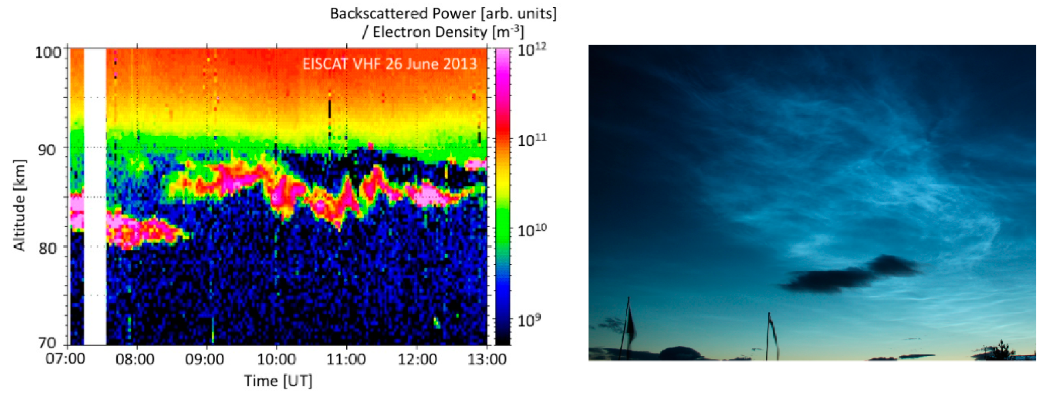
1]. PMSE and NLC display wavy structures (as shown
Figure 1) around the summer mesopause, a region that is highly dynamical with turbulent vortices and waves of scales from a few km to several thousand km. Analysis of these structures in the upper Earth atmosphere gives us information on the dynamics in this region.
Both the NLC and PMSE phenomena occur in the presence of ice particles. The topic of ice particle formation and its link to climate change is currently in debate in the atmospheric community and needs further investigation. Recent model results [
2] suggest a significant increase in the NLC occurrence number and NLC brightness over the period 1960–2008 and its link to the increase of water vapor as a result of the increasing methane content in the mesosphere. At the same time, actual ground-based NLC observations show about zero or small, statistically insignificant trends in the NLC occurrence frequency and brightness for the past five decades [
1,
3,
4,
5,
6,
7]. The time-series analyses of satellite observations in combination with model calculations indicate that the cloud frequencies are influenced by factors like stratospheric temperature, volcanic activity, and solar cycle [
8,
9]. In this context the comparison of NLC and PMSE will also improve the understanding of their formation processes.
Figure 1.
The polar mesospheric summer echoes (PMSE) radar echoes associated with polar ice clouds on the left [
10] and optical image of Noctilucent clouds (NLC) on the right.
Figure 1.
The polar mesospheric summer echoes (PMSE) radar echoes associated with polar ice clouds on the left [
10] and optical image of Noctilucent clouds (NLC) on the right.
The morphological shape of the clouds indicates the influence of wave propagation of various scales. Proper description and comparison of cloud structure is a step toward a detailed analysis of the role of atmospheric waves in the formation of PMSE and NLC. Both PMSE and NLC are observed during summer for several months, hence, large data sets are available for statistical analysis of the structures. A series of observations were made to collect optical images and radar data in common or overlapping volumes of the summer mesopause. So far only a few of the common volume observations were successful. In order to do a detailed analysis of the morphological shapes, advanced methods are required.
As a first step towards an integrated statistical analysis, we propose a framework for the analysis of NLC observation. The paper is organized as follows: in
Section 2, we discuss the theory behind the polar mesospheric summer echoes and noctilucent clouds, and outline our proposed framework for analysis of NLC and PMSE. Next, in
Section 3, we discuss the methodology behind the analysis of noctilucent clouds, the dataset, procedure used, and the methods employed for the analysis. In
Section 4, we discuss the results obtained from the comparison of different methods used in this paper. Finally, in
Section 5, we briefly discuss the results and outline strategies for future research directions.
2. Theory and Motivation
In this section, we discuss the theory behind NLC and PMSE and outline the proposed framework for their analysis.
2.1. Noctilucent Clouds and Polar Mesospheric Summer Echoes
The mesopause is the upper boundary of the mesosphere, the region of the atmosphere that is characterized by decreasing temperature with increasing altitude. The atmospheric temperature has its minimum at the mesopause and then increases with height again in the thermosphere lying above. The mesosphere and lower thermosphere are strongly influenced by atmospheric waves that couple the region to lower and higher layers. The waves determine the dynamical and thermal state of the atmosphere. They connect atmospheric regions from the ground to the lower thermosphere (0–130 km) and determine general atmospheric circulation by transferring their energy and momentum flux to the mean flow. The pronounced example of action of gravity waves (GWs) is the formation of the extremely cold polar summer mesopause (80–90 km) where the temperatures fall to the lowest values of the entire terrestrial atmosphere. Generated normally in the troposphere, gravity waves on the way up experience filtering (absorption) by zonal wind in the mesosphere [
11]. The rest propagates further and grow in amplitude as atmospheric density exponentially decreases. The waves with large amplitudes break at the mesospheric altitudes or higher up and exert drag on the mean flow. This gives rise to a meridional flow from the summer to winter mesosphere. As a result, global circulation from the winter to the summer poles moves air masses downward at the winter pole and upward at the summer pole. Hence, adiabatic cooling lowers the mesopause temperature in summer at the mid and high latitudes [
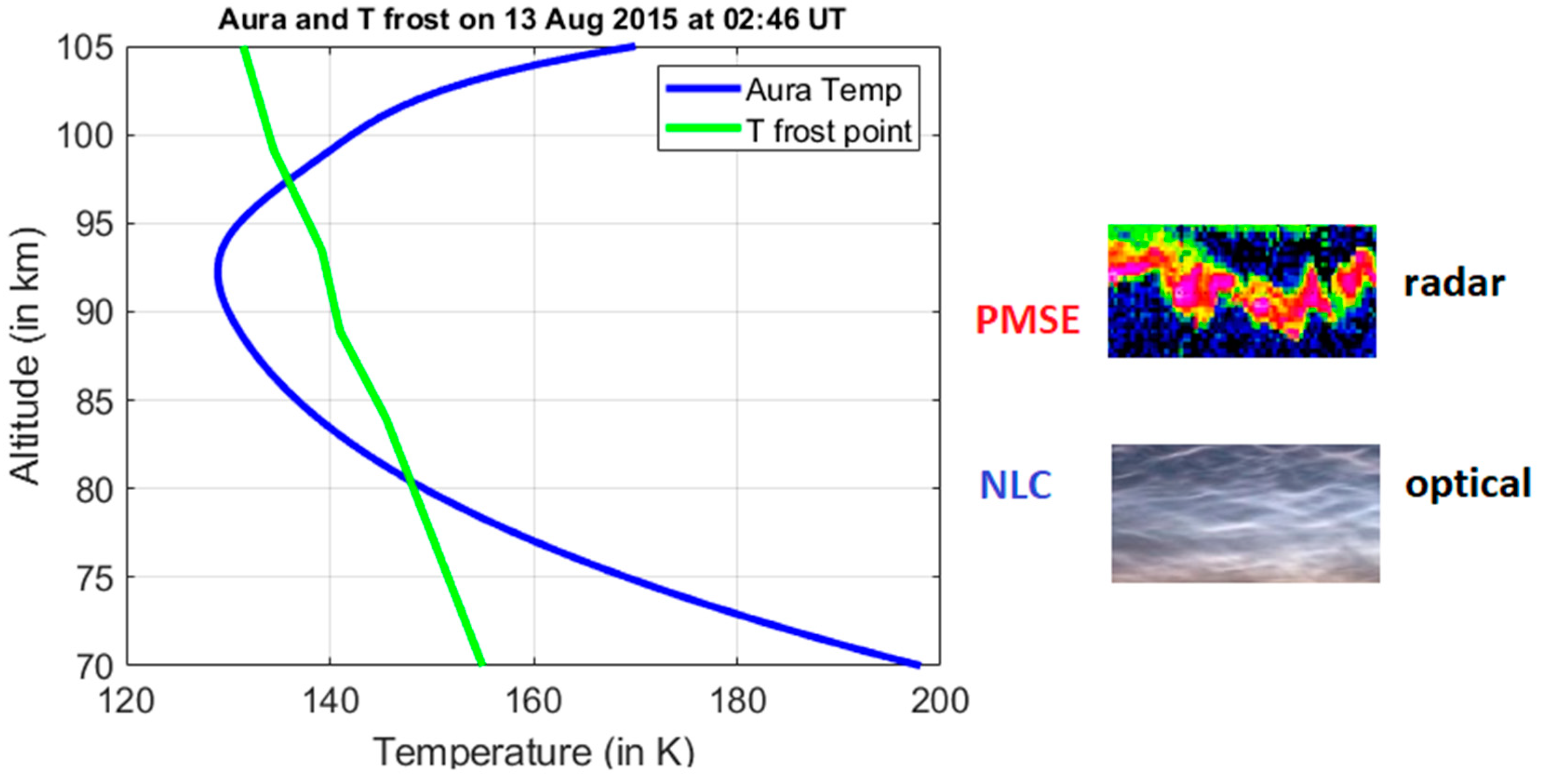
12]. There is also a strong influence of planetary waves on global scales as well as of turbulent eddies of a few meters. This dynamical forcing drives the polar summer mesosphere to around 60 degrees below radiative equilibrium temperatures. The temperature drops below the frost temperature (please see
Figure 2) and clouds of ice particles, polar mesospheric clouds (PMC) form at heights 80 to 85 km [
9]. Some of the PMC are visible to the eye after sunset when the atmosphere below is not illuminated by the Sun, those are the NLC. At similar, overlapping altitudes, the PMSE are observed [
13]. NLC form by light scattering at ice particles. PMSE are influenced by neutral atmospheric dynamics, turbulence, and dusty plasma effects, and their exact formation conditions are still subject to investigations [
14].
The conditions when wave dynamics cools the air down to 130 K and less so that small water-ice particles form prevail during the summer months and at high- and mid-latitude. PMSE ice particles are smaller in size (5–30 nm) and lighter compared to heavier NLC particles of 30–100 nm [
17]. That is why a PMSE layer usually resides above an NLC layer. Ground-based optical imagers and lidars can detect an NLC layer due to Mie scattering of sunlight on larger ice particles while VHF and UHF radars can detect a PMSE layer by means of radio waves scattering from fluctuations in electron density (at half-radar wavelength) that move with a neutral wind, which, in turn, can be modulated by waves. Future detailed comparison of both phenomena would provide valuable information both on the atmospheric structure and on the formation of the ice particles. It should be noted that NLC describes the variation of the atmospheric layer on spatial horizontal scales, while PMSE observations describe the radar echoes at a given location and their time variation which further complicates the analysis. Using high-power, large-aperture radar for the PMSE observations has the advantage that those radar also measure incoherent scatter in the vicinity of the PMSE and thus provide information on the ionospheric and dusty plasma conditions [
18].
2.2. Proposed Framework
EISCAT is an international research infrastructure for collecting radar observations and using incoherent scatter technique for studying the atmosphere and near-Earth space environment [
19]. The EISCAT_3D infrastructure is currently under development and will comprise five phased-array antenna fields located in different locations across Finland, Norway, and Sweden, each with around 10,000 dipole antenna elements [
19]. One of these locations will be used to transmit radio waves at 233 MHz, and all five locations will have receivers to measure the returned radio signals [
19]. As radio waves accelerate or heat electrons and ions in the upper atmosphere, the interactions of electromagnetic waves with the charged particles can be used to understand the properties of the near-Earth space environment [
20]. The measurements in the mesosphere reveal PMSE as well as basic plasma parameters.
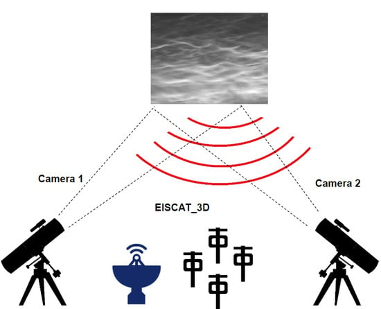
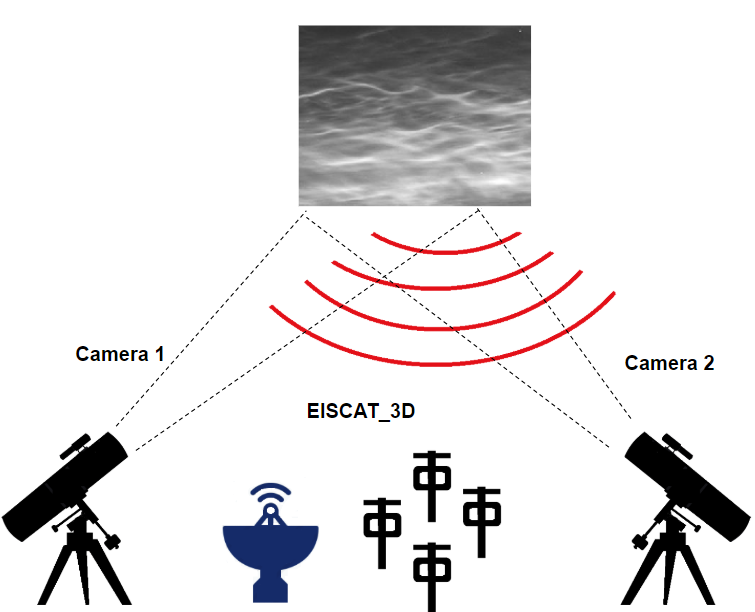
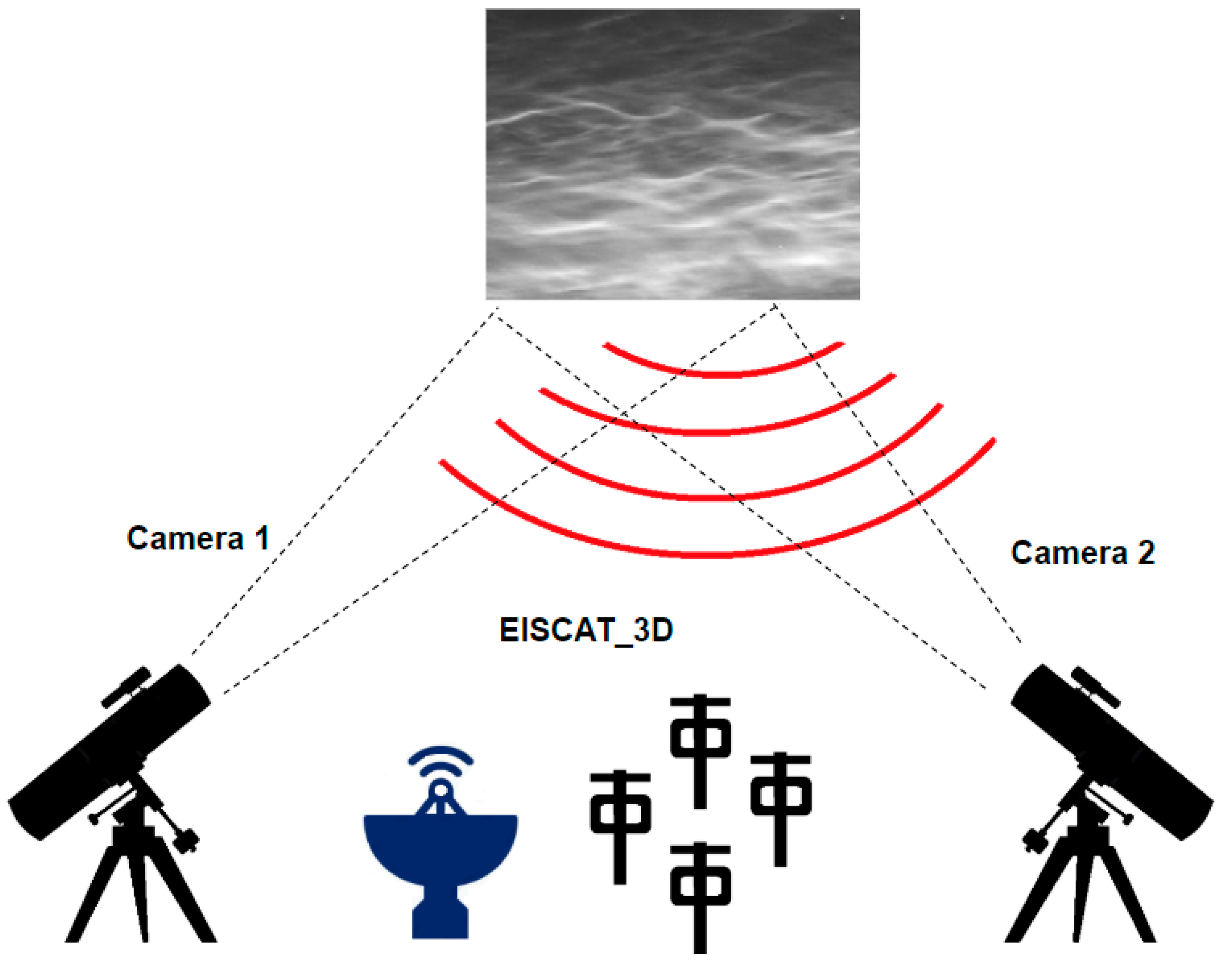
In the proposed framework as shown in
Figure 3, the main idea is to use cameras to detect noctilucent cloud activity in the atmosphere and use the associated timestamps to synchronize the optical observations with that of radar data obtained by using EISCAT. By synchronizing the radar data with optical images we can get a detailed understanding of the conditions leading to the formation of noctilucent clouds, and their propagation and dynamics in 3D space.
As an example, it is possible to carry out summer observation campaigns to study PMSE and NLC activity in the common volume of the atmosphere above the Tromsø EISCAT station. As EISCATradars are operating near Tromsø, two optical automated cameras, located at Kiruna (Sweden) and Nikkaluokta (Sweden), can register the potential occurrence of NLCs above the radar site. Both locations of the NLC cameras are about 200 km south of Tromsø, which permits making NLC triangulation measurements and hence estimating NLC height and dynamics in 3D space. After that, the observations pertaining to PMSE layers can be compared to those of the NLC to estimate characteristics of the gravity waves.
3. Methodology
In this section, we specify the dataset used for our experiments, discuss the procedure used for the analysis of the dataset and elaborate on the different methods used for the analysis.
3.1. Dataset
The dataset comprises of images captured from three different locations: Kiruna, Sweden (67.84°N, 20.41°E), Nikkaluokta, Sweden (67.85°N, 19.01°E), and Moscow, Russia (56.02°N, 37.48°E), during NLC activity. The images reflect the different conditions: low contrast or faint NLC activity, strong NLC activity, tropospheric clouds, and a combination of these conditions. Please note that while the two locations in Sweden are a part of the proposed framework, the data gathered from Moscow was mainly used to train and test for different challenging conditions associated with the NLC activity.
3.2. Procedure
First, an input image (typically of size 3456 by 2304 pixels) is resized to one-quarter of the original size. Downsampling an image helps to reduce the computational complexity of analysis.
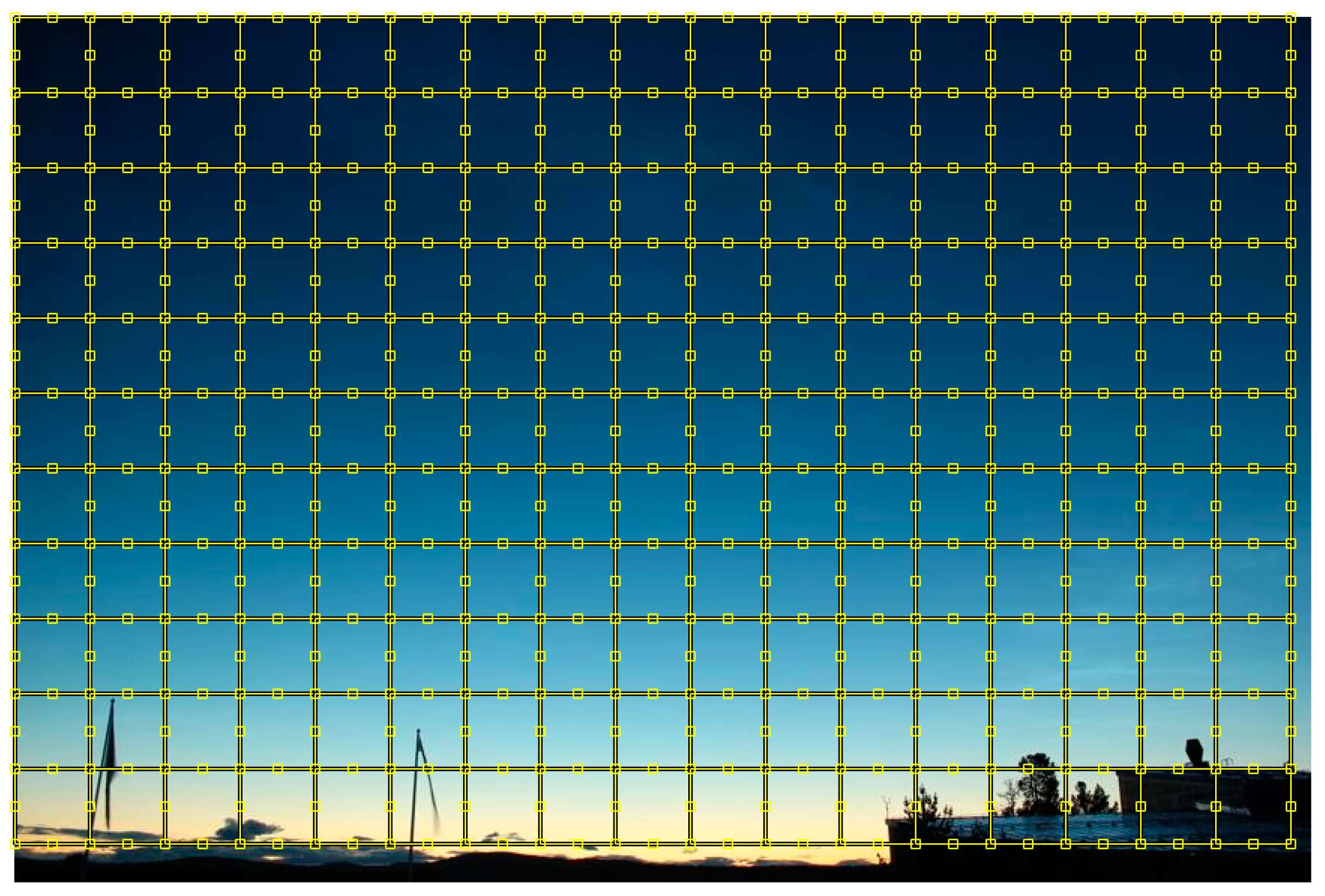
Second, as NLC activity is spatially localized in a given image, the resized image is divided into image blocks of size N-by-N pixels each as shown in
Figure 4, for our experiments we used N = 50 pixels. Image regions along the right and the bottom edges of the images are quite small in size and hence not considered. Here the choice of block size N is governed by the overall resolution of the given image. A small block size would increase the computational complexity of the analysis and can be insufficient to capture the necessary details associated with the four different classes. On the other hand, a large block size would generate a number of regions with overlapping classes which can make the discrimination challenging.
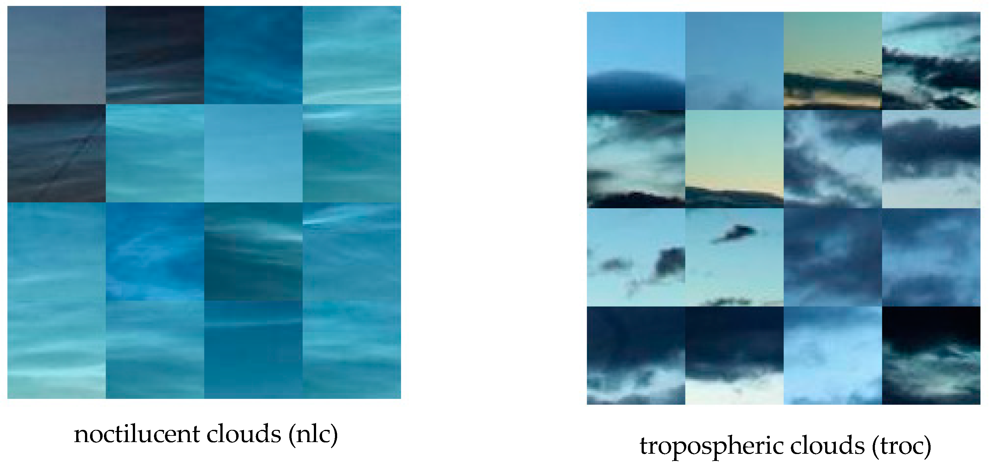
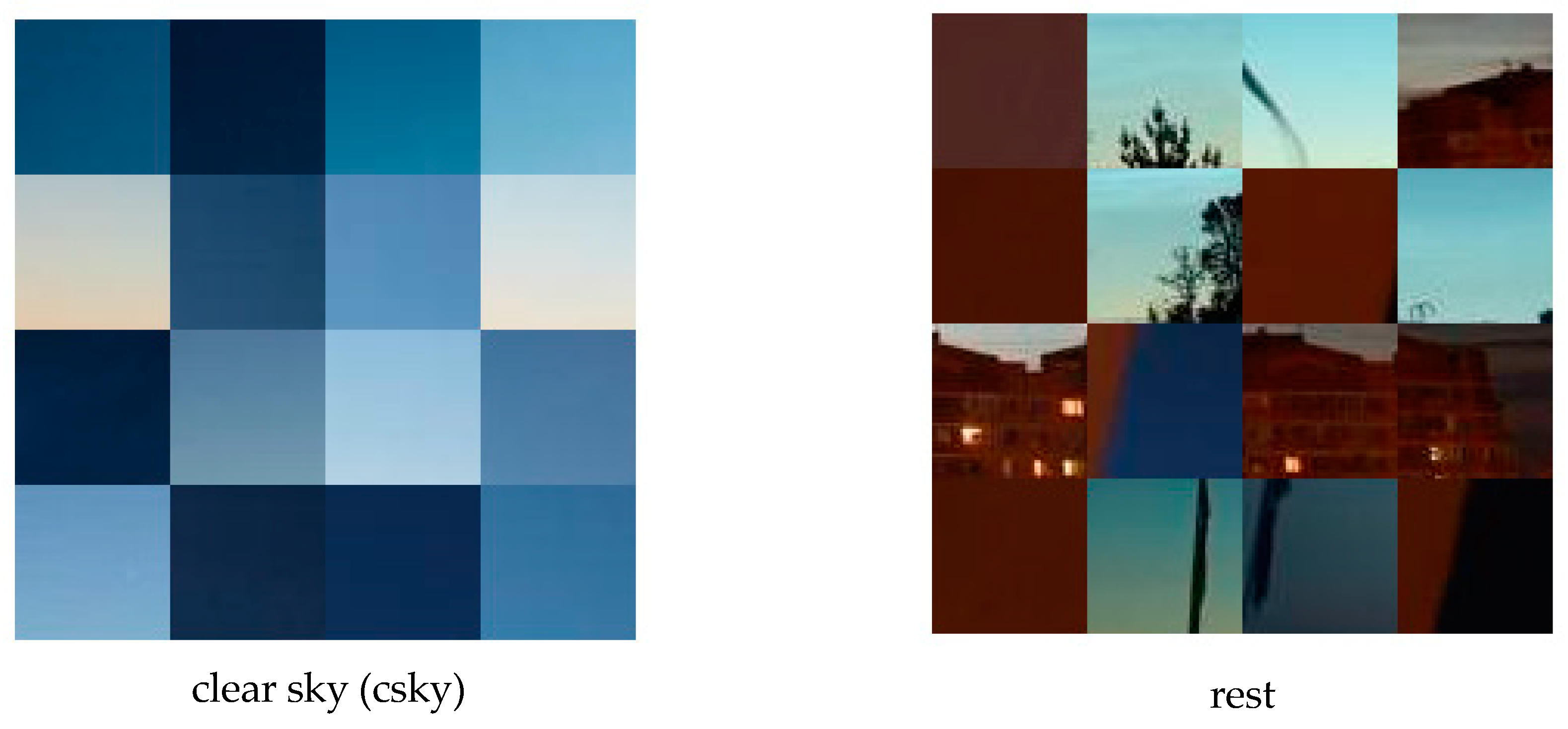
Third, image blocks from the whole dataset are divided into four different categories namely, noctilucent clouds, tropospheric clouds, clear sky, and rest that includes all objects that appear in the background of an image. A few randomly selected samples from the four categories are shown in
Figure 5. A total of 6000 samples for each category are randomly selected from the dataset. The assignment of one of the four categories to each image block is done manually. Sixty percent of the total number of samples are used for training, twenty percent are used for testing the performance of the different methods, and in case of CNN, rest twenty percent are used for validation.
3.3. Methods
3.3.1. Linear Discriminant Analysis
In literature, linear discriminant analysis (LDA) is also known as Fischer discriminant analysis [
21]. For two different classes or categories with means
and covariances
, the Fischer linear discriminant is defined as a vector
w which maximizes [
22]:
where
are the “between” and “within” class scatter matrices, and T is transpose. Here, the main idea is to reduce the dimensions by projecting the data along a vector w that preserves as much of the class discriminatory information as possible. This is achieved by estimating an optimal line w that maximizes the class means (numerator) and minimizes the class variances (denominator). LDA can also be extended to construct a discriminant function for problems with more than two classes. For details, please see [
23].
3.3.2. Feature Vectors for LDA
For LDA, we employed a range of feature vectors with simple features such as: mean (µ), standard deviation (σ), max and min, and more complex feature vectors such as: higher-order local autocorrelation and histogram of oriented gradients.
Higher-order local autocorrelation (HLAC) is a feature descriptor proposed by Otsu [
24] that can be used for image recognition. In a recent study by [
25], it has been used for object detection in satellite images. HLAC features are calculated by adding the product of intensity of a reference point
and local displacement vectors
within local neighbors [
25]. Higher-order autocorrelation is defined by
where
represents the intensity level at location
of the image. An increase in the order N also increases the number of autocorrelation functions to be computed, therefore, to enable practical use N is restricted to second-order
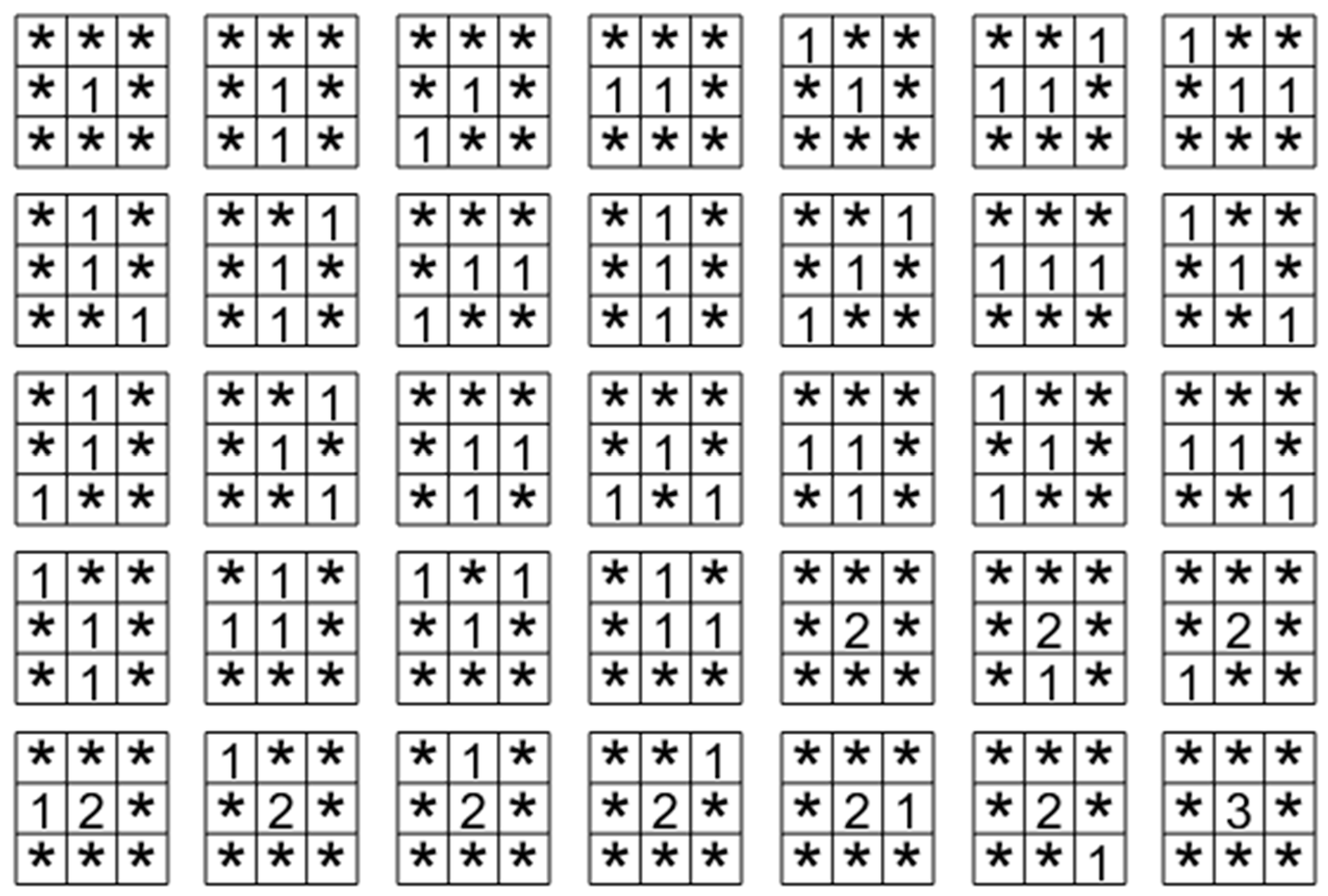
and the range of displacements is restricted to 3 by 3 with its center as the reference. There are 35 displacement masks shown in
Figure 6, and are convolved with the image and resulting values pertaining to each pattern accumulated. In each mask, the values represent the reference locations used in multiplying with the image intensities and * represents do not care locations [
25]. In this manner, a set of 35-dimensional HLAC vectors are generated from an intensity image at a given resolution. HLAC feature extraction is also performed for lower resolutions. For our calculations, we used only one resolution of the 50 by 50 pixels image block and three-color channels resulting in a feature vector of size 105.
Histogram of oriented gradients (HOG) is a feature descriptor used for object detection. The main idea behind HOG is that an object’s appearance and shape can be represented by the distribution of intensity gradients or edge directions [
26]. HOG is invariant to local geometric and photometric transformations [
26]. In the implementation of HOG [
26], first, a given image is divided into small spatial regions called cells and their gradient values are calculated. Second, for each cell, a histogram of gradient directions or edge orientations is computed. In order to account for illumination and contrast changes, the gradient values are normalized over larger spatially connected cell regions called blocks. Finally, the HOG descriptor is obtained by concatenating the components of the normalized cell histograms from all of the block regions. For our calculations, we used a cell size of 8 by 8 pixels across three RGB color channels for each input image block, resulting in a feature vector of size 2700.
3.3.3. Convolutional Neural Network
Convolutional neural network (CNN) is a class of deep neural networks commonly used for image analysis. As compared to traditional neural networks, a CNN is both computationally and statistically efficient. In part, this is due to small kernel sizes used for extracting meaningful features, which leads to fewer connections and fewer parameters to be stored in the memory [
27].
A convolutional neural network comprises an input layer, followed by multiple hidden layers, and finally an output layer. Each hidden layer usually consists of three stages [
27]. In the first stage a convolutional layer produces a set of linear activations. In the second stage, these linear activations then run through a nonlinear function such as rectified linear unit function (RELU). In the third stage, a pooling function is used to modify the output, for instance, max-pooling (MaxPool) operation selects the maximum output from the local neighborhood. As convolutional layers are fed through non-linear activation functions, it enables the entire neural network to approximate nearly any non-linear pattern [
28,
29,
30].
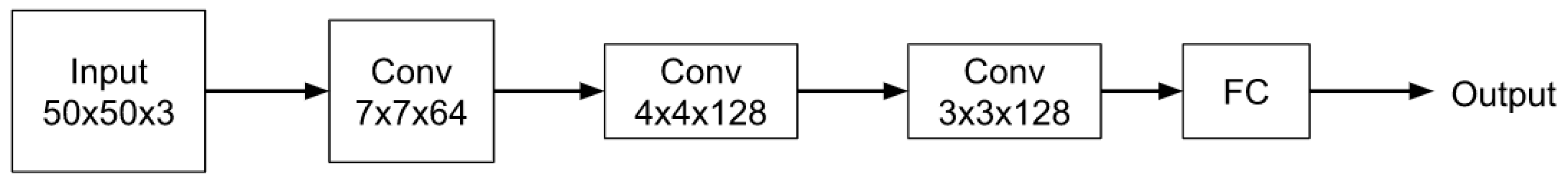
In the proposed CNN algorithm as shown in
Figure 7, the first layer allows inputs of size 50 × 50 × 3 pixels. It is followed by a three convolutional layers of size 7 × 7 × 64, 4 × 4 × 128, and 3 × 3 × 128 respectively, where the size and the number of channels for the three layers were chosen based on the performance. For details, please see
Appendix A. Each convolutional layer is followed by batch normalization, RELU, and MaxPool layer respectively. The fully connected layer is followed by a softmax layer which enables the outputs of the layer to be interpreted as probabilities and assigning a relevant class label.
4. Results
In this section, we compare the results obtained by using LDA for different feature vectors and the proposed CNN method. In the end, we visualize the performance of the CNN algorithm for a few test images.
Comparison of Different Methods
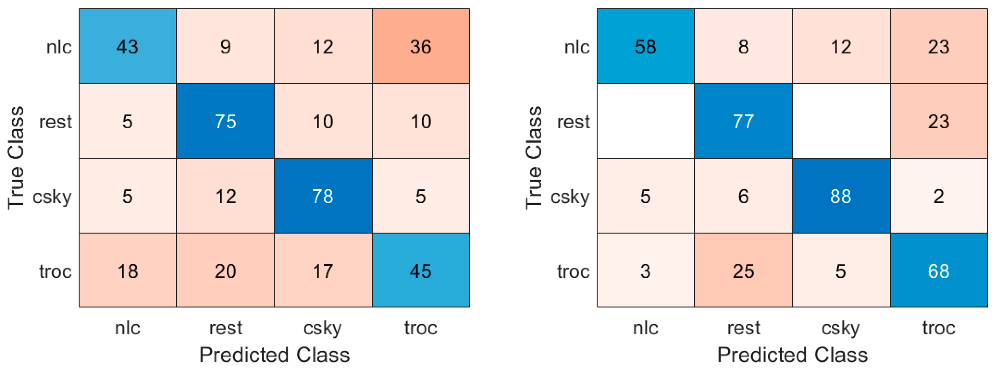
The average accuracy for the case when we use only the mean value of the image blocks for LDA is 60.19%. Here we define accuracy as the percentage of the correct number of classifications to the total number of classifications across the four different categories.
Figure 8 (left) shows the percentage of correct classifications associated with the four classes in the form of a confusion matrix. We can see that for the categories: rest and clear sky, the performances are moderate with correct classifications percentages to be 75% and 78% respectively. On the other hand, the categories: nlc and tropospheric clouds the performances are poor with correct classification percentages to be 43% and 45% respectively. When using mean and standard deviation values for LDA the average performance is improved to 72.6%, please see
Figure 8 (right). This is also visible in the four categories in
Figure 5, where the number of correct classifications improves across all four categories. However, still a significant percentage of tropospheric clouds are misclassified as rest and vice-versa, and nearly 23% of noctilucent clouds are misclassified as tropospheric clouds.
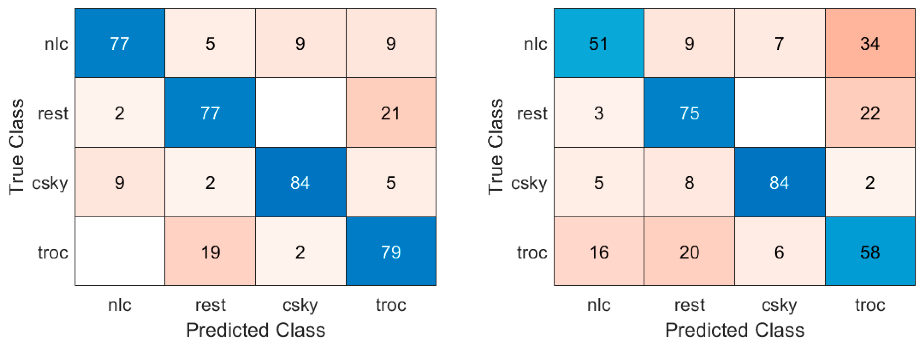
When using mean, standard deviation, minimum, and maximum values of the image regions, we observe that the performance of the discrimination across the four categories improves to 79.21%, please see
Figure 9 (left). Using HLAC as a metric for LDA decreases the average performance across the four categories to 67.08%. As shown in
Figure 9 (right), this is especially visible in the observed prediction rates of 51% and 58% for the noctilucent and tropospheric cloud classes respectively, which are affected the most.
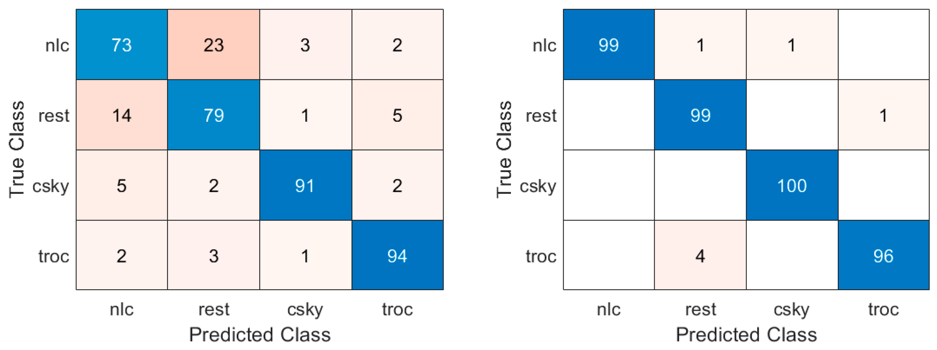
The classification scores for the four categories using HOG for LDA improve the performance to 84.27%. As shown in
Figure 10 (left), the prediction rates for clear sky and tropospheric clouds improve to 91% and 94% respectively, however, still a significant 23% of noctilucent clouds and misclassified as rest. Finally, as shown in
Figure 10 (right) the results obtained from the proposed CNN-based approach indicate good classification scores across all four categories with approximately 99% for noctilucent, 99% for rest, 100% for clear sky and 96% for tropospheric clouds.
A summary of average classification scores for the LDA method with different metrics and CNN is shown in
Table 1. We can clearly see that the CNN method with a score of 98.27% clearly outperforms the LDA-based approaches. As the proposed CNN model employs non-linear activation functions between the convolutional layers, it is able to act as an optimal classifier for the four classes of images used in this paper.
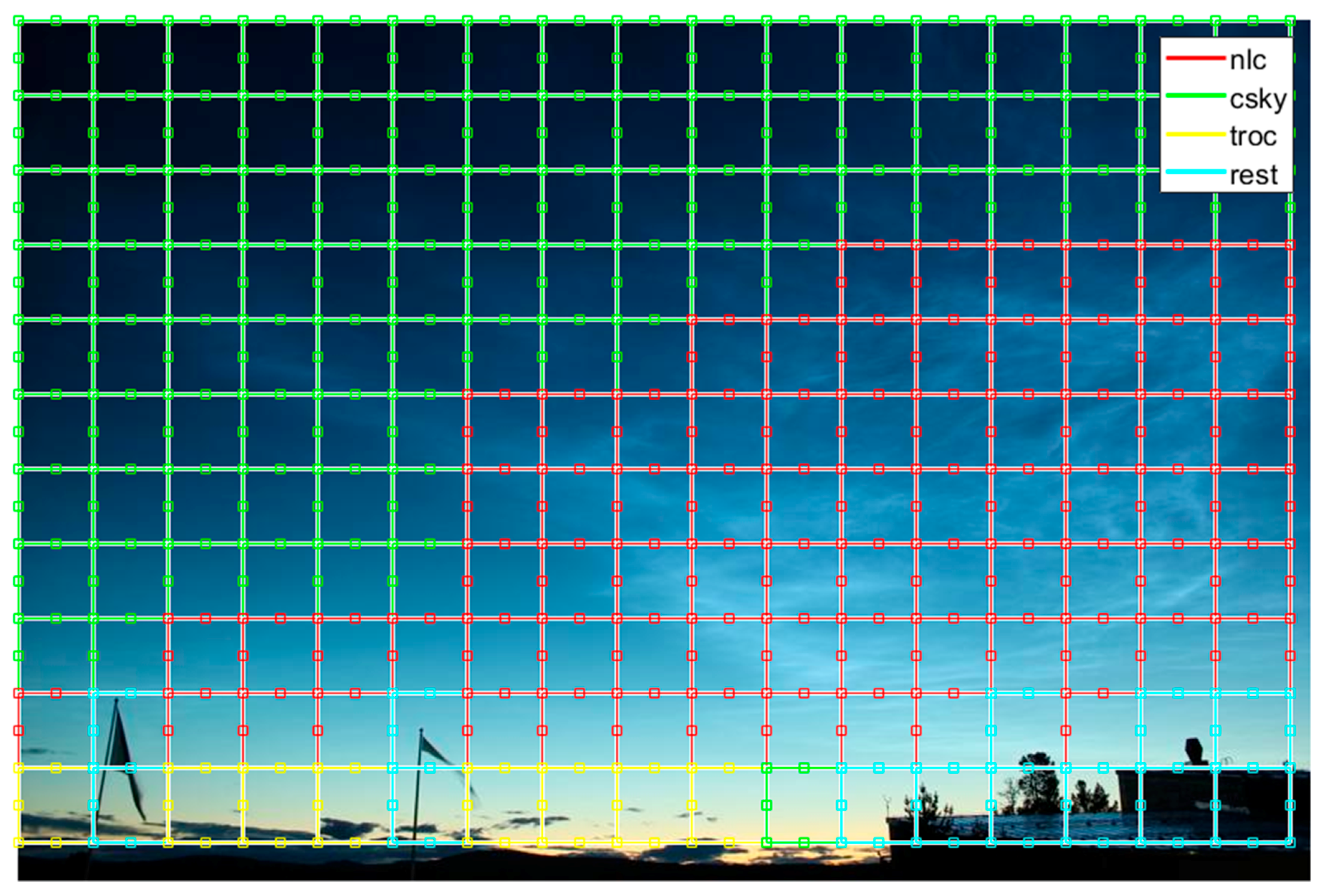
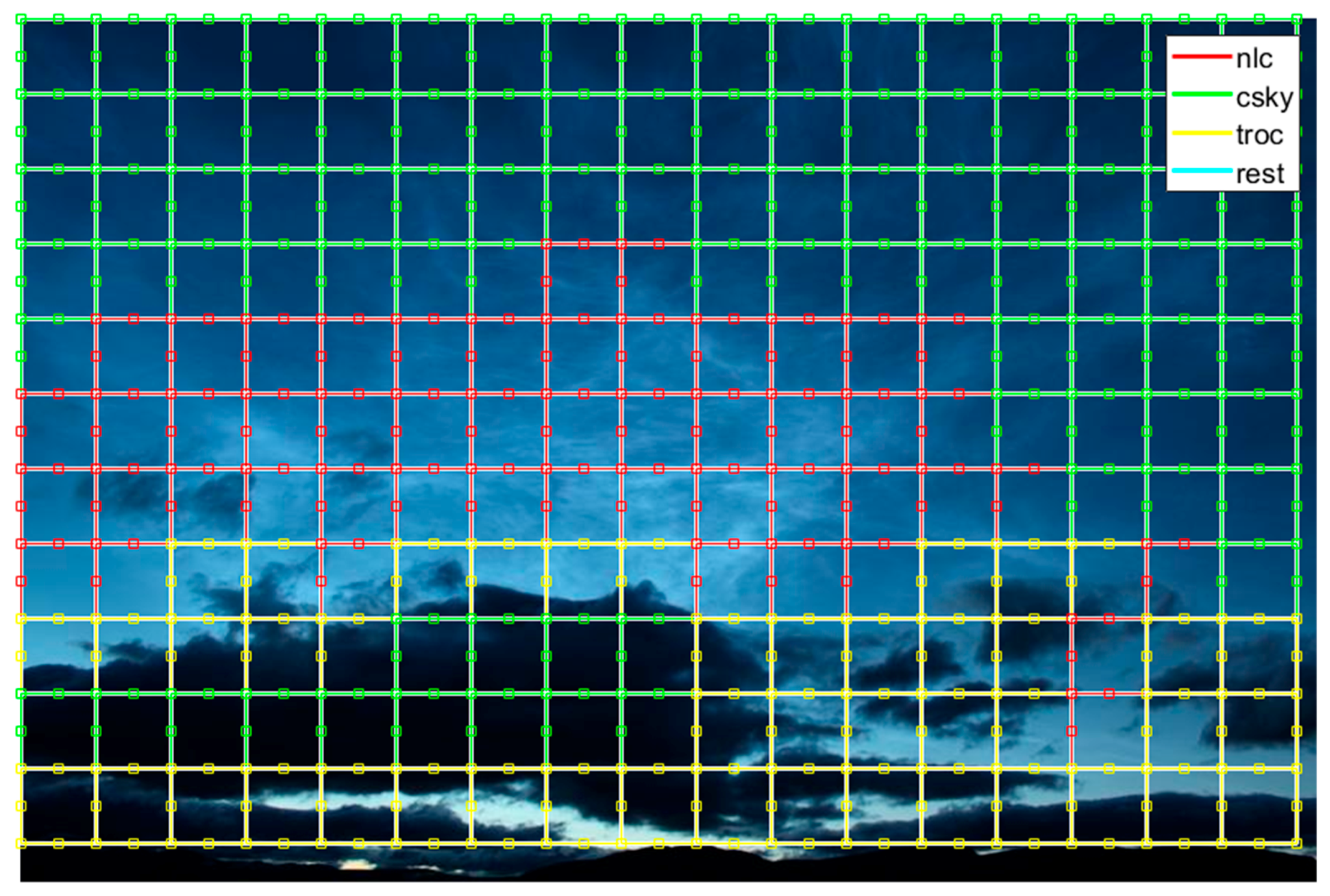
For visualization of the performance of the proposed CNN algorithm, we select five images from the three different datasets for which the CNN algorithm was not trained. As shown in
Figure 11, we can see that a majority of the noctilucent cloud activity is correctly detected by the proposed CNN algorithm. There are a few false detections in the lower left part of the image where tropospheric clouds and clear sky are predicted as noctilucent clouds. Next in
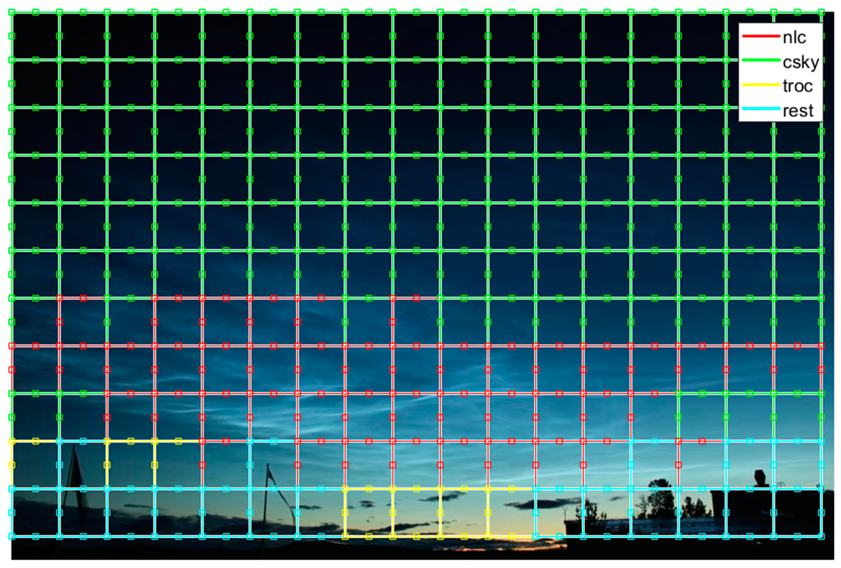
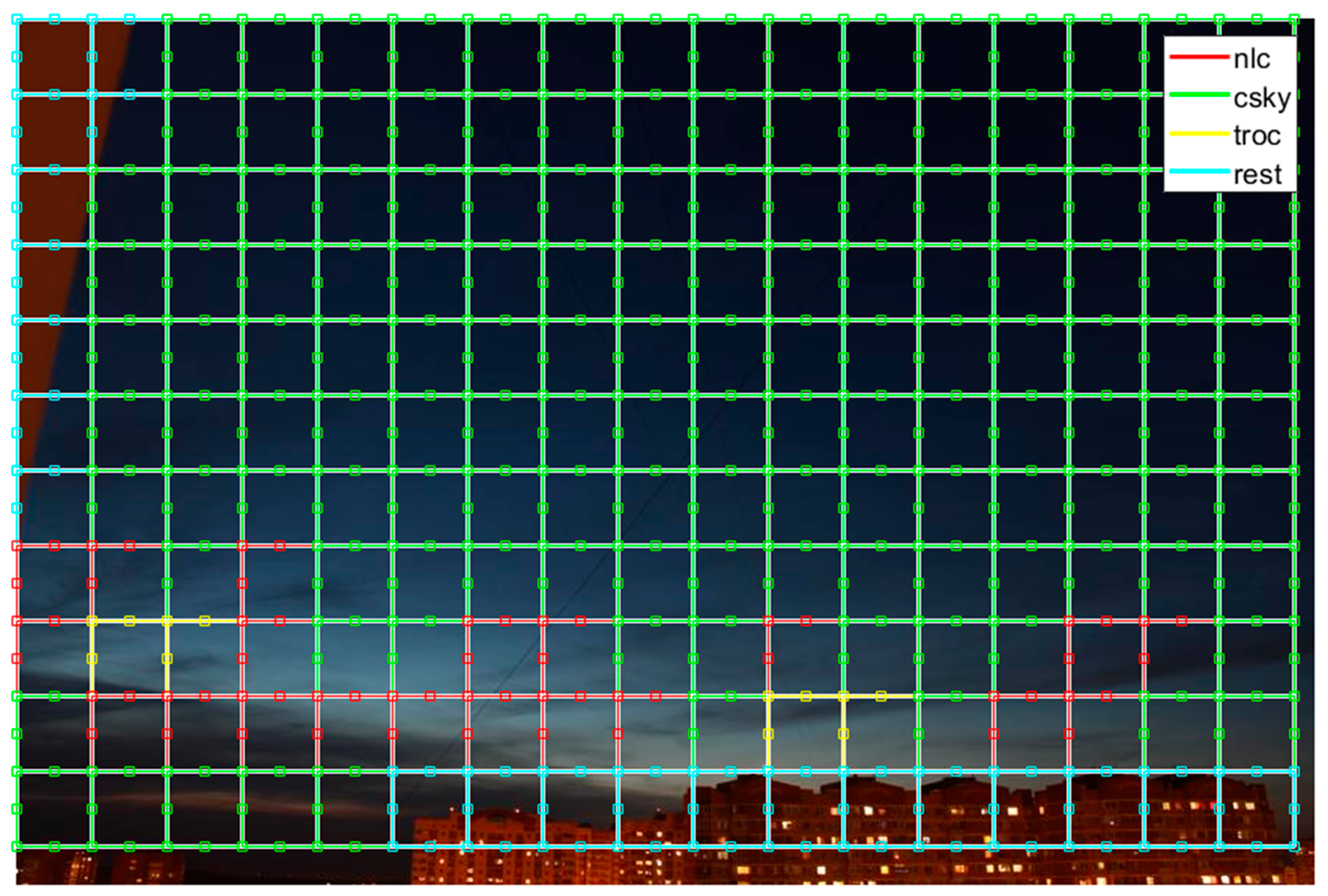
Figure 12, we can observe that a majority of the noctilucent activity including faint or low contrast noctilucent clouds are correctly predicted by the algorithm. After that in
Figure 13, we can see that very faint or low contrast activity is correctly predicted by the algorithm. Furthermore, the regions belonging to the categories such as clear sky and rest are correctly detected. In
Figure 14, we can observe a challenging scenario where noctilucent cloud activity is happening in the presence of large number of tropospheric clouds. We can see that while noctilucent cloud activity is correctly predicted, a number of tropospheric clouds regions are incorrectly classified as noctilucent clouds. Finally, in
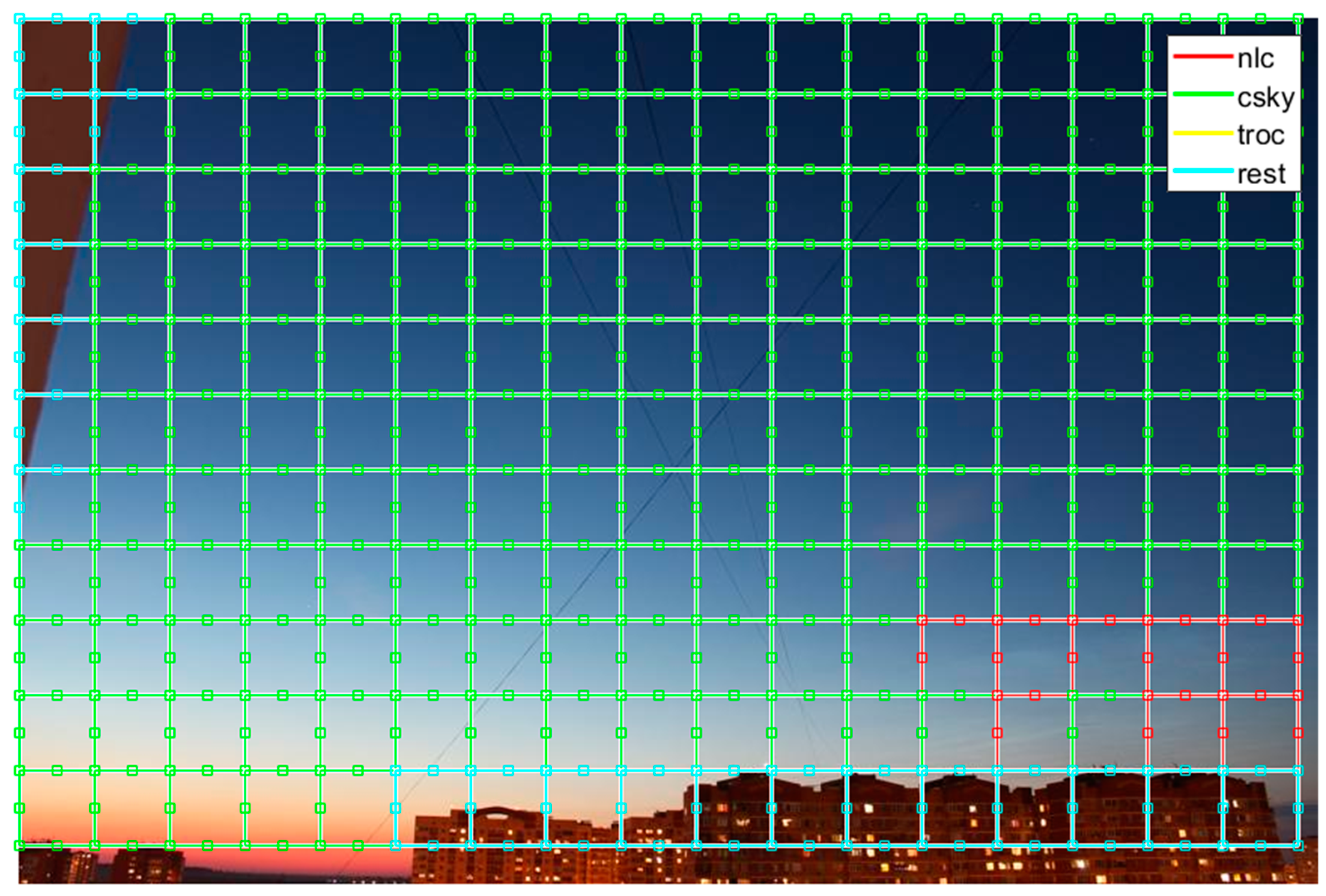
Figure 15, we present a challenging scenario which does not have any noctilucent cloud activity, here we can see that the tropospheric clouds are incorrectly predicted as noctilucent clouds. To address the issue of misclassification, we outline a few suggestions in the next section.
5. Discussion
In order to investigate if noctilucent clouds can be identified from tropospheric clouds, clear sky, and rest of the objects, first, we employed LDA. For LDA, feature vectors with simple features such as: mean, standard deviation, max and min, and more complex feature vectors such as: HLAC and HOG were used. The results from LDA show that first, LDA using mean, standard deviation, max and min values as feature vectors performs better than LDA approaches using mean only, LDA using mean and standard deviation, and LDA using HLAC. Second, LDA using HOG as feature vectors outperforms all other LDA based approaches. This implies that HOG descriptor is relatively good at capturing the features associated with noctilucent clouds that enable their discrimination from other classes. Third, as the average classification score for LDA using HOG is 84.27%, it is clear that other approaches can be used to further improve the performance of classification. For this, we propose a CNN-based method with three convolutional layers. Our results indicate that the performance of the CNN-based approach exceeds that of the LDA based approaches used in this paper. Four, a visual evaluation of the CNN algorithm for challenging cases pertaining to untested images indicates misclassifications for NLC activity.
In order to reduce the number of misclassifications associated with noctilucent cloud activity a number of possible approaches can be used: first, noctilucent clouds propagate in the mesosphere, which means that there is a temporal component linked to their start and end sequence in a scene. By employing a recurrent neural network, we can include the time component of the activity, thereby, leading to possible improvement in their prediction. As the proposed CNN algorithm would enable us to collect more data associated with noctilucent cloud activity, including the temporal component of the image sequence would be possible in future studies.
Second, to overcome the drawbacks of region-based approaches where each pixel in the region is assigned the label of the object or class in the region, a fully convolutional neural network [
31] can be employed to train and predict all the pixels associated with a scene. Fully convolutional neural networks have shown significant improvements in the state of the art pertaining to image segmentation [
31]. This approach requires a significant amount of fully labeled image data which can be mitigated by using semi-supervised learning approaches [
32]. This is something that we plan to address in the future.
6. Conclusions and Future Work
In this paper, we outline a framework to study noctilucent cloud activity for an image dataset associated with three different locations and different atmospheric conditions. For the analysis, we employ two methods: Linear discriminant analysis (LDA) with feature vectors (ranging from simple metrics to HLAC, and HOG), and convolutional neural networks (CNN). Our results imply that the CNN-based approach outperforms LDA based methods used in this paper. As a future research direction, this work can form the basis for synchronizing the optical observations from ground-based camera system with radar echoes from the EISCATincoherent scatter radar systems. While present radar observations provide limited information on the motion of the ice clouds [
10], this will be significantly improved with the new volumetric radar system EISCAT_3D [
33].
Author Contributions
P.S., P.D., and I.M. contributed to the conceptualization and methodology of the problem. P.D. provided the image data for the analysis. P.S. performed the investigation and proposed the methods used in the paper. P.S., P.D., and I.M. contributed towards the writing, editing, and review.
Funding
The publication charges for this article have been funded by a grant from the publication fund of UiT The Arctic University of Norway.
Acknowledgments
IM’s work is within a project funded by Research Council of Norway, NFR 275503. The EISCAT International Association is supported by research organizations in Norway (NFR), Sweden (VR), Finland (SA), Japan (NIPR and STEL), China (CRIPR), and the United Kingdom (NERC). EISCAT VHF and UHF data are available under
http://www.eiscat.se/madrigal/. The authors thank Andrey Reshetnikov and Alexander Dalin for their technical support of the NLC camera located in Moscow (Russia), as well as administration of Luleå University of Technology for their technical support of the NLC camera located in Kiruna (Sweden).
Conflicts of Interest
The authors declare no conflict of interest.
Appendix A
Different combinations of the size and number of channels for the three convolutional layers (shown in
Table 1) were tested. For the first convolutional layer, sizes in the range [3, 10] and a number of channels (16, 32, and 64) were tested. For the second convolutional layer, sizes in the range [3, 5] and a number of channels (32, 64, and 128) were tried. For the third, convolutional layer was fixed to a size of 3 and a number of channels (16, 32, 64, 128, and 256) were tested. The set of three convolutional layers that gave the best correct predictions is shown in
Table A1.
Table A1.
CNN algorithm layers.
Table A1.
CNN algorithm layers.
| Input Layer 50 × 50 × 3 |
|---|
| Conv 7 × 7 × 64 |
| BatchNorm |
| RELU |
| MaxPool 2 × 2 |
| Conv 4 × 4 × 128 |
| BatchNorm |
| RELU |
| MaxPool 2 × 2 |
| Conv 3 × 3 × 128 |
| BatchNorm |
| RELU |
| MaxPool 2 × 2 |
| fullyConnected |
| Softmax |
| Classification |
References
- Dalin, P.; Kirkwood, S.; Andersen, H.; Hansen, O.; Pertsev, N.; Romejko, V. Comparison of long-term Moscow and Danish NLC observations: Statistical results. Ann. Geophys. 2006, 24, 2841–2849. [Google Scholar] [CrossRef][Green Version]
- Lübken, F.-J.; Berger, U.; Baumgarten, G. On the Anthropogenic Impact on Long-Term Evolution of Noctilucent Clouds. Geophys. Res. Lett. 2018, 45, 6681–6689. [Google Scholar] [CrossRef]
- Dubietis, A.; Dalin, P.; Balčiūnas, R.; Černis, K. Observations of noctilucent clouds from Lithuania. J. Atmos. Sol. -Terr. Phys. 2010, 72, 1090–1099. [Google Scholar] [CrossRef]
- Kirkwood, S.; Dalin, P.; Réchou, A. Noctilucent clouds observed from the UK and Denmark—Trends and variations over 43 years. Ann. Geophys. 2008, 26, 1243–1254. [Google Scholar] [CrossRef]
- Pertsev, N.; Dalin, P.; Perminov, V.; Romejko, V.; Dubietis, V.; Balčiunas, R.; Černis, K.; Zalcik, M. Noctilucent clouds observed from the ground: sensitivity to mesospheric parameters and long-term time series. Earth Planets Space 2014, 66, 1–9. [Google Scholar] [CrossRef]
- Zalcik, M.; Lohvinenko, T.W.; Dalin, P.; Denig, W. North American Noctilucent Cloud Observations in 1964–77 and 1988–2014: Analysis and Comparisons. J. R. Astron. Soc. Can. 2016, 110, 8–15. [Google Scholar]
- Zalcik, M.S.; Noble, M.P.; Dalin, P.; Robinson, M.; Boyer, D.; Dzik, Z.; Heyhurst, M.; Kunnunpuram, J.G.; Mayo, K.; Toering, G.; et al. In Search of Trends in Noctilucent Cloud Incidence from the La Ronge Flight Service Station (55N 105W). J. R. Astron. Soc. Can 2014, 108, 148–155. [Google Scholar]
- Russell, J.M., III; Rong, P.; Hervig, M.E.; Siskind, D.E.; Stevens, M.H.; Bailey, S.M.; Gumbel, J. Analysis of northern midlatitude noctilucent cloud occurrences using satellite data and modeling. J. Geophys. Res. Atmos. 2014, 119, 3238–3250. [Google Scholar] [CrossRef]
- Hervig, M.E.; Berger, U.; Siskind, D.E. Decadal variability in PMCs and implications for changing temperature and water vapor in the upper mesosphere. J. Geophys. Res. Atmos. 2016, 121, 2383–2392. [Google Scholar] [CrossRef]
- Mann, I.; Häggström, I.; Tjulin, A.; Rostami, S. First wind shear observation in PMSE with the tristatic EISCAT VHF radar. J. Geophys. Res. Space Phys. 2016, 121, 11271–11281. [Google Scholar] [CrossRef]
- Fritts, C.D.; Alexander, M.J. Gravity wave dynamics and effects in the middle atmosphere. Rev. Geophys. 2003, 41, 1–64. [Google Scholar] [CrossRef]
- Lübken, F.-J. Thermal structure of the Arctic summer mesosphere. J. Geophys. Res. Atmos. 1999, 104, 9135–9149. [Google Scholar]
- Nussbaumer, V.; Fricke, K.H.; Langer, M.; Singer, W.; von Zahn, U. First simultaneous and common volume observations of noctilucent clouds and polar mesosphere summer echoes by lidar and radar. J. Geophys. Res. Atmos. 1996, 101, 19161–19167. [Google Scholar] [CrossRef]
- Rapp, M.; Lübken, F.J. Polar mesosphere summer echoes (PMSE): Review of observations and current understanding. Atmos. Chem. Phys. 2004, 4, 2601–2633. [Google Scholar] [CrossRef]
- Schwartz, M.J.; Lambert, A.; Manney, G.L.; Read, W.G.; Livesey, N.J.; Froidevaux, L.; Ao, C.O.; Bernath, P.F.; Boone, C.D.; Cofield, R.E.; et al. Validation of the Aura Microwave Limb Sounder temperature and geopotential height measurements. J. Geophys. Res. Atmos. 2008, 113. [Google Scholar] [CrossRef]
- Froidevaux, L.; Livesey, N.J.; Read, W.G.; Jiang, Y.B.; Jimenez, C.; Filipiak, M.J.; Schwartz, M.J.; Santee, M.L.; Pumphrey, H.C.; Jiang, J.H.; et al. Early validation analyses of atmospheric profiles from EOS MLS on the aura Satellite. IEEE Trans. Geosci. Remote Sens. 2006, 44, 1106–1121. [Google Scholar] [CrossRef]
- Gadsden, M.; Schröder, W. Noctilucent Clouds (Physics and Chemistry in Space), 1st ed.; Springer: Berlin/Heidelberg, Germany, 1989; Volume IX, p. 165. [Google Scholar]
- Mann, I.; Gunnarsdottir, T.; Häggström, I.; Eren, S.; Tjulin, A.; Myrvang, M.; Rietveld, M.; Dalin, P.; Jozwicki, D.; Trollvik, H. Radar studies of ionospheric dusty plasma phenomena. Contrib. Plasma Phys. 2019, 59, e201900005. [Google Scholar] [CrossRef]
- Association, E.S. EISCAT European Incoherent Scatter Scientific Association Annual Report 2011; EISCAT Scientific Association: Kiruna, Sweden, 2011. [Google Scholar]
- Leyser, B.T.; Wong, A.Y. Powerful electromagnetic waves for active environmental research in geospace. Rev. Geophys. 2009, 47. [Google Scholar] [CrossRef]
- Theodoridis, S.; Koutroumbas, K. Pattern Recognition, 4th ed.; Academic Press: Cambridge, MA, USA, 2008; p. 984. [Google Scholar]
- Mika, S.; Ratsch, G.; Weston, J.; Scholkopf, B.; Mullers, K.R. Fisher discriminant analysis with kernels. In Proceedings of the Neural Networks for Signal Processing IX: Proceedings of the 1999 IEEE Signal Processing Society Workshop (Cat. No.98TH8468), Madison, WI, USA, 25 August 1999; IEEE: Piscataway, NJ, USA, 1999. [Google Scholar]
- Rao, C.R. The Utilization of Multiple Measurements in Problems of Biological Classification. J. R. Stat. Soc. 1948, 10, 159–203. [Google Scholar] [CrossRef]
- Nomoto, N.; Shinohara, Y.; Shiraki, T.; Kobayashi, T.; Otsu, N. A New Scheme for Image Recognition Using Higher-Order Local Autocorrelation and Factor Analysis. In Proceedings of the MVA2005 IAPR Conference on Machine Vision Applications, Tsukuba, Japan, 16–18 May 2005; pp. 265–268. [Google Scholar]
- Uehara, K.; Sakanashi, H.; Nosato, H.; Murakawa, M.; Miyamoto, H.; Nakamura, R. Object detection of satellite images using multi-channel higher-order local autocorrelation. In Proceedings of the IEEE International Conference on Systems, Man, and Cybernetics (SMC), Banff, AB, Canada, 5–8 October 2017; IEEE: Piscataway, NJ, USA, 2017; pp. 1339–1344. [Google Scholar]
- Dalal, N.; Triggs, B. Histograms of oriented gradients for human detection. In Proceedings of the 2005 IEEE Computer Society Conference on Computer Vision and Pattern Recognition (CVPR’05), San Diego, CA, USA, 20–26 June 2017; pp. 886–893. [Google Scholar]
- Goodfellow, I.; Bengio, Y.; Courville, A. Deep Learning; MIT Press: Cambridge, MA, USA, 2016. [Google Scholar]
- Sonoda, S.; Murata, N. Neural network with unbounded activation functions is universal approximator. Appl. Comput. Harmon. Anal. 2017, 43, 233–268. [Google Scholar] [CrossRef]
- Lundervold, S.A.; Lundervold, A. An overview of deep learning in medical imaging focusing on MRI. Z. Med. Phys. 2019, 29, 102–127. [Google Scholar] [CrossRef] [PubMed]
- Leshno, M.; Lin, V.Y.; Pinkus, A.; Schocken, S. Multilayer feedforward networks with a nonpolynomial activation function can approximate any function. Neural Netw. 1993, 6, 861–867. [Google Scholar] [CrossRef]
- Long, J.; Shelhamer, E.; Darrell, T. Fully convolutional networks for semantic segmentation. In Proceedings of the 2015 IEEE Conference on Computer Vision and Pattern Recognition (CVPR), Boston, MA, USA, 7–12 June 2015. [Google Scholar]
- Enguehard, J.; O’Halloran, P.; Gholipour, A. Semi-Supervised Learning With Deep Embedded Clustering for Image Classification and Segmentation. IEEE Access 2019, 7, 11093–11104. [Google Scholar] [CrossRef] [PubMed]
- Wannberg, U.G.; Eliasson, L.; Johansson, J.; Wolf, I.; Andersson, H.; Bergqvist, P.; Bergqvist, P.; Häggström, I.; Iinatti, T.; Laakso, T.; et al. Eiscat_3d: A next-generation European radar system for upper-atmosphere and geospace research. Ursi Radio Sci. Bull. 2010, 2010, 75–88. [Google Scholar]
© 2019 by the authors. Licensee MDPI, Basel, Switzerland. This article is an open access article distributed under the terms and conditions of the Creative Commons Attribution (CC BY) license (http://creativecommons.org/licenses/by/4.0/).


