ASTER Cloud Coverage Assessment and Mission Operations Analysis Using Terra/MODIS Cloud Mask Products


1
Department of Computer and Information Sciences, Ibaraki University, Hitachi, Ibaraki 3168511, Japan
2
Japan Space Systems, Minato-ku, Tokyo 1050011, Japan
*
Author to whom correspondence should be addressed.
Remote Sens. 2019, 11(23), 2798; https://doi.org/10.3390/rs11232798
Submission received: 29 September 2019
/
Revised: 22 November 2019
/
Accepted: 23 November 2019
/
Published: 26 November 2019
(This article belongs to the Special Issue ASTER 20th Anniversary)
Abstract
:Since the Advanced Spaceborne Thermal Emission and Reflection Radiometer (ASTER) instrument cannot detect clouds accurately for snow-covered or nighttime images due to a lack of spectral bands, Terra/MODIS cloud mask (MOD35) products have been alternatively used in cloud assessment for all ASTER images. In this study, we evaluated ASTER cloud mask images generated from MOD35 products and used them to analyze the mission operations of ASTER. In the evaluation, ASTER cloud mask images from different MOD35 versions (Collections 5, 6, and 6.1) showed a large discrepancy in low- or high-latitude areas, and the rate of ASTER scenes with a high uncertain-pixel rate (≥30%) showed to be 2.2% in daytime and 12.0% in nighttime. In the visual evaluation with ASTER browse images, about 2% of cloud mask images showed some problems such as mislabeling and artifacts. In the mission operations analysis, the cloud avoidance function implemented in the ASTER observation scheduler showed a decrease in the mean cloud coverage (MCC) and an increase in the rate of clear scenes by 10% to 15% in each. Although 19-year-old time-series of MCC in five areas showed weather-related fluctuations such as the El Niño Southern Oscillation (ENSO), they indicated a small percent reduction in MCC by enhancement of the cloud avoidance function in April 2012. The global means of the number of clear ASTER scenes were 15.7 and 6.6 scenes in daytime and nighttime, respectively, and those of the success rate were 33.3% and 40.4% in daytime and nighttime, respectively. These results are expected to contribute not only to the ASTER Project but also to other optical sensor projects.
1. Introduction
The Advanced Spaceborne Thermal Emission and Reflection Radiometer (ASTER) is an optical sensor onboard NASA’s Terra satellite launched on 18 December 1999 [1]. The ASTER instrument has 14 spectral bands divided by the following three subsystems: the visible and near-infrared (VNIR) subsystem (three bands), the shortwave infrared (SWIR) subsystem (six bands), and the thermal infrared (TIR) subsystem (five bands). The spatial resolution is 15 m, 30 m, and 90 m, for the VNIR, the SWIR, and the TIR subsystems, respectively, and the swath width of each subsystem is 60 km. Table 1 gives the spectral range and the ground resolution of each ASTER band [1]. ASTER products have been widely used in various fields such as surface mineralogical mapping, long-term global monitoring of glaciers, volcanoes, and coral reefs, as well as regional surface heat balance analysis [2].
In the generation of such products, cloud coverage (CC) assessment for each scene is a fundamental procedure. An assessment result is used not only for higher product generation but also for purposes such as image search and mission operations analysis. In the ASTER level-1 processing, the ASTER cloud cover assessment algorithm (ACCAA) has been implemented [3,4]. The original ACCAA which is a modified version of the automatic cloud cover assessment (ACCA) of Landsat-5 TM [5] uses three filters (i.e., threshold tests) with ASTER bands 2 (VNIR), 4 (SWIR), and 11 (TIR). Since 28 October 2000, an improved version of ACCAA has been used for all ASTER scenes observed in the full mode in which all bands are on [6]. This improved version which was developed based on the ACCA of Landsat-7 ETM+ [5] has eight filters with bands 1 to 3 (VNIR), band 4 (SWIR) and band 13 (TIR) and two passes, where the pass one goal is to develop a reliable cloud signature for use in pass two where the remaining clouds are identified [5]. The improved ACCAA is more accurate than the original ACCAA, but it performs less well in some combinations of surface type and sun elevation angle such as desert observation under a low sun elevation [6]. In addition, the original and the improved ACCAAs are not accurate enough for nighttime scenes due to thresholding with single TIR band [7], and also became unreliable particularly in the cryosphere after April 2008, because SWIR imaging has been saturated due to anomalously high SWIR detector temperature [8]. Although Hulley and Hook have proposed a new methodology for ASTER cloud detection and classification [9], on the one hand, it is difficult to use in operation due to a lack of SWIR bands. On the other hand, the Moderate Resolution Imaging Spectroradiometer (MODIS) onboard the Terra satellite provides cloud mask (MOD35) products [10,11] by simultaneous observations with ASTER using effective bands for cloud detection, although the spatial resolution is lower than ASTER. Thus, the ASTER Project has operated the ASTER CC reassessment system using MOD35 products since June 2009 [6,12]. In this system, ASTER cloud mask images are generated from only collocated MOD35 products and used for recalculation of ASTER CC values. ASTER cloud mask images generated are provided to the public through the Internet [13].
Thus, in this study, we evaluate the reliability of MOD35-based ASTER cloud mask images, and, then, perform ASTER mission operations analysis using those cloud mask images. As for the accuracy of MOD35 products, Ackerman et al. performed a comprehensive study for Collection 5 (C5) MOD35 products using lidar data [14], and Wilson et al. reported that C5 MOD35 products have a bias induced by land cover types [15]. Wang et al. evaluated C6 Aqua/MODIS cloud mask (MYD35) products using Cloud-Aerosol Lidar and Infrared Pathfinder Satellite Observations (CALIPSO) products [16], and Moeller et al. described improvements of MOD35 products in updating from C6 to C6.1 [17]. These studies, however, do not focus on usage of MOD35 products in cloud assessment for a type of high-resolution sensor such as ASTER. For the evaluation of the reliability of MOD35-based ASTER cloud mask images, we, therefore, report results for a comparison among C5, C6, and C6.1 MOD35 products, an evaluation of uncertain pixels in MOD35 products, and a visual evaluation with ASTER browse images. Although the visual evaluation of MOD35-based ASTER cloud masks was reported by Tonooka et al. [6], we demonstrate an updated result using C6.1 MOD35 products as of August 2019.
With respect to ASTER mission operations analysis using cloud mask images, we report results of an effectiveness evaluation of the cloud avoidance function implemented in the ASTER observation scheduler [18]. The cloud avoidance function of the ASTER scheduler has not been evaluated in the past. We also report results from the time-series analysis of the mean cloud coverage, and from global mapping of the number of clear scenes and the success rate, where, in this study, the success rate is defined as the rate of clear scenes with a CC of 20% or less. Although King et al. reported the global maps of the seasonal mean cloud fraction using MODIS C5.1 cloud products from 2000 to 2011 [19], our time-series analysis and global mapping with MOD35 products differs from their study in that we use only MOD35 products accompanied by ASTER observations mainly over land areas. Since Tonooka et al. have already performed global mapping of a number of clear scenes and the success rate for ASTER using C5 MOD35 products as of 2010 [6], we demonstrate updated results using C6.1 MOD35 products as of August 2019.
2. Materials and Methods
2.1. ASTER Cloud Coverage Reassessment Using MOD35 Products
2.1.1. Overview of MOD35 Products
The MOD35 product is a level-2 product with a spatial resolution of 1 km or 250 m [10,11]. In the ASTER Project, the MOD35 product with a spatial resolution of 1 km is used for CC reassessment, because a spatial resolution of 250 m is not available in nighttime [6]. In the MOD35 algorithm, each pixel is classified to a particular domain according to surface type and solar illumination, and then tested by a series of threshold tests prepared for each domain. According to the confidence flag calculated through these tests, one of four levels (0, cloudy; 1, uncertain; 2, probably clear; and 3, clear) is assigned to each pixel as a cloud mask value. The details on this algorithm can be found in [10,11].
The MOD35 algorithm was significantly improved in C4 to C5 updating, particularly for polar regions and oceans in nighttime [20]. Ackerman et al. validated C5 MOD35 products through lidar observations from ground, aircraft, and spaceborne platforms, concluding that the MODIS algorithm agreed with the lidar about 85% of the time, the optical depth limitation of the MODIS cloud mask was approximately 0.4, and approximately 90% of the mislabeled scenes had optical depths less than 0.4 [14]. Wilson et al. pointed out that C5 MOD35 cloud mask had a systematic land cover bias, and this bias partly remained also in C6 MOD35 cloud mask [15].
In updating from C5 to C6, various improvements such as use of normalized difference vegetation index (NDVI) background maps and addition of a new night ocean test were applied [11,21]. Wang et al. evaluated C6 MYD35 products using Cloudsat CALIPSO products, showing that the total agreement (the sum of the clear- and cloud-hit rates) between them was 77.8%, and MODIS mislabeled cloud as clear for 9.1% and clear as cloudy for 1.8% [16].
2.1.2. ASTER Cloud Coverage Reassessment System
The ASTER CC reassessment system generates a cloud mask image of each ASTER scene from the MOD35 product simultaneously observed with ASTER, and calculates the CC of that ASTER scene [6]. The system has been operated by Ibaraki University since June 2009, now providing a reassessment result in two days after each ASTER observation. The system has the following procedures:
- Obtain daily ASTER catalogue information from Japan Space Systems (JSS);
- Obtain MOD35 products from NASA Goddard Space Flight Center (GSFC);
- Generate cloud mask images for all ASTER scenes in the catalogue;
- Send the reassessment results (CC etc.) to JSS, Land Processes Distributed Active Archive Center (LP DAAC), and Institute of Advanced Industrial Science and Technology (AIST);
- Release ASTER cloud mask images to public through Internet [13].
The cloud mask for each scene has the same size with an ASTER/TIR level-1A image (700 × 700 pixels) by assignment of MOD35 results to ASTER/TIR pixels with the nearest neighbor interpolation. The CC of each ASTER scene is calculated from each cloud mask by giving 100% to cloud pixels, 50% to uncertain pixels, and 0% to probably clear or clear pixels, and averaging them over the scene. Since the rate of uncertain pixels in each scene can be used as a reliability index, this value is added as an ancillary information to the delivered result.
Although the system started with C5 MOD35 products, C6.1 MOD35 products have being used since January 2017. Reprocessing with C6.1 MOD35 products was completed for all ASTER archives.
As of 10 August 2019, the total number of ASTER scenes accompanied with MOD35-based cloud masks is 3,618,286, 99.4% of all ASTER archives (equals 3,640,027). The rate of ASTER scenes without MOD35-based cloud masks is 0.71% in daytime observations, and 0.23% in nighttime observations. The reason why daytime observations have more losses is because Terra MODIS had more observation losses in the period of 2000 to 2001 in which ASTER did not have many observations in nighttime. Main causes of MODIS observation losses which affected ASTER cloud reassessment are events such as Solid State Recorder (SSR) anomaly, Science Formatting Equipment (SFE) anomaly, and Terra’s maneuver [24].
2.2. Evaluation of MOD35-Based ASTER Cloud Masks
2.2.1. Comparison of ASTER Cloud Coverage Among MOD35 Versions
In the ASTER CC reassessment system, three versions of MOD35 products, C5, C6, and C6.1, have been used since June 2009. Since the CC values based on C5 or C6 MOD35 products were distributed to ASTER users before January 2018, we randomly selected 17,845 daytime scenes and 8521 nighttime scenes from ASTER scenes observed in 2016 (13.3% and 14.2% of daytime and nighttime scenes in 2016, respectively), and compared the CC values among C5, C6, and C6.1. The results are described in Section 3.1.1.
2.2.2. Rate of High-Uncertain Scenes
Since a MOD35 product with many pixels labeled as “uncertain” will be less reliable, the rate of uncertain pixels in an ASTER cloud mask image can be used as an index of reliability for that cloud mask image. We, therefore, mapped the rate of high-uncertain scenes (referred to as the high-uncertain rate) over 0.1 × 0.1 degree grids for daytime and nighttime using all ASTER archives as of 10 August 2019, where a high-uncertain scene is defined as a scene that the rate of uncertain pixels in that scene is 30% or greater. The results can be found in Section 3.1.2.
2.2.3. Visual Evaluation of ASTER Cloud Mask Images Using Browse Images
C5-based ASTER cloud mask images have been visually evaluated with ASTER browse images by human analysts [6]. In this study, we evaluated C6.1-based ASTER cloud mask images in the same way, although this approach is affected by ambiguity in human judgment.
First, we selected daytime and nighttime scenes randomly from all ASTER archives, and acquired the VNIR, SWIR, and TIR browse images for each daytime scene, and the TIR browse image for each nighttime scene. Then, we visually evaluated consistency between the C6.1-based ASTER cloud mask image and the browse image(s) for each of evaluable scenes in the selected scenes. The total number of evaluated scenes is 24,706 for daytime, and 8006 for nighttime, corresponding to about 0.9% and 1.0% of all daytime and nighttime scenes, respectively. The results are described in Section 3.1.3.
2.3. ASTER Mission Operations Analysis Using MOD35-Based ASTER Cloud Masks
2.3.1. Validation of the Cloud Avoidance Function in the ASTER Observation Scheduler
The ASTER instrument has the pointing function because the swath width of 60 km is narrower than the orbit-to-orbit distance at the equator (172 km) [1]. Using this function effectively, on the one hand, ASTER needs to respond to various observation requests such as global mapping, scientific studies, disaster monitoring, and calibration. On the other hand, the ASTER instrument has a limited duty cycle of 8%, corresponding to the two-orbit maximum data acquisition time of 16 min, mainly due to limitations in the data volume allocated in Terra’s SSR, and the communications link with the Tracking and Data Relay Satellite System (TDRSS) and ground stations [1,18]. In addition, ASTER has several instrumental limitations such as the operating time and the total number of pointing changes. Thus, the ASTER Project has developed and used the ASTER observation scheduler for responding to many observation requests optimally under various limitations throughout the mission period [18].
Basically, an observation schedule is generated on a day-by-day basis using the ASTER observation scheduler. This is called a one-day schedule (ODS). Each ODS is generated as of two or more days before each observation day. This is called a normal ODS (referred to as N-ODS in this paper). Each ODS is regenerated as of 16 hours before each observation time, and each N-ODS is replaced by that. This is called a late-change ODS (referred to as LC-ODS in this paper). In generation of N-ODS and LC-ODS, the priority function for each observation request is first calculated by multiplying eleven subfunctions from f1 to f11. Next, the score of each observation request is calculated by multiplying the priority function of that request with the overlapping area of the requested and the overpassed areas. The derived score is then compared among conflicting requests, and the observation request with the maximum score is finally selected and included in ODS. In this procedure, various instrumental limitations are also considered.
In the eleven subfunctions, f4 is the subfunction prepared for avoiding clouds and increasing cloud-free scenes. This subfunction is calculated by
where Cmax is the maximum CC accepted by each observation request; Cpred is the predicted CC for each observation request; and a, b, and κ are fixed coefficients. Although the values of a and b have not been changed since the launch (a = 1 and b = 1.5708), the value of κ was changed from 50 to 10,000,000 in April 2012 for enhancing the effect of the cloud avoidance function. Using the updated value of κ, the value of f4 is about 10−5.4 for Cmax < Cpred, and about 10+0.6 for Cmax > Cpred. A notable point here is that f4 is calculated for LC-ODS, but not for N-ODS, because the cloud prediction is generally less accurate as of two days before each observation day. Thus, a cloud prediction result is used in only LC-ODS, where the cloud prediction dataset used for LC-ODS is the total cloud coverage (TCC) which is the “TCDC: entire atmosphere” layer extracted from the “T1534 Semi-Lagrangian grid” data produced by the Global Forecast System (GFS) of National Centers for Environmental Prediction (NCEP) [25]. TCC provides a 6 h averaged CC with the horizontal resolution of 3072 E-W grids and 1536 N-S grids at 6 h intervals until 72 hours after the present.
f4 = b + a × arctan{ κ × (1 − Cmax) × (Cmax − Cpred)},
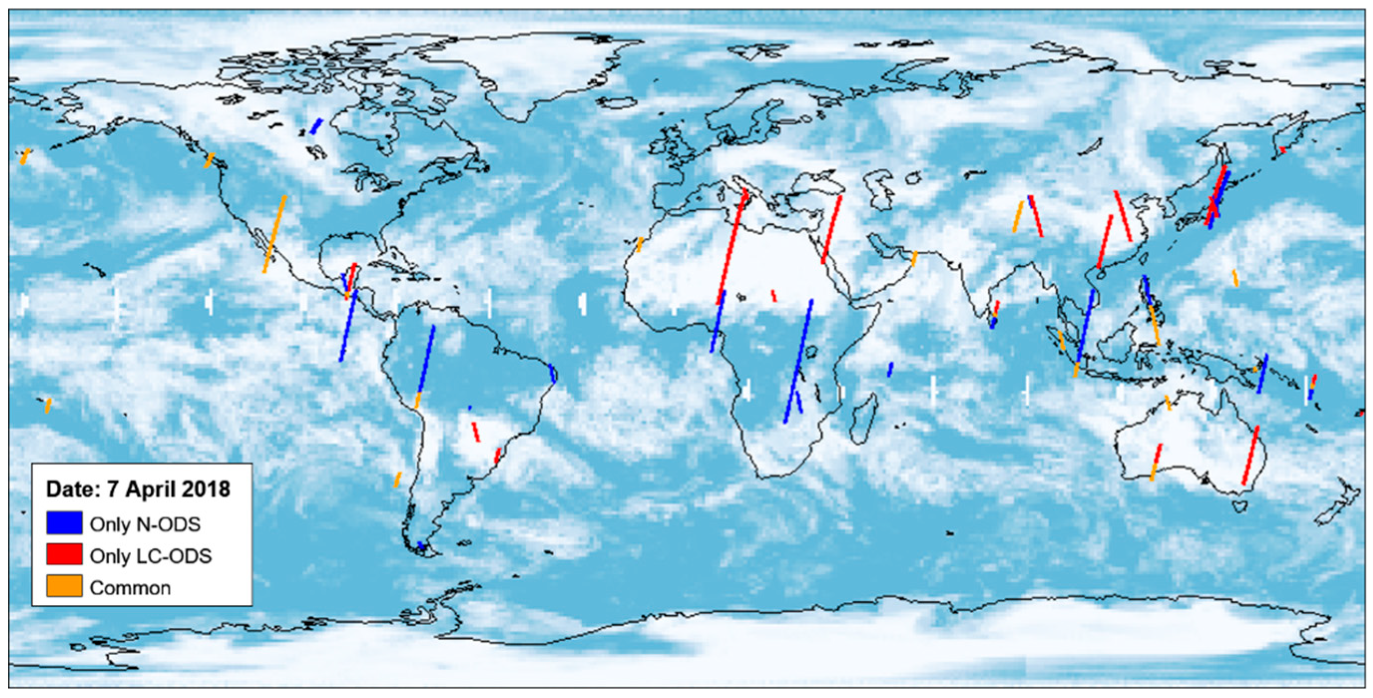
As an example, Figure 1 shows observation areas scheduled on 7 April 2018, where the background is the daily cloud fraction image from the MODIS MOD08 product on the same day. “Only N-ODS” and “only LC-ODS” show scheduled areas included in only N-ODS and in only LC-ODS, respectively, and “Common” shows scheduled areas included in both N-ODS and LC-ODS. The common scenes of N-ODS and LC-ODS account for about a half of the total scenes of LC-ODS on average. Figure 1 indicates that the cloud avoidance function worked well as expected, but it should be more quantitatively evaluated by a comparison of CC between actually observed ASTER scenes included in only LC-ODS and not-observed (fictitious) ASTER scenes included in only N-ODS on a day-by-day basis. Although fictitious ASTER scenes do not exist, the CCs of them can be calculated by a combination of N-ODS data and MOD35 products. Thus, we evaluated the effectiveness of the cloud avoidance function in the ASTER observation scheduler by this approach using the ASTER cloud reassessment system.
First, we investigated which areas were frequently cancelled from N-ODS by the cloud avoidance function. In this analysis, we defined the cancellation rate as
where Nonly-N is the number of scenes included in “only N-ODS”, and Ncom is that included in both N-ODS and LC-ODS, on a day-by-day basis. Next, we compared the mean cloud coverage (MCC) of N-ODS and that of LC-ODS for the three years (1 May 2016 to 30 April 2019). The results obtained by these analyses are described in Section 3.2.1.
cancellation rate = Nonly-N / { Nonly-N + Ncom},
2.3.2. Time-Series Analysis of the Mean Cloud Coverage
The MCC value is affected by climate classification and also by factors such as seasonal change, abnormal weather, long-term climate change, and MOD35 product error. Moreover, is reduced if the cloud avoidance function works effectively, indicating that the MCC value is affected also by scheduling ways. We, therefore, performed time-series analysis of MCC over 10 × 10 degree grids at three-month intervals in the period from April 2000 to June 2019.
First, we selected grid cells which had been repeatedly observed by the ASTER instrument in all seasons throughout 19 years since the launch, because such grid cells are suitable for time-series analysis at three-month intervals. Then, we performed seasonal decomposition with moving averages [26] for the MCC data at three-month intervals in the selected grid cells, and divided the time-series data of each cell into three components, the trend, the seasonal change, and the residual.
Next, we investigated whether the three-monthly MCC values were affected by updating of the coefficient κ in Equation (1), in April 2012. In order to reduce the effects of the El Niño Southern Oscillation (ENSO) [27], we derived the three-monthly Niño 3.4 index from April 2000 to June 2019, where the monthly Niño 3.4 index is the monthly mean of the deviation of sea surface temperature (SST) from the average in a single fixed 30-year base period in the Niño 3.4 region (5N to 5S in latitude, 120 to 170W in longitude) [28]. We, then, selected only the three-monthly MCC values with a three-monthly Niño 3.4 index within ±0.5 (i.e., less effect of ENSO), and investigated the effect of the updating of κ to the three-monthly MCC values.
The results obtained by these analyses are described in Section 3.2.2.
2.3.3. Mapping of the Number of Clear Scenes and the Success Rate
Tonooka et al. generated the global maps of the number of clear scenes and the success rate in daytime and nighttime as of September 2010, using ASTER cloud mask images based on the C5 MOD35 product [6]. In this study, we generated those maps as of August 2019 using C6.1 MOD35 products. The results can be found in Section 3.2.3.
3. Results and Discussion
3.1. Evaluation of MOD35-Based ASTER Cloud Masks
3.1.1. Comparison of ASTER Cloud Coverage Among MOD35 Versions
Figure 2 shows the difference of C6-based CC and C5-based CC (C6−C5), and that of C6.1-based CC and C6-based CC (C6.1−C6) in daytime and nighttime, as a function of latitude. Table 2 gives the mean of the difference (bias), and the rates of ASTER scenes with the CC difference of 10% or greater (R10%), and with that of 50% or greater (R50%), for each of C6−C5, and C6.1−C6 in daytime and nighttime. In updating from C5 to C6, R10% and R50% are 18.5% and 6.5% in daytime, respectively, and 16.3% and 2.8% in nighttime, respectively. The most likely cause that nighttime shows smaller rates than daytime is that snow-covered and vegetated areas giving a large CC-difference in daytime have not been prioritized in ASTER nighttime scheduling. Figure 2 indicates that C5 has a larger CC than C6 in low latitude areas, whereas C6 has a larger CC than C5 in Antarctica.
In comparison to C6−C5, the difference of CC between C6.1 and C6 is smaller, because updating to C6.1 is a change in input L1B radiances; the bias is −0.6%, and R10% and R50% are about 2% and 0.4%, respectively, in both daytime and nighttime. Since the crosstalk issue in C6 L1B products gave an impact to the test for detecting ice clouds over water surfaces in the MOD35 algorithm, the improvements by C6.1 updating were seen mainly over oceans [17]. Thus, another reason why no large differences between C6 and C6.1 are seen in Figure 2c,d is because the rate of ASTER ocean scenes is low. Figure 2 also shows that C6 gives a larger CC than C6.1 in most inconsistent cases seen in low- or high-latitude areas, where it should be noted that such inconsistency was caused from a time-dependent error on C6 L1B radiances. Thus, C6.1-based cloud mask images should be used for ASTER scenes.
3.1.2. Rate of High-Uncertain Scenes
Figure 3 displays the C6.1-based high-uncertain rate maps generated for daytime and nighttime. Globally, the high-uncertain rate is 2.2% in daytime, 12.0% in nighttime, and 4.4% in total; the high-uncertain rate in nighttime is five-times larger than that in daytime. On the one hand, in daytime, the high-uncertain rate is larger particularly in low latitude areas such as Venezuela to the Amazon River estuary area, the Yucatan Peninsula, the Gulf of Guinea, and the Congo areas, Indonesia, and the Mekong River estuary area, or in snow-covered areas such as the south part of Greenland and the inland of Antarctica. In addition, the high-uncertain rate is large in a part of land areas such as the north part of Mozambique, the Yellow River basin, and the Ganges River basin, and in ocean areas such as the offshores of San Francisco and Newfoundland, and the Sea of Okhotsk. On the other hand, the high-uncertain rate in nighttime is large particularly in mountainous areas such as Tibet and the north of the Andes basin (Colombia to Peru), and in glacier lake areas such as a part of Canada, the south part of Chile, the south part of Scandinavia, and Scotland. Such regionality indicates that there is a cloud fraction bias or higher uncertainty associated with certain land cover types, as pointed out by Wilson et al. [15].
On the basis of the above results, it should be highlighted that the reliability of MOD35-based cloud masks is strongly dependent upon location and day and night difference.
3.1.3. Visual Evaluation of ASTER Cloud Mask Images Using Browse Images
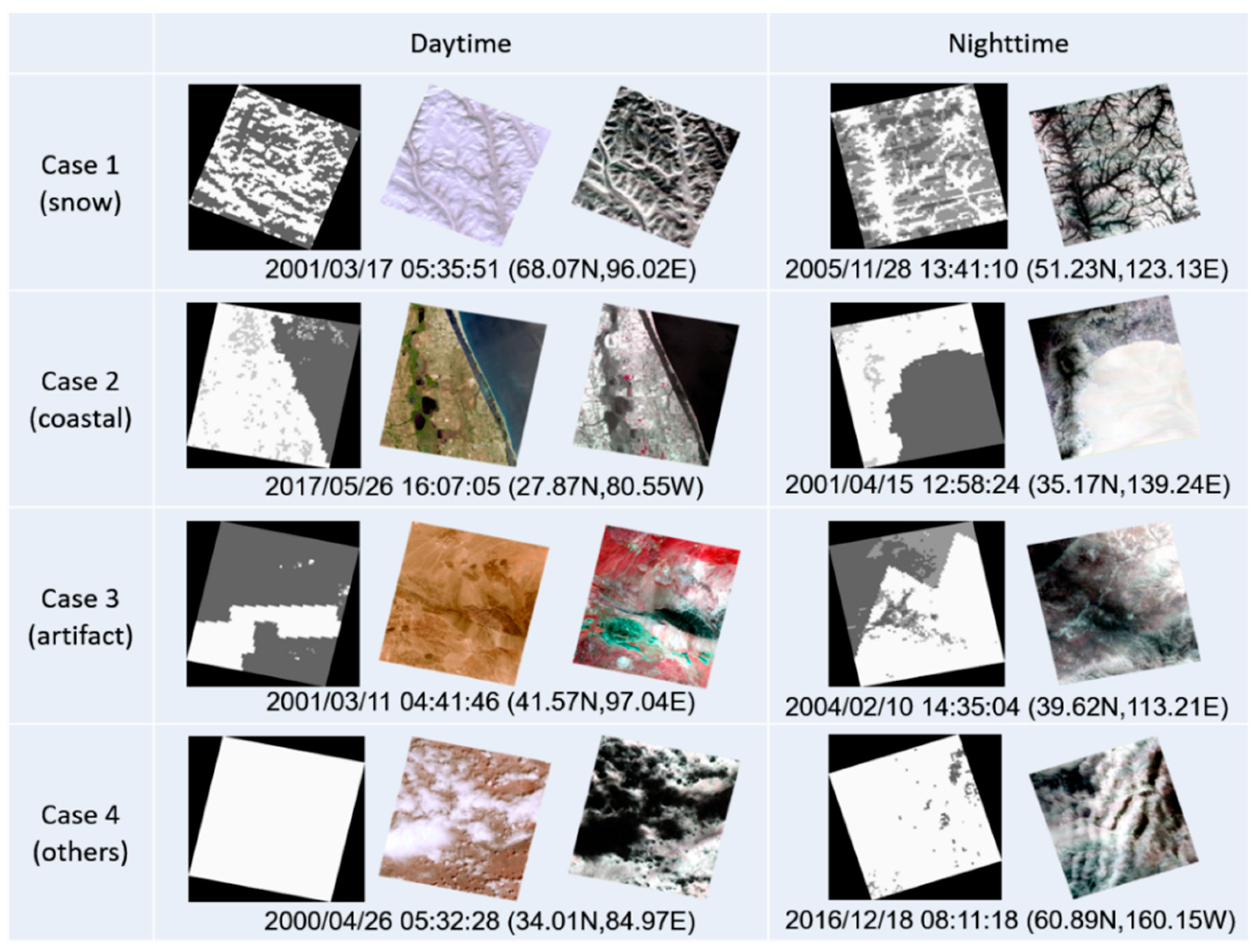
The visual evaluation of ASTER cloud mask images with browse images was performed for 24,706 daytime and 8006 nighttime scenes. As a result, 98.3% of daytime scenes (24,288) and 96.6% of nighttime scenes (7737) showed high consistency between cloud mask and browse images, leaving 1.7% of daytime and 3.4% of nighttime scenes with differences. As for 687 scenes with a problem, 31% of them were due to mislabeling in snow-covered areas (case 1), 19% of them were due to mislabeling of a water surface as a cloud in a coastal area (case 2), 15% of them were due to artifacts probably associated with ancillary data used in the MOD35 algorithm (case 3), and 35% of them were due to a large discrepancy in CC over surfaces such as ocean and desert (case 4). Figure 4 demonstrates examples of cases 1 to 4.
Thus, it should be noted that the above type of problems can be seen in a limited number of MOD35-based ASTER cloud masks, particularly in snow-covered or coastal areas.
3.2. ASTER Mission Operations Analysis Using MOD35-Based ASTER Cloud Masks
3.2.1. Validation of the Cloud Avoidance Function in the ASTER Observation Scheduler
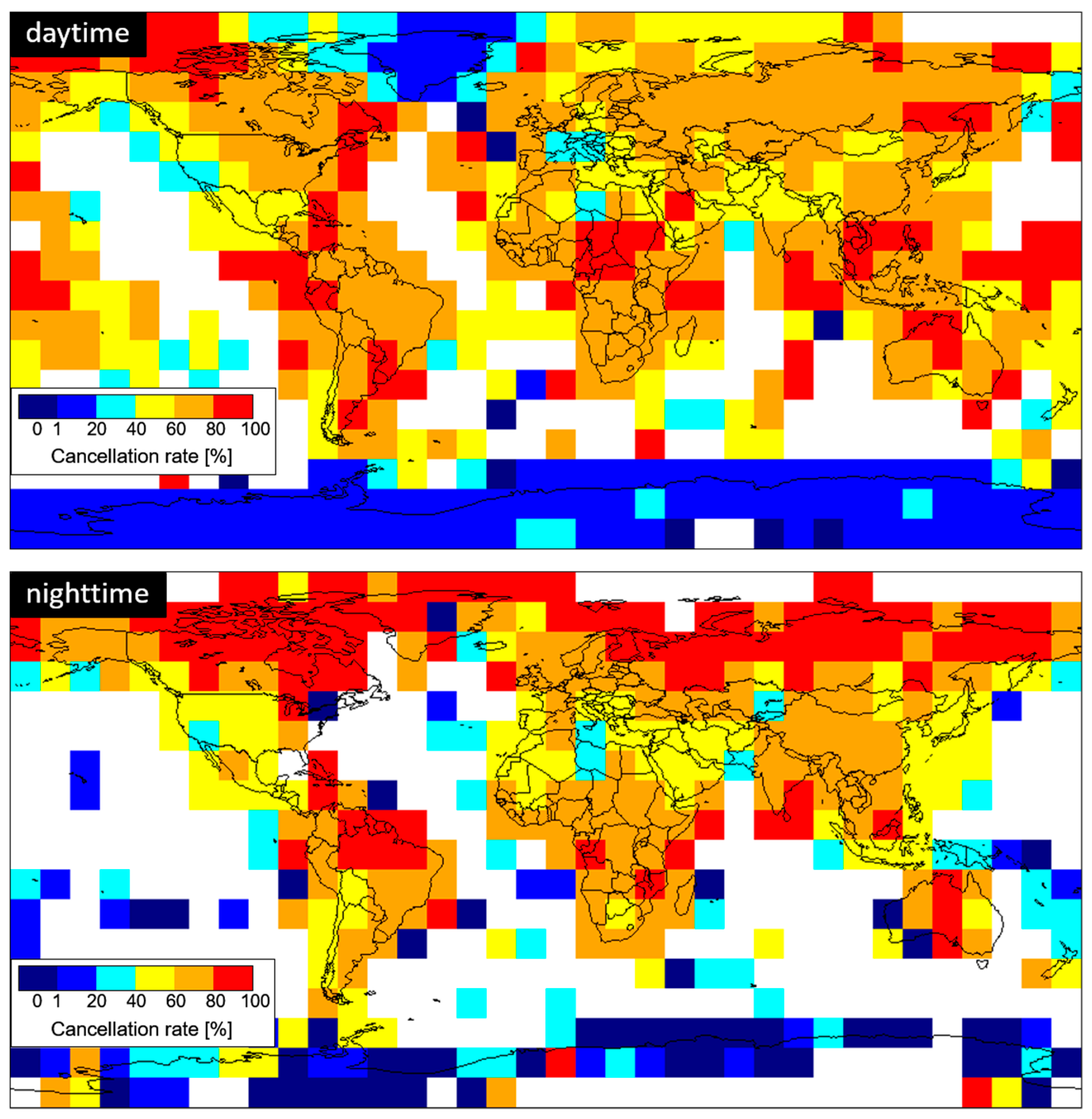
Figure 5 displays the cancellation rate of N-ODS for three years from 1 May 2016 to 30 April 2019 over 10 × 10 degree grids. As shown, observation cancels caused by the cloud avoidance function occur frequently in most of global land areas. In the west coast of USA, the cancellation rate is relatively low because this area is often observed by calibration-related requests without the cloud avoidance. As for Antarctica and Greenland, the cancellation rate in daytime is significantly low because these areas are frequently observed by requests without the cloud avoidance from the Global Land Ice Measurements from Space (GLIMS) Project [29].
Figure 6 gives the daily MCC values of “only N-ODS” and “only LC-ODS” as a function of date in daytime and nighttime. As shown, the TCC-based cloud avoidance function reduced the MCC significantly throughout the period, while it scatters more largely in nighttime. Table 3 gives the root mean square (RMS) differences of MCC and the clear-scene rate between N-ODS and LC-ODS for daytime and nighttime in the three years, where the clear-scene rate is defined as the rate of scenes with a CC of 20% or less. The table shows two cases that common scenes are included or not. Since the common scenes of N-ODS and LC-ODS account for about a half of the total scenes of LC-ODS in average as mentioned, the RMS differences with common scenes reduce by half, but the results show that the cloud avoidance function decreased MCC by 10% to 15% and increased the clear-scene rate by 10% to 15% even if common scenes are considered. The likely reason why the cloud avoidance function showed a better result in nighttime is probably because the subfunction f4 would affect ODS more strongly in nighttime due to fewer conflicts among fewer observation requests than in daytime.
Figure 7 displays the difference of MCC between “only LC-ODS” and “only N-ODS” over 10 × 10 degree grids for daytime and nighttime in the three years. If a grid cell has a negative difference, it means that LC-ODS has a smaller MCC than N-ODS, indicating the success of the cloud avoidance for that grid cell. As demonstrated by Figure 7, many grid cells are bluish, and reddish grid cells are limited in a small part of high latitude areas. This indicates that the cloud avoidance function performs well in most areas.
3.2.2. Time-Series Analysis of the Mean Cloud Coverage
Figure 8 shows the time-series satisfaction rate for global grid cells in daytime and nighttime, where the time-series satisfaction rate is defined as the rate of three-month terms including 10 scenes or more in a grid cell. The red grid cells are suitable for time-series analysis because they have been repeatedly observed in all seasons throughout 19 years, while the light purple or white grid cells are not suitable because observations are limited to a specific season or a part of the mission period. According to this result, we selected the following five grid cells, as shown in the figure: (A) USA, (B) Argentina, (C) Mozambique, (D) Indonesia, and (E) Japan.
Next, we performed seasonal decomposition with moving averages [26] for the MCC data at three-month intervals in the grid cells A to E, and divided the time-series data of each cell into the three components. As an example, Figure 9 displays the obtained time-series data at the grid cell E in daytime as follows: (a) the original MCC data, (b) the trend, (c) the seasonal change, and (d) the residual.
Figure 10 gives the trend plots of the three-monthly MCC values for the grid cells A to E in daytime and nighttime, also showing the trend plot of the monthly Niño 3.4 index. As shown, it appears that the fluctuations seen in the MCC trends can be partly explained by ENSO. For example, El Niño is often associated with warm and dry conditions around Indonesia [27]. The grid cell D, therefore, seems to have smaller MCC values in Niño events (positive in the monthly Niño 3.4 index), and larger MCC values in La Niña events (negative in the index).
Table 4 shows the means of the three-monthly MCC values for the five grid cells in daytime and nighttime over the period before the updating of κ (Period 1) and over the period after the updating (Period 2). The table also shows the difference between Periods 1 and 2 for each grid cell in daytime and nighttime. As demonstrated, the mean of the three-monthly MCC value in daytime is 0.5% to 7.9% smaller in Period 2 than in Period 1 for all grid cells in daytime and two grid cells (C and E) in nighttime, probably due to enhancement of the cloud avoidance function by updating of κ. The likely reason why the grid cells A, B, and D gave a positive difference in nighttime is due to weather fluctuations, although it is also noted that the high-uncertain rate is high around the grid cell D in nighttime (see Figure 3), and that the cancellation rate of N-ODS is low at the grid cell A (see Figure 5).
3.2.3. Mapping of the Number of Clear Scenes and the Success Rate
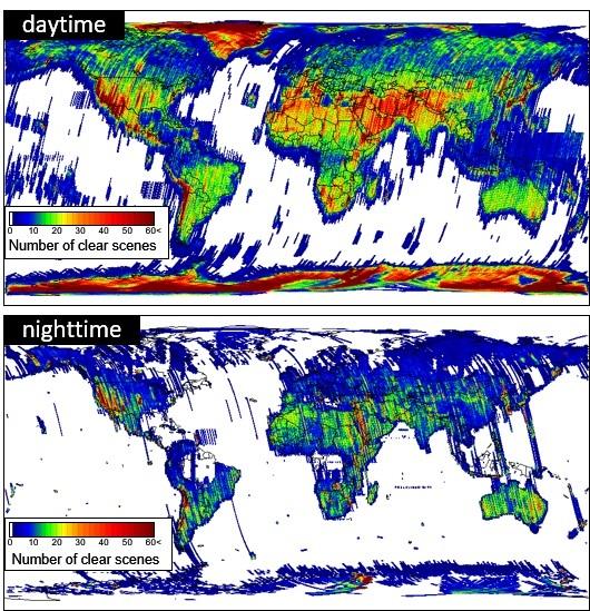
Figure 11 displays the daytime and the nighttime maps of the number of clear scenes over 10 × 10 degree grids in 19.5 years from March 2000 to August 2019, where a clear scene is defined as a scene with a CC of 20% or less. The overall mean values are 15.7 scenes in daytime, and 6.6 scenes in nighttime. In daytime, a large number of clear scenes can be seen in more frequently observed areas such as the west part of USA and Japan, in arid areas such as the Middle East, Sahara, the south of Africa, and the west coast of Central and South America, and in the polar areas with a narrower orbit spacing. Although the same tendency can be seen also in nighttime, the number of clear scenes is smaller in snow-covered or dense vegetated areas, because these areas have not been prioritized in nighttime scheduling.
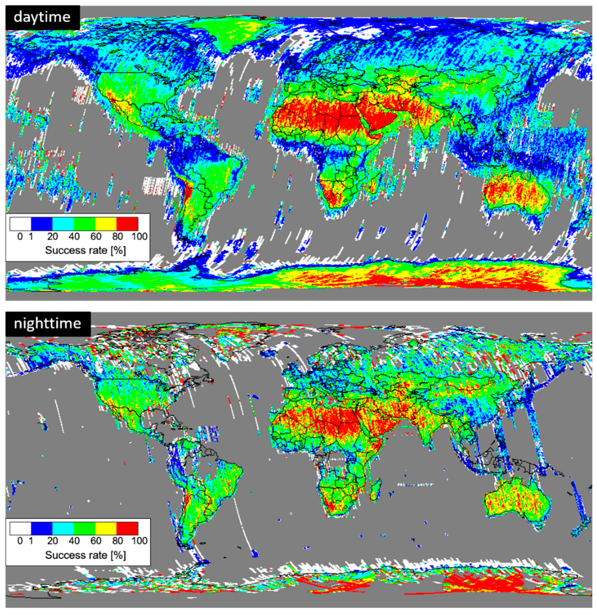
Figure 12 shows the daytime and the nighttime maps of the success rate over the same grids in the same period. The mean success rates in daytime and nighttime are 33.3% and 40.4%, respectively. The spatial distribution of the success rate is similar between daytime and nighttime, the rate is higher in arid areas, and lower in humid areas. The success rate in arid areas such as Sahara, Middle East, Australia, and Namibia is somewhat smaller in nighttime than in daytime, while that in high latitude areas is somewhat larger in nighttime.
4. Summary and Conclusions
Since the ASTER instrument cannot detect clouds accurately for snow-covered or nighttime images due to lack of spectral bands, the MOD35 product has been alternatively used in cloud assessment for all ASTER images. The most advantageous point of this approach is that the MODIS instrument onboard the same platform (Terra) always provides coincident and collocated observations using effective bands for cloud detection, although spatial resolution differences between ASTER and MODIS should be noted. In this study, we evaluated the reliability of MOD35-based ASTER cloud mask images, and then performed ASTER mission operations analysis using these cloud mask images.
For the evaluation of ASTER cloud mask images, we first compared them among different MOD35 versions. In updating from C5 to C6, the rates of ASTER scenes with the CC difference of 10% or greater (R10%) and with that of 50% or greater (R50%) were 18.5% and 6.5% in daytime, respectively, and 16.3% and 2.8% in nighttime, respectively. The likely cause of discrepancy between daytime and nighttime is a difference of observation areas. In updating from C6 to C6.1, R10% and R50% were about 2% and 0.4%, respectively, in both daytime and nighttime. Since C6 MOD35 products have been affected by an error on input L1B radiances, the ASTER Project has been generating cloud masks using C6.1 MOD35 products for all ASTER scenes.
Next, we analyzed the rate of uncertain pixels in each MOD35-based ASTER cloud mask image, because the uncertain flag in the MOD35 product can be used as a reliability index of cloud masks. The high-uncertain rate (the rate of scenes with the rate of uncertain pixels ≥30%) was 2.2% in daytime, and 12.0% in nighttime, indicating that the reliability of cloud masks is lower in nighttime. The results also indicate that the high-uncertain rate depends on location; daytime scenes have a large value in low-latitude areas, snow-covered areas, or some localized areas such as the north of Mozambique and the basin of Yellow River, and nighttime scenes have a large value in mountainous or glacier-lake areas. In addition, we evaluated MOD35-based ASTER cloud mask images visually using ASTER browse images for 24,706 daytime scenes and 8006 nighttime scenes. As a result, about 2% of the evaluated scenes showed some problems such as mislabeling in snow-covered or coastal areas, artifacts probably associated with ancillary data used in the MOD35 algorithm and mismatching in the cloud coverage.
With respect to ASTER mission operations analysis using MOD35-based ASTER cloud mask images, we first investigated the effectiveness of the TCC-based cloud avoidance function implemented in the ASTER observation scheduler. The analysis using N-ODS and LC-ODS data in the period from May 2016 to April 2019 showed that the cloud avoidance function canceled observations frequently in most of global land areas except for some areas frequently observed without the cloud avoidance function, such as the west area of North America, Antarctica and Greenland. Such canceled observation reduced MCC effectively in most areas, even if uncanceled scenes were considered, the cloud avoidance function decreased MCC by 10% to 15% and increased the rate of clear scenes by 10% to 15%. The time-series analysis of the three-monthly MCC values based on actual observations since the launch was also performed for the five grid cells (USA, Argentina, Mozambique, Indonesia, and Japan) in daytime and nighttime. Although the trend plots of MCC seem to have been partly affected by weather fluctuations, such as the ENSO, those plots showed a reduction of 0.5% to 7.9% in MCC between before and after April 2012 in which the coefficient κ in the cloud avoidance function was updated, except for three grid cells in nighttime. Finally, we generated the global maps of the number of clear scenes and the success rate using MOD35-based ASTER cloud mask images. The maps showed that the mean of the number of clear scenes was 15.7 scenes in daytime, and 6.6 scenes in nighttime, the mean success rate was 33.3% in daytime, and 40.4% in nighttime, and the success rate in arid areas was somewhat lower in nighttime than in daytime and that high-latitude areas had the opposite tendency.
Almost twenty years have passed since the ASTER instrument was launched in December 1999, and there are not many optical sensors with such a long-operation life. The results reported in this study are expected to contribute not only to the ASTER Project but also to other optical sensor projects.
Author Contributions
Conceptualization, H.T. and T.T.; methodology, H.T. and T.T.; software, H.T.; validation, H.T. and T.T.; formal analysis, H.T.; investigation, H.T. and T.T.; resources, H.T. and T.T.; data curation, H.T.; writing—original draft preparation, H.T.; writing—review and editing, H.T. and T.T.; visualization, H.T.; funding acquisition, T.T.
Funding
This research was funded by NASA Jet Propulsion Laboratory (USA).
Acknowledgments
The authors would like to thank the ASTER Science Team, particularly Michael Abrams (Jet Propulsion Laboratory, USA) and Yasushi Yamaguchi (Nagoya University, Japan) for giving comments on this study. Additional thanks to Yasushi Horiguchi and Akira Miura (Japan Space Systems) for providing useful information and data on the cloud avoidance function, and also to Yuki Koike, Mihiro Tsuda, Kazuki Ayuzawa, Yuki Kawamura, and Atsushi Tokida (Ibaraki University, Japan) for their supports with the visual evaluation of cloud mask images. The authors would also like to thank the editor and three anonymous reviewers for their comments and suggestions that greatly improved this manuscript.
Conflicts of Interest
The authors declare no conflict of interest.
References
- Yamaguchi, Y.; Kahle, A.B.; Tsu, H.; Kawakami, T.; Pniel, M. Overview of the advanced spaceborne thermal emission and reflectance radiometer (ASTER). IEEE Trans. Geosci. Remote Sens. 1998, 36, 1062–1071. [Google Scholar] [CrossRef]
- Yamaguchi, Y.; Abrams, M.J.; Kato, M.; Watanabe, H.; Tsu, H. ASTER science outcome and operation status. In Proceedings of the 2005 IEEE International Geoscience and Remote Sensing Symposium, Seoul, Korea, 29 July 2005; pp. 5578–5579. [Google Scholar] [CrossRef]
- Level 1 Data Working Group, ASTER Science Team. ASTER Algorithm Theoretical Basis Document for ASTER Level-1 Data Processing; Ver. 3.0; ERSDAC LEL/8-9; Earth Remote Sensing Data Analysis Center: Tokyo, Japan, 1996. Available online: http://eospso.gsfc.nasa.gov/sites/default/files/atbd/atbd-ast-01.pdf (accessed on 15 September 2019).
- Fujisada, H. ASTER level 1 data processing algorithm. IEEE Trans. Geosci. Remote Sens. 1998, 36, 1101–1112. [Google Scholar] [CrossRef]
- Irish, R. Landsat 7 automatic cloud cover assessment. In Algorithms for Multispectral, Hyperspectral, and Ultraspectral Imagery VI; International Society for Optics and Photonics: Bellingham, WA, USA, 2000; Volume 4049, pp. 348–355. [Google Scholar] [CrossRef]
- Tonooka, H.; Omagari, K.; Yamamoto, H.; Tachikawa, T.; Fujita, M.; Paitaer, Z. ASTER cloud coverage reassessment using MODIS cloud mask products. In Earth Observing Missions and Sensors: Development, Implementation, and Characterization; International Society for Optics and Photonics: Bellingham, WA, USA, 2010; Volume 7862. [Google Scholar] [CrossRef]
- Tonooka, H. ASTER nighttime cloud mask database using MODIS cloud mask (MOD35) products. In Remote Sensing of Clouds and the Atmosphere XIII; International Society for Optics and Photonics: Bellingham, WA, USA, 2008; Volume 7107. [Google Scholar] [CrossRef]
- Meyer, D.; Siemonsma, D.; Brooks, B.; Johnson, L. Advanced Spaceborne Thermal Emission and Reflection Radiometer Level 1 Precision Terrain Corrected Registered At-Sensor Radiance (AST_L1T) Product, Algorithm Theoretical Basis Document; Open-File Report 2015-1171; U.S. Geological Survey: Reston, VA, USA, 2015. [CrossRef]
- Hulley, G.C.; Hook, S.J. A new methodology for cloud detection and classification with ASTER data. Geophys. Res. Lett. 2008, 35, L16812. [Google Scholar] [CrossRef]
- Ackerman, S.A.; Strabala, K.I.; Menzel, W.P.; Frey, R.A.; Moeller, C.C.; Gumley, L.E. Discriminating clear sky from clouds with MODIS. J. Geophys. Res. 1998, 103, 32141–32157. [Google Scholar] [CrossRef]
- Ackerman, S.; Frey, R.; Strabala, K.; Liu, Y.; Gumley, L.; Baum, B.; Menzel, P. Discriminating Clear-Sky from Cloud with MODIS Algorithm Theoretical Basis Document (MOD35); Version 6.1; University of Wisconsin–Madison: Madison, WI, USA, 2010. Available online: https://modis-atmos.gsfc.nasa.gov/sites/default/files/ModAtmo/MOD35_ATBD_Collection6_0.pdf (accessed on 15 September 2019).
- LP DAAC. ASTER Cloud Cover Accuracy Improved. Available online: https://lpdaac.usgs.gov/news/aster-cloud-cover-accuracy-improved/ (accessed on 15 September 2019).
- Tonooka, H. ASTER Cloud Mask Database. Available online: http://tonolab.cis.ibaraki.ac.jp/ASTER/cloud/ (accessed on 15 September 2019).
- Ackerman, S.A.; Holz, R.E.; Frey, R.; Eloranta, E.W.; Maddux, B.C.; McGill, M. Cloud detection with MODIS. Part II: Validation. J. Atmos. Ocean. Technol. 2008, 25, 1073–1086. [Google Scholar] [CrossRef]
- Wilson, A.M.; Parmentier, B.; Jetz, W. Systematic land cover bias in Collection 5 MODIS cloud mask and derived products: A global overview. Remote Sens. Environ. 2014, 141, 149–154. [Google Scholar] [CrossRef]
- Wang, T.; Fetzer, E.J.; Wong, S.; Kahn, B.H.; Yue, Q. Validation of MODIS cloud mask and multilayer flag using CloudSat-CALIPSO cloud profiles and a cross-reference of their cloud classifications. J. Geophys. Res. Atmos. 2016, 121, 11620–11635. [Google Scholar] [CrossRef]
- Moeller, C.; Frey, R. Terra MODIS Collection 6.1 Calibration and Cloud Product Changes, Version 1.0 (27 June 2017). Available online: https://modis-atmos.gsfc.nasa.gov/sites/default/files/ModAtmo/C6.1_Calibration_and_Cloud_Product_Changes_UW_frey_CCM_1.pdf (accessed on 15 September 2019).
- Muraoka, H.; Cohen, R.H.; Ohno, T.; Doi, N. ASTER observation scheduling algorithm. In Proceedings of the International Symposium Space Mission Operations and Ground Data Systems, Tokyo, Japan, 1–5 June 1998. [Google Scholar]
- King, M.D.; Platnick, S.; Menzel, W.P.; Ackerman, S.A.; Hubanks, P.A. Spatial and temporal distribution of clouds observed by MODIS onboard the Terra and Aqua satellites. IEEE Trans. Geosci. Remote Sens. 2013, 51, 3826–3852. [Google Scholar] [CrossRef]
- Frey, R.A.; Acherman, S.A.; Liu, Y.; Strabala, K.I.; Zhang, H.; Key, J.R.; Wang, X. Cloud detection with MODIS. Part I: Improvements in the MODIS cloud mask for Collection 5. J. Atmos. Ocean. Technol. 2008, 25, 1057–1072. [Google Scholar] [CrossRef]
- Frey, R. Collection 6 Updates to the MODIS Cloud Mask (MOD35). 2010. Available online: https://modis.gsfc.nasa.gov/sci_team/meetings/201001/presentations/atmos/frey.pdf (accessed on 15 September 2019).
- Wilson, T.; Wu, A.; Shrestha, A.; Geng, X.; Wang, Z.; Moeller, C.; Frey, R.; Xiong, X. Development and implementation of an electronic crosstalk correction for bands 27–30 in Terra MODIS collection 6. Remote Sens. 2017, 9, 569. [Google Scholar] [CrossRef]
- Level-1B (L1B) Calibration, Collection 6.0 and Collection 6.1 Changes, Terra and Aqua MODIS. Available online: https://atmosphere-imager.gsfc.nasa.gov/sites/default/files/ModAtmo/C061_L1B_Combined_v10.pdf (accessed on 15 September 2019).
- MODIS/Terra Data Outages. Available online: https://modaps.modaps.eosdis.nasa.gov/services/production/outages_terra.html (accessed on 15 September 2019).
- NOAA/National Weather Service, National Centers for Environmental Prediction, Environmental Modeling Center. Global Forecast System (GFS). Available online: https://www.emc.ncep.noaa.gov/GFS/ (accessed on 15 September 2019).
- Seabold, S.; Perktold, J. Statsmodels: Econometric and statistical modeling with python. In Proceedings of the 9th Python in Science Conference (SciPy 2010), Austin, TX, USA, 28–30 June 2010. [Google Scholar]
- World Meteorological Organization. El Niño/Southern Oscillation. WMO-No.1145. 2014. Available online: http://www.wmo.int/pages/prog/wcp/wcasp/documents/JN142122_WMO1145_EN_web.pdf (accessed on 15 September 2019).
- NOAA/National Weather Service, Climate Prediction Center. Historical El Nino/La Nina episodes (1950–present). Available online: https://origin.cpc.ncep.noaa.gov/products/analysis_monitoring/ensostuff/ONI_v5.php (accessed on 15 September 2019).
- Raup, B.H.; Racoviteanu, A.; Khalsa, S.J.S.; Helm, C.; Armstrong, R.; Arnaud, Y. The GLIMS geospatial glacier database: A new tool for studying glacier change. Glob. Planet. Chang. 2007, 56, 101–110. [Google Scholar] [CrossRef]
Figure 1.
Scheduled areas included in only normal one-day schedule “(N-ODS)”, only late change one-day schedule “(LC-ODS)”, and both N-ODS and LC-ODS (“common”) on 7 April 2018. The background is the daily cloud fraction image from the MODIS MOD08 product on the same day (blue, cloud and white, clear).

Figure 2.
Difference of ASTER CC between different MOD35 versions as a function of latitude. (a) C6 minus C5 in daytime, (b) C6 minus C5 in nighttime, (c) C6.1 minus C6 in daytime, and (d) C6.1 minus C6 in nighttime. A total of 17,845 daytime scenes and 8521 nighttime scenes observed in 2016 were used.

Figure 3.
C6.1-based high-uncertain rate maps over 0.1 × 0.1 degree grids for daytime and nighttime using all ASTER archives as of 10 August 2019.
Figure 3.
C6.1-based high-uncertain rate maps over 0.1 × 0.1 degree grids for daytime and nighttime using all ASTER archives as of 10 August 2019.

Figure 4.
Examples of ASTER cloud mask images with a problem in visual evaluation for daytime and nighttime for case 1 (snow/ice area), case 2 (coastal waters), case 3 (artifact), and case 4 (others including ocean and desert). Images in each cell are the cloud mask image (left), the visible and near-infrared (VNIR) browse image (middle, only daytime; BGR = bands 1, 2, and 3N), and the thermal infrared (TIR) browse image (right; BGR = bands 10, 12, and 14). White, dark gray, and black on each cloud mask image indicate clear, cloud, and background, respectively.

Figure 5.
Cancellation rate of N-ODS for three years from 1 May 2016 to 30 April 2019 over 10 × 10 degree grids for each of daytime and nighttime.
Figure 5.
Cancellation rate of N-ODS for three years from 1 May 2016 to 30 April 2019 over 10 × 10 degree grids for each of daytime and nighttime.

Figure 6.
Daily mean cloud coverage (MCC) values of “only N-ODS” and “only LC-ODS” as a function of date in the three years from 1 May 2016 to 30 April 2019.
Figure 6.
Daily mean cloud coverage (MCC) values of “only N-ODS” and “only LC-ODS” as a function of date in the three years from 1 May 2016 to 30 April 2019.

Figure 7.
Difference of MCC between “only LC-ODS” and “only N-ODS” over 10 × 10 degree grids for daytime and nighttime in the three years from 1 May 2016 to 30 April 2019. In bluish cells, “only LC-ODS” has a smaller MCC than “only N-ODS”, indicating the success of the cloud avoidance function.
Figure 7.
Difference of MCC between “only LC-ODS” and “only N-ODS” over 10 × 10 degree grids for daytime and nighttime in the three years from 1 May 2016 to 30 April 2019. In bluish cells, “only LC-ODS” has a smaller MCC than “only N-ODS”, indicating the success of the cloud avoidance function.

Figure 8.
Time-series satisfaction rate for global grid cells in daytime and nighttime. The five grid cells used for the time-series analysis are also shown.
Figure 8.
Time-series satisfaction rate for global grid cells in daytime and nighttime. The five grid cells used for the time-series analysis are also shown.

Figure 9.
Time-series data at the grid cell E in daytime as an example: (a) the original MCC data, (b) the trend, (c) the seasonal change, and (d) the residual.
Figure 9.
Time-series data at the grid cell E in daytime as an example: (a) the original MCC data, (b) the trend, (c) the seasonal change, and (d) the residual.

Figure 10.
Trend plots of the three-monthly MCC values for the grid cells A to E in daytime and nighttime, also showing the trend plot of the monthly Niño 3.4 index.
Figure 10.
Trend plots of the three-monthly MCC values for the grid cells A to E in daytime and nighttime, also showing the trend plot of the monthly Niño 3.4 index.

Figure 11.
Daytime and nighttime maps of the number of clear scenes with a CC of 20% or less over 10 × 10 degree grids in 19.5 years from March 2000 to August 2019.
Figure 11.
Daytime and nighttime maps of the number of clear scenes with a CC of 20% or less over 10 × 10 degree grids in 19.5 years from March 2000 to August 2019.

Figure 12.
Daytime and nighttime maps of the success rate over 10 × 10 degree grids in 19.5 years from March 2000 to August 2019.
Figure 12.
Daytime and nighttime maps of the success rate over 10 × 10 degree grids in 19.5 years from March 2000 to August 2019.


Table 1.
Spectral range and ground resolution of each Advanced Spaceborne Thermal Emission and Reflection Radiometer (ASTER) spectral band [1].
Table 1.
Spectral range and ground resolution of each Advanced Spaceborne Thermal Emission and Reflection Radiometer (ASTER) spectral band [1].
| Subsystem | Spectral Range [μm] | Ground Resolution |
|---|---|---|
| VNIR | Band 1: 0.52−0.60 Band 2: 0.63−0.69 Band 3N, 3B: 0.78−0.86 | 15 m |
| SWIR | Band 4: 1.600−1.700 Band 5: 2.145−2.185 Band 6: 2.185−2.225 Band 7: 2.235−2.285 Band 8: 2.295−2.365 Band 9: 2.360−2.430 | 30 m |
| TIR | Band 10: 8.125−8.475 Band 11: 8.475−8.825 Band 12: 8.925−9.275 Band 13: 10.25−10.95 Band 14: 10.95−11.65 | 90 m |
Table 2.
Mean of the CC difference (bias), R10%, and R50% in daytime and nighttime for C6 minus C5 and C6.1 minus C6.
Table 2.
Mean of the CC difference (bias), R10%, and R50% in daytime and nighttime for C6 minus C5 and C6.1 minus C6.
| Parameter | C6 Minus C5 | C6.1 Minus C6 | ||
|---|---|---|---|---|
| Daytime | Nighttime | Daytime | Nighttime | |
| bias | −5.7% | −1.4% | −0.6% | −0.6% |
| R10% | 18.5% | 16.3% | 1.9% | 2.1% |
| R50% | 6.5% | 2.8% | 0.4% | 0.3% |
Table 3.
RMS differences of MCC and the clear-scene rate between N-ODS and LC-ODS for daytime and nighttime in the three years. Two cases that common scenes are included or not are shown.
Table 3.
RMS differences of MCC and the clear-scene rate between N-ODS and LC-ODS for daytime and nighttime in the three years. Two cases that common scenes are included or not are shown.
| Day/Night | RMS Difference of MCC | RMS Difference of Clear-scene Rate | ||
|---|---|---|---|---|
| no Common | with Common | no Common | with Common | |
| daytime | 20.1% | 11.4% | 21.5% | 12.3% |
| nighttime | 25.3% | 15.4% | 25.8% | 15.8% |
Table 4.
The means of the three-monthly MCC values for the grid cells A to E in daytime and nighttime over the period before the updating of κ in Equation (1) (Period 1) and over the period after the updating (Period 2). The difference between Periods 1 and 2 in each case is also shown.
Table 4.
The means of the three-monthly MCC values for the grid cells A to E in daytime and nighttime over the period before the updating of κ in Equation (1) (Period 1) and over the period after the updating (Period 2). The difference between Periods 1 and 2 in each case is also shown.
| Grid Cell | Daytime | Nighttime | ||||
|---|---|---|---|---|---|---|
| Period 1 | Period 2 | diff. | Period 1 | Period 2 | diff. | |
| (A) USA | 29.1 | 23.3 | −5.8 | 24.2 | 26.0 | 1.8 |
| (B) Argentina | 24.0 | 18.3 | −5.7 | 25.6 | 26.3 | 0.7 |
| (C) Mozambique | 39.0 | 31.2 | −7.9 | 33.7 | 27.4 | −6.3 |
| (D) Indonesia | 60.7 | 60.3 | −0.5 | 64.0 | 67.8 | 3.8 |
| (E) Japan | 64.9 | 59.4 | −5.4 | 66.7 | 62.8 | −3.9 |
© 2019 by the authors. Licensee MDPI, Basel, Switzerland. This article is an open access article distributed under the terms and conditions of the Creative Commons Attribution (CC BY) license (http://creativecommons.org/licenses/by/4.0/).
Share and Cite
MDPI and ACS Style
Tonooka, H.; Tachikawa, T. ASTER Cloud Coverage Assessment and Mission Operations Analysis Using Terra/MODIS Cloud Mask Products. Remote Sens. 2019, 11, 2798. https://doi.org/10.3390/rs11232798
AMA Style
Tonooka H, Tachikawa T. ASTER Cloud Coverage Assessment and Mission Operations Analysis Using Terra/MODIS Cloud Mask Products. Remote Sensing. 2019; 11(23):2798. https://doi.org/10.3390/rs11232798
Chicago/Turabian StyleTonooka, Hideyuki, and Tetsushi Tachikawa. 2019. "ASTER Cloud Coverage Assessment and Mission Operations Analysis Using Terra/MODIS Cloud Mask Products" Remote Sensing 11, no. 23: 2798. https://doi.org/10.3390/rs11232798
Note that from the first issue of 2016, this journal uses article numbers instead of page numbers. See further details here.