Modelling Three-Dimensional Spatiotemporal Distributions of Forest Photosynthetically Active Radiation Using UAV-Based Lidar Data


1
International Institute for Earth System Science, Nanjing University, Nanjing 210023, China
2
Jiangsu Provincial Key Laboratory of Geographic Information Science and Technology, Nanjing 210023, China
3
Institute of Forest Resource Information Techniques, Chinese Academy of Forestry, No.2 Dongxiaofu, Haidian District, Beijing 100091, China
*
Author to whom correspondence should be addressed.
Remote Sens. 2019, 11(23), 2806; https://doi.org/10.3390/rs11232806
Submission received: 20 September 2019
/
Revised: 25 November 2019
/
Accepted: 26 November 2019
/
Published: 27 November 2019
(This article belongs to the Special Issue Lidar Remote Sensing of Forest Structure, Biomass and Dynamics)
Abstract
:The three dimensional (3-D) spatiotemporal variations of forest photosynthetically active radiation (PAR) dictate the exchange rates of matter and energy in the carbon and water cycle processes between the plant-soil system and the atmosphere. It is still challenging to explicitly simulate spatial PAR values at any specific position within or under a discontinuous forest canopy. In this study, we propose a novel lidar-based approach to estimate both direct and diffuse forest PAR components from a 3-D perspective. An improved path length-based direct PAR estimation method was developed by incorporating the point density along a light transmission path, and we also obtained the diffuse PAR components using a point-based sky view analysis by assuming the anisotropic sky diffuse distribution. We compared the total PAR modelled using three light path length-based parameters with reference data measured by radiometers on a five-minute time scale during a daily solar course. Our results show that, in a discontinuous forest canopy, the effective path length is a feasible and powerful (R2 = 0.92, p < 0.01) parameter to capture the spatiotemporal variations of total PAR along a light transmission path with a mean bias of −53.04 μmol·m−2·s−1(−6.8%). Furthermore, incorporating point density and spatial distribution factors will further improve the final estimation accuracy (R2 = 0.97, p < 0.01). In the meantime, diffuse PAR tends to be overestimated by 17% at noon and underestimated by about 10% at sunrise and sunset periods by assuming the isotropic sky diffuse distribution. The proposed lidar-based 3-D PAR model will provide a solid foundation to various process-based eco-hydrological models for simulating plant physiological processes such as photosynthesis and evapotranspiration, intra-species competition and succession, and snowmelt dynamics purposes.
1. Introduction
The forest radiation regime is the basic driving factor for most physiological processes such as photosynthesis and respiration [1,2]. The spatiotemporal distributions of forest photosynthetically active radiation (PAR, 400~700 nm) in the three dimensional (3-D) space has great effects on sub-canopy snowmelt dynamics [3,4], understory evapotranspiration [5,6], and the growth and succession of tree seedlings [7,8]. It is determined by absorbing, scattering, and transmitting processes between solar PAR and foliage elements as it penetrates through a forest canopy [9,10]. These processes are dominated by factors including leaf orientation and morphology, the distribution pattern of foliage elements, solar position, and topographic conditions [11,12]. Extremely high heterogeneity could usually be observed for spatiotemporal distributions of forest PAR in both horizontal and vertical dimensions, especially at a sub-daily scale [13,14].
The spatiotemporal variations of PAR could be conventionally and directly measured by pyranometers [15,16] and indirectly observed by digital hemispherical photography (DHP) [17,18,19] at different locations within a forest plot. However, it is difficult to set up a pyranometer observation network or to obtain DHPs in large or inaccessible forested areas, and the high spatial heterogeneity of PAR in complex forest areas cannot be effectively represented by data at specific sampling points. Therefore, their applications can’t be extended to larger spatial scales. To solve this issue, canopy light models became a powerful tool to investigate the 3-D spatiotemporal distributions of forest PAR [20]. The spatially explicit 3-D radiative transfer models have been developed in the past decades for non-randomly distributed heterogeneous forest canopies. They included the Beer law-based radiative transfer model [21,22,23], and the ray tracing model using Monte-Carlo simulation [24,25,26]. The Beer-Lambert law describes the exponential attenuation of solar radiation, and it is only applicable to situations where randomly distributed foliage elements can be assumed [27]. The detailed 3-D structure information of forest canopies is a prerequisite input for these computer-based models. For example, some models represented the tree crowns using different geometric objects such as a cone or cylinder, and the direct light could be traced during the daily solar course [28,29,30]. However, it is usually extremely time-consuming and labor-intensive to obtain forest canopy structural parameters such as tree height, diameter at breast height (DBH), crown size, and crown base height [14]. Moreover, compared with the real 3-D forest scene, the artificially reconstructed forest scene usually fails to capture the real gap distribution patterns, which makes the modelled radiation at the specific location deviate from the actual PAR values [31,32]. In addition, previous studies have shown that the estimation accuracy of aerial laser scanning (ALS)-derived forest canopy structural parameters will decrease slightly as data point density decreases [33,34]. However, how the point cloud density affects the accuracy of ALS-based 3-D canopy light models remains unclear.
An accurate description of the tree structure is the key step to simulating the radiation regime of a forest canopy. With the development of light detection and ranging (lidar) technology, a detailed 3-D structure represented by lidar-based high-density point cloud data can be acquired efficiently. ALS has shown great potential for forest ecological applications at the landscape level [35,36]. To investigate the radiation regime of forest canopies, several ALS-based 3-D canopy light models have been successfully developed over the past decades [32,37,38]. Most of these models characterize the probability of direct or diffuse solar radiation penetrating through forest canopies based on various lidar-derived metrics such as the laser penetration index [39], leaf area density [40], point projection area on the ground surface [41], number of points around a solar ray [42], and synthetic hemispherical images derived from projected point cloud data [43,44]. More detailed 3-D canopy light models have been developed based on terrestrial laser scanning (TLS) to simulate radiation transmittance by voxel-based canopy reconstruction [45,46]. As a bridge linking ALS and TLS, unmanned aerial vehicle (UAV)-based lidar systems provide great flexibility in selecting data point density, as well as better delineation to the upper part of a canopy with top-down scanning [47,48]. However, a 3-D forest canopy radiation model driven by high-density UAV-based lidar data remains a necessary development.
The PAR arriving at one point in the forest canopy mainly consists of direct components originating from the transmission and attenuation of beams and diffuse components derived from single and multiple scattering. Naturally, most canopy light models simulate them separately [12,39]. In terms of direct solar radiation, the length of the transmission path, defined as the distance between the first contacted point and the target point [13,30], is a widely used parameter to determine the extent of its potential attenuation [14,29]. It was found that a path-length based radiation simulation model is more flexible in terms of reproducing sub-daily and seasonal PAR variations [49]. Moreover, existing research found that a spatially explicit 3-D ray trace model incorporating path length could simulate the spatiotemporal distribution patterns of light intensity in the forest floor and along the vertical gradient [14]. However, it is usually not good enough to only consider the total path length to accurately characterize the light attenuation effect along its transmission path due to the non-random distribution of foliage elements within a forest canopy [50]. The gaps between clumped foliage elements along a light transmission path will alter their attenuation ability for direct solar radiation. In addition, the point density and distribution pattern along a light transmission path will also affect the ability of a direct beam penetrating through a forest canopy [33,51]. However, few studies have incorporated the gap size information into the path length-based method to characterize the light attenuation, and it is still unclear whether it is possible to improve the simulation accuracy of the light attenuation effect by incorporating the point density and distribution information. In terms of diffuse components, most research treats the diffuse light above the hemispherical sky as an isotropic distribution. The diffuse solar radiation reaching a specific location in a forest canopy is usually estimated based on the sky view factor or canopy closure [15,19,49]. To assume the isotropic diffuse solar radiation will affect the estimated radiation regime in 3-D space [52,53], while the difference remains unexplored.
Therefore, in this study, we aimed to develop a spatially explicit forest canopy radiation model to investigate the spatiotemporal variations of forest PAR within and under a forest canopy. The specific objectives of this study are to:
- Develop and validate a spatially explicit lidar-based 3-D forest canopy PAR simulation model treating direct and diffuse solar radiation separately;
- Characterize the attenuation effects of direct solar PAR along its transmission path penetrating through a forest canopy, and
- Explore the spatiotemporal variations of forest PAR in 3-D space and the effects of point density on the estimation accuracy of forest PAR simulation.
2. Materials and Methods
2.1. Study Sites
Our study area is located in the Baima (BM) experimental forest site in the city of Nanjing (119°11′8″E, 31°36′51″N), China (Figure 1). The site is a planted forest site with a relatively flat area and different tree species, densities, and ages. We set up a medium density (0.15 trees / m2) deciduous broadleaf circular forest plot with a radius of 15 m. The average tree height and crown size of this forest plot are 7 m and about 2~3 m, respectively. The effective leaf area index (LAIe) is about 1.5. The tree species of this forest plot is wheel wingnut (Cyclocarya paliurus) with an average spacing of 2 m between tree stems.
2.2. Data Collection
2.2.1. UAV Lidar Data
We acquired the UAV-based lidar data in the BM site on July 26, 2017 on a clear day with the DJI M600 pro (DJI Technology Co. Ltd, Shenzhen, China) drone mounted with a Velodyne VLP-16 (Velodyne LiDAR Inc. San Jose, USA) lidar sensor coupled with a high precision inertial measurement unit (IMU). The scanning field of view (FOV) was set as ±15° with the laser wavelength of 903 nm and beam divergence of 0.18° (3.0 mrad) during the flight. The maximum scan rate of the lidar sensor was 300,000 points/s. Two cross flight paths (i.e., East-West and North-South) were designed to acquire relatively comprehensive forest point cloud data, which resulted in high-density (about 500 points/sqm) 3-D forest point cloud data (Figure 1b).
2.2.2. TLS Data
In the meantime, we also collected terrestrial lidar data using the Leica Scan Station 2 (Leica Geosystem AG, St. Gallen, Switzerland) at five different scanning locations with one center position and four corner positions, respectively. At each station, we scanned the plot using hemispherical mode (i.e., horizontal: 0~360°; vertical: −45~90°) by setting sampling spacing as 1 cm @ 10 m (1 cm at 10 m away from TLS station) with the laser wavelength of 532 nm. All TLS data from five different stations were registered into a comprehensive forest plot TLS point cloud.
2.2.3. Lidar Data Pre-Processing
In this study, we filtered ground points for both UAV and TLS lidar data using the tool ‘CSF’ in the ‘CloudCompare’ software package (version 2.6.2) (GPL software and available from http://cloudcompare.org). Then, the digital elevation model (DEM) and canopy height model (CHM) with the spatial resolution of 0.1 m were interpolated in ArcGIS software using ground points from UAV lidar data. In addition, after removing the noise points of TLS data, we removed all points lower than each PAR observation location to estimate the sky view factor for diffuse solar radiation calculation purposes. Accurately locating the observation points in 3-D both UAV- and TLS-based lidar data is a key step to assure the effectiveness of comparison between the lidar- and field-based PAR values. All nine observation locations were precisely captured by TLS data. By visually selecting two control points in both UAV- and TLS- lidar data space, we first calculated distances from each observation location to these two control points. Then, by using the distance intersection method we successfully located nine observation locations in the UAV-lidar data space (Table 1).
2.2.4. Field-Based PAR Measurements
Nine different light quantum sensors recorded photosynthetic photon flux density (PPFD) (μmol·m−2·s−1) with the average logging time interval of 5 minutes and heights of 1~2 m above the ground at different locations at the BM site from July 27 to July 28, 2017. In the meantime, we also measured the total () and diffuse PAR () above forest canopy using the BF-5 sunshine sensor (Delta-T Devices Ltd., Cambridge, UK) placed on a roof 20 meters above the ground. By doing so, we obtained the direct PAR () by subtracting from .
2.2.5. PAR Measurements Normalization
To compare the PAR measurements from nine different light sensors, we conducted the data calibration process using a standard reference light quantum sensor (LI-190R, LI-COR, Inc., Lincoln, Nebraska) under the same light condition and indoor environment. By sampling the PAR readings from the to-be-calibrated sensor with the reference one at a step of 50 μmol·m−2·s−1 within the range from 0 to 2500 μmol·m−2·s−1, we calculated the difference between two readings. The quadratic polynomial statistical model best explains the variations of reference PAR measurements with the to-be-calibrated measurements with significant correlations (R2 = 0.99 and P < 0.01) and is expressed as:
where is the difference of PPFD between the i-th pyranometer and LI-190R, is the corresponding PPFD of LI-190R, and , and are calibration coefficients for the i-th pyranometer as shown in Table 1.
2.3. Model Development
We developed a lidar-based radiation model based on the following assumptions: (1) The total solar radiation () reaching a specific location within or under a forest canopy in 3-D space consists of both the direct PAR () and diffuse PAR () components. (2) The solar radiation reaching a specific location is mainly determined by the non-random distributions of foliage elements within the 3-D space of a forest canopy which is represented by UAV-lidar data in this study. The solar radiation absorbed by leaves was ignored in this study. We calculated the direct PAR (), diffuse PAR () and scattering PAR () components separately.
2.3.1. Direct PAR Estimation Model
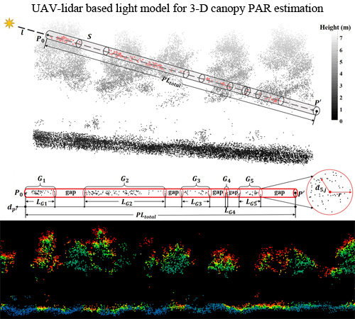
In the current study, we developed a lidar-based approach to characterize the attenuation of direct solar radiation along their transmission path as penetrating through a forest canopy. As shown in the Figure 2, for a given direct light beam l with the zenith (Z) and azimuthal (A) angles reaching a given target point , we could build a 3-D cylindrical buffer (S) region around the light beam l with the radius of r as it penetrates through a forest canopy. The radius r was determined by the sensitivity analysis in Section 2.4. The 3-D cylindrical buffer could be either occupied by points (i.e., “vegetation cluster”) or empty (i.e., “gaps”) resulting from non-random distribution of foliage elements. We projected each point within the buffer S onto the light beam l and computed their one-dimensional distances between each projected point and point along l (). The point with the longest was considered as the first contact point between light beams and forest canopy (). We then applied the K-Means++ algorithm [54] to group the vegetation points and identify the gaps between foliage elements within the buffer S. The initial number of clusters (k) was set as half of the total number of points (N) within S, and the buffer was considered as an empty one if N was less than 2. Two clusters would be merged if the distance between their boundaries was less than 0.5 m determined by measuring the mean gap size manually. By iteratively clustering all points within the buffer S, we obtained five “vegetation clusters” (~) and five “gaps” with varied sizes in the buffer S, respectively.
The direct PAR values at the point could be obtained if the attenuation effects of direct light beams could be characterized as they penetrate through a forest canopy. By removing the gaps from the buffer S whose total path length is , we computed the effective total path length () as:
where is the length for the i-th vegetation cluster cylinder; is the total path length of direct light beam starting from the first contacted point within forest canopy () to the target point . As for the value of , it could be computed as:
where is the distance of each point within the i-th vegetation cluster between its projected point and the target point along l, and and are the maximum and minimum distances, respectively. To better characterize the non-distribution pattern of foliage elements along the light transmission path, besides the path length, we also proposed another parameter named the point density-based length () to characterize the light attenuation effect by incorporating the point density and spatial distribution pattern within vegetation clusters. The relative volume point density () of the i-th separated vegetation cluster is computed as:
where is the average point density of tree crowns in the study area with the unit of points/m3, is the total number of points contained in , r is the radius of the cross-sectional circle of the cylindrical buffer S, and is the length of the vegetation cluster . We determined the value of by averaging the point volume density of 50 randomly selected spheres with a radius of 0.5 m within tree crowns. For the vegetation clusters with extremely high or low densities along all possible direct beams reaching the target point , we plotted the histogram of all values during a daily solar course and replaced abnormal (i.e., extremely large or small) values using the ones at the point of 95% confidence interval.
In addition, the 3-D spatial distribution patterns of all points within each also affect the attenuation effects of direct solar beams. By assuming that the ability to intercept direct solar radiation was inversely related with the distances of each point to the axis of 3-D cylindrical buffer S, we proposed a parameter named “relative point distribution factor ()” to characterize the spatial distribution pattern of points within vegetation clusters. In each vegetation cluster , the value of was computed as:
where is the distance of the j-th point within the i-th vegetation cluster to the axis of cylindrical buffer S and is the total number of points within . We obtained the average value based on all possible values of for all direct beams reaching nine observation points during a daily solar course.
and are the absolute volume point density and the absolute point distribution factor for the i-th vegetation cluster, respectively. Statistically, they approximately show a normal distribution with or as the mean value, so the values of and exhibit a positively skewed distribution with the mode of 1. When both and are equal to 1, we call it the standard case. A value greater than 1 indicates that more foliage elements exist in the cluster , enhancing its attenuation effects compared to the standard case. Meanwhile, a value greater than 1 indicates that more foliage elements are located closer to the light path in the cluster and has the same effects as . Finally, we computed the value of point density-based path length () weighted by the point volume density and point spatial distribution pattern as:
In terms of the direct PAR reaching the target point , we applied an exponent-based direct light attenuation model as:
where , , and are unknown coefficients for the exponent statistical model and is one of the three light path length-based parameters (, , ). To determine the unknown parameters, we conducted the non-linear regression analysis based on the No. 5 and No. 6 pyranometer measurements in the field to fit the exponential model between and direct light transmittance (). We obtained the observed by subtracting the and from the pyranometer readings during a daily solar course.
2.3.2. Diffuse PAR Estimation Model
The sky diffuse distributes ununiformly in the upper hemisphere under a clear sky condition and it was controlled by the solar position. In this study, we incorporated our diffuse sky model with an anisotropic sky diffuse distribution model [52]. The model describes the variation of relative contributions of sky diffuse irradiance in each zenith-angle zone to horizontal irradiance with the various solar positions under clear sky conditions. We divided the upper hemisphere into nine zenith-angle zones with a 10° zenith angle interval, and their relative contributions varying with the solar zenith angle are shown in Figure 3.
The angular gap fraction is defined as the proportion of partial or whole hemispherical sky not obscured by foliage elements of a forest canopy when viewed upwards from a specific location [55]. To calculate , the gap fraction of each annulus zone needs to be obtained, which can be estimated as follows. Firstly, all points above the target location and within a radius of R were cut out of the original point cloud and then projected onto a plane using a stereographic projection [56]. All projected points are distributed in a circle with a unit radius as shown in Figure 4. Secondly, the unit circle was divided into nine concentric annulus rings with 10° zenith angle (Figure 4). A specific zenith angle interval () and azimuth angle interval () were selected to divide each annulus ring into several trapezoidal facets. Due to the geometric distortion of stereographic projection, the point density of rings with higher zenith angles is much larger than those with lower zenith angles. Therefore, different values of and should be applied to each annulus ring. The and for the k-th (k=1 ~ 9) annulus ring were determined by the sensitivity analysis in Section 2.4. Thirdly, we could obtain the index (,) of the trapezoid that contained point () in the k-th annulus ring as:
where and are zenith angle and azimuth angle of each projected point. Considering that the area of facets near zenith is smaller than that adjacent to the horizontal plane, it is necessary to perform sinusoidal weighting on each facet [57]. The weight value assigned to the trapezoid with index () in the k-th annulus ring () could be calculated as:
Then, we defined as a flag indicating whether the trapezoid with index () in the k-th annulus ring contained no projected points (empty) or not (non-empty), and the empty one was denoted as 1 while the non-empty one as 0. Finally, the angular gap fraction of the k-th annulus ring () was calculated as the weighted ratio of the number of empty trapezoids to the total number of trapezoids in that annulus ring:
Therefore, under anisotropic clear sky diffuse distribution () was estimated as:
where is the sky diffuse PAR above the canopy, and are the gap fraction and sky diffuse proportional contribution of the k-th annulus ring, respectively. Furthermore, under an isotropic sky diffuse distribution () was estimated through the sky view factor (SVF):
2.3.3. Scattering PAR Estimation Model
This part of PAR originates from multiple scattering of direct PAR inside the canopy, and it can be calculated as a function of the elemental scatter magnitude of and two canopy structural parameters [58,59]:
where is the elemental scattering coefficient of broad-leaved forest leaves in the PAR band and specified as 0.15, is the clumping index, is the plant area index of forest stands, and is solar zenith angle. describes the non-random distribution of canopy elements, which is closely related to canopy structure and tree species [10]. In this study we adopted values retrieved using TLS data for the same study area [60]. can be calculated using Beer’s law [27,61]:
where is the mean projection of unit leaf area on the plane perpendicular to beam direction. If we divide the upper hemisphere into n annulus rings, then will be retrieved by:
where is the central zenith angle of the k-th annulus ring. The calculation of requires leaf angle distribution, in this study a simple method was used [62]:
where is the mean leaf inclination angle. According to the result based on TLS data for the same study area [33], 66° was used.
2.4. Model Parameters Determination
There are four parameters required to be set manually in the model. They are the radius of the spatial ray path buffer (r), the radius around the target location for cutting the point cloud (R), the zenith angle interval (), and the azimuth interval () for each annulus ring. Sensitivity analysis was conducted to determine their optimal values. In terms of r, equidistant values with 2.5 cm interval ranging from 5~25cm were selected to calculate the values of , and at two calibration observation locations during a daily solar course. Then, we fitted Equation (9) with these values. The buffer radius with which the model fitted best was taken as the optimal value of r. Values of 2, 3, 5 m, and every 5 m thereafter up to 70 m were selected for R. Values of 0.1°, 0.2°, and every 0.1° thereafter up to 1° along with 2°, 3° and 5° were considered for . In addition to the above, 10°, 15°, 20°, 25°, and 30° were also considered for . By using all combinations of R, and , we calculated , SVF and for each annulus ring at all observation locations [63]. TLS data of nine plots were projected using stereographic projection and binarized to produce synthetic images (Figure 4b). The resolution was determined by measuring the mean distance between adjacent projected points. We used these synthetic images to calculate the angular gap fraction of each annulus ring at the corresponding observation point with in Digital Hemispherical Photography software (Natural Resources Canada, Canada Centre for Remote Sensing, Canada) as the reference value for . The combinations of R, and with which the root mean square error (RMSE) between calculated and reference values reaches minimum were taken as the optimal values.
In order to further analyze how the location of annulus rings influence the optimal angular intervals, we enlarged the unit projection circle and assumed a radius of 90m. The mean area of facets formed by and in the k-th annulus ring was approximated by the following equation:
where the unit of is ° and the unit of is rad.
2.5. UAV Lidar Data Thinning
To investigate the effects of point densities on parameter optimization and further the estimation accuracy of the forest PAR model, we conducted a sensitivity analysis by changing the neighboring point distance (NPD) from 2.5 cm to 25 cm with an interval of 2.5 cm. The NPD was defined as the regular and minimum distance between two neighboring points of a forest lidar data [33]. By doing so, we can also investigate the applicability of the proposed forest PAR model to the aerial lidar data acquisition system which usually has a higher (> 1,000 m) flight altitude and low cloud point density.
2.6. Spatiotemporal Variations of Forest PAR
The model was evaluated qualitatively by comparing modelled total PAR with the measurement at each observation location. The solar position at each logging time of measured PAR was calculated [64] and the total PAR was modelled using optimal values for the direct light attenuation model and the diffuse PAR model. Then the mean absolute error (MAE) between modelled and measured total PAR at 7 verification locations during a daily solar course was calculated. The MAE is less influenced by large outliers than RMSE and is a robust estimate of the error. Furthermore, taking the central part of the plot as an example, we mapped the spatial patterns of PAR in the forest floor at 14:00 and 16:00 on July 27, 2017, as well as 8:00, 10:00 and 12:00 on July 28, 2017 at local time. We also mapped the spatial patterns of PAR at different vertical gradients (1, 3, 5, 6, and 7 m above the forest floor) at 12:00 on July 28, 2017. In order to visually understand the PAR regime inside the canopy, the spatial patterns of total PAR in the longitudinal profiles along the solar principal plane (SPP) and its perpendicular cross-plane (PCP) were also mapped.
3. Results
3.1. Determined Parameters of Direct Light Attenuation Model
In the direct PAR model, we adopted the value of 294.68 points/m3 and 0.3342 as the average point density in Equation (5) and the average point distribution factor in Equation (7), respectively. Figure 5a shows the fitting results of the direct light attenuation model (Equation (9)) using direct PAR transmittance and three light path length-based parameters (, and ) calculated from original data with various buffer radius (r). showed the best result and was a little worse, while showed a much worse performance. All three parameters gave poor performances when a small r was used. As r increased, their performances improved significantly. After r reached 12.5 cm, the fitting residual sum of squares (RSS) and adjusted remained stable. When r was assigned 15.0 cm, the fitting RSS had a minimum of 92.47, 113.1 and 343.85 (µmol·m−2·s−2)2 while adjusted R2 had a maximum of 0.88, 0.84 and 0.51 for , and , respectively. Therefore, 15 cm was chosen as the optimal value of r for the original data. Figure 5b shows the scatter plot between calculated with optimal r and direct PAR transmittance at two calibration locations during a daily solar course, in which direct PAR attenuates to zero rapidly with the increase of . Transmittance and were exponentially correlated (R2 = 0.88, p < 0.01).
3.2. Determined Parameters of Sky Diffuse PAR Model
The analysis on the sensitivity of estimated SVF and to varied R shows that 35 m is the optimal plot radius for cutting the UAV-lidar data. Table 2 shows the optimal values of and for each annulus ring to calculate angular gap fraction using data with different NPDs. In general, the optimal angular intervals become larger as point density decreases and become smaller as the zenith angle of the annulus ring increases, despite some exceptions when and are considered individually.
Figure 6 shows the comparison of angular gap fraction at each observation location estimated using data with several NPDs and corresponding optimal parameters (Table 2) with reference values retrieved from TLS-derived synthetic images. Obviously, nine observation locations can be divided into two categories according to the change of angular gap fraction with varied zenith angle. In terms of the first seven annular rings, with an increase of zenith angle, the angular gap fraction firstly increased and then decreased at locations 1, 3, 5, and 8, and consistently decreased at other locations. The figure manifests that data with a large range of NPDs resulting in a similar angular gap fraction, which is consistent with the reference value.
3.3. Comparisons between the UAV- and Field-Based PARs
Based on the optimal value of R, , and , we calculated arriving at seven verification locations at each logging moment. The model was evaluated by the mean value of MAE and bias of modelled against measurements with various buffer radius (Figure 7a). produced the highest accuracy, followed by . produced a much higher deviation of modelled from the measured values. After r reached 15 cm, the means of MAE and bias approached minimums of 136.85 and −40.99 μmol·m−2·s−1 for , 164.97 and −53.044 μmol·m−2·s−1 for , 62.41 and −203.76 μmol·m−2·s−1 for , respectively. Figure 7b shows the scatter plot between modelled using with r of 15 cm and observed total PAR at seven verification locations. Modelled and observed PAR are positively correlated ( = 0.97, p < 0.01). The modelled values are slightly lower than the observations. The models using and resulted in of 0.92 and 0.54 (scatter plots are not shown). Based on and all optimal values of r, R, and , we estimated the dynamic trend of direct, diffuse, and total PAR at each observation location during a daily solar course and showed them in Figure 8. The model can capture the dominating variation tendency of total PAR over most of the time period but may cause some errors when the PAR fluctuates dramatically in a short period of time.
3.4. Spatiotemporal Distribution Patterns of Forest PAR
Figure 9 shows the spatial patterns of PAR in the forest floor at 14:00 and 16:00 on July 27, 2017 as well as 8:00, 10:00 and 12:00 on July 28, 2017 at local time. It is shown that not only the intensity of PAR but also the distribution patterns of shadowed and lighted ground changed obviously. In addition, Figure 10 shows the spatial patterns of PAR at different vertical gradients (1, 3, 5, 6, and 7 m above the forest floor) at 12:00 on July 28, 2017. Obviously, the shadowed area gradually decreased until it finally disappeared with the increase of the height above the ground surface, indicating the variation of the foliage distribution in the vertical direction.
Figure 11 shows the PAR variations in the vertical profiles along SPP and PCP at 14:00 and 16:00 on July 27, 2017 as well as 8:00, 10:00 and 12:00 on July 28, 2017. At times with relatively lower solar altitude, PAR in SPP decreased from canopy surface to crown interior along the direction of solar zenith. However, PAR in PCP showed a gradual decline from the surface of the canopy to the interior and an inconspicuous relationship with the solar zenith angle.
4. Discussion
4.1. Sensitivity Analysis of 3D Ray Trace Model
Although might provide the highest accuracy for the direct light attenuation model, the performance of each light path length-based parameter was determined by the spatial buffer of 3D ray trace model. How the spatial buffer radius influences each parameter can partially explain how these parameters diverge. The statistics of , and values for all observation locations during a daily solar course (Figure 12a) show that both the mean value and standard deviation of keep rising as r becomes larger. This indicates that a larger value of r not only enlarges parameters themselves but also introduces more severe temporal fluctuations to daytime trends of their values. The probability of each parameter in their different value ranges (Figure 12b–d) change greatly as r increases. The spatial buffer built with a small r fails to contain all points that direct light may encounter, bringing large errors to the direct light attenuation model (Figure 5a). These effects can be explained in two aspects. Firstly, if r is not big enough, the two endpoints that make up each discrete vegetation clusters will probably not be the true points that separate foliage elements from gaps and will likely be located inside the canopy. This may cause insufficient clustering of foliage element points, leading to a lower estimated path length. Secondly, if r is close to or smaller than the NPD, points representing foliage elements may be misjudged as isolated noise points and removed by the model. This may cause a deficiency of vegetation clusters, resulting in underestimated parameters. However, the model accuracy will be slightly lower when r exceeds 15 cm (Figure 7a), since the spatial buffer contains many points that are far away from the solar ray and have no impact on the light attenuation. These redundant "outlying points" due to oversampling of the canopy, may overestimate the length of vegetation clusters. In models using cubic or pyramidal voxels to represent canopy structure, the level of canopy simplification and the fineness of capturing structure features depend on voxel size. Therefore, it should be properly determined firstly [2,34]. Similarly, it is a primary task to select the width of the “long tube’’ to appropriately sample the vegetation structure and extract the part of the canopy where light attenuation mainly occurs.
4.2. Comparison among Three Different Path Length-Based PAR Models
In this study, both and are feasible and powerful parameters for estimating direct light transmittance despite little difference. However, fails to capture the variation of direct PAR on a five-min time scale. This result needs to be further explored. Therefore, we compared the statistics of differences among three path length-based parameters calculated with various spatial buffer radius at the same moment and showed them with each value ranges (Figure 13a,b). Moreover, the true values of the three parameters during a daily solar course are also shown in Figure 13c. Overall, is more than two times of or in most daytime periods, and especially higher in the early morning or at dusk (Figure 13c). In some time periods when sunflecks and shadows alternate, changes more sharply. This indicates that the existence of gaps between and inside tree crowns results in much instability. Canopy gaps along the ray path originate from leaves clumped around branches. If structural information for continuous canopy cannot be described at the branch level with low density ALS data, total path length and effective path length may not be discriminated clearly. Therefore, variations of direct PAR on a short time scale will be smoothed out. This could explain the result in the previous study that the total path length could capture 92% of PAR variation on a 10-min average time scale [14]. However, The process of light attenuation occurred almost entirely in the low value range of between 0 and 2 m (Figure 5b), where the largest difference between and was less than 0.5m (Figure 13a). Then, as became larger the absolute difference between and increased. The direct light completely attenuated to 0 when the absolute difference reached 1m, having no impact on the fitting of parameters in Equation (9). In contrast, is higher than by 2~3 m at its range of 0~2 m and the difference between and is 10 times higher than that between and (Figure 13a,b). Given the general delineation of discontinuous canopy structure on the branch level using UAV-based lidar data, we can trace the frequent movement of tiny sunflecks below canopy during the daytime. Although it is unpractical to acquire leaf number and clumping status using UAV-based lidar data, they can be implicitly expressed by the point density and distribution information. Therefore, incorporating point density and distribution factors might enhance the ability of effective path length to estimate direct light transmittance.
4.3. Sensitivity Analysis of Sky Diffuse PAR Model
In this study, the appropriate radius for cutting the point cloud (R) in sky diffuse model depends on tree species, distribution patterns, and point density. Furthermore, different optimal values of angle intervals for different annulus rings can guarantee the accuracy and reliability of angular gap fraction estimation and diffuse sky simulation for any lidar point cloud dataset. On the one hand, gap fraction analysis depends on the canopy structure within a certain radius around target locations in the canopy. The changes of SVF and with R show opposite “S” type trends (Figure 14a,b), and both of them tend to be steady after R reaches 35 m. It is insufficient for a small R to build a plot containing a substantially complete canopy structure, while a plot built with large R covers redundant points far away from the plot center. These points distribute at the edge of the unit circle. Thus, they have little impact on the distribution pattern of foliage and gaps in the hemisphere space. Most ALS-based models for retrieving canopy structural parameters need to clip the original point cloud using a specific radius ranging from 25 m to 60 m [65,66]. Our diffuse PAR model adopts a projection strategy, but the prerequisite for a clipping radius is consistent with traditional methods based on statistical regression [67,68]. On the other hand, angle intervals are also important for angular gap fraction estimation, since how the unit circle is divided dominates the probability of whether a trapezoid contains projected points. It is acceptable to ignore the uneven distribution of points in the unit projection circle derived from TLS data due to its extremely high point density and precise characterization of foliage structure. However, for UAV-based lidar data, this effect should be considered as a critical factor. Existing studies solve this problem by assigning different sizes to the corresponding pixels in synthetic images according to the position of the projected points in the unit circle [43,44], but this method cannot be applied to the case of no image generation. In this study, we divided different regions of the unit circle with different angular intervals. Figure 14c,d shows the estimation error of for each annulus ring varying with one angle interval when the other interval is optimized and R is 35m. The differences in the trends of various annulus rings demonstrate variations of density distribution of projected points in different regions of a unit circle. The lowest value of RMSE for the outermost ring is about 2~3 times larger than that for the other rings. This can be explained by the deviation of the gap distribution between the unit circle and TLS-based synthetic image. UAV lidar fails to capture trunks and other wooden structures at the bottom of the canopy which is located in the outermost ring (Figure 4). In addition, it should be highlighted that the uncertainty may arise when this method is applied to a non-managed system where trees are not uniformly spaced. The difference between based on ALS and TLS may increase due to more complex geometric distribution and the mutual occlusion of foliage elements. Therefore, more tests should be done when this method is applied to randomly distributed natural forests.
4.4. Effects of Isotropic and Anisotropic Sky Diffuse Distributions
Our diffuse PAR model shows that the subcanopy sky diffuse PAR under the anisotropic sky diffuse distribution is up to 17% lower at noon and 10% higher in early morning or evening than that under the isotropic sky diffuse distribution. Figure 15a shows the normalized difference of estimated sky diffuse PAR at nine observation locations assuming anisotropic sky diffuse distribution () and isotropic sky diffuse distribution () during a daily solar course. The variation trend of the difference during a day shows symmetry at noontime with the highest solar elevation. The explanation for this phenomenon is that the region with the highest proportion of diffuse PAR in the hemispherical space switches following the solar zenith angle under anisotropic sky diffuse distribution (Figure 2), whereas depends only on the temporal variation of sky diffuse above canopy rather than solar position. Therefore, significant differences can be found at different moments between the distribution of diffuse PAR in each annulus ring. Taking observation location No. 5 as an example, despite low in the ring of 0~10° due to obstruction by vegetation elements, in the top three rings still account for 50% and 67% of the total diffuse PAR at 10:00 AM and 12:00 PM, respectively (Figure 15b). It should be noted that at certain locations the normalized difference narrows near noon. This can be explained by the fact that some observation locations (such as No.5) are covered by a large proportion of foliage elements in the vicinity of the zenith direction, obstructing the penetration of a large percent of diffuse sky PAR. Considering that the sky diffuse PAR above canopy reaches its maximum value at noon, the gap distribution and canopy structure within the range of 0~30° zenith angle above one location will dominate the magnitude of sky diffuse PAR reaching that location.
4.5. Effects of Point Density
Our lidar-based canopy PAR model showed little sensitivity to data point density when parameters were optimized. The model accuracy will only slightly deteriorate as point density decreases. Although point cloud with NPD greater than 5 cm fails to capture the detailed structure of twigs and to effectively separate the vegetation clusters inside the canopy from small gaps, it is still possible to have a comprehensive delineation of large branches and locally clumped foliage. Therefore, large gaps between adjacent canopies that dominate the radiation regime can still be effectively detected by the model. For the direct PAR model, point density determines the optimal radius of spatial ray path buffer. The correlation coefficients of fitting the direct light attenuation model with illustrates that, for data with any point density from origin to NPD of 25 cm, it is possible to find an optimal r to ensure a fitting correlation coefficient above 0.85 (Figure 16a). This result indicates that the developed 3-D canopy ray trace model has great stability and good applicability to the direct light attenuation model in a large range of point density. For the sky diffuse PAR model, point density determines the optimal values of zenith and azimuth angle intervals to segment the unit circle. Assuming a 90 m radius of the unit projection circle, the variation range of based on data with different NPD levels is evidently larger in annulus rings with a low zenith angle (Figure 16b). This phenomenon can be explained by the uneven distribution characteristics of projected points in different annulus rings. The compression(expansion) effect in regions with a low(high) zenith angle enhances(weakens) the impact of point density variation. Moreover, the largest difference between for all annulus rings is confined to 0.2 m2 with point density ranging from origin to NPD of 10cm. This indicates that only when point density is reduced to a certain extent, will the size of optimal angular interval alter significantly. To summarize, we recommend selecting an appropriate point density on the basis of different tree species, canopy morphology, and spatial distribution patterns in order to achieve a balance between model accuracy and efficiency.
4.6. Model Evaluation
The newly developed PAR model is superior in the following aspects. (1) The 3D ray trace model can intuitively calculate the total ray path length or effective path length at a particular moment with great accuracy. To estimate direct light transmittance, only the original lidar point cloud is needed and other raster or vector data is not required. Many spatially explicit canopy light models based on lidar data adopt a voxelization procedure to the entire canopy to track the geometric relationship between a light ray and voxels with return points contained inside [2,14,42]. However, through these methods, the selection of voxel size and the voxel itself will reduce the accuracy of path length calculation to some extent. This problem can be avoided in our ray trace model. (2) Accurate estimation of angular gap fraction for each annulus ring can be obtained, and thus can be perfectly combined with anisotropic sky diffuse distribution in the sky diffuse PAR model. TLS derived synthetic images were used as a substitution for hemispherical photographs as reference data (Figure 4). Although these two methods observe canopy structure in a similar way [69], TLS data obtained from a 3-D perspective is more stable than the fisheye photograph in extracting canopy structural parameters [70]. Meanwhile, several sources of error related to acquiring and processing hemispherical photographs can be avoided. These sources include light environment and exposure settings during shooting, threshold selection for separating canopy and sky pixels, accurate georeference of observation locations, and height deviation between the camera and observation locations [69,71]. (3) Our model has expanded traditional methods based on hemispherical photographs to large-scale applications with great flexibility. The temporal variation of PAR at any location is easily available, which can support ecological models focusing on soil temperature, water content and snowmelt dynamics [19,72]. Since the canopy PAR model simulates PAR pointwise, the sampling density can be flexibly selected according to the size of study area and the degree of horizontal heterogeneity to improve processing efficiency.
There are several sources of error in simulating PAR. The primary one is derived from the occlusion effect of laser beams. Although UAV can easily densify data points by overlapping flight paths in different directions, the occlusion effect in the dense canopy is still inevitable [48,73]. It can be effectively eliminated by changing the flight path direction or increasing the scan angle, but the influence of scan angles on the inversion of canopy structural parameters should also be considered [34]. UAV should maintain stable speed and uniformity of flight path during scanning to avoid uneven distribution of point density. The difference in data acquisition methods is the posterior source of model error. UAV-based lidar provides a relatively complete depiction of the upper part of the canopy structure, while it fails to obtain a comprehensive description to the bottom part, especially for the woody components. On the contrary, TLS or a fisheye camera scans the upper hemisphere space based on a location below the canopy. They can capture the precise understory structural information but lack the morphological description for the upper part of the canopy [44,48]. When using hemispherical photographs or TLS-based synthetic images as reference, many woody components such as trunks, low branches, and shrubs are included, which will influence the estimation of canopy structural parameters [73]. As shown in Figure 4, after point projection, this difference is relatively limited in the region with a low zenith angle and more pronounced at regions with a high zenith angle. This error can be limited by removing the outermost ring or increasing point density. In addition, transforming the 3-D point cloud to a 2-D plane by projection will result in some loss of partial canopy structure information. Subjectivity remains when selecting appropriate binary image resolution after TLS point cloud projection and may bring some error to sky diffuse PAR estimation.
Hemispherical photographs or TLS derived synthetic images is necessary in the sky diffuse PAR model as reference data for angular gap fraction estimation. TLS data used in our study has several advantages mentioned above. Nevertheless, hemispherical photography is faster, cheaper, and easier to process, especially when the spatial coverage is huge. We recommend that a reasonable choice should be made according to the coverage of study area and cost. The direct PAR and sky diffuse PAR reaching an arbitrary location in the canopy are dominated by return points around that location and the ray path respectively. Under the premise that the point cloud can describe canopy structure substantially and completely, the modelled subcanopy PAR is determined by the optimal model parameters selected manually. Values of these parameter are not universal or constant but need adjusting according to tree species, canopy distribution patterns, and data point density. Therefore, this model is supposed to be further tested in more comprehensive conditions. Moreover, topography should be considered in this model for further direction.
5. Conclusions
We proposed a novel spatially-explicit canopy PAR model according to UAV-based lidar data to simulate spatiotemporal distributions of PAR within or under a discontinuous broad-leaved forest canopy. The study compared direct PAR simulated by three light path length-based parameters and sky diffuse PAR simulated under conditions of isotropic and anisotropic sky diffuse distribution. The effects of data point density on model parameterization and accuracy were also discussed. For a discontinuous canopy, the effective path length of light passing through foliage elements is a feasible and powerful parameter to capture the spatiotemporal variations of total PAR along a light transmission path. In addition, incorporating point density and spatial distribution factors will further improve the accuracy of final estimation. However, the total path length fails to capture direct light variation on a five-minute time scale. In the meantime, the estimated sky diffuse PAR is up to 17% higher at noon and 10% lower at sunrise or sunset by assuming the anisotropic sky diffuse distribution rather than the isotropic sky diffuse distribution. The point density has a limited impact on model accuracy as long as parameters are determined as their optimal values. The developed canopy PAR model can be combined with ecological or hydrological models to solve plot- and stand-scale issues such as vegetation succession, soil respiration and subcanopy snowmelt, and it provides a foundation for the study of biophysical and biochemical processes (photosynthesis, transpiration, fluorescence, etc.) at the watershed level.
Author Contributions
Conceptualization, K.Z.; Data curation, K.Z. and L.M.; Formal analysis, K.Z.; Funding acquisition, G.Z., Y.P.; Investigation, L.M.; Methodology, K.Z.; Project administration, G.Z., Y.P. and W.J.; Supervision, G.Z., Y.P. and W.J.; Validation, K.Z.; Writing—original draft, K.Z.; Writing—review & editing, G.Z., L.M. and W.J.
Funding
Funding and resources for this research project came from National Science Foundation of China (NSFC) (NSFC award #31570546 and #41771374), and Scientific Research Satellite Engineering of Civil Space Infrastructure Project (Forestry products and its practical techniques research on Terrestrial Ecosystem Carbon Inventory Satellite).
Acknowledgments
Special thanks to Brandon Jang for revising this manuscript. This research was conducted at the International Institute for Earth System Science, Nanjing University. We want to thank Qian Zhang, Lu Lu, Zengxin Yun, Binxiao Wu for their help in field data collection.
Conflicts of Interest
The authors declare no conflict of interest.
References
- Kobayashi, H.; Baldocchi, D.D.; Ryu, Y.; Chen, Q.; Ma, S.; Osuna, J.L.; Ustin, S.L. Modeling energy and carbon fluxes in a heterogeneous oak woodland: A three-dimensional approach. Agric. For. Meteorol. 2012, 152, 83–100. [Google Scholar] [CrossRef]
- Magney, T.S.; Eitel, J.U.H.; Griffin, K.L.; Boelman, N.T.; Greaves, H.E.; Prager, C.M.; Logan, B.A.; Zheng, G.; Ma, L.; Fortin, E.A.; et al. LiDAR canopy radiation model reveals patterns of photosynthetic partitioning in an Arctic shrub. Agric. For. Meteorol. 2016, 221, 78–93. [Google Scholar] [CrossRef]
- Musselman, K.N.; Molotch, N.P.; Margulis, S.A.; Lehning, M.; Gustafsson, D. Improved snowmelt simulations with a canopy model forced with photo-derived direct beam canopy transmissivity. Water Resour. Res. 2012, 48. [Google Scholar] [CrossRef]
- Pomeroy, J.; Rowlands, A.; Hardy, J.; Link, T.; Marks, D.; Essery, R.; Sicart, J.E.; Ellis, C. Spatial Variability of Shortwave Irradiance for Snowmelt in Forests. J. Hydrometeorol. 2008, 9, 1482–1490. [Google Scholar] [CrossRef]
- von Arx, G.; Dobbertin, M.; Rebetez, M. Spatio-temporal effects of forest canopy on understory microclimate in a long-term experiment in Switzerland. Agric. For. Meteorol. 2012, 166–167, 144–155. [Google Scholar] [CrossRef]
- Barbour, M.M.; Hunt, J.E.; Walcroft, A.S.; Rogers, G.N.D.; McSeveny, T.M.; Whitehead, D. Components of ecosystem evaporation in a temperate coniferous rainforest, with canopy transpiration scaled using sapwood density. New Phytol. 2005, 165, 549–558. [Google Scholar] [CrossRef]
- Svenning, J.C. Crown illumination limits the population growth rate of a neotropical understorey palm (Geonoma macrostachys, Arecaceae). Plant Ecol. 2002, 159, 185–199. [Google Scholar] [CrossRef]
- Sakai, T.; Akiyama, T. Quantifying the spatio-temporal variability of net primary production of the understory species, Sasa senanensis, using multipoint measuring techniques. Agric. For. Meteorol. 2005, 134, 60–69. [Google Scholar] [CrossRef]
- Ross, J. The Radiation Regime and Architecture of Plant Stands; Dr W. Junk Publishers: The Hague, The Netherlands, 1981. [Google Scholar]
- Kucharik, C.J.; Norman, J.M.; Gower, S.T. Characterization of radiation regimes in nonrandom forest canopies: Theory, measurements, and a simplified modeling approach. Tree Physiol. 1999, 19, 695–706. [Google Scholar] [CrossRef]
- Ameztegui, A.; Coll, L.; Benavides, R.; Valladares, F.; Paquette, A. Understory light predictions in mixed conifer mountain forests: Role of aspect-induced variation in crown geometry and openness. For. Ecol. Manag. 2012, 276, 52–61. [Google Scholar] [CrossRef]
- Govind, A.; Guyon, D.; Roujean, J.L.; Yauschew-Raguenes, N.; Kumari, J.; Pisek, J.; Wigneron, J.P. Effects of canopy architectural parameterizations on the modeling of radiative transfer mechanism. Ecol. Model. 2013, 251, 114–126. [Google Scholar] [CrossRef]
- Link, T.E.; Marks, D.; Hardy, J.P. A deterministic method to characterize canopy radiative transfer properties. Hydrol. Process. 2004, 18, 3583–3594. [Google Scholar] [CrossRef]
- Peng, S.Z.; Zhao, C.Y.; Xu, Z.L. Modeling spatiotemporal patterns of understory light intensity using airborne laser scanner (LiDAR). ISPRS J. Photogramm. Remote Sens. 2014, 97, 195–203. [Google Scholar] [CrossRef]
- Musselman, K.N.; Pomeroy, J.W.; Link, T.E. Variability in shortwave irradiance caused by forest gaps: Measurements, modelling, and implications for snow energetics. Agric. For. Meteorol. 2015, 207, 69–82. [Google Scholar] [CrossRef]
- Webster, C.; Rutter, N.; Zahner, F.; Jonas, T. Measurement of Incoming Radiation below Forest Canopies: A Comparison of Different Radiometer Configurations. J. Hydrometeorol. 2016, 17, 853–864. [Google Scholar] [CrossRef]
- Hardy, J.P.; Melloh, R.; Koenig, G.; Marks, D.; Winstral, A.; Pomeroy, J.W.; Link, T. Solar radiation transmission through conifer canopies. Agric. For. Meteorol. 2004, 126, 257–270. [Google Scholar] [CrossRef]
- Musselman, K.N.; Molotch, N.P.; Margulis, S.A.; Kirchner, P.B.; Bales, R.C. Influence of canopy structure and direct beam solar irradiance on snowmelt rates in a mixed conifer forest. Agric. For. Meteorol. 2012, 161, 46–56. [Google Scholar] [CrossRef]
- Isabelle, P.E.; Nadeau, D.F.; Asselin, M.H.; Harvey, R.; Musselman, K.N.; Rousseau, A.N.; Anctil, F. Solar radiation transmittance of a boreal balsam fir canopy: Spatiotemporal variability and impacts on growing season hydrology. Agric. For. Meteorol. 2018, 263, 1–14. [Google Scholar] [CrossRef]
- Widlowski, J.-L.; Mio, C.; Disney, M.; Adams, J.; Andredakis, I.; Atzberger, C.; Brennan, J.; Busetto, L.; Chelle, M.; Ceccherini, G.; et al. The fourth phase of the radiative transfer model intercomparison (RAMI) exercise: Actual canopy scenarios and conformity testing. Remote Sens. Environ. 2015, 169, 418–437. [Google Scholar] [CrossRef]
- Norman, J.M.; Welles, J.M. Radiative-transfer in an array of canopies. Agron. J. 1983, 75, 481–488. [Google Scholar] [CrossRef]
- Lieffers, V.J.; Messier, C.; Stadt, K.J.; Gendron, F.; Comeau, P.G. Predicting and managing light in the understory of boreal forests. Can. J. For. Res. 1999, 29, 796–811. [Google Scholar] [CrossRef]
- Song, C.H.; Band, L.E. MVP: A model to simulate the spatial patterns of photosynthetically active radiation under discrete forest canopies. Can. J. For. Res. Rev. Can. Rech. For. 2004, 34, 1192–1203. [Google Scholar] [CrossRef]
- Kobayashi, H.; Iwabuchi, H. A coupled 1-D atmosphere and 3-D canopy radiative transfer model for canopy reflectance, light environment, and photosynthesis simulation in a heterogeneous landscape. Remote Sens. Environ. 2008, 112, 173–185. [Google Scholar] [CrossRef]
- Iio, A.; Kakubari, Y.; Mizunaga, H. A three-dimensional light transfer model based on the vertical point-quadrant method and Monte-Carlo simulation in a Fagus crenata forest canopy on Mount Naeba in Japan. Agric. For. Meteorol. 2011, 151, 461–479. [Google Scholar] [CrossRef]
- GastelluEtchegorry, J.P.; Demarez, V.; Pinel, V.; Zagolski, F. Modeling radiative transfer in heterogeneous 3-D vegetation canopies. Remote Sens. Environ. 1996, 58, 131–156. [Google Scholar] [CrossRef]
- Monsi, M.; Saeki, T. On the factor light in plant communities and its importance for matter production. Ann. Bot. 2005, 95, 549–567. [Google Scholar] [CrossRef]
- Ellis, C.R.; Pomeroy, J.W. Estimating sub-canopy shortwave irradiance to melting snow on forested slopes. Hydrol. Process. 2007, 21, 2581–2593. [Google Scholar] [CrossRef]
- Essery, R.; Bunting, P.; Hardy, J.; Link, T.; Marks, D.; Melloh, R.; Pomeroy, J.; Rowlands, A.; Rutter, N. Radiative transfer modeling of a coniferous canopy characterized by airborne remote sensing. J. Hydrometeorol. 2008, 9, 228–241. [Google Scholar] [CrossRef]
- Seyednasrollah, B.; Kumar, M. Effects of tree morphometry on net snow cover radiation on forest floor for varying vegetation densities. J. Geophys. Res. Atmos. 2013, 118, 12508–12521. [Google Scholar] [CrossRef]
- Duursma, R.A.; Falster, D.S.; Valladares, F.; Sterck, F.J.; Pearcy, R.W.; Lusk, C.H.; Sendall, K.M.; Nordenstahl, M.; Houter, N.C.; Atwell, B.J.; et al. Light interception efficiency explained by two simple variables: A test using a diversity of small- to medium-sized woody plants. New Phytol. 2012, 193, 397–408. [Google Scholar] [CrossRef]
- Olpenda, A.S.; Sterenczak, K.; Bedkowski, K. Modeling Solar Radiation in the Forest Using Remote Sensing Data: A Review of Approaches and Opportunities. Remote Sens. 2018, 10, 694. [Google Scholar] [CrossRef] [Green Version]
- Ma, L.X.; Zheng, G.; Eitel, J.U.H.; Magney, T.S.; Moskal, L.M. Retrieving forest canopy extinction coefficient from terrestrial and airborne lidar. Agric. For. Meteorol. 2017, 236, 1–21. [Google Scholar] [CrossRef]
- Zheng, G.; Ma, L.X.; Eitel, J.U.H.; He, W.; Magney, T.S.; Moskal, L.M.; Li, M.S. Retrieving Directional Gap Fraction, Extinction Coefficient, and Effective Leaf Area Index by Incorporating Scan Angle Information From Discrete Aerial Lidar Data. IEEE Trans. Geosci. Remote 2017, 55, 577–590. [Google Scholar] [CrossRef]
- Dutta, D.; Wang, K.; Lee, E.; Goodwell, A.; Woo, D.K.; Wagner, D.; Kumar, P. Characterizing Vegetation Canopy Structure Using Airborne Remote Sensing Data. IEEE Trans. Geosci. Remote 2017, 55, 1160–1178. [Google Scholar] [CrossRef]
- Kükenbrink, D.; Schneider, F.D.; Leiterer, R.; Schaepman, M.E.; Morsdorf, F. Quantification of hidden canopy volume of airborne laser scanning data using a voxel traversal algorithm. Remote Sens. Environ. 2017, 194, 424–436. [Google Scholar] [CrossRef]
- Lee, H.; Slatton, K.C.; Roth, B.E.; Cropper, W.P. Prediction of forest canopy light interception using three-dimensional airborne LiDAR data. Int. J. Remote Sens. 2009, 30, 189–207. [Google Scholar] [CrossRef]
- Tymen, B.; Vincent, G.; Courtois, E.A.; Heurtebize, J.; Dauzat, J.; Marechaux, I.; Chave, J. Quantifying micro-environmental variation in tropical rainforest understory at landscape scale by combining airborne LiDAR scanning and a sensor network. Ann. For. Sci. 2017, 74, 32. [Google Scholar] [CrossRef]
- Bode, C.A.; Limm, M.P.; Power, M.E.; Finlay, J.C. Subcanopy Solar Radiation model: Predicting solar radiation across a heavily vegetated landscape using LiDAR and GIS solar radiation models. Remote Sens. Environ. 2014, 154, 387–397. [Google Scholar] [CrossRef]
- Oshio, H.; Asawa, T. Estimating the Solar Transmittance of Urban Trees Using Airborne LiDAR and Radiative Transfer Simulation. IEEE Trans. Geosci. Remote 2016, 54, 5483–5492. [Google Scholar] [CrossRef]
- Mücke, W.; Hollaus, M. Modelling light conditions in forests using airborne laser scanning data. In Proceedings of the SilviLaser 2011, 11th International Conference on LiDAR Applications for Assessing Forest Ecosystems, Hobart, Australia, 16–20 October 2011. [Google Scholar]
- Musselman, K.N.; Margulis, S.A.; Molotch, N.P. Estimation of solar direct beam transmittance of conifer canopies from airborne LiDAR. Remote Sens. Environ. 2013, 136, 402–415. [Google Scholar] [CrossRef]
- Varhola, A.; Coops, N.C. Estimation of watershed-level distributed forest structure metrics relevant to hydrologic modeling using LiDAR and Landsat. J. Hydrol. 2013, 487, 70–86. [Google Scholar] [CrossRef]
- Moeser, D.; Roubinek, J.; Schleppi, P.; Morsdorf, F.; Jonas, T. Canopy closure, LAI and radiation transfer from airborne LiDAR synthetic images. Agric. For. Meteorol. 2014, 197, 158–168. [Google Scholar] [CrossRef]
- Van der Zande, D.; Stuckens, J.; Verstraeten, W.W.; Muys, B.; Coppin, P. Assessment of Light Environment Variability in Broadleaved Forest Canopies Using Terrestrial Laser Scanning. Remote Sens. 2010, 2, 1564–1574. [Google Scholar] [CrossRef] [Green Version]
- Cifuentes, R.; Van der Zande, D.; Salas, C.; Tits, L.; Farifteh, J.; Coppin, P. Modeling 3D Canopy Structure and Transmitted PAR Using Terrestrial LiDAR. Can. J. Remote Sens. 2017, 43, 124–139. [Google Scholar] [CrossRef]
- Wallace, L.; Lucieer, A.; Watson, C.S. Evaluating Tree Detection and Segmentation Routines on Very High Resolution UAV LiDAR Data. IEEE Trans. Geosci. Remote 2014, 52, 7619–7628. [Google Scholar] [CrossRef]
- Brede, B.; Lau, A.; Bartholomeus, H.M.; Kooistra, L. Comparing RIEGL RiCOPTER UAV LiDAR Derived Canopy Height and DBH with Terrestrial LiDAR. Sensors 2017, 17, 2371. [Google Scholar] [CrossRef]
- Nyman, P.; Metzen, D.; Hawthorne, S.N.D.; Duff, T.J.; Inbar, A.; Lane, P.N.J.; Sheridan, G.J. Evaluating models of shortwave radiation below Eucalyptus canopies in SE Australia. Agric. For. Meteorol. 2017, 246, 51–63. [Google Scholar] [CrossRef]
- Cescatti, A. Modelling the radiative transfer in discontinuous canopies of asymmetric crowns. I. Model structure and algorithms. Ecol. Model. 1997, 101, 263–274. [Google Scholar] [CrossRef]
- Kandare, K.; Orka, H.O.; Chan, J.C.-W.; Dalponte, M. Effects of forest structure and airborne laser scanning point cloud density on 3D delineation of individual tree crowns. Eur. J. Remote Sens. 2016, 49, 337–359. [Google Scholar] [CrossRef] [Green Version]
- Grant, R.H.; Heisler, G.M.; Gao, W. Photosynthetically-active radiation: Sky radiance distributions under clear and overcast conditions. Agric. For. Meteorol. 1996, 82, 267–292. [Google Scholar] [CrossRef]
- Nouvellon, Y.; Begue, A.; Moran, M.S.; Lo Seen, D.; Rambal, S.; Luquet, D.; Chehbouni, G.; Inoue, Y. PAR extinction in shortgrass ecosystems: Effects of clumping, sky conditions and soil albedo. Agric. For. Meteorol. 2000, 105, 21–41. [Google Scholar] [CrossRef] [Green Version]
- Jain, A.K. Data clustering: 50 years beyond K-means. Pattern Recognit. Lett. 2010, 31, 651–666. [Google Scholar] [CrossRef]
- Zheng, G.; Ma, L.X.; He, W.; Eitel, J.U.H.; Moskal, L.M.; Zhang, Z.Y. Assessing the Contribution of Woody Materials to Forest Angular Gap Fraction and Effective Leaf Area Index Using Terrestrial Laser Scanning Data. IEEE Trans. Geosci. Remote 2016, 54, 1475–1487. [Google Scholar] [CrossRef]
- Zheng, G.; Moskal, L.M.; Kim, S.H. Retrieval of Effective Leaf Area Index in Heterogeneous Forests with Terrestrial Laser Scanning. IEEE Trans Geosci. Remote 2013, 51, 777–786. [Google Scholar] [CrossRef]
- Frazer, G.W.; Fournier, R.A.; Trofymow, J.A.; Hall, R.J. A comparison of digital and film fisheye photography for analysis of forest canopy structure and gap light transmission. Agric. For. Meteorol. 2001, 109, 249–263. [Google Scholar] [CrossRef]
- Liu, J.; Chen, J.M.; Cihlar, J. Mapping evapotranspiration based on remote sensing: An application to Canada’s landmass. Water Resour. Res. 2003, 39. [Google Scholar] [CrossRef]
- Chen, J.M.; Liu, J.; Cihlar, J.; Goulden, M.L. Daily canopy photosynthesis model through temporal and spatial scaling for remote sensing applications. Ecol. Model. 1999, 124, 99–119. [Google Scholar] [CrossRef] [Green Version]
- Ma, L.; Zheng, G.; Wang, X.; Li, S.; Lin, Y.; Ju, W. Retrieving forest canopy clumping index using terrestrial laser scanning data. Remote Sens. Environ. 2018, 210, 452–472. [Google Scholar] [CrossRef] [Green Version]
- Hirose, T. Development of the Monsi-Saeki theory on canopy structure and function. Ann. Bot. 2005, 95, 483–494. [Google Scholar] [CrossRef] [Green Version]
- Fuchs, M.; Asrar, G.; Kanemasu, E.T.; Hipps, L.E. Leaf area estimates from measurements of photosynthetically active radiation in wheat canopies. Agric. For. Meteorol. 1984, 32, 13–22. [Google Scholar] [CrossRef]
- Alexander, C.; Moeslund, J.E.; Bocher, P.K.; Arge, L.; Svenning, J.C. Airborne laser scanner (LiDAR) proxies for understory light conditions. Remote Sens. Environ. 2013, 134, 152–161. [Google Scholar] [CrossRef]
- Reda, I.; Andreas, A. Solar position algorithm for solar radiation applications. Sol. Energy 2004, 76, 577–589. [Google Scholar] [CrossRef]
- Riano, D.; Valladares, F.; Condes, S.; Chuvieco, E. Estimation of leaf area index and covered ground from airborne laser scanner (Lidar) in two contrasting forests. Agric. For. Meteorol. 2004, 124, 269–275. [Google Scholar] [CrossRef]
- Solberg, S.; Brunner, A.; Hanssen, K.H.; Lange, H.; Naesset, E.; Rautiainen, M.; Stenberg, P. Mapping LAI in a Norway spruce forest using airborne laser scanning. Remote Sens. Environ. 2009, 113, 2317–2327. [Google Scholar] [CrossRef]
- Morsdorf, F.; Kotz, B.; Meier, E.; Itten, K.I.; Allgower, B. Estimation of LAI and fractional cover from small footprint airborne laser scanning data based on gap fraction. Remote Sens. Environ. 2006, 104, 50–61. [Google Scholar] [CrossRef]
- Richardson, J.J.; Moskal, L.M.; Kim, S.H. Modeling approaches to estimate effective leaf area index from aerial discrete-return LIDAR. Agric. For. Meteorol. 2009, 149, 1152–1160. [Google Scholar] [CrossRef]
- Hancock, S.; Essery, R.; Reid, T.; Carle, J.; Baxter, R.; Rutter, N.; Huntley, B. Characterising forest gap fraction with terrestrial lidar and photography: An examination of relative limitations. Agric. For. Meteorol. 2014, 189, 105–114. [Google Scholar] [CrossRef] [Green Version]
- Calders, K.; Origo, N.; Disney, M.; Nightingale, J.; Woodgate, W.; Armston, J.; Lewis, P. Variability and bias in active and passive ground-based measurements of effective plant, wood and leaf area index. Agric. For. Meteorol. 2018, 252, 231–240. [Google Scholar] [CrossRef]
- Woodgate, W.; Jones, S.D.; Suarez, L.; Hill, M.J.; Armston, J.D.; Wilkes, P.; Soto-Berelov, M.; Haywood, A.; Mellor, A. Understanding the variability in ground-based methods for retrieving canopy openness, gap fraction, and leaf area index in diverse forest systems. Agric. For. Meteorol. 2015, 205, 83–95. [Google Scholar] [CrossRef]
- Reid, T.D.; Essery, R.L.H.; Rutter, N.; King, M. Data- driven modelling of shortwave radiation transfer to snow through boreal birch and conifer canopies. Hydrol. Process. 2014, 28, 2987–3007. [Google Scholar] [CrossRef]
- Hilker, T.; van Leeuwen, M.; Coops, N.C.; Wulder, M.A.; Newnham, G.J.; Jupp, D.L.B.; Culvenor, D.S. Comparing canopy metrics derived from terrestrial and airborne laser scanning in a Douglas-fir dominated forest stand. Trees Struct. Funct. 2010, 24, 819–832. [Google Scholar] [CrossRef]
Figure 1.
The illustration for the study sites. (a) Location of the study site. (b) 3-D point cloud of the plot. (c) Distribution of calibration and verification locations with canopy height model (CHM) shown below.
Figure 1.
The illustration for the study sites. (a) Location of the study site. (b) 3-D point cloud of the plot. (c) Distribution of calibration and verification locations with canopy height model (CHM) shown below.

Figure 2.
The 3D canopy ray-tracing model. (a) The straight dashed line l indicates a direct sunbeam reaches the target point within a 3-D cylindrical buffer S after penetrating through a forest canopy. (b) Details in the spatial ray path buffer S. According to the distance of each point in S along l to the point (), S can be separated into five vegetation clusters (~) and five gaps. The effective path length of light passing through the canopy () is the sum of ~, and the total path length () is the distance from to along l. The cross-sectional view of point distribution in vegetation clusters along the ray direction is displayed in the right. The relative point distribution coefficient of () is calculated by the point-to-ray distance () of each point within .
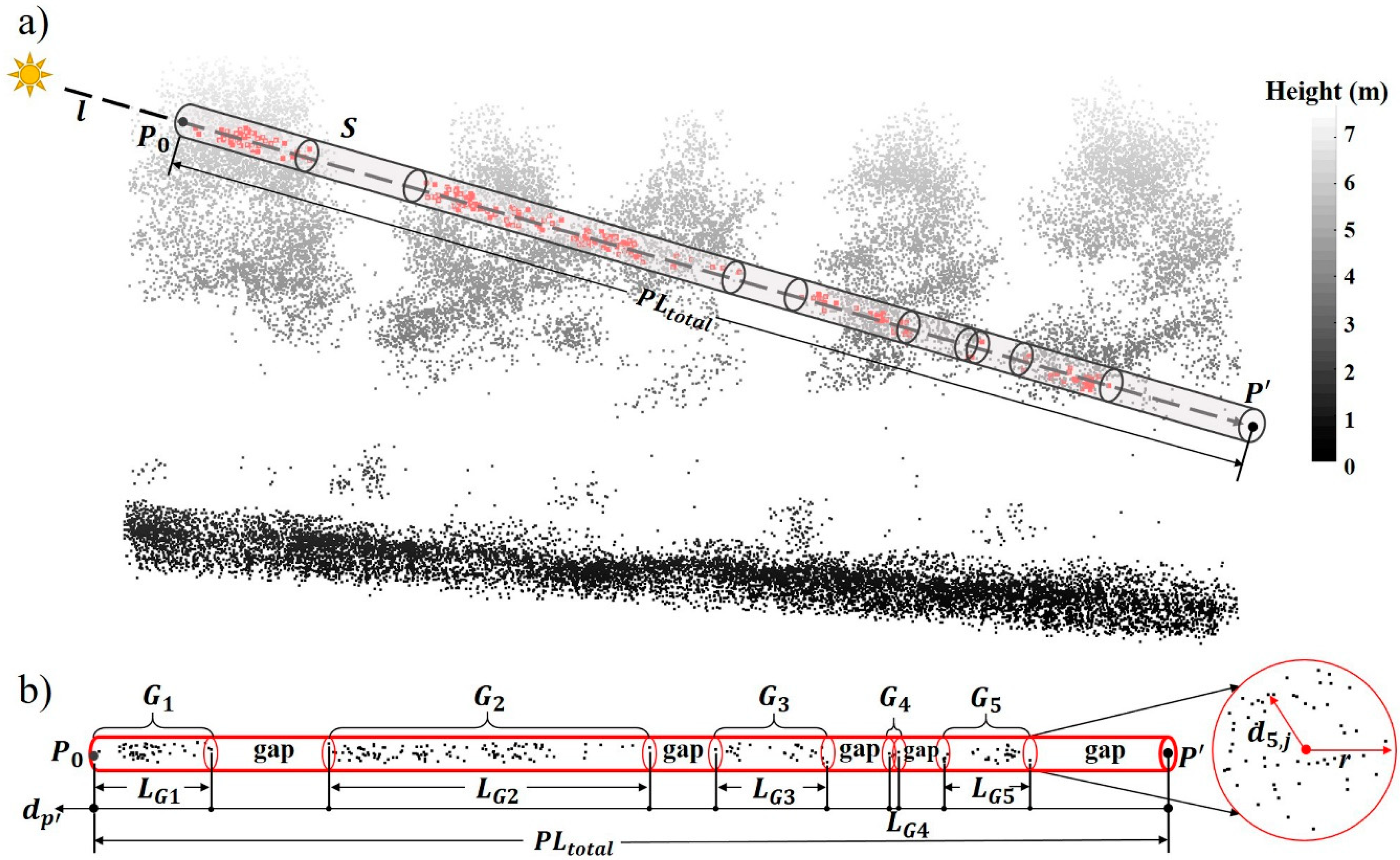
Figure 3.
The proportional contributions of sky radiance in each zenith-angle zone to the diffuse irradiance on a horizontal surface varied with solar zenith angle under a clear sky condition.
Figure 3.
The proportional contributions of sky radiance in each zenith-angle zone to the diffuse irradiance on a horizontal surface varied with solar zenith angle under a clear sky condition.
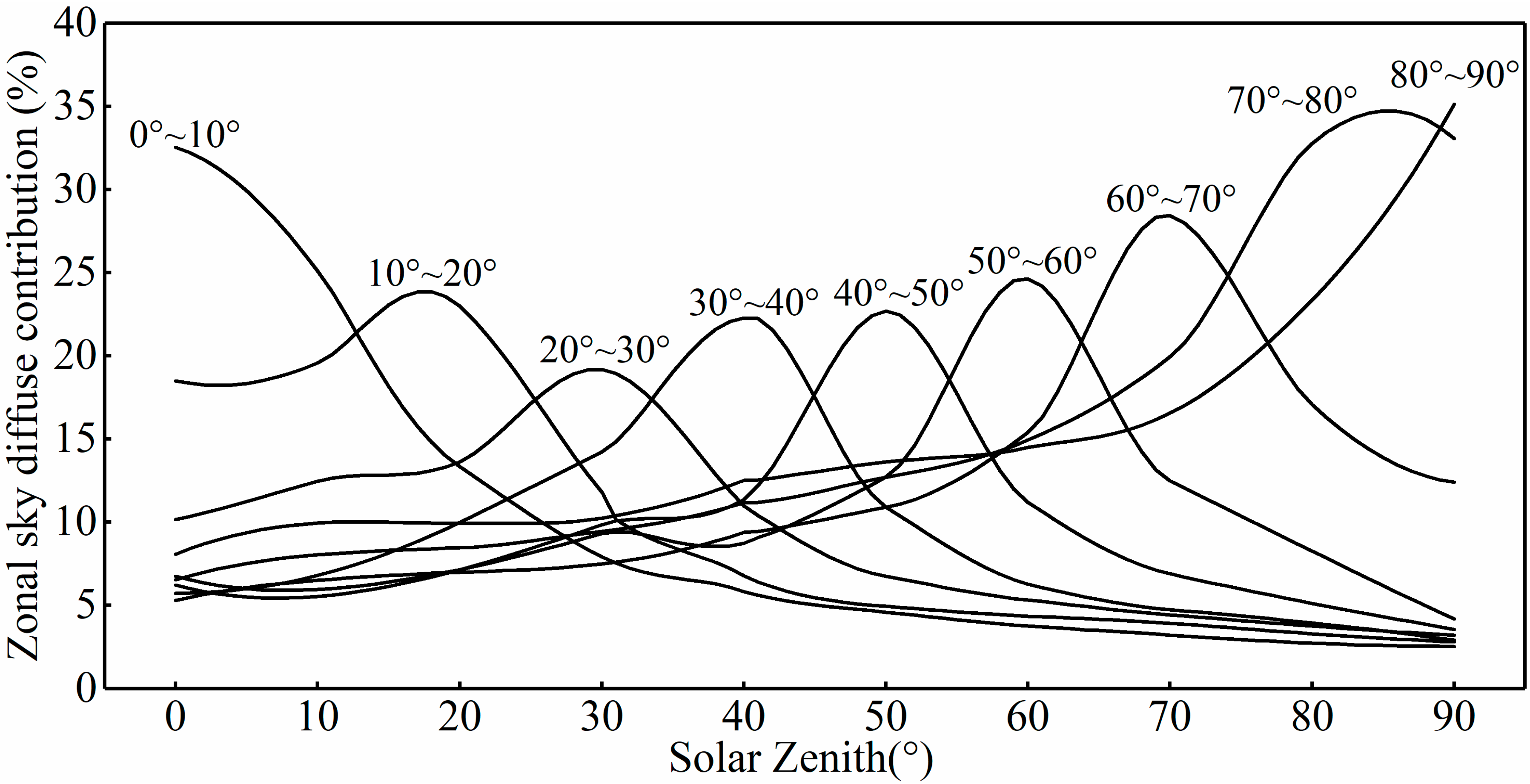
Figure 4.
The stereographic projection for lidar data. (a) The projected points of UAV lidar point cloud centered at the No. 5 observation location with a radius of 30 m. (b) The synthetic image derived from the TLS point cloud at the same location. The circle with a unit radius and the synthetic image were divided into 9 annulus rings for comparison.

Figure 5.
Fitting results of direct light attenuation model with three path length-based parameters calculated at two calibration locations. (a) The residual sum of squares and adjusted of fitting the direct light attenuation model with , and calculated with various r. (b) Scatter plot of direct PAR transmittance and calculated with optimal r. The red line indicates the fitting equation.

Figure 6.
Angular gap fraction at nine observation locations estimated with NPDs varying from origin to 25 cm and corresponding optimal parameters (Table 2). Reference values based on TLS-derived synthetic images are also given. Reference values for SVF and are shown in the upper left and upper right corner of each panel respectively.

Figure 7.
Evaluation results of the canopy radiation model using three light path length-based parameters at seven verification locations. (a) Variations of the mean value of MAE and bias between modelled and measured PAR with varied spatial buffer radius. (b) Scatter plot of modelled (y) total PAR based on with 15cm of r and observed (x) total PAR. The red line indicates the fitting equation and thin-dotted line indicates the 1:1 line.

Figure 8.
Variation trends of estimated direct, diffuse, total PAR and observed total PAR at each observation locations during one daily solar course.
Figure 8.
Variation trends of estimated direct, diffuse, total PAR and observed total PAR at each observation locations during one daily solar course.
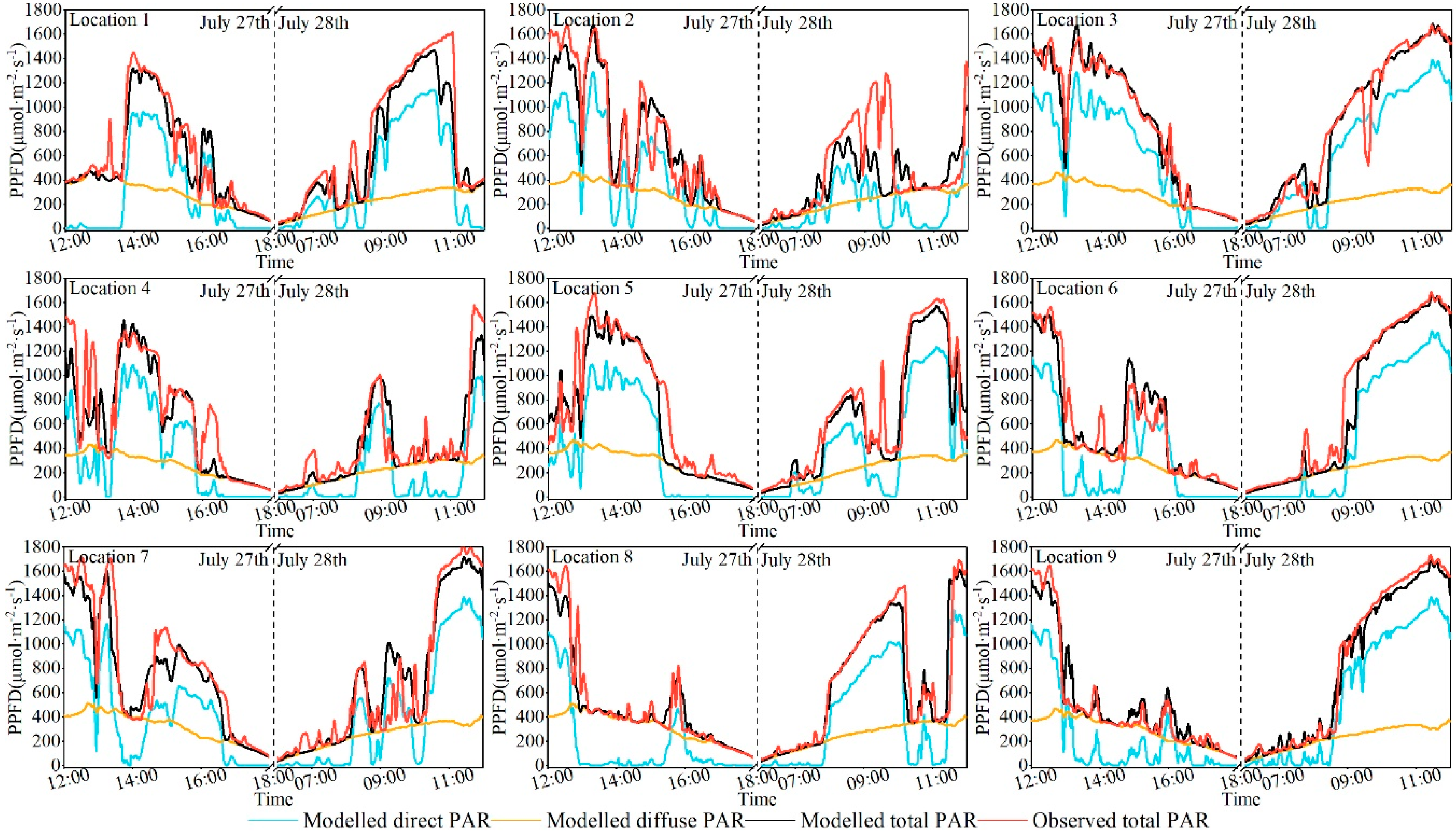
Figure 9.
Spatial patterns of total PAR in the forest floor at certain times during July 27~28, 2017 in the central part of the plot.
Figure 9.
Spatial patterns of total PAR in the forest floor at certain times during July 27~28, 2017 in the central part of the plot.

Figure 10.
Spatial patterns of total PAR along the vertical gradients (1, 3, 5, 6, and 7 m above the forest floor) at 12:00 on July 28, 2017 in the central part of the plot.
Figure 10.
Spatial patterns of total PAR along the vertical gradients (1, 3, 5, 6, and 7 m above the forest floor) at 12:00 on July 28, 2017 in the central part of the plot.
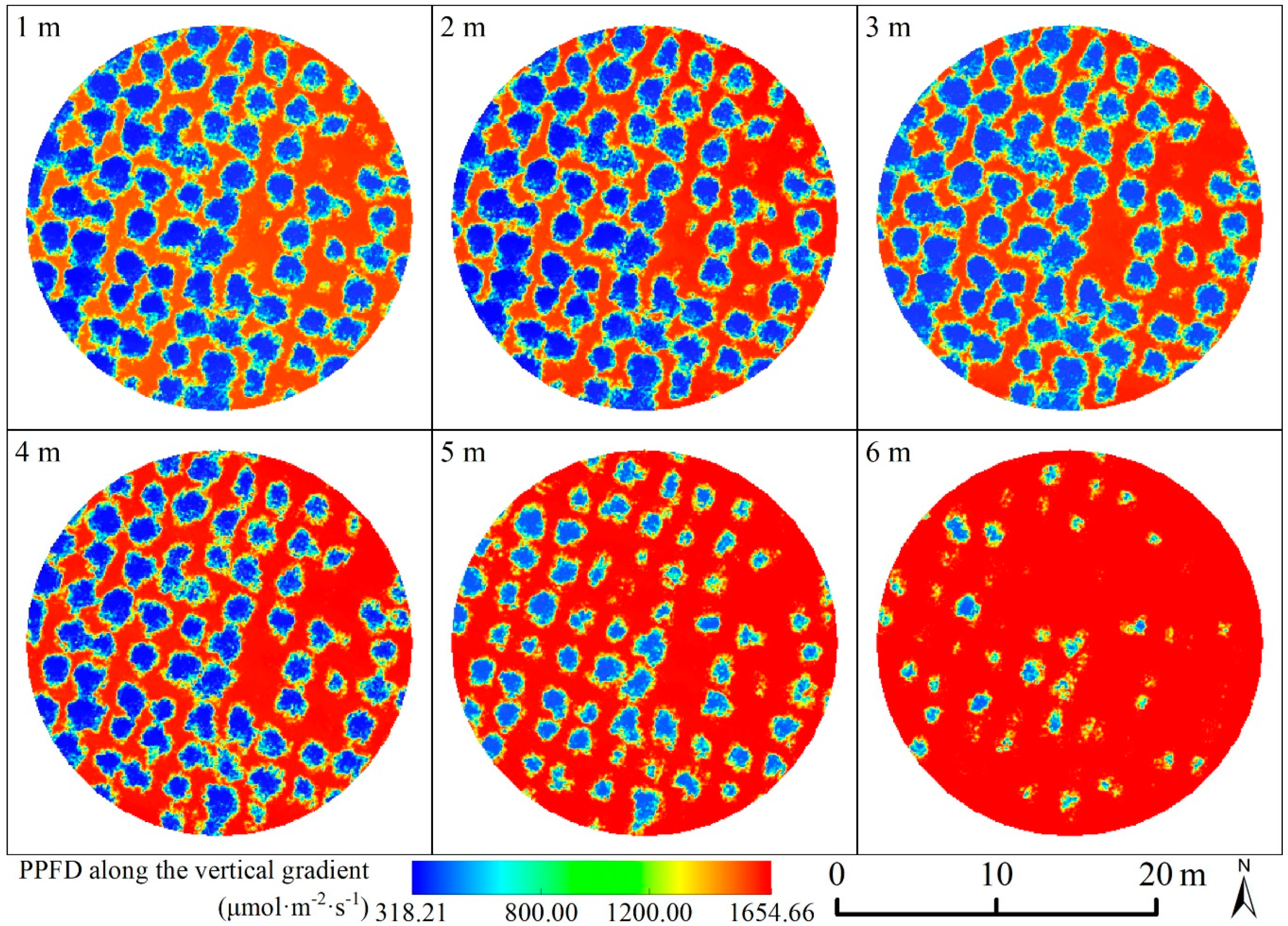
Figure 11.
The total PAR variations in the vertical profiles along the solar principal plane (SPP) and its perpendicular cross-plane (PCP) at certain times during July 27 ~ 28, 2017 in the central part of the plot.
Figure 11.
The total PAR variations in the vertical profiles along the solar principal plane (SPP) and its perpendicular cross-plane (PCP) at certain times during July 27 ~ 28, 2017 in the central part of the plot.

Figure 12.
Sensitivity analysis of three attenuation parameters for all observation locations at all recording times to the radius of spatial ray path buffer (r, in the 3D ray trace model). (a) Mean value and standard deviation of , and with varied r. (b)–(d) Percentage of , and values within their different value ranges with varied r. The solid square represents the zero value and the solid circle, triangle and diamond represent each value range.

Figure 13.
Path length-based parameters comparison: (a) and (b) changes of means and standard deviations of the difference between and or calculated with various spatial buffer radius (represented by different solid symbols) at exact same moments for all observation locations with . (c) variations of three path length-based parameters during a daily solar course at the No. 5 observation location with a spatial buffer radius of 15cm.

Figure 14.
Sensitivity analysis of parameters in the sky diffuse PAR model: (a) and (b) Changes of means and standard deviations of SVF and at 9 observation locations with R (original data with the optimal angle intervals given in Table 2 were used). (c) and (d) show changes of RMSE of estimated against reference values for each annulus ring with zenith and azimuth angle intervals, respectively. For a given zenith/azimuth angle interval, azimuth/zenith angle interval was optimized with R = 35 m.

Figure 15.
Comparison between isotropic and anisotropic sky diffuse distributions: (a) The normalized difference of and during a daily solar course. The red line and shading area indicate the mean value and the range of normalized difference at nine observation locations respectively. (b) The distribution of sky diffuse PAR arriving at the No. 5 observation location in each annulus ring at different moments under anisotropic sky diffuse distribution.

Figure 16.
The relationship between point density and model parameters. (a) The correlation coefficients of fitting the direct light attenuation model with calculated from data with various NPD levels varied with spatial buffer radius. (b) The distribution of in each annulus ring based on data with different NPD levels.


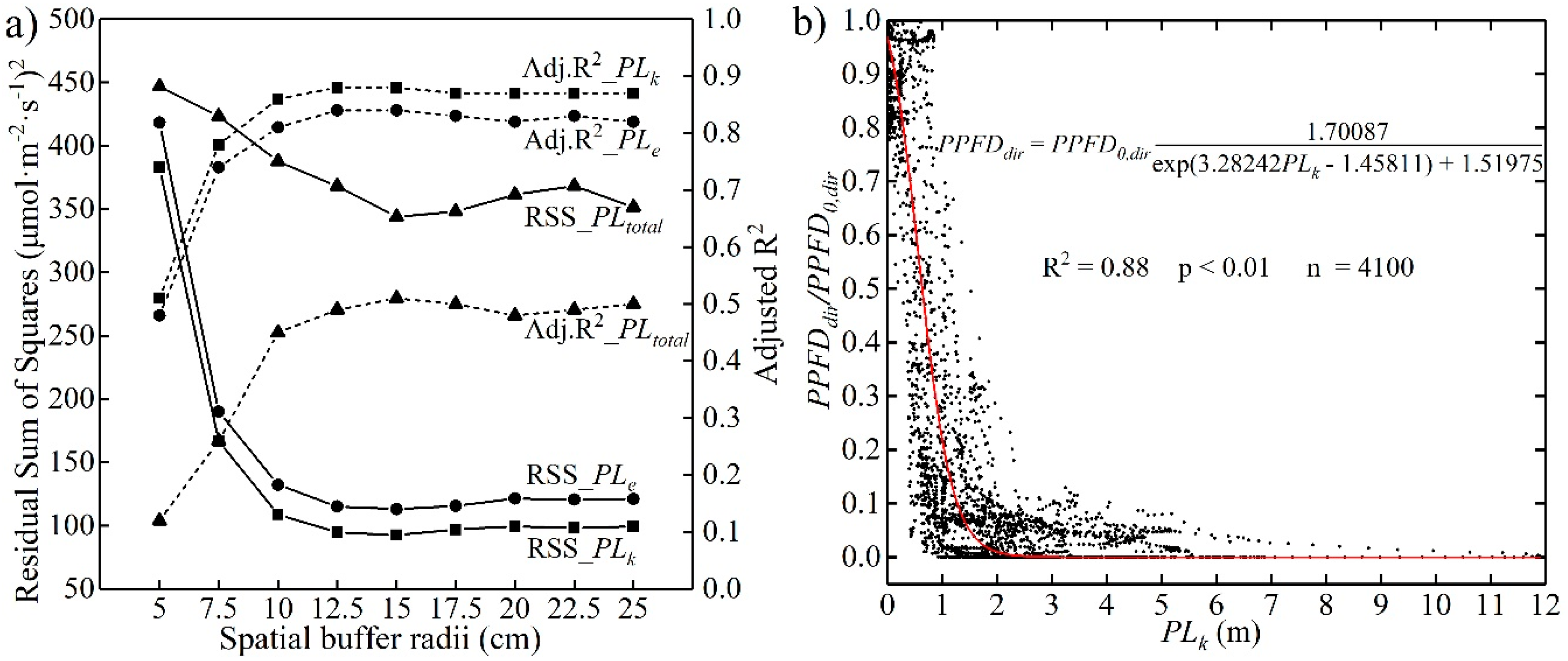
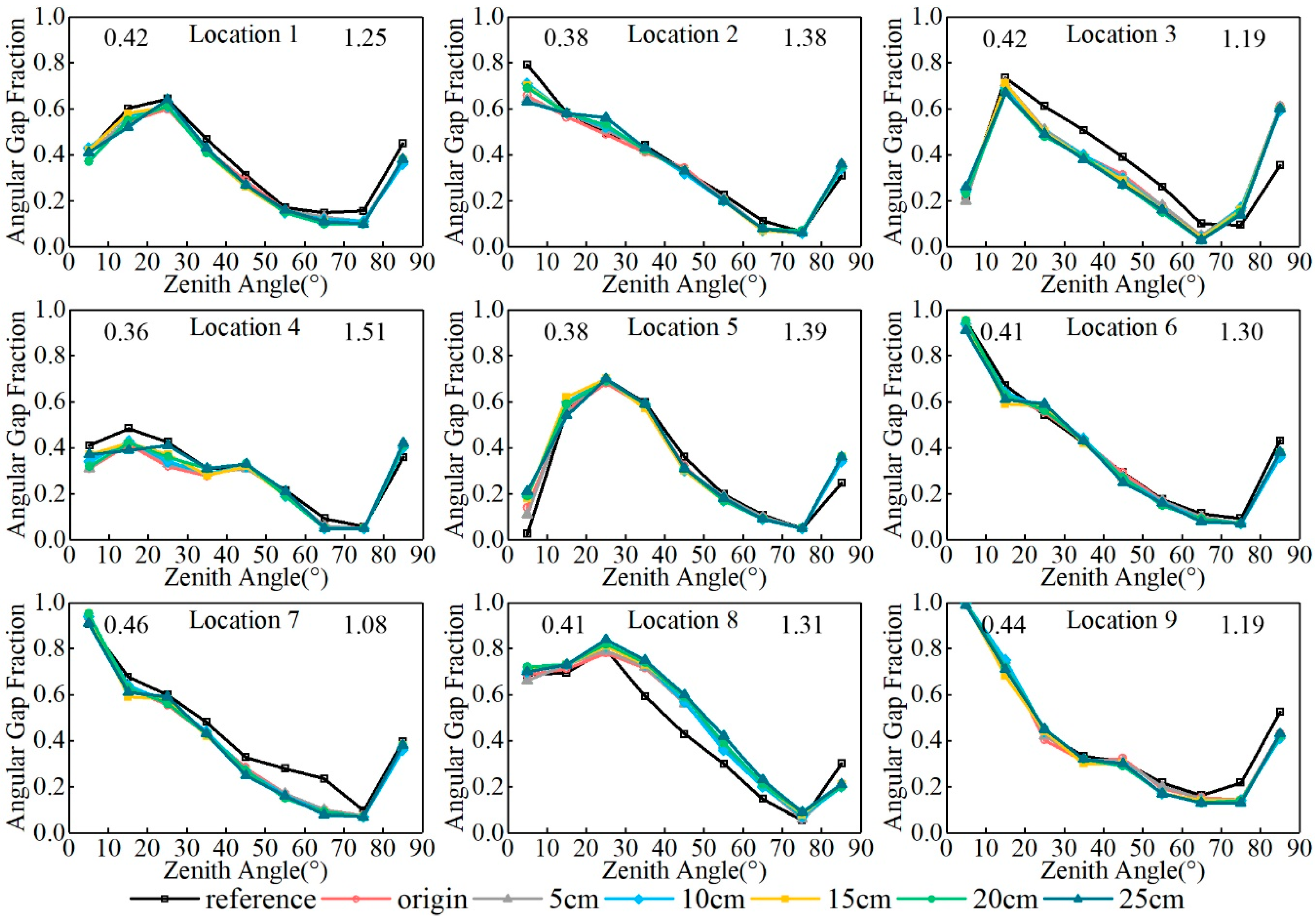
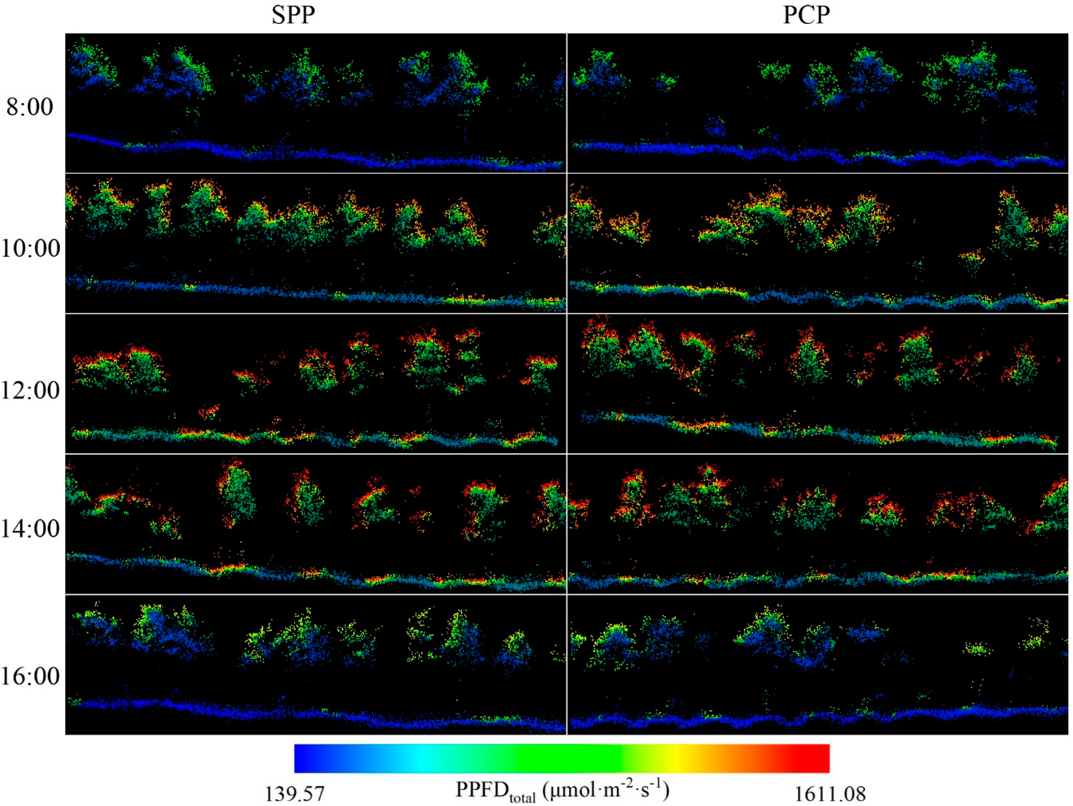
Table 1.
Locations of nine observation points in the experimental forest plot and calibration coefficients for each pyranometer at the corresponding location.
Table 1.
Locations of nine observation points in the experimental forest plot and calibration coefficients for each pyranometer at the corresponding location.
| Location Number | TLS Coordinates | ALS Coordinates | Height (m) | Calibration Coefficients | ||||
|---|---|---|---|---|---|---|---|---|
| X | Y | X | Y | a | b | c | ||
| 1 | −1.345 | −4.365 | 705589.46 | 3499268.53 | 0.36 | 0.60097 | 0.04742 | −0.000033 |
| 2 | −5.668 | −0.948 | 705584.46 | 3499266.03 | 0.21 | 0.51498 | 0.02754 | 0.000025 |
| 3 | 5.183 | 4.881 | 705584.29 | 3499278.50 | 0.33 | −1.30682 | −0.00527 | −0.000076 |
| 4 | −9.307 | 2.416 | 705579.89 | 3499264.47 | 0.32 | −0.59397 | −0.14066 | 0.000002 |
| 5 | −0.368 | 1.468 | 705584.65 | 3499271.91 | 0.75 | 1.00826 | −0.07162 | 0.000014 |
| 6 | −1.909 | −0.590 | 705586.14 | 3499269.84 | 0.12 | −1.19734 | −0.04765 | −0.000072 |
| 7 | 4.066 | −4.846 | 705592.75 | 3499273.31 | 0.38 | 6.77510 | 0.07835 | 0.000033 |
| 8 | 3.422 | 0.422 | 705587.54 | 3499275.07 | 0.73 | 0.24188 | 0.00924 | 0.000024 |
| 9 | −6.873 | −7.958 | 705590.59 | 3499261.92 | 0.11 | −0.63143 | −0.02538 | −0.000011 |
Table 2.
The optimal value of zenith angle interval () and azimuth angle interval () for calculating angular gap fraction () of first eight annular rings using data with different NPDs.
Table 2.
The optimal value of zenith angle interval () and azimuth angle interval () for calculating angular gap fraction () of first eight annular rings using data with different NPDs.
| NPD (cm) | 0°~10° | 10°~20° | 20°~30° | 30°~40° | 40°~50° | 50°~60° | 60°~70° | 70°~80° | ||||||||
|---|---|---|---|---|---|---|---|---|---|---|---|---|---|---|---|---|
| ∆θ1 | ∆φ1 | ∆θ2 | ∆φ2 | ∆θ3 | ∆φ3 | ∆θ4 | ∆φ4 | ∆θ5 | ∆φ5 | ∆θ6 | ∆φ6 | ∆θ7 | ∆φ7 | ∆θ8 | ∆φ8 | |
| (°) | (°) | (°) | (°) | (°) | (°) | (°) | (°) | |||||||||
| origin | 0.3 | 15 | 3 | 0.6 | 3 | 0.3 | 1 | 0.7 | 0.9 | 0.5 | 0.7 | 0.5 | 0.4 | 0.6 | 0.8 | 0.2 |
| 2.5 | 0.3 | 15 | 3 | 0.6 | 3 | 0.3 | 1 | 0.7 | 0.9 | 0.5 | 0.7 | 0.5 | 0.4 | 0.6 | 0.8 | 0.2 |
| 5 | 5 | 1 | 3 | 0.6 | 3 | 0.3 | 1 | 0.7 | 0.7 | 0.7 | 0.7 | 0.5 | 0.4 | 0.6 | 0.8 | 0.2 |
| 7.5 | 3 | 2 | 3 | 0.7 | 3 | 0.3 | 1 | 0.8 | 0.5 | 1 | 0.7 | 0.6 | 0.4 | 0.7 | 0.8 | 0.2 |
| 10 | 3 | 2 | 3 | 0.8 | 3 | 0.4 | 0.3 | 3 | 0.7 | 0.9 | 0.6 | 0.8 | 0.4 | 0.8 | 0.6 | 0.3 |
| 12.5 | 3 | 3 | 3 | 1 | 3 | 0.5 | 3 | 0.4 | 1 | 0.7 | 0.7 | 0.8 | 0.5 | 0.7 | 0.5 | 0.4 |
| 15 | 3 | 3 | 0.7 | 5 | 3 | 0.6 | 2 | 0.7 | 1 | 0.9 | 0.7 | 1 | 0.5 | 0.9 | 0.8 | 0.3 |
| 17.5 | 0.6 | 20 | 0.8 | 5 | 3 | 0.7 | 2 | 0.8 | 0.6 | 2 | 0.9 | 1 | 0.6 | 0.9 | 0.4 | 0.7 |
| 20 | 3 | 5 | 3 | 2 | 3 | 0.9 | 0.4 | 5 | 0.7 | 2 | 0.5 | 2 | 0.7 | 1 | 0.8 | 0.4 |
| 22.5 | 0.8 | 20 | 3 | 2 | 3 | 1 | 3 | 0.9 | 0.6 | 3 | 0.6 | 2 | 2 | 0.4 | 0.4 | 0.9 |
| 25 | 0.8 | 25 | 3 | 3 | 0.7 | 5 | 3 | 1 | 4 | 5 | 3 | 0.5 | 1 | 0.9 | 0.5 | 0.9 |
© 2019 by the authors. Licensee MDPI, Basel, Switzerland. This article is an open access article distributed under the terms and conditions of the Creative Commons Attribution (CC BY) license (http://creativecommons.org/licenses/by/4.0/).
Share and Cite
MDPI and ACS Style
Zeng, K.; Zheng, G.; Ma, L.; Ju, W.; Pang, Y. Modelling Three-Dimensional Spatiotemporal Distributions of Forest Photosynthetically Active Radiation Using UAV-Based Lidar Data. Remote Sens. 2019, 11, 2806. https://doi.org/10.3390/rs11232806
AMA Style
Zeng K, Zheng G, Ma L, Ju W, Pang Y. Modelling Three-Dimensional Spatiotemporal Distributions of Forest Photosynthetically Active Radiation Using UAV-Based Lidar Data. Remote Sensing. 2019; 11(23):2806. https://doi.org/10.3390/rs11232806
Chicago/Turabian StyleZeng, Kuo, Guang Zheng, Lixia Ma, Weimin Ju, and Yong Pang. 2019. "Modelling Three-Dimensional Spatiotemporal Distributions of Forest Photosynthetically Active Radiation Using UAV-Based Lidar Data" Remote Sensing 11, no. 23: 2806. https://doi.org/10.3390/rs11232806
Note that from the first issue of 2016, this journal uses article numbers instead of page numbers. See further details here.