Article

A Proposed Methodology to Analyze Plant Growth and Movement from Phenomics Data

by
María Victoria Díaz-Galián
1,
Fernando Perez-Sanz
2,
Jose David Sanchez-Pagán
3,
Julia Weiss
1,
Marcos Egea-Cortines
1 and
Pedro J. Navarro
4,*
1
Genética Molecular, Instituto de Biotecnología Vegetal, Edificio I+D+I, Plaza del Hospital s/n, Universidad Politécnica de Cartagena, 30202 Cartagena, Spain
2
Biomedical Informatic and Bioinformatic Platform, Biomedical Research Institute of Murcia, University Clinical Hospital ‘Virgen de la Arrixaca’, University of Murcia, 30120 Murcia, Spain
3
Ecología y Nuevas Tecnologías, Avda. Lorca 193, 30835, Sangonera la Seca, 30120 Murcia, Spain
4
Escuela Técnica Superior de Ingeniería de Telecomunicación (DSIE), Campus Muralla del Mar, s/n, Universidad Politécnica de Cartagena, 30202 Cartagena, Spain
*
Author to whom correspondence should be addressed.
Remote Sens. 2019, 11(23), 2839; https://doi.org/10.3390/rs11232839
Submission received: 14 October 2019 / Revised: 18 November 2019 / Accepted: 25 November 2019 / Published: 29 November 2019
(This article belongs to the Special Issue Advanced Imaging for Plant Phenotyping)

Abstract

:
Image analysis of developmental processes in plants reveals both growth and organ movement. This study proposes a methodology to study growth and movement. It includes the standard acquisition of internal and external reference points and coordinates, coordinates transformation, curve fitting and the corresponding statistical analysis. Several species with different growth habits were used including Antirrhinum majus, A. linkianum, Petunia x hybrida and Fragaria x ananassa. Complex growth patterns, including gated growth, could be identified using a generalized additive model. Movement, and in some cases, growth, could not be adjusted to curves due to drastic changes in position. The area under the curve was useful in order to identify the initial stage of growth of an organ, and its growth rate. Organs displayed either continuous movements during the day with gated day/night periods of maxima, or sharp changes in position coinciding with day/night shifts. The movement was dependent on light in petunia and independent in F. ananassa. Petunia showed organ movement in both growing and fully-grown organs, while A. majus and F. ananassa showed both leaf and flower movement patterns linked to growth. The results indicate that different mathematical fits may help quantify growth rate, growth duration and gating. While organ movement may complicate image and data analysis, it may be a surrogate method to determine organ growth potential.

Graphical Abstract

1. Introduction

The study of plant movement has a long tradition with observations of various plant species performed already in the nineteenth century by Darwin and others [1,2]. Plant movement and growth can show diel patterns as a result of coordination by the plant’s circadian clock and environmental cues such as light and temperature. The circadian clock is comprised of a set of genes that coordinate environmental inputs into the genetic control of biological processes. The interaction between the clock and the environment produces several outputs and is a general mechanism found in plants to anticipate daily changes in the environment, such as dusk and dawn [3]. The outputs of the circadian clock occur at discrete periods of the day giving rise to the concept of gated responses [4]. The plant circadian clock is coordinated with the environment via light and temperature signaling [5,6,7,8]. However, not every gated phenotype is due to the circadian clock [9], as they might depend directly on photoperiod or thermoperiod, and fade away under free-running conditions of continuous light, dark or temperature.
Plant growth is one of the main traits for plant improvement, as it is related to yield. Growth has been dissected into growth speed and growth duration in a variety of model systems and crops [10,11,12]. In principle, the growth rate should be identified by adjusting a mathematical function to a set of data taken over time. The basic functional forms of growth described for plants include linear growth, non-linear non-asymptotic growth and non-linear asymptotic exponential growth [13]. When analyzed with enough resolution, sometimes growth is not linear for a 24 h period and shows a gated pattern. Gated growth patterns may be circadian, with growth patterns adjusting to a 24 h period or ultradian with several cycles found in a day. The growth rate shows a circadian gating in Arabidopsis hypocotyls and leaf disks of tobacco grown in vitro [14,15]. As growth is not always linear when analyzed with sufficient time resolution, linear models do not always produce the desired fit. Yet an additional issue when analyzing plant growth by image and time-lapse analysis is plant movement.
There are two general types of plant movement, organ movement and shoot movement, also known as circumnutation. Originally described by Darwin, circumnutation is found in a variety of plants, such as Arabidopsis, Helianthus or rice to name a few [16,17,18]. There are several types of organ movement, including stem circumnutation or leaf movement. Stem circumnutation is ultradian in beans while leaves show a circadian movement [19]. Circadian leaf movement was originally detected in beans [20]. Circadian leaf movement has been described in tomato, Arabidopsis, bean or Pharbitis to name a few [20,21,22,23]. Like other biological processes, determining if a gated behavior is driven by an endogenous clock or by external signals such as light is studied by performing free-running conditions of continuous light or dark [24].
A powerful method to obtain phenotypic data is through image acquisition. Image-based phenomic technologies have triggered a change in how experiments are carried out [25]. The main advantages are the low costs, non-invasive techniques and the possibility of obtaining quantitative data, such as in research about circadian clocks, growth analysis, the detection of pathogen attack or oxidative stress [26,27]. There are several methods of acquiring images that differ on the type of camera used, including 2D, 3D, monochromatic, multispectral and hyperspectral cameras [28]. Data acquisition from images is a complex process starting with image preprocessing, segmentation, feature extraction and classification [29]. As a result, the combination of background, incident light and acquisition wavelength are three components of image analysis.
Two major trends are found in image-based phenomics. One is the image acquisition of open space and large plant fields to monitor parameters such as growth, senescence, abiotic or biotic stresses [30,31]. A second one is based on experiments in confined environments and controlled conditions. Many experiments using transgenic material are performed in greenhouses or growth chambers as open field conditions are subject to strong local legislation and are sometimes forbidden. There is a long-standing tradition in plant genetic models, such as Arabidopsis, Tobacco, Petunia or snapdragon. Studies using the LUCIFERASE reporter genes in Arabidopsis and image acquisition paved the way to identify mutations in highly complex processes, such as circadian clock [32] or abiotic stress responses [33]. Further studies have used tobacco [14], petunia [10], tomato [21] or snapdragon [34] to identify diel growth patterns or the effect of gene knockdowns on growth. Both field and confined image-based phenomics share a common set of tools and solutions to acquire and process images.
In this work, the methodology to analyze raw data obtained from images in plants, taking into account growth and movement, is explored. Growth and movement were analyzed in the Antirrhinum majus, A. linkianum, Petunia x hybrida and Fragaria x ananassa species. These species were selected because they have different growth habits. Obtaining quantitative data requires a set of mathematical tools that depend on the growth curve, and depending on the data set, linear, exponential, logarithmic, polynomial or generalized additive models (GAM) may give best fits. Finally, it was observed that although movement may complicate direct growth measurement, it can be a surrogate phenotypic trait related to growth potential.

2. Materials and Methods

2.1. Plant Material and Growth Conditions

Four different species were used with different growth habits. The Antirrhinum species A. majus and A. linkianum have a classic spike inflorescence but differ in the erect habit of A. majus and trailing growth habit of A. linkianum [35]. Petunia x hybrida is a Solanaceae close to tomato with a sympodial inflorescence [36,37]. The cultivated strawberry Fragaria x ananassa has a rosette growth habit and produces inflorescences in stolons [38].
The inbred line from Antirrhinum majus 165E and the wild species A. linkianum [35,39] were used. Petunia experiments were performed with the double haploid Petunia x hybrida W115 Mitchell [40]. Seeds of Antirrhinum and Petunia were germinated under a day/night cycle of 12:12 LD and 23 °C 18 °C in vermiculite. Plants were kept at 100% humidity in the soil and 60%–70% in the growth chamber (Table 1).
Commercial strawberries Fragaria x ananassa cv. Fortuna, were obtained from a local company and grown in a growth chamber. We measured six stems (A–F) differing in their developmental stage. A was the oldest while F was the youngest. The thermoperiod was of 23–8 °C coupled to a photoperiod of 16 h light and 8 h dark (Table 1). Illumination was performed using a custom-made LED comprising 8 channels of 395 nm (ultraviolet), 450 and 470 nm (blue), 528 nm (green), 620, 660 and 730 nm (red) 820 (infrared). The average power was 90 Watts and the light angle 110° [41]. Experiments were also conducted under continuous light and continuous dark conditions. Between continuous light or continuous dark periods, one long-day photoperiod was given to identify effects on growth and movement. A third experimental setup consisted of changing wavelength quantities of the amount of blue and red light. Standard rates were identical powers for all wavelengths and modified rates included 1:7 (Blue/Red) or low rate B/R and 3:7 B/R, or high rate B/R, while other wavelengths were kept at 1. The photosynthetic active radiation ranged between 71.69 and 118.65 µM/s/m2.

2.2. Image Acquisition

Plants were grown inside a configurable growth chamber equipped with a camera for image acquisition and a home-made system to control light/dark periods and light activation previously described [42]. The software controlling image acquisition and light conditions allows obtaining images at required times. Images were taken at ten- to sixty-minute intervals activating an infrared LED in order to avoid modification of the circadian clock [43]. A file was automatically created by the program. This text file included metadata such as the specific time, the name of the image and all the parameters about the vision system and lighting.

2.3. Image Analysis

Images were manually marked for further analysis. A set of points were selected in each experiment to get their coordinates. Once reference points were selected, all these points had to be manually tracked for all the images studied. Thus, each image was a sample that was marked, as many times as the reference points that had been chosen, in order to obtain the coordinates of each reference point and, consequently, to transform them into distances.
The use of the internal coordinates allowed the conversion of the measurements from coordinates into data in mm. The organ length was determined by placing two reference points at the beginning and the end of an organ. Comparing a series of images allowed the identification of growth rate. The organ movement was determined by superposing a set of images and identifying the distance covered by the plant organ for a given period of time.
Image analysis was performed in R version 3.5.3 using the image processing libraries “imager” and “bmp”. Data visualization was done with the library “ggplot2”, which allowed the creation of the graphics. Library “imager” is an image processing library designed to work with image data, filtering, morphology and transformations. The “bmp” package allows reading Windows bitmap (BMP) images. Both libraries, “imager” and “bmp” were used in order to work with the images acquired with the vision system. The “readr” package allows the ability to read many types of rectangular data, including csv, tsv and fixed-width files and it was necessary to open the files where the obtained data (coordinates, lengths or any other information) were stored. Another package applied was “boot”, which provides extensive facilities for bootstrapping and related resampling methods. The “mgcv” package was used for generalized additive modeling, including generalized additive mixed models.
Data were analyzed for rhythmic patterns with the MetaCycle package [44], using the implemented algorithms of ARSER, JTK_Cycle and Lomb–Scargle [45]. MetaCycle package detects rhythmic signals from time-series datasets. Linear, exponential, logarithmic, polynomial and GAM trend lines were obtained using built-in commands in R. The area under the curve (AUC) was analyzed with the “DescTools” library, which allows the ability to calculate descriptive statistics, draw graphical summaries and report the results. In this study, it was used for the obtention of AUC in leaf stem of Strawberry.

2.4. Statistical Analysis

Several statistical tests were done in order to acquire more information from the images. Once organ lengths were obtained for a period of time, trend lines were fitted to identify the best adjustment. Linear, exponential, logarithmic, polynomial and GAM trend lines were tested. In the case of the polynomial trend line, it was necessary to do the elbow method [46] before selecting the appropriate number of parameters for this analysis (Table 2). The maximum slope of the fitted curves was obtained with a custom R script that calculated the first derivative.
The MetaCycle package has three different algorithms. We selected JTK-Cycle, a non-parametric statistical algorithm designed to identify and characterize cycling variables in large datasets [45]. This algorithm gives five outputs: Benjamini–Hochberg critical value (BH.Q), adjusted p-value (ADJ.P) period, amplitude and LAG. Significant rhythms were tested using the Benjamini–Hochberg critical value (BH.Q), Q, controlling the false discovery rate. Adjusted p-value (ADJ.P) is used as a cut-off to identify clock-regulated transcripts. When both of them are less than 0.05, a circadian rhythm is accepted. The period is the time covered by a cycle. LAG is the time of the first peak from subjective time 0, the moment lights are turned on. Amplitude is half of the size of a wave. Period and LAG are expressed in hours, while the rest of the parameters are dimensionless.
The area under the curve gives a mathematical value corresponding to the development of the organ size. Mathematically, it represents the integrate of the organ length (leaf petiole) of Strawberry throughout time. The higher this value is, the bigger the organ was at the beginning of the experiment or the faster the organ grew. The unit is cm × h.

3. Results

3.1. Acquisition of Coordinates and Calibration

In order to obtain data on growth and movement, a set of internal and external coordinates need to be defined. While analyzing growth using a single internal point mathematically defined, such as the center of gravity, is a proven method [42], it is simpler to use two internal coordinates for growth. Visual inspection of a time-lapse video made out of the images of a given experiment will aid in determining the exact points giving higher accuracy. Based on these criteria, different internal coordinates were taken depending on the specific features of the plant and image. When images were taken in a zenithal view (top view), it was possible to study both growth and leaf movement at early stages of growth. Images can also be acquired with a front view, and with this orientation it is possible to obtain leaf movement, and sometimes its angle, without losing information on growth. Front view images present an issue because parts of the plant can hide the selected points. Furthermore, the selected parts can modify their angle with respect to the camera. The most adequate moment to measure leaf length with precision is when they show a straight or nearly straight line in one axis. Considering that leaves do not shrink under our growth conditions, a decrease in size reflects a change in position due to movement.
Growth of Antirrhinum linkianum and A. majus seedlings was analyzed (Video S1). Three points of each seedling were selected for our study: the center of the seedling and the edge of each leaf. The edge of the pot was used as internal coordinates for analysis (Figure 1a). With this selection, seedling movement and leaf growth could be analyzed using a zenithal view (Figure 1a, Video S1).
The Petunia plant was analyzed using a front view selecting four points for each leaf: The insertion point of stalk in the petiole; the end of petiole; half of leaf; and end of leaf (Figure 1b). A picking tag was used as internal coordinates. A point in the middle of each leaf was selected because a strong leaf movement was observed (Figure 1b, Video S2) and, otherwise it would have been impossible to obtain accurate measurements of leaf growth or movement.
Fragaria x ananassa was studied using a front view. Here we focused on how leaves grew and moved. Taking into consideration how the plant grows (Figure 1c, Video S3), three reference points were selected for each leaf: the crown, middle of petiole and end of petiole (Figure 1c). With these three points, most issues caused by the leaf movement were avoided as stalks were not always straight. The edge of the pot was again used for internal coordinates.

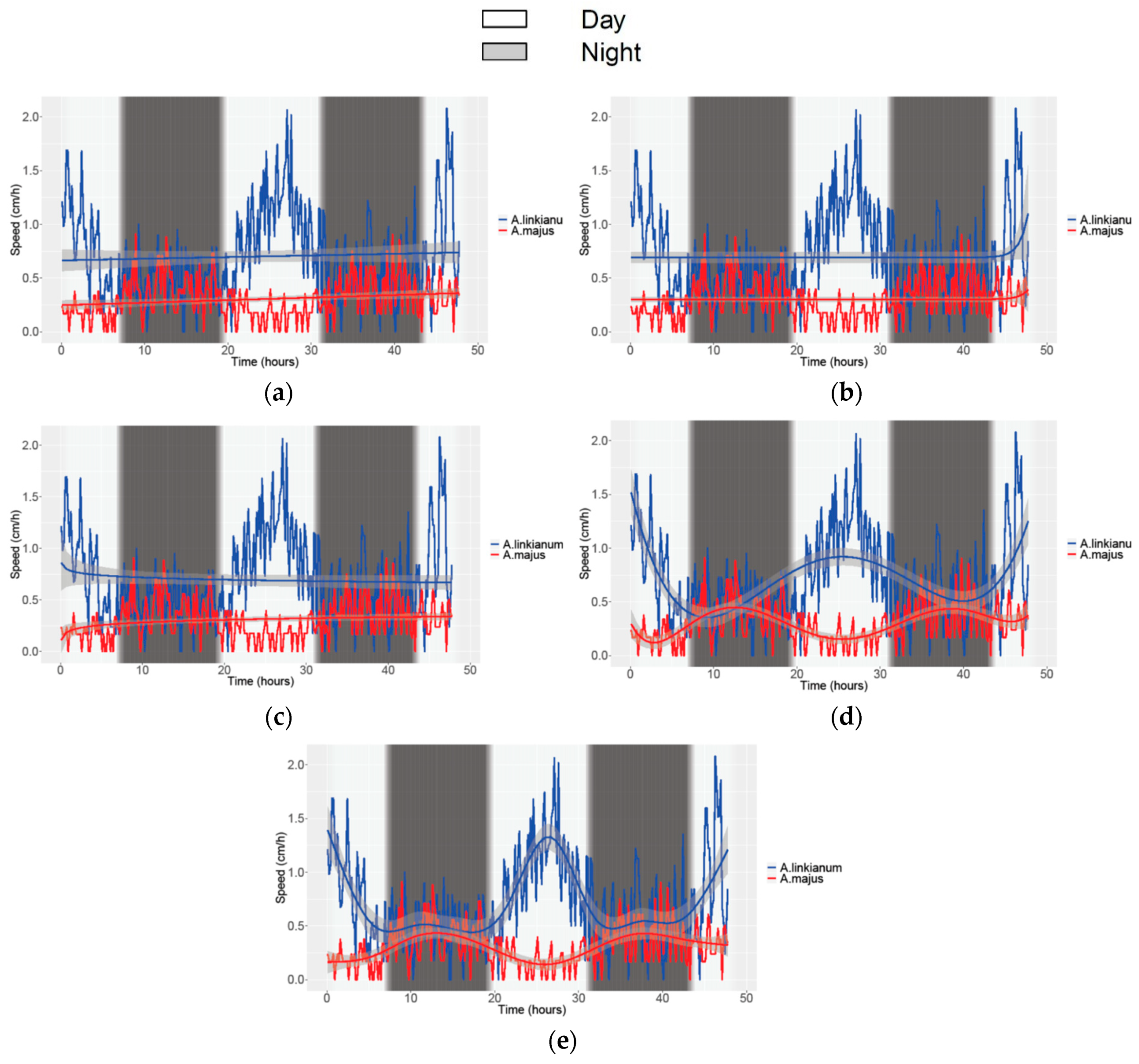
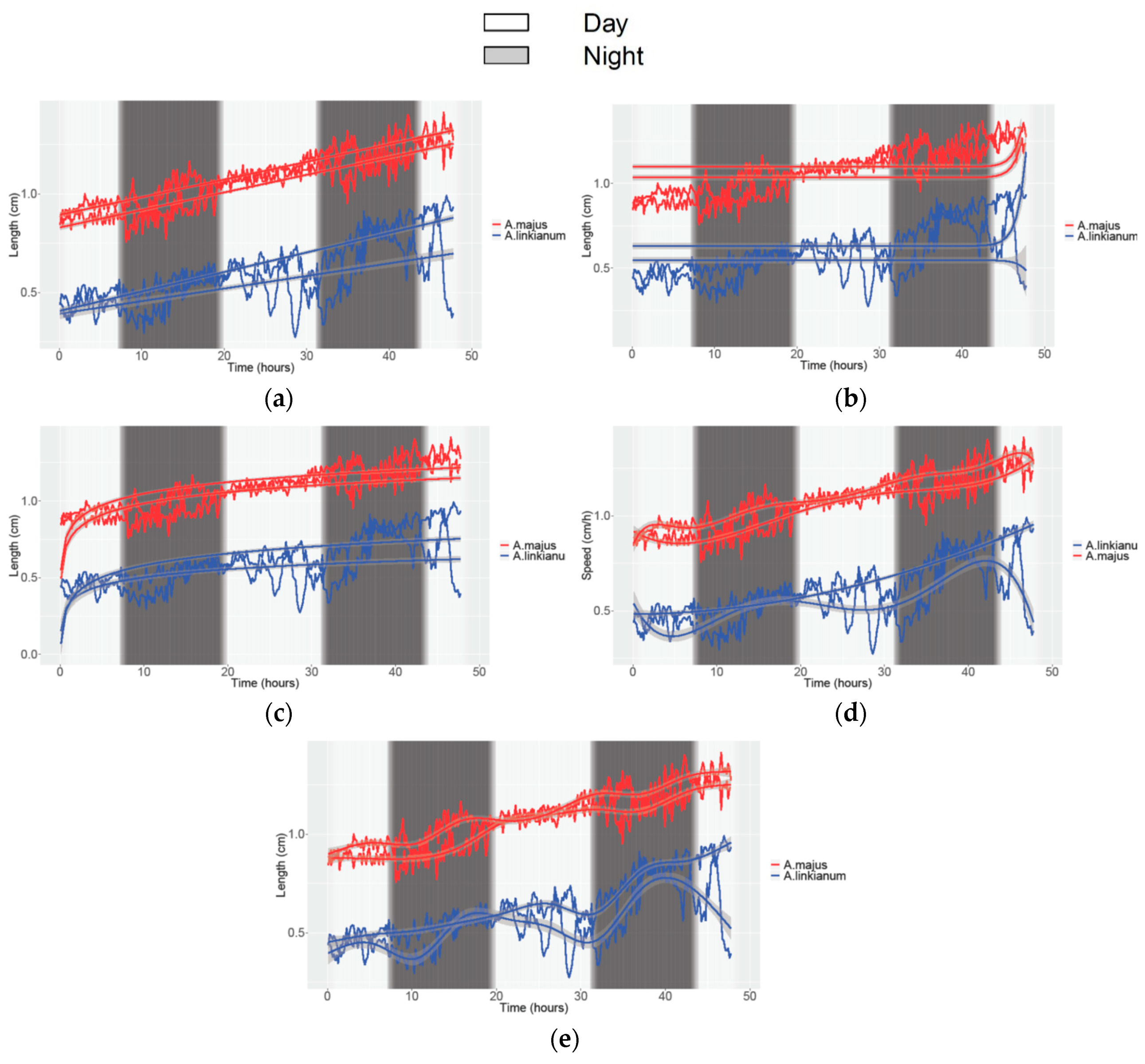
3.2. Obtaining Data of Growth and Movement in Antirrhinum

Speed movement of A. linkianum vs A. majus was analyzed studying the reference points placed in the center of the seedling (Figure 1a, Video S1) (Table 1). Using top view, movement was studied taking as reference the center of the seedling. Movement speed was calculated using the different positions taken by the center of the seedling throughout the time or images (Video S1). In addition, five trend lines were plotted in order to identify the best fit (Figure 2a–e).
Linear, exponential and logarithmic trend lines were overall unsuitable, due to poor fitting with the raw data. GAM (Figure 2e) gave better data fitting. The curve adjustments were very low for linear, exponential and logarithmic curves (Table 3), as their R2 coefficients of determination had a value around zero. Both polynomial and GAM trend line had almost the same value (Table 3). Indeed, their fitting to the data was similar (Figure 2d–e). However, the A. majus behavior in both trend lines was different and it fits best with the GAM equation (Figure 2d–e and Table 3). Although the polynomial fitting gave a good trend line, the GAM fitting was more precise, especially during the night period (Figure 2e).
The data analysis showed that there is a major difference in speed of movement in A. majus and A. linkianum during the day, but they show a similar movement speed during the night. Furthermore, they appeared to have opposite movement phases as A. majus displayed the maxima at night and A. linkianum during the day. Based on the GAM fit, speed of A. linkianum was up to 1.5 cm/h while the fastest speed recorded for A. majus was less than 0.5 cm/h.
Growth of A. majus and A. linkianum leaves was further analyzed (Figure 3a–e). Leaf length was obtained with the distance between each center of the seedling and the edge of each leaf. We measured two leaves, thus obtaining two R2 for each species. Although the linear equation showed low coefficient of determination values (Table 3), it was a good estimator for average growth speed over long time periods (Figure 3a and Table 3). Inspecting the linear fit curves, growth rate appeared to be similar in both species with an approximate growth speed of 4 mm/day. However, when the GAM fits were inspected, growth appeared to occur at higher speed at the end of the subjective night in both species (Figure 3e), indicating a gated growth pattern. It can be concluded that in some experiments, different types of curve fits allow the obtention of data about growth rate and growth gating. Thus, a single curve fit may not be enough to obtain all the information that can be obtained from a single set of experiments (Figure 3 and Table 3).

3.3. Obtaining Data of Movement and Speed in Petunia

Plant movement has been used as a surrogate to identify genetic variants in the circadian clock in tomato [21]. Petunia x hybrida, a Solanaceae related to tomato [37], was used, with a focus on fully grown leaves as movement was easier to observe (Table 1). The movement was studied with the angle found between the end of the leaf petiole and the middle of the leaf (Video S2). The plant was exposed to several photoperiods: 12/12 h light/dark (Figure 4a); 24 h light (Figure 4d); 24 h dark (Figure 4g). Under 12/12 LD photoperiodic conditions, leaves showed a strong movement pattern (Figure 4a), but movement appeared to be lost when plants were grown under free-running conditions of continuous light or continuous dark (Figure 4d,g). However, a closer inspection of the fitted curves indicated a residual movement in continuous light (see below). It is worth noting that leaf angle was kept as the light angle under continuous light and dark angle under continuous dark.
Inspecting all trend lines for each photoperiod (Figure 4 and Figure S1), the best fit was achieved with GAM. However, the polynomial trend line (Figure 4h) gave the best fit for movement during continuous darkness (Figure 4g–i and Figure S1g,h), as the polynomial trend line showed the highest R2 (Table 4), even though it is similar to that obtained with GAM lines. Regardless of the importance of knowing which trend line gives the best fit, the raw data are highly relevant in this case in order to inspect plant movement during dark/light transitions. This is due to the smoothness in the trend lines, which removes important information about leaf movement. The raw data show how sudden organ position changes occur. As square waves of leaf movement were found, this information was considered more relevant than any of the fits found with the different mathematical approaches.
The same experiment of Petunia was processed focusing on the transition between photoperiods in order to identify how fast the plant was able to adapt itself to the new environmental conditions (Figure 5 and Figure S2). In all cases, the raw data was more informative than the fitted trend lines. As previously seen, organ angle followed a squared function with very rapid change after transition to light or dark periods (Figure 5). The only experimental data that showed a good fit was the transition from continuous dark to 12/12 h light/dark, as well as 12/12 h l/d to continuous light (Table 5). These trend lines are highly accurate (Table 5) (Figure 5d,f). In contrast, the transition between continuous light and 12/12 h L/D showed poor fit because adaptation is very fast and the points were considered as outliers by the algorithm (Figure 5 h). From the raw data inspection we can see that after a period of continuous dark, leaf angle recovered immediately to a light angle (Figure 5e), while it took 24 h to recover when exposed to continuous light (Figure 5g).
As leaf movement showed a square wave appearance (Figure 4 and Figure S1), which seems to be rhythmic, with day–night changes, adjustments to circadian cycles were tested. Indeed, for a 12/12 L/D photoperiod, leaves displayed a significant rhythm of 24–25 h (Table 6). Leaf rhythmic movement was lost under continuous light or dark indicating that it was driven by light signaling and not via the circadian clock. While the rhythm had been lost, the period was maintained in continuous light and became shorter by roughly four hours in continuous dark. Finally, both running conditions caused a drastic decrease in movement amplitude.
Movement speed of the leaf was calculated as the difference of position of the end of the leaf throughout the time i.e., the distance of a point between two images. As the movement speed is steep, none of the trend lines showed an adequate fit to the data (Figure 6, Figure S3 and Table 7). As trend lines algorithms assume that the peaks (Figure 6) are outliers, it is impossible to see them on their trend lines. Speed was up to 3 cm/h during 12/12 L/D photoperiods but decreased sharply under continuous light and disappeared under continuous dark indicating a rapid effect on leaf movement through lighting.
Movement speed was analyzed for circadian cycling. There was a big difference in speed and movement amplitude between leaf 1 and 2 but both showed a significant rhythm under LD conditions (Figure 6a and Table 8). Under free-running conditions of LL or DD, the observed rhythms were lost indicating that leaf movement in Petunia is completely dependent of photoperiod. During 12/12 h L/D, leaf 1 showed a 12 h period for speed corresponding to two movements, while leaf 2 showed a 24 h period, owing to its position (Video S2). The daily change in angle was knocked down to a single change during 24 h light and 24 h dark. The lag phase was modified between 1.5 and all the way to 17 h (Table 8). Finally, and as seen before for movement, the amplitude was reduced by free-running conditions. Altogether it can be concluded that leaf movement in petunia is not circadian regulated but dependent on photoperiod.

3.4. Analyzing Growth and Movement in Strawberry

Finally, the growth of strawberry and its movement was studied after being subjected to four photoperiods in order to identify if there was a link between photoperiod and plant growth (Video S3). Illumination was performed using a custom-made LED comprising 8 channels of 395 nm (ultraviolet), 450 and 470 nm (blue), 528 nm (green), 620, 660 and 730 nm (red) 820 (infrared). The low rate was created by giving a value of 1 to all the wavelengths except red that was dialed to 7, while the high rate had 3 for blue, 1 for UV, green and infrared and 7 for red. All stems grew at similar speeds, independently of the photoperiod (Figure 7) with the exception of stem A as it had reached its final size at the beginning of data acquisition. Stem growth was measured as the distance between the reference points located at the beginning and end of the peduncle, middle and distal edge of the leaf (Figure 1c).
The growth trend of leaf stem in Strawberry was analyzed (Figure 8 and Figure S4) (Table 9) and three trend lines that have a similar accuracy were found: linear, polynomial and GAM line. However, the best accuracy was still found with GAM fitting except the first stem studied (Stem A in Figure 7) where the best fit was the polynomial line. It is worth mentioning that under continuous dark conditions spanning five consecutive days, growth rate did not differ from continuous light or differing light intensities (Figure 7).
In order to obtain meaningful data of growth, the growth rate was calculated, corresponding to the slope of the best fit curve (Figure 8 and Table 10), and the area under the curve (AUC) (Table 10). The AUC gives a mathematical value corresponding to the development of the organ size. Figure 8 shows the length of several stems of strawberry during a period of time. Stem A had the lowest growth rate indicated by the maximum slope but not the largest AUC (Table 10), as it was a fully-grown organ but with a small size. The analysis of the AUC and maximum slope showed that the oldest stem (A) had a middle–high AUC and the lowest maximum slope. Grown stems (A–E, Table 10) had an AUC that varied from each other a maximum of 20%, indicating low variance in final organ size. Indeed, stem F, which was still growing by the end of the experiment, had an AUC that was well below the rest of the samples.
The movement of each stem was studied thanks to the pre-visualization of plant behavior with time-lapse videos obtained from the acquired images. The movement was studied, observing the difference of position of the end of the stem throughout time, i.e., the distance of the same point between two images. As shown in Figure 9, the stem did not move during the first step of growth. Afterward, it moved abruptly until this movement stopped. The moment in which the movement stopped coincided with the end of growth (Figure 9b–f). Stem A, whose growth had ceased (Figure 9a), was compared to the others. Indeed, Stem A showed minimal variation of position confirming that once the leaf had reached its maximum length, this organ remained in the same place. Altogether, we can conclude that in Strawberry, organ movement is linked to the growth stage, and may be a surrogate to identify growth potential.

4. Discussion

Image acquisition has become an important technology to obtain data and identify phenotypes in plant genetics and breeding. Once images are acquired, obtaining quantitative data requires to analyze image datasets where a given phenotype is monitored. These may include pathogen growth, chlorophyll levels, plant growth or plant movement. In all cases, quantitative data needs further analysis in order to extract changes and calculate differences. While linear and polynomial fits have been used to extract growth data [47], the majority of data are analyzed with linear fits [48]. However, linear mixed models and other non-linear models have been found to be superior when growth is not linear [13,49]. In this work we present a set of experiments using different plant materials, growth conditions and developmental stages in order to come up with a general procedure to analyze plant growth using phenomics-generated images. Four types of plants with different growth habits have been analyzed: Antirrhinum with a spike inflorescence, represented by A. majus, an erect plant, A. linkianum, a trailing plant showing low negative gravitropism in the shoot [35], petunia with a typical cymose inflorescence and strawberries forming a rosette. We used linear, polynomial, exponential, logarithmic and GAM fittings to identify the growth habit and movement in these plants.
Four sets of data can be obtained once images have been acquired and processed to study plant growth: growth pattern, growth rate, growth duration and movement. Plant growth is coordinated to a large extent by the circadian clock, via cell division and cell expansion [50,51]. Thus, growth patterns may be continuous or gated. The current hypothesis is that there are two types of plant movement, a slow one driven by growth and a fast one that is driven by changes in local turgor [52]. As plant movement is a component that may cause difficulties in obtaining data for growth, we have also analyzed changes in organ position. Very much like growth, movement may be continuous or gated [53,54].
Data analysis of A. majus and A. linkianum, differing in growth habit, showed that using GAM models, both movement and growth can be successfully determined (Figure 2 and Figure 3). Studies of plant movement have been performed studying leaf angles in pea [55]. The study of movement has been linked to gravitropism in Arabidopsis and rice [18,56]. The current hypothesis is that gravity sensing is required for plant movement as mutants in the LAZY ortholog in Arabidopsis rice or Tomato with decreased shoot negative gravitropism show decreased nutation [56,57,58]. The analysis of our data using GAM fitting showed that speed of movement in A. linkianum was up to 1.5 cm/h during the day compared to 0.5 cm/h in A. majus during the night. This increased speed indicates that there might be a genetic separation between circumnutation and shoot gravitropism as A. linkianum showed a very strong circumnutation but has a trailing habit.
Analysis of plant growth in confined systems or in vitro has shown that Arabidopsis hypocotyls grown on Petri dishes and illuminated with red light have a circadian growth pattern [15]. Similar cyclic growth dynamics have been described for leaves grown on Petri dishes [14]. Day–night environmental fluctuations appear to impose diel growth patterns in tree stems [59]. Depending on the species and tissue, internal—the endogenous clock—and/or external coordination—photoperiod and thermoperiod—have been reported as drivers of diel growth patterns [60,61,62]. Leaves of Antirrhinum majus and A. linkianum revealed a gated growth pattern when analyzed with GAM fittings (Figure 3). Previous work has shown that flower growth in Antirrhinum majus has an asymptotic pattern and growth rate is controlled by the MYB circadian clock LATE ELONGATED HYPOCOTYL (AmLHY) [34]. The floral growth rate is not gated, indicating an organ-specific coordination of growth by the plant clock. Indeed, the transcriptional structure of the plant clock appears to be different in leaves and petals [63]. We can conclude that complex growth patterns can be identified using GAM models.
Plant movement is linked to the circadian clock and light signaling in Arabidopsis and Tomato [21,64,65]. Plant movement is circadian regulated in some organs such as Arabidopsis leaves where it is differentially phased from growth [23]. The Petunia analysis showed that fully grown leaves displayed a strong daily movement (Figure 4, Figure 5 and Video S2). This indicates that in contrast to Arabidopsis [23], growth and movement are not linked. While GAM fits gave the best mathematical results, the rapid change of the leaf position during the light to dark and dark to light conditions showed important loss of information compared to the plotted raw data (Figure 5 and Figure 6). When plants were grown under free-running conditions i.e., continuous light or continuous dark, leaf movement stopped, while leaf angle remained in the light or dark position. Changes in leaf position have been used to uncover circadian variation in Tomato [21]. Our results indicate that leaf movement in Petunia is coordinated by photoperiod. Thus, using leaf movement could be used to uncover photoperiod signaling using image analysis. Recovery after continuous dark was immediate while continuous light required at least 24 h, indicating that plant adaptation to modified photoperiods should be monitored to ensure that data are reliable.
A current trend in agriculture is the use of light emitted diode (LED) lights in greenhouses and growth chambers. This has led to new methods of crop production such as speed breeding [66,67]. Artificial lighting in many crops uses blue and red light to improve crop production [68,69,70]. We used a combination of controlled light and different light combinations of blue and red light in strawberry. Although periods of 21–49 days of light regimes affect Strawberry [69] growth appeared linear and, indeed, some samples had a good adjustment for linear fits (Figure 8; Table 9). This indicates that short periods of modified light qualities may not be sufficient to improve vegetative growth.
Strawberry movement was remarkably strong compared to the species analyzed in this work (compare Videos S1, S2 and S3). Furthermore, leaf movement was independent of photoperiod and was maintained under free-running conditions (Figure 9). As leaves that had attained their maximum length stopped moving (Figure 9a; (Stem A)), we can conclude that in Strawberry, movement and growth are linked. This indicates that, provided the corresponding analysis, movement could be used as a surrogate to identify growth stages or growth potential in Strawberry. The slow movement is considered as part of growth, resulting from the differential cell division and expansion occurring between cell layers [52,65].

5. Conclusions

Our proposed working procedure consists of using an internal measurable coordinate thus allowing the conversion of pixels into metric units. Once all images have been processed, a curve fitting should help quantify growth pattern, rate, duration, organ size and movement. Together these data should allow direct comparison of contrasting genotypes, plant material under stresses or different growth conditions. We found that using a combination of curve fitting gave overall better results allowing the obtention of data from complex growth patterns including gated growth. GAM fits were best for growth patterns while growth rate and duration could be identified from linear adjustments and area under the curve. Finally, movement can be adjusted with GAM fits but when it is very abrupt, the raw plots give the best idea of the movement. While plant movement may be considered an issue to measure growth, it may be used as surrogate in some species to determine organ growth potential or phenological stage. Our results show that Antirrhinum majus and A. linkianum show similar growth rates but differ in their circumnutation speed and time of the day when organ speed is higher. In Petunia, organ movement is dependent on the photoperiod and is not linked to organ growth. In contrast, Strawberries show organ movement independent of the photoperiod but linked to organ growth. This indicates that exploratory analysis has to be performed for a given plant species to determine growth and movement patterns and their relationship to ontogeny and environmental cues.

Supplementary Materials

The following are available online at https://www.mdpi.com/2072-4292/11/23/2839/s1, Video S1: Antirrhinum majus and A. linkianum movement. Video S2: Effect of photoperiod on petunia growth and movement. Video S3: Effect of photoperiod and light quality on growth and movement of Strawberry. Figure S1: Different trend lines with the raw data in the background of movement in Petunia for three photoperiods. Figure S2: Different trend lines with the raw data in the background of movement in Petunia for the transition of photoperiods. Figure S3: Different trend lines with the raw data in the background of movement speed in Petunia for three photoperiods. Figure S4: Growth of stems of Strawberry during four different photoperiods.

Author Contributions

Conceptualization, M.V.D.-G., F.P.-S., P.J.N. and M.E.-C.; data curation, M.V.D.-G.; formal analysis, M.V.D.-G.; funding acquisition, J.D.S.-P., J.W., P.J.N. and M.E.-C.; investigation, M.V.D.-G., F.P.-S., J.W., P.J.N. and M.E.-C.; methodology, M.V.D.-G., J.D.S.-P., P.J.N. and M.E.-C.; project administration, J.D.S.-P., J.W. and M.E.-C.; resources, J.W., P.J.N. and M.E.-C.; software, F.P.-S., J.D.S.-P. and P.J.N.; supervision, P.J.N. and M.E.-C.; validation, M.V.D.-G., P.J.N. and M.E.-C.; visualization, M.V.D.-G.; writing—original draft, M.V.D.-G. and M.E.-C.; writing—review and editing, F.P.-S., J.D.S.-P., J.W. and P.J.N.

Funding

This research was funded by BFU 2017-88300-C2-1-R to J.W. and M.E.-C., BFU 2017-88300-C2-2-R to P.J.N., CDTI 5117/17CTA-P to M.E.-C., P.J.N. and J.D.S.-P.

Conflicts of Interest

The authors declare no conflict of interest.

References

  1. Darwin, C. On the movements and habits of climbing plants. J. Linn. Soc. Lond. 1865, 9, 1–118. [Google Scholar] [CrossRef]
  2. Schaffner, J.H. Observations on the nutation of Helianthus annuus. Bot. Gaz. 1898, 25, 395–403. [Google Scholar] [CrossRef]
  3. Barkai, N.; Leibler, S. Circadian clocks limited by noise. Nature 2000, 403, 267–268. [Google Scholar] [CrossRef] [PubMed]
  4. Hotta, C.T.; Gardner, M.J.; Hubbard, K.E.; Baek, S.J.; Dalchau, N.; Suhita, D.; Dodd, A.N.; Webb, A.A.R. Modulation of environmental responses of plants by circadian clocks. Plant Cell Environ. 2007, 30, 333–349. [Google Scholar] [CrossRef] [PubMed]
  5. Shim, J.S.; Imaizumi, T. Circadian clock and photoperiodic response in arabidopsis: From seasonal flowering to redox homeostasis. Biochemistry 2014, 54, 157–170. [Google Scholar] [CrossRef]
  6. Hecht, V.; Knowles, C.L.; Schoor, J.K.V.; Liew, L.C.; Jones, S.E.; Lambert, M.J.M.; Weller, J.L.; Oa, G.H.W. Pea LATE BLOOMER1 is a GIGANTEA ortholog with roles in photoperiodic flowering, deetiolation, and transcriptional regulation of circadian clock gene homologs. Plant Physiol. 2007, 144, 648–661. [Google Scholar] [CrossRef]
  7. Annunziata, M.G.; Apelt, F.; Carillo, P.; Krause, U.; Feil, R.; Koehl, K.; Lunn, J.E.; Stitt, M. Response of Arabidopsis primary metabolism and circadian clock to low night temperature in a natural light environment. J. Exp. Bot. 2018, 69, 4881–4895. [Google Scholar] [CrossRef]
  8. Gould, P.D.; Locke, J.C.W.; Larue, C.; Southern, M.M.; Davis, S.J.; Hanano, S.; Moyle, R.; Milich, R.; Putterill, J.; Millar, A.J.; et al. The molecular basis of temperature compensation in the Arabidopsis circadian clock. Plant Cell 2006, 18, 1177–1187. [Google Scholar] [CrossRef]
  9. McClung, C.R. Plant circadian rhythms. Plant Cell 2006, 18, 792–803. [Google Scholar] [CrossRef]
  10. Terry, M.I.; Pérez-Sanz, F.; Díaz-Galián, M.V.; Pérez de los Cobos, F.; Navarro, P.J.; Egea-Cortines, M.; Weiss, J. The Petunia CHANEL gene is a ZEITLUPE ortholog coordinating growth and scent profiles. Cells 2019, 8, 343. [Google Scholar] [CrossRef]
  11. Sun, X.; Cahill, J.; Van Hautegem, T.; Feys, K.; Whipple, C.; Novák, O.; Delbare, S.; Versteele, C.; Demuynck, K.; De Block, J. Altered expression of maize PLASTOCHRON1 enhances biomass and seed yield by extending cell division duration. Nat. Commun. 2017, 8, 14752. [Google Scholar] [CrossRef] [PubMed]
  12. Beemster, G.T.S.; De Vusser, K.; De Tavernier, E.; De Bock, K.; Inzé, D. Variation in growth rate between Arabidopsis ecotypes is correlated with cell division and A-type cyclin-dependent kinase activity. Plant Physiol. 2002, 129, 854–864. [Google Scholar] [CrossRef]
  13. Paine, C.E.T.; Marthews, T.R.; Vogt, D.R.; Purves, D.; Rees, M.; Hector, A.; Turnbull, L.A. How to fit nonlinear plant growth models and calculate growth rates: An update for ecologists. Methods Ecol. Evol. 2012, 3, 245–256. [Google Scholar] [CrossRef]
  14. Biskup, B.; Scharr, H.; Fischbach, A.; Wiese-Klinkenberg, A.; Schurr, U.; Walter, A. Diel growth cycle of isolated leaf discs analyzed with a novel, high-throughput three-dimensional imaging method is identical to that of intact leaves. Plant Physiol. 2009, 149, 1452–1461. [Google Scholar] [CrossRef] [PubMed]
  15. Nusinow, D.A.; Helfer, A.; Hamilton, E.E.; King, J.J.; Imaizumi, T.; Schultz, T.F.; Farré, E.M.; Kay, S.A.; Farre, E.M. The ELF4-ELF3-LUX complex links the circadian clock to diurnal control of hypocotyl growth. Nature 2011, 475, 398. [Google Scholar] [CrossRef]
  16. Yoshihara, T.; Iino, M. Circumnutation of rice coleoptiles: Effects of light and gravity. Plant Cell Physiol. 2003, 44, S16. [Google Scholar]
  17. Takagi, S.; Takano, T.; Wakamatsu, R. Circumnutation of azuki bean epicotyls. Plant Cell Physiol. 2003, 44, S15. [Google Scholar]
  18. Johnsson, A.; Solheim, B.G.B.; Iversen, T.-H. Gravity amplifies and microgravity decreases circumnutations in Arabidopsis thaliana stems: Results from a space experiment. New Phytol. 2009, 182, 621–629. [Google Scholar] [CrossRef]
  19. Hennessey, T.L.; Field, C.B. Evidence of multiple circadian oscillators in bean-plants. J. Biol. Rhythm. 1992, 7, 105–113. [Google Scholar] [CrossRef]
  20. Hoshizaki, T.; Hamner, K.C. Circadian leaf movements: Persistence in bean plants grown in continuous high-intensity light. Science 1964, 144, 1240–1241. [Google Scholar] [CrossRef]
  21. Müller, N.A.; Wijnen, C.L.; Srinivasan, A.; Ryngajllo, M.; Ofner, I.; Lin, T.; Ranjan, A.; West, D.; Maloof, J.N.; Sinha, N.R.; et al. Domestication selected for deceleration of the circadian clock in cultivated tomato. Nat. Genet. 2016, 48, 89–93. [Google Scholar] [CrossRef] [PubMed]
  22. Bollig, I. Different circadian rhythms regulate photoperiodic flowering response and leaf movement in Pharbitis nil (L.) Choisy. Planta 1977, 135, 137–142. [Google Scholar] [CrossRef] [PubMed]
  23. Dornbusch, T.; Michaud, O.; Xenarios, I.; Fankhauser, C. Differentially phased leaf growth and movements in Arabidopsis depend on coordinated circadian and light regulation. Plant Cell 2014, 26, 3911–3921. [Google Scholar] [CrossRef] [PubMed]
  24. Egea-Cortines, M.; Ruíz-Ramón, F.; Weiss, J.; Ruiz-Ramon, F.; Weiss, J. Circadian regulation of horticultural traits: Integration of environmental signals in plants. In Horticultural Reviews; Janick, J., Ed.; Wiley: Hoboken, NJ, USA, 2013; Volume 41, pp. 1–46. ISBN 978-1-118-70741-8. [Google Scholar]
  25. Egea-Cortines, M.; Doonan, J. Editorial: Phenomics. Front. Plant Sci. 2018, 9, 678. [Google Scholar] [CrossRef]
  26. Behmann, J.; Mahlein, A.-K.; Rumpf, T.; Römer, C.; Plümer, L. A review of advanced machine learning methods for the detection of biotic stress in precision crop protection. Precis. Agric. 2015, 16, 239–260. [Google Scholar] [CrossRef]
  27. Deligiannidis, L.; Arabnia, H.R. Emerging Trends in Image Processing, Computer Vision and Pattern Recognition; Morgan Kaufmann: Burlington, MA, USA, 2014. [Google Scholar]
  28. Li, L.; Zhang, Q.; Huang, D. A review of imaging techniques for plant phenotyping. Sensors 2014, 14, 20078–20111. [Google Scholar] [CrossRef]
  29. Perez-Sanz, F.; Navarro, P.J.; Egea-Cortines, M. Plant phenomics: An overview of image acquisition technologies and image data analysis algorithms. GigaScience 2017, 6, 1–18. [Google Scholar] [CrossRef]
  30. Furbank, R.T. Plant phenomics: From gene to form and function. Funct. Plant Biol. 2009, 36, 5–6. [Google Scholar]
  31. Fiorani, F.; Rascher, U.; Jahnke, S.; Schurr, U. Imaging plants dynamics in heterogenic environments. Curr. Opin. Biotechnol. 2012, 23, 227–235. [Google Scholar] [CrossRef]
  32. Millar, A.J.; Carre, I.A.; Strayer, C.A.; Chua, N.-H.; Kay, S.A. Circadian clock mutants in Arabidopsis identified by luciferase imaging. Science 1995, 267, 1161–1163. [Google Scholar] [CrossRef]
  33. Xiong, L.; Lee, B.; Ishitani, M.; Lee, H.; Zhang, C.; Zhu, J.-K. FIERY1 encoding an inositol polyphosphate 1-phosphatase is a negative regulator of abscisic acid and stress signaling in Arabidopsis. Genes Dev. 2001, 15, 1971–1984. [Google Scholar] [CrossRef] [PubMed]
  34. Terry, M.I.; Pérez-Sanz, F.; Navarro, P.J.; Weiss, J.; Egea-Cortines, M. The Snapdragon LATE ELONGATED HYPOCOTYL plays a dual role in activating floral growth and scent emission. Cells 2019, 8, 920. [Google Scholar] [CrossRef] [PubMed]
  35. Ruiz-Hernández, V.; Hermans, B.; Weiss, J.; Egea-Cortines, M. Genetic analysis of natural variation in antirrhinum scent profiles identifies benzoic acid carboxymethyl transferase as the major locus controlling methyl benzoate synthesis. Front. Plant Sci. 2017, 8, 27. [Google Scholar] [CrossRef] [PubMed]
  36. Koes, R. Evolution and development of virtual inflorescences. Trends Plant Sci. 2008, 13, 1–3. [Google Scholar] [CrossRef] [PubMed]
  37. Bombarely, A.; Moser, M.; Amrad, A.; Bao, M.; Bapaume, L.; Barry, C.S.; Bliek, M.; Boersma, M.R.; Borghi, L.; Bruggmann, R. Insight into the evolution of the Solanaceae from the parental genomes of Petunia hybrida. Nat. Plants 2016, 2, 16074. [Google Scholar] [CrossRef] [Green Version]
  38. Shulaev, V.; Sargent, D.J.; Crowhurst, R.N.; Mockler, T.C.; Folkerts, O.; Delcher, A.L.; Jaiswal, P.; Mockaitis, K.; Liston, A.; Mane, S.P. The genome of woodland strawberry (Fragaria vesca). Nat. Genet. 2011, 43, 109. [Google Scholar] [CrossRef]
  39. Schwarz-Sommer, Z.; Gübitz, T.; Weiss, J.; Gómez-di-Marco, P.; Delgado-Benarroch, L.; Hudson, A.; Egea-Cortines, M. A molecular recombination map of Antirrhinum majus. BMC Plant Biol. 2010, 10, 275. [Google Scholar] [CrossRef] [Green Version]
  40. Mitchell, A.Z.; Hanson, M.R.; Skvirsky, R.C.; Ausubel, F.M. Anther culture of Petunia: Genotypes with high frequency of callus, root, or plantlet formation. Z. Für Pflanzenphysiol. 1980, 100, 131–145. [Google Scholar] [CrossRef]
  41. Available online: https://www.ntesistemas.es/ (accessed on 26 November 2016).
  42. Navarro, P.; Fernández, C.; Weiss, J.; Egea-Cortines, M. Development of a configurable growth chamber with a computer vision system to study circadian rhythm in plants. Sensors 2012, 12, 15356–15375. [Google Scholar] [CrossRef] [Green Version]
  43. Valverde, F.; Mouradov, A.; Soppe, W.; Ravenscroft, D.; Samach, A.; Coupland, G. Photoreceptor regulation of CONSTANS protein in photoperiodic flowering. Science 2004, 303, 1003–1006. [Google Scholar] [CrossRef] [Green Version]
  44. Wu, G.; Anafi, R.C.; Hughes, M.E.; Kornacker, K.; Hogenesch, J.B. MetaCycle: An integrated R package to evaluate periodicity in large scale data. Bioinformatics 2016, 32, 3351–3353. [Google Scholar] [CrossRef] [PubMed] [Green Version]
  45. Hughes, M.E.; Hogenesch, J.B.; Kornacker, K. JTK_CYCLE: An efficient nonparametric algorithm for detecting rhythmic components in genome-scale data sets. J. Biol. Rhythm. 2010, 25, 372–380. [Google Scholar] [CrossRef] [PubMed]
  46. Kodinariya, T.M.; Makwana, P.R. Review on determining number of cluster in K-Means clustering. Int. J. Adv. Res. Comput. Sci. Manag. Stud. 2013, 1, 90–95. [Google Scholar]
  47. Leister, D.; Varotto, C.; Pesaresi, P.; Niwergall, A.; Salamini, F. Large-scale evaluation of plant growth in Arabidopsis thaliana by non-invasive image analysis. Plant Physiol. Biochem. 1999, 37, 671–678. [Google Scholar] [CrossRef]
  48. Golzarian, M.R.; Frick, R.A.; Rajendran, K.; Berger, B.; Roy, S.; Tester, M.; Lun, D.S.; Tackenberg, O.; Niklas, K.; Enquist, B.; et al. Accurate inference of shoot biomass from high-throughput images of cereal plants. Plant Methods 2011, 7, 2. [Google Scholar] [CrossRef] [Green Version]
  49. Chen, D.; Neumann, K.; Friedel, S.; Kilian, B.; Chen, M.; Altmann, T.; Klukas, C. Dissecting the phenotypic components of crop plant growth and drought responses based on high-throughput image analysis. Plant Cell 2014, 26, 4636–4655. [Google Scholar] [CrossRef] [Green Version]
  50. Fung-Uceda, J.; Lee, K.; Seo, P.J.; Polyn, S.; De Veylder, L.; Mas, P. The circadian clock sets the time of DNA replication licensing to regulate growth in Arabidopsis. Dev. Cell 2018, 45, 101–113. [Google Scholar] [CrossRef] [Green Version]
  51. Nieto, C.; López-Salmerón, V.; Davière, J.-M.; Prat, S. ELF3-PIF4 interaction regulates plant growth independently of the evening complex. Curr. Biol. 2015, 25, 187–193. [Google Scholar] [CrossRef] [Green Version]
  52. Harmer, S.L.; Brooks, C.J. Growth-mediated plant movements: Hidden in plain sight. Curr. Opin. Plant Biol. 2018, 41, 89–94. [Google Scholar] [CrossRef]
  53. Stolarz, M. Circumnutation as a visible plant action and reaction. Plant Signal. Behav. 2009, 4, 380–387. [Google Scholar] [CrossRef]
  54. Buda, A.; Zawadzki, T.; Krupa, M.; Stolarz, M.; Okulski, W. Daily and infradian rhythms of circumnutation intensity in Helianthus annuus. Physiol. Plant. 2003, 119, 582–589. [Google Scholar] [CrossRef]
  55. Britz, S.; Galston, A. Physiology of movements in the stems of seedling Pisum sativum L. cv Alaska III. Phototropism in relation to gravitropism, nutation, and growth. Plant Physiol. 1983, 71, 313–318. [Google Scholar] [CrossRef] [PubMed] [Green Version]
  56. Yoshihara, T.; Iino, M. Circumnutation of rice coleoptiles: Its relationships with gravitropism and absence in lazy mutants. Plant Cell Environ. 2006, 29, 778–792. [Google Scholar] [CrossRef] [PubMed]
  57. Gaiser, J.C.; Lomax, T.L. The altered gravitropic response of the lazy-2 mutant of tomato is phytochrome regulated. Plant Physiol. 1993, 102, 339–344. [Google Scholar] [CrossRef] [PubMed] [Green Version]
  58. Yoshihara, T.; Spalding, E.P.; Iino, M. AtLAZY1 is a signaling component required for gravitropism of the Arabidopsis thaliana inflorescence. Plant J. 2013, 74, 267–279. [Google Scholar] [CrossRef] [PubMed]
  59. Steppe, K.; Sterck, F.; Deslauriers, A. Diel growth dynamics in tree stems: Linking anatomy and ecophysiology. Trends Plant Sci. 2015, 20, 335–343. [Google Scholar] [CrossRef] [Green Version]
  60. Matos, D.A.; Cole, B.J.; Whitney, I.P.; MacKinnon, K.J.-M.; Kay, S.A.; Hazen, S.P. Daily changes in temperature, not the circadian clock, regulate growth rate in Brachypodium distachyon. PLoS ONE 2014, 9, e100072. [Google Scholar] [CrossRef]
  61. Charzewska, A.; Zawadzki, T. Circadian modulation of circumnutation length, period, and shape in Helianthus annuus. J. Plant Growth Regul. 2006, 25, 324–331. [Google Scholar] [CrossRef]
  62. Huang, H.; Yoo, C.Y.; Bindbeutel, R.; Goldsworthy, J.; Tielking, A.; Alvarez, S.; Naldrett, M.J.; Evans, B.S.; Chen, M.; Nusinow, D.A. PCH1 integrates circadian and light-signaling pathways to control photoperiod-responsive growth in Arabidopsis. eLife 2016, 5, e13292. [Google Scholar] [CrossRef]
  63. Terry, M.I.; Carrera-Alesina, M.; Weiss, J.; Egea-Cortines, M. Transcriptional structure of Petunia clock in leaves and petals. Genes 2019, 10, 860. [Google Scholar] [CrossRef] [Green Version]
  64. Niinuma, K.; Fujiwara, S.; Oda, A.; Tajima, T.; Calvino, M.; Ohkoshi, Y.; Yoshida, R.; Nakamichi, N.; Mizuno, T.; Kamada, H.; et al. Roles of a circadian clock in the photoperiodic flowering and organ-movements in Arabidopsis. Plant Cell Physiol. 2006, 47, S1. [Google Scholar]
  65. Bastien, R.; Meroz, Y. The kinematics of plant nutation reveals a simple relation between curvature and the orientation of differential growth. PLoS Comput. Biol. 2016, 12, e1005238. [Google Scholar] [CrossRef] [PubMed]
  66. Watson, A.; Ghosh, S.; Williams, M.J.; Cuddy, W.S.; Simmonds, J.; Rey, M.-D.; Hatta, M.A.M.; Hinchliffe, A.; Steed, A.; Reynolds, D.; et al. Speed breeding is a powerful tool to accelerate crop research and breeding. Nat. Plants 2018, 4, 23–29. [Google Scholar] [CrossRef] [PubMed] [Green Version]
  67. Ghosh, S.; Watson, A.; Gonzalez-Navarro, O.E.; Ramirez-Gonzalez, R.H.; Yanes, L.; Mendoza-Suárez, M.; Simmonds, J.; Wells, R.; Rayner, T.; Green, P.; et al. Speed breeding in growth chambers and glasshouses for crop breeding and model plant research. Nat. Protoc. 2018, 13, 2944–2963. [Google Scholar] [CrossRef] [PubMed] [Green Version]
  68. Morrow, R.C. LED lighting in horticulture. HortScience 2008, 43, 1947–1950. [Google Scholar] [CrossRef] [Green Version]
  69. Choi, H.G.; Moon, B.Y.; Kang, N.J. Effects of LED light on the production of strawberry during cultivation in a plastic greenhouse and in a growth chamber. Sci. Hortic. 2015, 189, 22–31. [Google Scholar] [CrossRef]
  70. Kang, W.H.; Park, J.S.; Park, K.S.; Son, J.E. Leaf photosynthetic rate, growth, and morphology of lettuce under different fractions of red, blue, and green light from light-emitting diodes (LEDs). Hortic. Environ. Biotechnol. 2016, 57, 573–579. [Google Scholar] [CrossRef]
Figure 1. Reference points for each study case: (a) image of A. linkianum; (b) image of Petunia; (c) image of Strawberry. The patterns were (a) the edge of the pots; (b) a plastic label; (c) the upper part of the pot.
Remotesensing 11 02839 g001
Figure 2. Different trend lines with the raw data in the background of movement speed in A. linkianum and A. majus seedlings: (a) linear; (b) exponential; (c) logarithmic; (d) polynomial; (e) generalized additive models (GAM) trend line. The white background corresponds to periods of light while the grey background to darkness. Blue and red lines show the result of each leaf studied. The shadow around each trend line is the confidence interval at 95%.
Remotesensing 11 02839 g002
Figure 3. Different trend lines with the raw data in the background of growth in A. linkianum and A. majus leaves seedlings: (a) linear; (b) exponential; (c) logarithmic; (d) polynomial; (e) GAM trend line. The white background corresponds to periods of light while the grey background to darkness. Blue and red lines show the result of each leaf studied. The shadow around each trend line is the confidence interval at 95%.
Remotesensing 11 02839 g003
Figure 4. Raw data plot and different trend lines with the raw data in the background of movement in Petunia for three photoperiods: 12/12 h dark/light (ac); 24 h light (df); 24 h dark (gi); and raw data (a,d,g); polynomial (b,e,h); GAM trend line (c,f,i). The white background corresponds to periods of light while the grey background to darkness. Blue and red lines show the result of each leaf studied. The shadow around each trend line is the confidence interval at 95%.
Remotesensing 11 02839 g004
Figure 5. Raw data plot and GAM trend lines with the raw data in the background of movement in Petunia for the transition of photoperiods: 12/12 h light/dark and 24 h dark (a,b); 24 h dark and 12/12 h dark/light (e,f); 12/12 h dark/light and 24 h light (c,d); 24 h light and 12/12 h dark/light (g,h); and raw data (a,c,e,g); GAM trend line (b,d,f,h). The white background corresponds to periods of light while the grey background to darkness. Blue and red lines show the result of each leaf studied. The shadow around each trend line is the confidence interval at 95%.
Remotesensing 11 02839 g005aRemotesensing 11 02839 g005b
Figure 6. Raw data plot of the movement speed of two leaves in Petunia for three photoperiods: 12/12 h dark/light (a); 24 h light (b); 24 h dark (c). The white background corresponds to periods of light while the grey background to darkness. Blue and red lines show the result of each leaf studied.
Remotesensing 11 02839 g006
Figure 7. Growth of six stems of Strawberry (A–F) during four different photoperiods: High rate (red); low rate (green); continuous darkness (blue); continuous light (yellow). Each line starts in a different moment depending on the beginning of its growth. Each letter is the label to identify each stem.
Remotesensing 11 02839 g007
Figure 8. Growth of six stems of Strawberry (A–F) during four different photoperiods: High rate 3:7 (red background); low rate 1:7 (green background); continuous darkness (blue background); continuous light (yellow background). (ac) correspond to stem A; (df) to stem B; (gi) to stem C; (jl) to stem D; (mo) to stem E; (pr) to stem F; and linear (a,d,g,j,m,p); polynomial (b,e,h,k,n,q) and GAM trend lines (c,f,I,l,o,r). The shadow around each trend line is the confidence interval at 95%. The trend line and its shadow are colored in purple.
Remotesensing 11 02839 g008aRemotesensing 11 02839 g008b
Figure 9. Path of movement of several Strawberry leaves during growth during four different photoperiods: High rate (red); low rate (green); continuous darkness (blue); and continuous light (yellow). (af) correspond to stems A–F respectively. X- and Y-axis represents the position that the tip of the stem had in X- and Y-axis, respectively. These coordinates were transformed into cm.
Remotesensing 11 02839 g009
Table 1. Summary table of the experimental parameters used in each experiment.
Experiment#1#2#3
Species studiedA. linkianum and A. majusPetunia x hybrida W115 MitchellFragaria x ananassa cv. Fortuna
Photoperiod12:12 LD12:12 LD
24:0 LD
0:24 LD
12:12 LD
24:0 LD
0:24 LD
Thermoperiod23:18 °C LD23:18 °C LD23:8 °C LD
Duration of study10 days (48 h studied)12.5 days30 days
Growth stageSeedlingPlantPlant
Images/hour studied611
Total number of images analyzed288300720
Organ studiedLeaf and whole seedlingLeaf + PetiolePetiole
Top/Side viewTopSideSide
N° of organs studied2 per species26
Parameters studiedMovement and GrowthAngle and Movement speedMovement and Growth
Table 2. The number of parameters used to obtain polynomial trend lines. These values were obtained with the elbow method.
StudyMovement SpeedGrowth
SpeciesA. linkianumA. majusA. linkianumA. majus
N° of parameters4654
28
Petunia x hybrida
StudyAngleSpeed movement
Condition12/12 h LD24 h Light24 h Dark12/12 h LD24 h Light24 h Dark
N° of parameters (Leaf 1 and Leaf 2)867827547556
Condition12/12 h LD-24 h Dark24 h Dark-12/12 h LD12/12 h LD-24 h Light24 h Light-12/12 h LD
(Leaf 1 and Leaf 2)65778143
Fragaria ananassa
Stem ##1#2#3#4#5#6
N° of parameters833342
Table 3. Adjusted R2 and R2 for each trend line of movement speed and growth in A. linkianum and A. majus leaves. In growth, there is a value (Adjusted R2/R2) for each leaf studied.
Trend LineAdjusted R2/R2
Movement SpeedGrowth
A. linkianumA. majusA. linkianumA. majus
Linear0.00/0.000.03/0.030.38/0.390.81/0.810.83/0.830.87/0.87
Exponential0.01/0.010.00/0.000.00/0.000.15/0.160.09/0.090.11/0.11
Logarithmic0.00/0.010.03/0.040.27/0.280.52/0.520.60/0.600.64/0.64
Polynomial0.27/0.280.27/0.290.56/0.570.86/0.860.87/0.870.88/0.89
GAM0.43/0.440.28/0.290.68/0.690.91/0.910.89/0.890.90/0.90
Table 4. Adjusted R2 and R2 for each trend line of movement of two leaves in Petunia for three photoperiods: 12/12 h dark/light; 24 h light; 24 h dark.
Trend LineAdjusted R2/R2
12/12 h Night/Day24 h Day24 h Night
Leaf 1Leaf 2Leaf 1Leaf 2Leaf 1Leaf 2
Linear0.18/0.190.03/0.040.50/0.510.62/0.620.35/0.360.81/0.81
Exponential0.03/0.050.00/0.010.00/0.000.02/0.030.01/0.020.07/0.08
Logarithmic0.12/0.130.01/0.030.79/0.800.83/0.830.72/0.720.52/0.53
Polynomial0.80/0.820.40/0.450.76/0.770.89/0.900.95/0.950.88/0.89
GAM0.92/0.930.94/0.940.94/0.950.86/0.880.92/0.930.86/0.88
Table 5. Adjusted R2 and R2 for each trend line of movement of two leaves in Petunia for the transition of photoperiods. DL is dark/light; DD dark continuous; and LL light continuous.
Trend LineAdjusted R2/R2
12/12 h DL
24 h DD
24 h DD
12/12 h DL
12/12 h DL
24 h LL
24 h LL
12/12 h DL
Leaf 1Leaf 2Leaf 1Leaf 2Leaf 1Leaf 2Leaf 1Leaf 2
Linear0.07/0.090.12/0.130.22/0.230.18/0.190.30/0.310.57/0.570.22/0.230.66/0.67
Exponential0.00/0.010.00/0.000.02/0.040.00/0.020.04/0.050.03/0.050.00/0.010.01/0.02
Logarithmic0.02/0.040.24/0.250.12/0.130.07/0.090.11/0.130.35/0.360.12/0.130.50/0.51
Polynomial0.23/0.290.55/0.580.77/0.790.74/0.770.86/0.870.57/0.570.27/0.310.78/0.79
GAM0.60/0.650.62/0.660.94/0.940.93/0.940.92/0.930.90/0.910.26/0.290.87/0.89
Table 6. Analysis of movement for Petunia hybrid Mitchel using MetaCycle. Images were analyzed using the JTK algorithm in the MetaCycle package. Significant rhythms were tested using the Benjamini–Hochberg critical value (BH.Q), Q, controlling the false discovery rate. Adjusted p-value (ADJ.P) is used as a cut-off to identify clock-regulated transcripts. When both of them are less than 0.05, a circadian rhythm is accepted. Period is the time covered by a cycle. LAG is the time of the first peak from subjective time 0, the moment lights are turned on. Amplitude is half of the size of a wave.
BH.QADJ.PPeriod(h)LAG(phase)(h)Amplitude
12/12 h L/DLeaf 14.4363e-184.4363e-18242149.8351
Leaf 21.3976e-206.9878e-21252118.2425
Continuous lightLeaf 11125141.6507
Leaf 211268.55.4527
Continuous darkLeaf 10.38940.19472139.7137
Leaf 2112062.1682
Table 7. Adjusted R2 and R2 for each trend line of the movement speed of two leaves in Petunia for three photoperiods: 12/12 h dark/light; 24 h light; 24 h dark.
Trend LineAdjusted R2/R2
12/12 h Night/Day24 h Day24 h Night
Leaf 1Leaf 2Leaf 1Leaf 2Leaf 1Leaf 2
Linear0.01/0.030.06/0.070.05/0.070.06/0.070.05/0.070.06/0.07
Exponential0.00/0.020.00/0.000.00/0.010.00/0.000.0.0/0.010.00/0.00
Logarithmic0.04/0.050.09/0.110.05/0.060.21/0.220.05/0.060.21/0.22
Polynomial0.05/0.120.16/0.230.21/0.230.46/0.500.02/0.090.37/0.40
GAM0.01/0.020.23/0.300.05/0.070.40/0.460.05/0.070.40/0.46
Table 8. Analysis of circadian parameters of movement speed using MetaCycle for Petunia hybrida Mitchel.
BH.QADJ.PPeriod(h)LAG(phase)(h)Amplitude
12/12 h L/DLeaf 11.1192e-141.1192e-14122.50.3297
Leaf 20.04610.046126210.0627
24 h lightLeaf 10.14150.2830275.50.0524
Leaf 20.63170..63172640.0194
24 h darkLeaf 1112040.0308
Leaf 2112470.0214
Table 9. Adjusted R2 and R2 for each trend line of growth of several stems of Strawberry.
Trend LineAdjusted R2/R2
ABCDEF
Linear0.32/0.320.92/0.920.70/0.700.97/0.970.93/0.930.85/0.85
Exponential0.19/0.190.23/0.230.14/0.140.18/0.180.13/0.130.27/0.28
Logarithmic0.20/0.200.91/0.910.92/0.920.77/0.770.69/0.690.85/0.85
Polynomial0.66/0.670.98/0.980.97/0.970.99/0.990.98/0.980.99/0.99
GAM0.61/0.620.99/0.990.98/0.980.99/0.990.99/0.990.99/0.99
Table 10. Area under the curve (AUC) of growth of several stems of Strawberry.
ABCDEF
Area Under the Curve (AUC) (cm × h)160.48160.48196.91189.76182.58102.85
Maximum slope0.861.602.191.152.772.39

