Focusing High-Squint Synthetic Aperture Radar Data Based on Factorized Back-Projection and Precise Spectrum Fusion


1
National Lab of Radar Signal Processing, Xidian University, Xi’an 710071, China
2
School of Electronics and Communication Engineering, Sun Yat-Sen University, Guangzhou 510275, China
*
Author to whom correspondence should be addressed.
Remote Sens. 2019, 11(24), 2885; https://doi.org/10.3390/rs11242885
Submission received: 1 November 2019
/
Revised: 28 November 2019
/
Accepted: 2 December 2019
/
Published: 4 December 2019
Abstract
:This paper presents a microwave imaging algorithm for high-squint airborne synthetic aperture radar (SAR), which combines back-projection and spectrum fusion together. Two spectrum center functions are proposed for linear and nonlinear trajectories respectively, which are the main contributions of this paper, and not considered in conventional work for high-squint SAR. For linear trajectory, the whole aperture data is first divided into sub-apertures with equal length, and the sub-aperture data is backprojected to a unified polar coordinate to generate multiple low-resolution sub-images. Then, these sub-images are corrected by an accurate spectrum center function, which is caused by the presence of squint angle. After spectrum center correction, spectrums of these sub-images can be coherently connected in cross-range wavenumber domain, generating the whole aperture spectrum. Next, the full-resolution image can be obtained by cross-range Fourier transform. For nonlinear trajectory, the deviations introduce extra spectrum shift, which degrades the focusing performance. Another spectrum center function is proposed according to angular-variant motion-error model, which helps to perform precise spectrum fusion. The proposed imaging algorithm is called high-squint accelerated factorized back-projection (HS-AFBP), and it helps to improve the focusing precision. Both the simulation and real data experiments validate the effectiveness of the proposed HS-AFBP algorithm.

1. Introduction
Synthetic aperture radar (SAR) plays an important role in remote sensing, surveillance, and reconnaissance tasks, due to its all-weather and all-time working capability [1]. As a flexible and potential imaging mode, high-squint SAR usually has a squint angle larger than , which supports forward-looking observation and provides detailed ground texture and target signatures [2,3,4]. Therefore, high-squint SAR has gained increased attention in recent years.
For high-squint SAR imaging, precision and efficiency are two important factors when the imaging algorithm is established. The precision is limited by the coupling effect between range and cross-range dimensions, which is more severe than broadside mode [1,5]. The coupling effect causes space-variant range cell migration (RCM) and phase terms [6,7], which brings a great challenge for the design of imaging method. The efficiency is determined by the number of mathematical calculations during the imaging chain for the same dataset, such as multiplication, addition, Fourier transform (FT), and interpolation. Considering both precision and efficiency, various imaging algorithms have been proposed in recent decades with the development of SAR technique. Generally, these algorithms in the literature can be divided into two categories: frequency- and time-domain imaging.
In frequency-domain methods, the coupling effect is resolved, and the dataset can be focused on in each dimension separately. FT is widely used to decrease the computation burden of the imaging procedure. One typical method in frequency-domain category is the range-Doppler algorithm (RDA) [1], which is more suitable for broadside or low-squint mode. RDA approximates the echoed signal function by Taylor series, two orders for broadside or three orders for low-squint mode, for instance. Such approximation is not accurate enough for high-squint SAR, because RDA does not take the cross-range-variant range cell migration and phase term into consideration. As an improvement, chirp scaling algorithm (CSA) is proposed to eliminate the range-variant RCM [8]. Many extensions of CSA are also proposed to remove the cross-range-variant phase terms in high-squint SAR by using different chirp scaling kernels [4,9]. The chirp scaling kernel usually involves high-order Taylor series, which is sensitive to SAR parameters, such as squint angle, bandwidth, aperture length, and so on. Moreover, motion error degrades the chirp scaling effect since the chirp scaling function is analyzed based on ideal linear synthetic aperture. Therefore, CSA and its extensions are still not recommended for high-squint SAR imaging. The Omega-K algorithm uses Stolt mapping to resolve the coupling effect between range and cross-range wavenumber [10,11,12,13,14]. Omega-K does not involve mathematical approximation and outperforms CSA in high-squint SAR. However, Omega-K is very sensitive to motion error. Our previous work [14] demonstrates that the presence of phase error causes unexpected RCM error, which challenges the autofocusing performance. Such motion-related sensitivity limits the practical application of Omega-K algorithm in high-squint mode. Polar format algorithm (PFA) adopts far-field assumption and results in space-variant errors in large scene [15]. It should be noticed that PFA also encounters the problem of sensitivity to motion error [16], which hardly guarantees the focusing performance for online processing. In conclusion, the frequency-domain imaging algorithm has many limitations in high-squint SAR system.
Another category is the time-domain imaging algorithm. Time-domain imaging algorithm usually performs point-to-point back-projection operation, which can accurately resolve the coupling effect and maintain high precision [17,18,19,20,21,22,23,24,25]. Global back-projection (GBP) algorithm interpolates the range-compressed echo to the desired image grids in Cartesian or polar coordinate [18,19,20,21,22]. As many interpolations and additions are involved, GBP is not suitable for wide-swath reconstruction. To balance the efficiency and precision, fast BP (FBP) and fast factorized BP (FFBP) are proposed respectively in [23,24], which extend the beamforming from one stage in GBP to multiple stages. Both FBP and FFBP involve 2-D interpolations to fuse the low-resolution sub-images. An unexpected drawback is that the 2-D interpolation error is accumulated in each beamforming stage. In the meanwhile, data address should be jumped for reading and writing in the digital signal processor, which dramatically ruins the efficiency. In our previous work, an adaptive FFBP algorithm is proposed to reconstruct the region of interest [5]. The super-pixel detection technique is integrated into the adaptive FFBP chain to retain the target pixels and reject the clutter ones. Adaptive FFBP is suitable for sparse scene imaging, such as ships in open sea and buildings in wide land. It should be pointed that adaptive FFBP increases the imaging efficiency, but at the expense of scene size. Accelerated factorized back-projection (AFBP) algorithm is proposed to further improve the efficiency and precision [25]. AFBP performs beamforming in the unified polar coordinate in the first stage, and fuses the sub-image in wavenumber domain, which avoids the 2-D interpolation error in FFBP and reduces the computation burden by using FT. However, AFBP is suitable for broadside mode, and it fails to correct the sub-image spectrum center accurately in high-squint SAR. Moreover, AFBP cannot deal with the nonlinear trajectory, which limits its practical application in SAR field.
This paper proposes a high-squint AFBP (HS-AFBP) algorithm, which can be seen as an extension of AFBP in [25]. Two improvements are presented in our work, aiming to achieve accurate sub-image spectrum fusion. After projecting the range-compressed data into the unified polar coordinate, the wavenumber spectrum of individual sub-image can be obtained by inverse FT in the sub-image angular dimension. Then the wavenumber spectrum center is compensated by an accurate correction function, including both linear and nonlinear center components, to eliminate spectrum folding. The nonlinear center component is determined by the sub-aperture position and squint angle, which is the key for precise high-squint SAR focusing. After sub-image spectrum center correction, the unfolded sub-image spectrum is ready to be fused coherently to output the whole aperture spectrum. The high-resolution image can be generated by angular FT finally. The HS-AFBP can also deal with nonlinear trajectory, where the trajectory disturbance is viewed as motion error. The motion error can be compensated pixel by pixel in the sub-image BP stage, but the sub-image spectrum center should be further corrected. A motion-error-induced sub-image spectrum center shift is corrected according to the angular-variant error model. These two sub-image spectrum center correction functions are the main contributions of HS-AFBP, which guarantee the precise fusion of sub-images and the generation of full-resolution image.
The rest of this paper is organized as follows. The signal model of high-squint SAR is introduced in Section 2. The basic AFBP algorithm is reviewed and its problem for high-squint SAR will be discussed in Section 3. The HS-AFBP is proposed in Section 4 with emphasis on two novel sub-image spectrum correction functions. Simulation and real data experiments are given in Section 5. In addition, this paper is concluded in Section 6.
2. Signal Model
Figure 1 shows the geometry of high-squint SAR, where the aircraft carrying SAR system flies along the linear trajectory in plane and parallel to X-axis, generating a synthetic aperture with length L. The radar position is denoted by , where H is the flying height. Suppose that target P locates at the illumination area and is indexed by polar coordinate , where the origin of polar coordinate locates at the synthetic aperture center, is the slant range from origin to target P, and denotes the squint angle. Then the instantaneous range from radar to target P can be expressed by
For simplicity, let , then Equation (1) can be rewritten by
Suppose that a linear frequency modulated signal is transmitted at a fixed pulse repetition frequency (PRF). Symbol is the fast time, denotes the pulse width, represents the carrier frequency, and corresponds to the chirp rate. Rectangular window function is defined as , where means the absolute value. After removing the carrier frequency, the echoed signal can be written as
where is the time delay, and c is the speed of light. Functions and are the windows in range and along-track dimensions, separately. The scattering amplitude of target P is normalized as 1 for simplicity. After range compression [26], the signal is given by
where is the range wavenumber center. Based on the range-compressed signal, time-domain imaging algorithms start to work. Before we introduce the proposed HS-AFBP, a brief review of current AFBP algorithm is presented in next section.
3. Review of AFBP
AFBP uses unified polar coordinate and wavenumber spectrum fusion to achieve high-efficiency and high-precision for SAR focusing, which is first proposed in [25]. The range-compressed data is first divided into sub-apertures with equal length , where is the number of sub-apertures. A unified polar coordinate is constructed at the aperture center, as shown in Figure 2. In contrast to the finer grid in GBP, the unified polar coordinate has coarse angular interval, which is determined by sub-aperture length [23,24]
where denotes the minimum wavelength.
For sub-aperture BP, the range-compressed data is interpolated (16 times up-sampling in range frequency domain in this paper) and accumulated according to Equation (2), generating sub-images in the unified polar coordinate.
To derive the wavenumber spectrum properties of the sub-image, the impulse response function (IRF) is deduced in the following. The energy of a certain target P located at is mainly determined by its neighboring region in angular dimension. So the amplitude of IRF for target P is the integration of along the range history in sub-aperture duration. The IRF of target P in the uth sub-image is expressed by
where , is the sub-aperture center. Substituting in Equation (4) into Equation (6), and ignoring the scattering amplitude, the IRF can be simplified as follows
where denotes the difference between and . To derive the analytical expression of IRF, is extended into second-order Tayler series as follows
where is the angular interval, , and . is the high-order term and has no effect on the IRF. In AFBP, the quadratic term is neglected. The corresponding approximation of quadratic term in Equation (8) is well documented in reference [25], and is not retold in this paper. Such approximation usually stands true for broadside SAR, but not for the high-squint case, which will be explained in the next section.
Based on the analysis above, the IRF can be further expressed by
where and are the angular wavenumber spectrum shape and center, respectively
After variable replacement, the IRF is given by
where is the wavenumber width. Obviously, there is a Fourier transform (FT) relationship between and , which yields the sinc shape of angular IRF. By applying inverse Fourier transform (IFT) to sub-image IRF, we can get the sub-image wavenumber spectrum
where is the angular center of the unified polar coordinate, and is the angular width of the unified polar coordinate. The sub-image wavenumber spectrum is determined by the window in Equation (12), and the target P is located at by applying FT to Equation (12) in turn.
Equation (12) indicates that the sub-image spectrum center is positioned by , which has linear relationship with sub-aperture center . In the same, sub-image spectrum shape and width depend on , which also varies linearly with x. Since the aperture positions are continuous, the sub-image spectrums can be connected without gaps. In AFBP, sub-image spectrums are corrected in the angular dimension to the corresponding wavenumber center , then connected coherently to form a full-aperture angular wavenumber spectrum. At last, well-focused image can be obtained by applying FT to the full-aperture angular wavenumber spectrum.
Compared to the standard FFBP, AFBP decreases the computation burden by avoiding 2-D interpolation for sub-images fusion, and using FT for focusing. At the same time, AFBP has higher accuracy than FFBP, since the 2-D interpolation error is accumulated in FFBP. Detailed experimental comparison between AFBP and FFBP can be found in [25]. Considering the advantages mentioned above, AFBP is more preferred than FFBP for airborne SAR. In AFBP, the sub-image spectrum center is the key for spectrum fusion and focusing. However, the linear equation in Equation (10) is not accurate enough for high-squint SAR focusing, which will be presented in next section.
4. The Proposed HS-AFBP Algorithm
In this section, sub-image spectrum center will be analyzed in two aspects: linear trajectory and nonlinear trajectory. For linear trajectory, additional spectrum shift is induced by squint angle. In addition, for nonlinear one, spectrum center component caused by motion error becomes non-negligible.
4.1. Linear Trajectory
To derive the accurate IRF in high-squint SAR, Equation (8) is updated as follows
The last term in Equation (13) causes quadratic phase error in BP integration, which is expressed by
It is obvious that the phase error is related to angular resolution, squint angle and sub-aperture length. If the phase error can be controlled smaller than , it has no influence for focusing and can be neglected. Substituting (l is the sub-aperture length) and into Equation (14), one can get . For typical airborne SAR parameters, such as , m, and km, this condition can be easily satisfied. Therefore, the quadratic phase term can be neglected, and Equation (13) is rewritten as
And the IRF can be further changed into
For clarify, the angular wavenumber variables now become
It is obvious that Equation (17) is quite different from Equation (10) in broadside mode. In Equation (17), sub-image angular wavenumber is related to sub-aperture center and length, which means the sub-image spectrum width varies from each other in high-squint mode, while all sub-images have the same spectrum width in broadside mode. For sub-image spectrum center, becomes a quadratic function of sub-aperture center , where the linear part is same as the broadside case in Equation (10), but the quadratic component is an additional shift. The spectrum center increases with the squint angle and aperture length, which means that the nonlinear part cannot be neglected for high-squint and high-resolution imaging mode. Otherwise, spectrum gaps and overlaps will be induced during the following fusion.
Based on Equation (17), the sub-image spectrum can be corrected to its true center, then fused coherently to form a wide spectrum. After such fusion, angular FT can be applied to generate the final high-resolution image.
To clarify the precision of spectrum center in Equation (17), a simulation is presented in the following. The radar and geometry parameters are listed in Table 1. One target which is not located at the scene center is used to observe the corresponding sub-image wavenumber correction and fusion procedure.
The whole aperture is divided into 128 sub-apertures, and each sub-aperture has a length of 3.2 m. Projecting the sub-aperture range-compressed data into the unified polar coordinate as shown in Figure 2, the corresponding sub-images are generated. By applying cross-range IFT to the sub-images, wavenumber spectrum now is available. Figure 3 presents the spectrum of the first sub-image, where Figure 3a is the original spectrum, Figure 3b is the one after spectrum center correction in AFBP, and Figure 3c is the one corrected by the new spectrum center function in HS-AFBP. For clarity, 2-D spectrum is given in Figure 3 by applying range FT and cross-range IFT to the first sub-image, respectively. In Figure 3a, the original spectrum is ambiguous because the spectrum center is much higher than the angular sampling frequency. Using spectrum center correction function in conventional AFBP, the sub-image spectrum is still not located at the center of angular wavenumber, even spectrum folding occurs, as shown in Figure 3b. This is because that the center correction function in AFBP is not accurate enough and not suitable for high-squint SAR. In Figure 3c, the spectrum center is completely compensated, which demonstrates the precision of Equation (17).
Next step is the sub-image spectrum fusion. Figure 4 gives the whole aperture spectrum by fusing 128 sub-image spectrums. Figure 4a is the fusing result obtained by conventional AFBP, whose left and right regions are amplified in Figure 4b,c, respectively. It is obvious that spectrum gaps and overlaps exist simultaneously in AFBP fusing result. The inaccurate spectrum center correction function in AFBP causes such gaps and overlaps. Figure 4d shows the whole aperture spectrum fused by HS-AFBP. The spectrum gaps and overlaps in AFBP are eliminated, as amplified in Figure 4e,f, respectively. This means that HS-AFBP can fuse all sub-images precisely using the spectrum center correction function in (17). The final image of the target is shown in Figure 5, where (a)–(c) are the AFBP results, and (d)–(f) are obtained by HS-AFBP. Due to the spectrum gaps and overlaps, AFBP cannot focus the target, decreasing the cross-range resolution. On the contrary, HS-AFBP achieves sinc-shaped response functions in both dimensions, which further validates the necessity of accurate spectrum center correction for high-squint SAR.
4.2. Nonlinear Trajectory
In practical environment, trajectory deviations are easily introduced [27,28,29,30], which is mainly caused by air turbulence, mechanical vibration and navigation error. If the deviations are not considered carefully during the SAR processing, defocusing is inevitable. In the following, HS-AFBP in last sub-section is further extended to deal with the nonlinear trajectory. The trajectory deviations are viewed as motion errors in this work. Without loss of generality, the motion error is model as 2-D space variance by a linear function as follows
where is a constant, denotes the range-variant coefficient, and represents the angular-variant coefficient. This 2-D space-variant motion-error model is accurate enough for common airborne SAR [27]. Therefore, for target , the corresponding motion error is given by
And the instantaneous slant range between the radar and target P now becomes
Now the IRF for nonlinear case is updated by
The angular wavenumber variables are summarized as follows
Comparing Equations (17) and (23), it can be seen that the motion error causes extra spectrum center shift, which is determined by the angular-variant coefficient . The conventional AFBP does not consider the nonlinear trajectory, not to mention the motion-error-induced spectrum center shift. This additional spectrum center shift should be corrected for sub-image spectrum fusion, otherwise, spectrum gaps and overlaps will occur. Such gaps and overlaps will be presented in the following simulation experiment. The angular-variant coefficient can be obtained by polyfitting the angular motion errors in one range cell. Since the range error for every pixel can be calculated in the first-stage BP, high-precision of is guaranteed.
To validate the spectrum center function in Equation (23), a simulation experiment is performed in the following. The parameters in Table 1 are used. A nonlinear trajectory is formed by adding 3-D deviations in Figure 6, which are extracted from an airborne SAR system. Since the maximum deviation in Figure 6 is much larger than the range cell width, the motion-error-induced spectrum center shift will be very obvious in this simulation.
The range error is compensated in the first-stage BP, generating 128 sub-aperture images. Taking the 26th sub-image for example, its original 2-D spectrum is shown in Figure 7a. Without considering the spectrum center shift caused by deviations, i.e., corrected by Equation (17), spectrum in Figure 7b is resulted, which shows that the spectrum center is not compensated completely. In contrast to this, the spectrum is exactly located at zero position after correction by Equation (23), as shown in Figure 7c. This means that the motion-error-induced spectrum center shift cannot be neglected, and Equation (23) is accurate enough for spectrum center correction for nonlinear trajectory.
Based on the sub-image spectrums in Figure 7, the whole aperture spectrum is fused, as shown in Figure 8, where (a)–(c) are the fused spectrum using Equation (17), and (d)–(f) are the ones derived by Equation (23). Without considering the motion-error-induced spectrum center shift, the whole aperture spectrum has many gaps and overlaps between the neighboring sub-image spectrums, as amplified in Figure 8b,c. Since the aircraft has various trajectories in practice, such spectrum gaps and overlaps will have unpredictable positions if the additional shift is neglected. The angular-variant coefficient is polyfitted according to the 3-D deviations, which is further compensated to generate a full and coherent spectrum, as shown in Figure 8d. From the amplified region in Figure 8e,f, it can be seen that no spectrum gaps and overlaps exist, which demonstrates the precision of spectrum center correction function in Equation (23). Applying FT to the full spectrum in Figure 8, the final image is illustrated in Figure 9. Figure 9a is the image obtained from the spectrum with gaps and overlaps in Figure 8a, which is seriously blurred. The corresponding range and cross-range profiles are plotted in Figure 8b,c, respectively, where the range profile is focused, but the cross-range one is blurred. By focusing the full spectrum in Figure 8d, the contour image, range and cross-range profiles are well concentrated, as shown in Figure 9d–f, respectively. This simulation reflects a fact that the motion-error-induced spectrum center shift plays a key role in HS-AFBP for nonlinear trajectory imaging.
4.3. Framework of The Proposed HS-AFBP Algorithm
The flowchart of the proposed HS-AFBP algorithm is presented in Figure 10, including both linear and nonlinear trajectory cases. As highlighted in Figure 10, two sub-image spectrum center correction functions, i.e., Equations (17) and (23), are the main novelties in HS-AFBP. Both the spectrum centers in Equations (17) and (23) are different from the conventional AFBP, which is only suitable for broadside imaging mode. Specifically, Equation (17) contains spectrum center component relating to squint angle, and Equation (23) covers an additional center shift caused by trajectory deviations.
In general, HS-AFBP works in the following five steps:
- Sub-aperture division. After range compression, the whole aperture is divided into multiple sub-apertures with equal length.
- BP in unified polar coordinate. Sub-aperture data is backprojected into the unified polar coordinate according to the linear trajectory or nonlinear one, generating multiple sub-images.
- Sub-image spectrum fusion. Since the sub-image spectrum center is corrected precisely, the spectrums can be fused coherently to form a whole aperture spectrum.
- Cross-range compression. Cross-range FT is applied to the whole aperture spectrum, then the full-resolution image can be obtained finally.
5. Experimental Results
In this section, two real datasets are used to validate the performance of HS-AFBP. Both datasets have nonlinear trajectories, which is recorded by an onboard inertial measurement unit (IMU). The radar and geometry parameters are listed in Table 2.
5.1. Dataset 1
The trajectory deviations recorded by IMU is shown in Figure 11, where the cross-track and height deviations are more obvious than the along-track ones. The whole aperture is divided into 128 sub-apertures with equal length 1.38 m. The range-compressed data is backprojected to the unified polar coordinate, generating 128 low-resolution sub-images. Sub-image spectrum is then obtained by angular IFT. Taking the first sub-image for example, its 2-D spectrum is shown in Figure 12, where subplot (a) is the original spectrum, (b) and (c) are the ones corrected by AFBP and HS-AFBP, respectively. It is obvious that the sub-image spectrum center is not located at zero in AFBP, while HS-AFBP can completely correct the residual spectrum center. This benefits the following sub-image spectrums fusion processing. HS-AFBP achieves a smooth and continuous whole aperture spectrum by fusing 128 sub-image spectrums. Based on this, final image is generated, which is illustrated in Figure 13. Figure 13a is the imaging result of AFBP, where some slight blurs exist in comparison with HS-AFBP image in Figure 13b. Since the sub-image spectrums are not shifted to the true positions in AFBP, such blurs are inevitable.
To compare the focusing performance more clearly, four local images, as labeled by A, B, C and D in Figure 13a, are extracted and shown in Figure 14. Local image A locates at the near range, and covers a main road. Local image B contains some man-made point-like targets. Local image C locates at the far range, exhibiting some strong corners of building. Local image D covers an area of crossroad and flat ground. These four local images contain different ground objects and have different signal-to-noise-ratio (SNR), which can support an overall and detailed comparison for focusing performance. In each image pair, the left image is obtained by AFBP, while the right one is generated by HS-AFBP. The image entropy values [31,32] are shown at the title of each image in Figure 14, where the right images always have smaller entropy values. Now it is more obvious that the left images are less focused than the right ones in Figure 14, which reflects that the proposed HS-AFBP algorithm outperforms the conventional AFBP in terms of focusing ability. Two point-like targets, circled as T1 and T2, are extracted from Figure 14b,c, respectively, and their cross-range impulse response functions are plotted in Figure 15. One can see that HS-AFBP achieves a sinc-shaped cross-range profile, while the main-lobe is widened, and the sidelobe is lifted in AFBP for both targets. The corresponding peak sidelobe ratio (PSLR), integrated sidelobe ratio (ISLR) and resolution [5] of T1 and T2 are summarized in Table 3, which further demonstrates the focusing advantage of the proposed HS-AFBP algorithm.
5.2. Dataset 2
The trajectory deviations are listed in Figure 16, where the motion errors are much larger than the ones in dataset 1, since the synthetic aperture time is nearly doubled. The whole aperture is divided into 256 sub-apertures with equal length 1.37 m. The 2-D spectrum of the 53rd sub-image is shown in Figure 17. From the comparisons in Figure 17, we can see that the spectrum center is not completely compensated by AFBP, and the spectrum is still folded, as shown in Figure 17b. On the contrary, HS-AFBP presents a spectrum exactly located at center zero, which can be seen from Figure 17c.
Based on these compensated spectrums, the fusing result is given in Figure 18, where the first-row subplots are from AFBP processing, and the second ones are the results of HS-AFBP fusion. Since the squint angle and trajectory deviations are much larger than the dataset 1, the sub-image spectrum gaps and overlaps are much more obvious in dataset 2, as marked in Figure 18b,c. These spectrum gaps and overlaps are resulted by inaccurate spectrum center function of AFBP, i.e., Equation (10). By contrast, HS-AFBP generates a much smoother and more continuous spectrum after fusion, which eliminates the gaps and overlaps, as shown in Figure 18e,f. This reflects a fact that the spectrum center function in HS-AFBP (i.e., Equation (23)) has higher precision than the one in AFBP, supporting accurate sub-image spectrums fusion. The final high-resolution images are presented in Figure 19. The defocusing in Figure 19a is visually evident, while the whole scene is well concentrated in Figure 19b.
For details comparison, four local images, as marked by A, B, C, and D respectively in Figure 19a, are amplified in Figure 20. In each image pair, the left plot comes from AFBP, and the right one is obtained by HS-AFBP. Figure 20 indicates that the defocusing becomes increasingly obvious when the cross-range position increases. From the entropy value at the title of each local image, the focusing performance is significantly improved by the HS-AFBP algorithm. Since the 4th local image has similar entropy, we extract one point-like target, as circled in Figure 20d, to compare the cross-range profiles, which are given in Figure 21. The related focusing parameters are listed in Table 4. Both Figure 21 and Table 4 reveal that the proposed HS-AFBP has focusing advantage over the conventional AFBP.
6. Conclusions
HS-AFBP algorithm is proposed in this paper, which is suitable for high-squint SAR mode, and helps to improve the efficiency and precision of the time-domain imaging algorithms. The conventional AFBP is limited to broadside mode, and presents spectrum gaps and overlaps for sub-image fusion, which degrades the focusing quality dramatically. To achieve accurate sub-image fusion, HS-AFBP overcomes the defect of AFBP, and proposes two spectrum center correction functions, which are the main contributions of our work. The first center correction function is caused by the squint angle, and the second one is updated by the motion-error-induced cross-range-variant phase coefficient. These two improved spectrum center correction functions guarantee the precision for sub-images fusion. HS-AFBP supports both linear and nonlinear trajectories. Future work will consider more sophisticated sub-image spectrum correction for advanced SAR system mounted on small and light aircraft, such as multi-rotor drone.
Author Contributions
L.R. conceived the main idea, designed the experiments and wrote the manuscript. Z.L. provided the experimental data and reviewed the manuscript. R.X. provided the fund support. L.Z. helped to write the MATLAB codes and reviewed the manuscript.
Funding
This work was funded by the National Postdoctoral Program for Innovative Talents under Grant BX20180240 and China Postdoctoral Science Foundation under Grant 2019M663632. It was funded in part by the Equipment Pre-research Field Foundation under Grant 61424010408 and Key Laboratory Foundation under Grant 61404150102. It was also funded by China Scholarship Council.
Acknowledgments
The authors would like to thank the anonymous reviewers for their valuable comments to improve the paper quality.
Conflicts of Interest
The authors declare no conflict of interest.
References
- Cumming, I.G.; Wong, F.H. Digital Processing of Synthetic Aperture Radar Data: Algorithms and Implementation; Artech House: Norwood, MA, USA, 2005. [Google Scholar]
- Moreira, A.; Huang, Y.H. Airborne SAR Processing of Highly Squinted Data Using a Chirp Scaling Approach with Integrated Motion Compensation. IEEE Trans. Geosci. Remote Sens. 1994, 32, 1029–1040. [Google Scholar] [CrossRef]
- Tang, S.Y.; Zhang, L.R.; So, H.C. Focusing High-Resolution Highly Squinted Airborne SAR Data with Maneuvers. Remote Sens. 2018, 10, 862. [Google Scholar] [CrossRef] [Green Version]
- Sun, Z.; Wu, J.; Li, Z.; Huang, Y.; Yang, J. Highly Squint SAR Data Focusing Based on Keystone Transform and Azimuth Extended Nonlinear Chirp Scaling. IEEE Geosci. Remote Sens. Lett. 2015, 12, 145–149. [Google Scholar]
- Ran, L.; Liu, Z.; Li, T.; Xie, R.; Zhang, L. An Adaptive Fast Factorized Back-Projection Algorithm with Integrated Target Detection Technique for High-Resolution and High-Squint Spotlight SAR Imagery. IEEE J. Sel. Top. Appl. Earth Obs. Remote Sens. 2018, 11, 171–183. [Google Scholar] [CrossRef]
- Zhang, S.; Xing, M.; Xia, X.; Zhang, L.; Guo, R.; Bao, Z. Focus Improvement of High-Squint SAR Based on Azimuth Dependence of Quadratic Range Cell Migration Correction. IEEE Geosci. Remote Sens. Lett. 2013, 10, 150–154. [Google Scholar] [CrossRef]
- Liang, Y.; Li, Z.; Zeng, L.; Xing, M.; Bao, Z. A High-Order Phase Correction Approach for Focusing HS-SAR Small-Aperture Data of High-Speed Moving Platforms. IEEE J. Sel. Top. Appl. Earth Obs. Remote Sens. 2015, 8, 4551–4561. [Google Scholar] [CrossRef]
- Raney, R.K.; Runge, H.; Bamler, R.; Cumming, I.G.; Wong, F.H. Precision SAR Processing Using Chirp Scaling. IEEE Trans. Geosci. Remot Sens. 1994, 32, 786–799. [Google Scholar] [CrossRef]
- Jiang, Z.; Kan, H.; Wan, J. A Chirp Transform Algorithm for Processing Squint Mode FMCW SAR Data. IEEE Geosci. Remot. Sens. Lett. 2007, 4, 377–381. [Google Scholar] [CrossRef]
- Reigber, A.; Alivizatos, E.; Potsis, A.; Moreira, A. Extended Wavenumber-Domain Synthetic Aperture Radar Focusing with Integrated Motion Compensation. IEE Proc.-Radar Sonar Navig. 2006, 153, 301–310. [Google Scholar] [CrossRef]
- Alivizatos, E.; Reigber, A.; Moreira, A. SAR Processing with Motion Compensation Using the Extended Wavenumber Algorithm. In Proceedings of the EUSAR 2004, Ulm, Germany, 25–27 May 2004; pp. 157–160. [Google Scholar]
- Vandewal, M.; Speck, R.; Süß, H. Efficient and Precise Processing for Squinted Spotlight SAR Through a Modified Stolt Mapping. EURASIP J. Adv. Signal Process. 2007, 2007, 059704. [Google Scholar] [CrossRef] [Green Version]
- Zhang, L.; Sheng, J.; Xing, M.; Qiao, Z.; Xiong, T.; Bao, Z. Wavenumber-Domain Autofocusing for Highly Squinted UAV SAR Imagery. IEEE Sens. J. 2012, 12, 1574–1588. [Google Scholar] [CrossRef]
- Ran, L.; Liu, Z.; Li, T.; Xie, R.; Zhang, L. Extension of Map-Drift Algorithm for Highly Squinted SAR Autofocus. IEEE J. Sel. Top. Appl. Earth Obs. Remote Sens. 2017, 10, 4032–4044. [Google Scholar] [CrossRef]
- Gorham, L.A.; Rigling, B.D. Scene Size Limits for Polar Format Algorithm. IEEE Trans. Aerosp. Electron. Syst. 2016, 52, 73–84. [Google Scholar] [CrossRef]
- Yang, L.; Xing, M.; Wang, Y.; Zhang, L.; Bao, Z. Compensation for The NsRCM and Phase Error After Polar Format Resampling for Airborne Spotlight SAR Raw Data Of High Resolution. IEEE Geosci. Remote Sens. Lett. 2013, 10, 165–169. [Google Scholar] [CrossRef]
- Desai, M.D.; Jenkins, W.K. Convolution Backprojection Image Reconstruction for Spotlight Mode Synthetic Aperture Radar. IEEE Trans. Image Process. 1992, 1, 505–517. [Google Scholar] [CrossRef]
- Shi, J.; Ma, L.; Zhang, X.L. Streaming BP for Non-Linear Motion Compensation SAR Imaging Based on GPU. IEEE J. Sel. Top. Appl. Earth Obs. Remote Sens. 2013, 6, 2035–2050. [Google Scholar]
- Hettiarachchi, D.L.N.; Balster, E. An Accelerated SAR Back Projection Algorithm Using Integer Arithmetic. In Proceedings of the 2018 Asia-Pacific Signal and Information Processing Association Annual Summit and Conference (APSIPA ASC), Honolulu, HI, USA, 12–15 November 2018; pp. 80–88. [Google Scholar]
- Sommer, A.; Ostermann, J. Backprojection Subimage Autofocus of Moving Ships for Synthetic Aperture Radar. IEEE Trans. Geosci. Remote Sens. 2019, 57, 8383–8393. [Google Scholar] [CrossRef]
- Vu, V.T.; Sjögren, T.K.; Pettersson, M.I.; Gustavsson, A.; Ulander, L.M.H. Detection of Moving Targets by Focusing in UWB SAR–Theory and Experimental Results. IEEE Trans. Geosci. Remote Sens. 2010, 48, 3799–3815. [Google Scholar] [CrossRef]
- Wijayasiri, A.; Banerjee, T.; Ranka, S.; Sahni, S.; Schmalz, M. Dynamic Data-Driven SAR Image Reconstruction Using Multiple GPUs. IEEE J. Sel. Top. Appl. Earth Obs. Remote Sens. 2018, 11, 4326–4338. [Google Scholar] [CrossRef]
- Yegulalp, A.F. Fast Backprojection Algorithm for Synthetic Aperture Radar. In Proceedings of the 1999 IEEE Radar Conference, Radar into the Next Millennium, Waltham, MA, USA, 22–22 April 1999; pp. 60–65. [Google Scholar]
- Ulander, L.M.H.; Hellsten, H.; Stenström, G. Synthetic Aperture Radar Processing Using Fast Factorized Back-Projection. IEEE Trans. Aerosp. Electron. Syst. 2003, 39, 760–776. [Google Scholar] [CrossRef] [Green Version]
- Zhang, L.; Li, H.; Qiao, Z.; Xu, Z. A Fast BP Algorithm with Wavenumber Spectrum Fusion for High-Resolution Spotlight SAR Imaging. IEEE Geosci. Remote Sens. Lett. 2014, 11, 1460–1464. [Google Scholar] [CrossRef]
- Lin, C.; Tang, S.; Zhang, L.; Guo, P. Focusing High-Resolution Airborne SAR with Topography Variations Using an Extended BPA Based on a Time/Frequency Rotation Principle. Remote Sens. 2018, 10, 1275. [Google Scholar] [CrossRef] [Green Version]
- Ran, L.; Xie, R.; Liu, Z.; Zhang, L.; Li, T.; Wang, J. Simultaneous Range and Cross-Range Variant Phase Error Estimation and Compensation for Highly-Squinted SAR Imaging. IEEE Trans. Geosci. Remote Sens. 2018, 56, 4448–4463. [Google Scholar] [CrossRef]
- Ye, W.; Yeo, T.S.; Bao, Z. Weighted Least-Squares Estimation of Phase Errors For SAR/ISAR Autofocus. IEEE Trans. Geosci. Remote Sens. 1999, 37, 2487–2494. [Google Scholar] [CrossRef] [Green Version]
- Cantalloube, H.M.J.; Nahum, C.E. Multiscale Local Map-Drift-Driven Multilateration SAR Autofocus Using Fast Polar Format Image Synthesis. IEEE Trans. Geosci. Remote Sens. 2011, 49, 3730–3736. [Google Scholar] [CrossRef]
- Torgrimsson, J.; Dammert, P.; Hellsten, H.; Ulander, L.M.H. An Efficient Solution to The Factorized Geometrical Autofocus Problem. IEEE Trans. Geosci. Remote Sens. 2016, 54, 4732–4748. [Google Scholar] [CrossRef] [Green Version]
- Azouz, A.A.E.; Li, Z. Improved Phase Gradient Autofocus Algorithm Based on Segments of Variable Lengths and Minimum-Entropy Phase Correction. IET Radar Sonar Navig. 2015, 9, 467–479. [Google Scholar] [CrossRef]
- Morrison, R.L.; Munson, D.C.; Do, M.N. Avoiding Local Minima in Entropy-Based SAR Autofocus. In Proceedings of the IEEE Workshop on Statistical Signal Processing, St. Louis, MO, USA, 28 September–1 October 2003; pp. 454–457. [Google Scholar]
Figure 1.
High-squint SAR geometry.

Figure 2.
Sub-aperture division and unified polar coordinate construction.

Figure 3.
Wavenumber spectrum of the first sub-image for linear trajectory. For clarity, 2-D spectrum is presented here. (a) Original spectrum. (b) Spectrum after center correction in conventional AFBP. (c) Spectrum after center correction in proposed HS-AFBP.
Figure 3.
Wavenumber spectrum of the first sub-image for linear trajectory. For clarity, 2-D spectrum is presented here. (a) Original spectrum. (b) Spectrum after center correction in conventional AFBP. (c) Spectrum after center correction in proposed HS-AFBP.

Figure 4.
Spectrum fusion for linear trajectory. For clarity, 2-D spectrum is presented. (a) Whole aperture spectrum after fusion in AFBP. (b,c) are the amplified sub-spectrum of the left and right region in (a), respectively. (d) Whole aperture spectrum after fusion in HS-AFBP. (e,f) are the amplified sub-spectrum of the left and right region in (d), respectively.
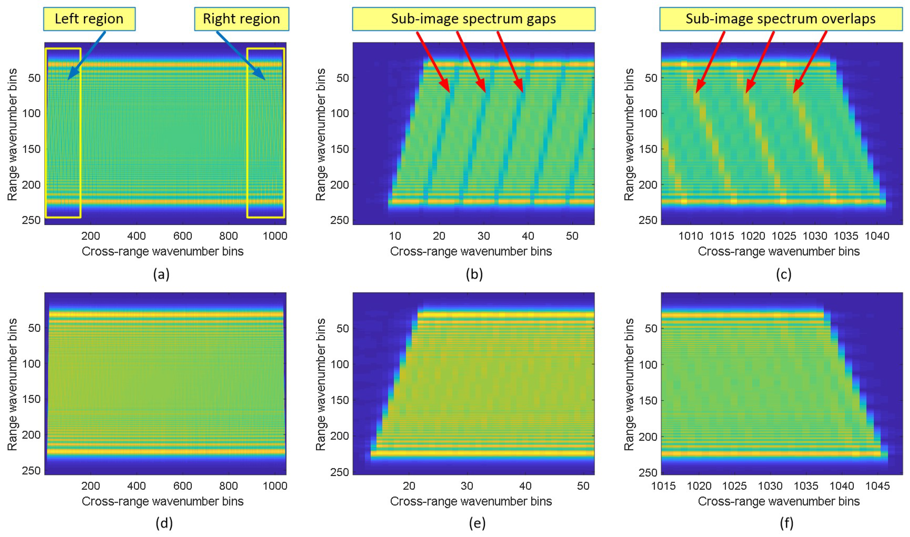
Figure 5.
Imaging result for linear trajectory. (a–c) are the target image, range profile and cross-range profile of AFBP, respectively. (d–f) are the target image, range profile and cross-range profile of HS-AFBP, respectively.
Figure 5.
Imaging result for linear trajectory. (a–c) are the target image, range profile and cross-range profile of AFBP, respectively. (d–f) are the target image, range profile and cross-range profile of HS-AFBP, respectively.

Figure 6.
3-D deviations in the nonlinear trajectory.
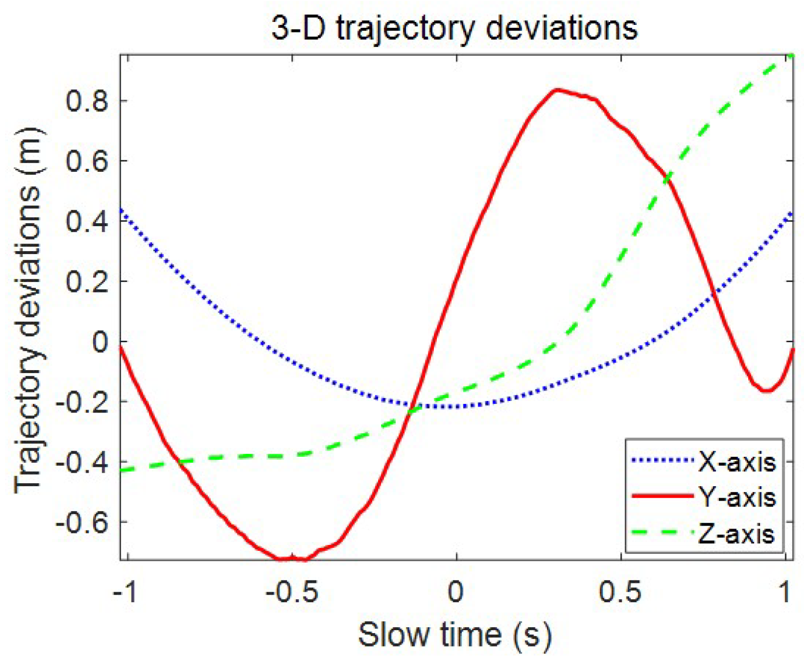
Figure 7.
Wavenumber spectrum of the 26th sub-image for nonlinear trajectory. For clarity, 2-D spectrum is presented here. (a) Original spectrum. (b) Spectrum after center correction using Equation (17). (c) Spectrum after center correction using Equation (23).

Figure 8.
Spectrum fusion for nonlinear trajectory. For clarity, 2-D spectrum is presented. (a) Whole aperture spectrum after fusion using Equation (17). (b,c) are the amplified sub-spectrum of the middle and right region in (a), respectively. (d) Whole aperture spectrum after fusion using Equation (23). (e,f) are the amplified sub-spectrum of the middle and right region in (d), respectively.

Figure 9.
Imaging result for nonlinear trajectory. (a–c) are the target image, range profile and cross-range profile focused by Equation (17), respectively. (d–f) are the target image, range profile and cross-range profile focused by Equation (23), respectively.

Figure 10.
Flowchart of the proposed HS-AFBP algorithm.
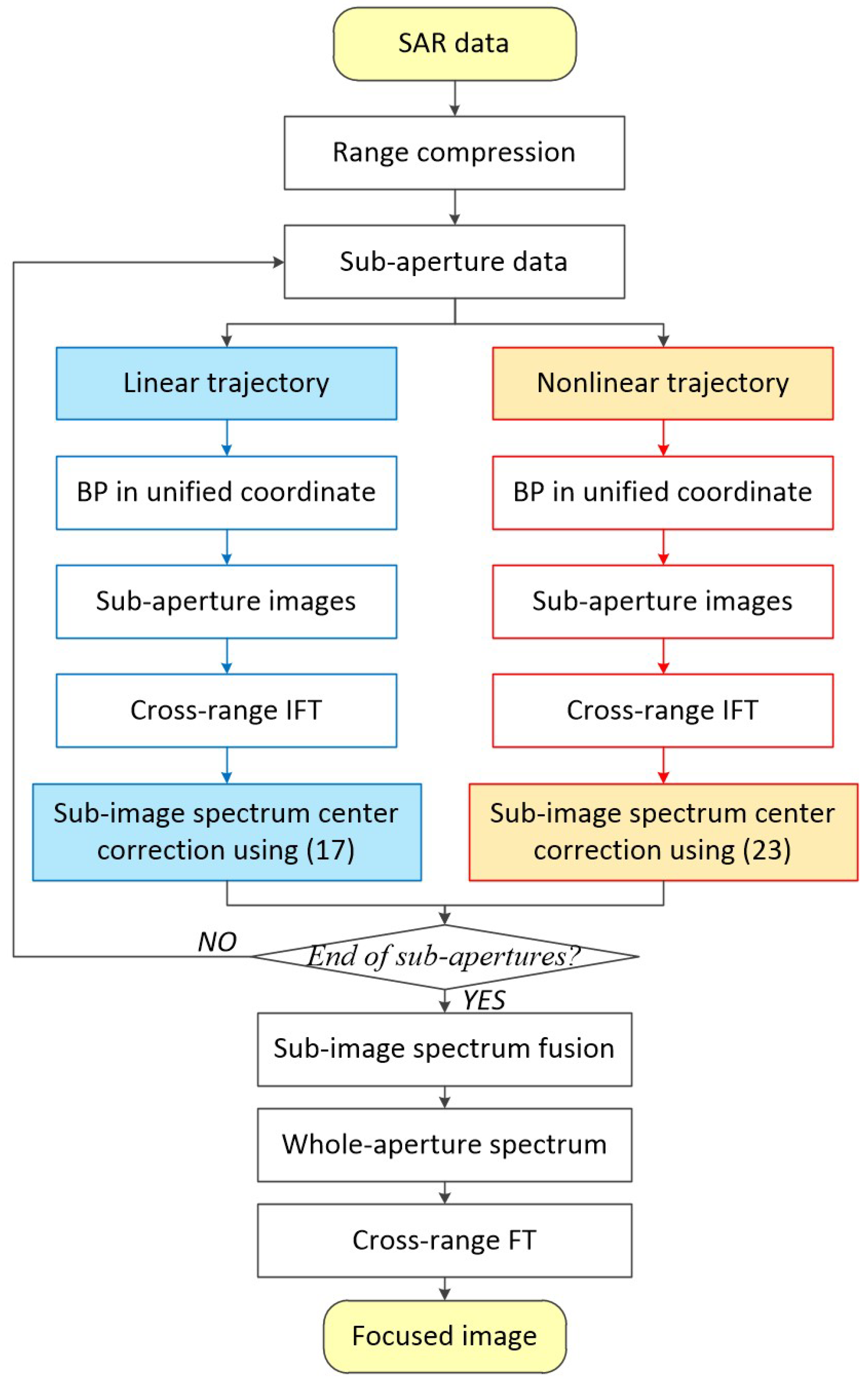
Figure 11.
Trajectory deviations in dataset 1.

Figure 12.
The first sub-image spectrum in dataset 1. For clarity, 2-D spectrum is presented. (a) Original spectrum. (b) Spectrum corrected by AFBP. (c) Spectrum corrected by HS-AFBP.
Figure 12.
The first sub-image spectrum in dataset 1. For clarity, 2-D spectrum is presented. (a) Original spectrum. (b) Spectrum corrected by AFBP. (c) Spectrum corrected by HS-AFBP.

Figure 13.
Final imaging results in dataset 1. (a) Image of AFBP. (b) Image of HS-AFBP.

Figure 14.
Local images in dataset 1. In each pair of local images, the left one is obtained by AFBP, and the right one is the result of HS-AFBP. The image entropy is presented at the title of each local image. HS-AFBP always achieves smaller entropy values, which outperforms the conventional AFBP in terms of focusing ability.

Figure 15.
Target cross-range profiles comparison in dataset 1. (a) Target T1 as circled in Figure 14b. (b) Target T2 as circled in Figure 14c.

Figure 16.
Trajectory deviations of dataset 2.
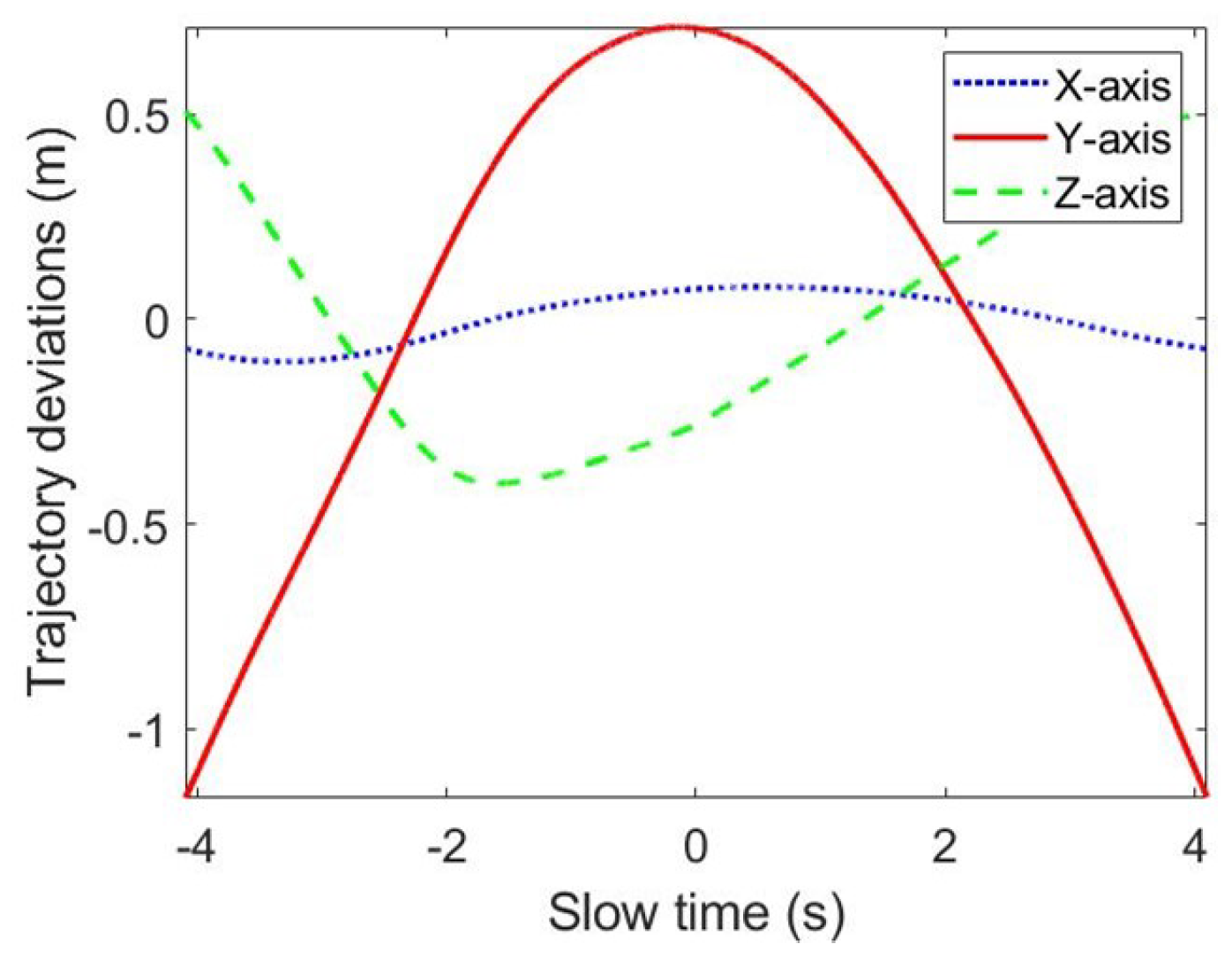
Figure 17.
The spectrum of the 53rd sub-image in dataset 2. For clarity, 2-D spectrum is presented. (a) Original spectrum. (b) Spectrum corrected by AFBP. (c) Spectrum corrected by HS-AFBP.
Figure 17.
The spectrum of the 53rd sub-image in dataset 2. For clarity, 2-D spectrum is presented. (a) Original spectrum. (b) Spectrum corrected by AFBP. (c) Spectrum corrected by HS-AFBP.
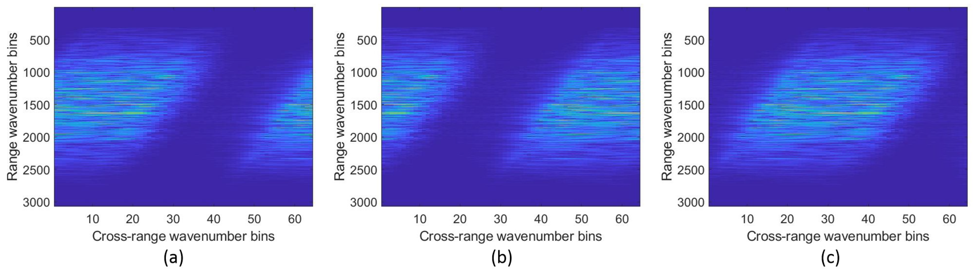
Figure 18.
Spectrum fusion in dataset 2. For clarity, 2-D spectrum is presented. (a) Whole aperture spectrum fused by AFBP. (b,c) are the left and right regions in (a), respectively. (d) Whole aperture spectrum fused by HS-AFBP. (e,f) are the left and right regions in (d), respectively. The sub-image spectrum gaps and overlaps are very obvious in AFBP processing, while the HS-AFBP fused spectrum is smooth and continuous.
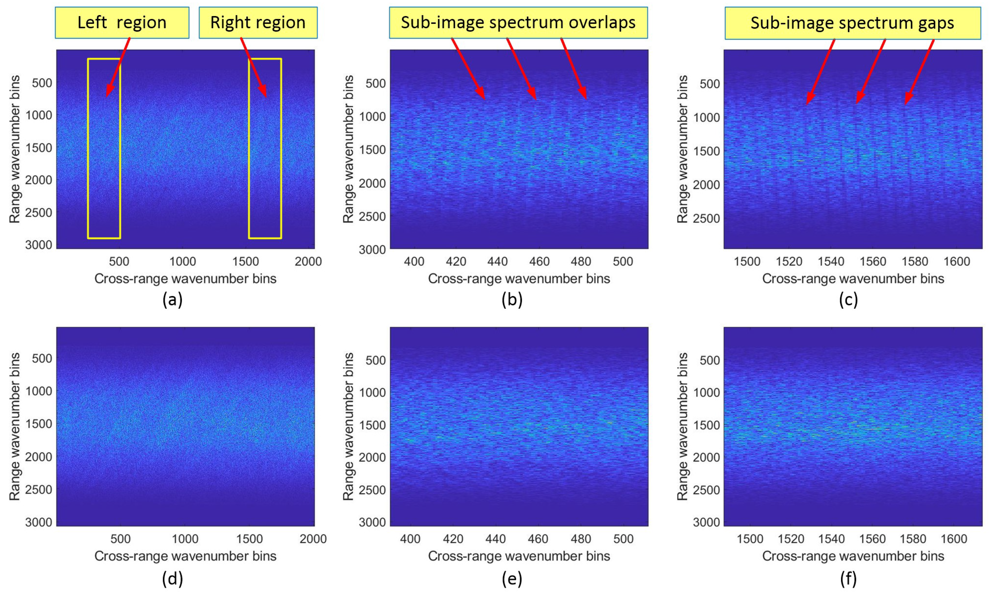
Figure 19.
Final imaging results in dataset 2. (a) Image of AFBP. (b) Image of HS-AFBP.

Figure 20.
Local images in dataset 2. In each image pair, the left one is obtained by AFBP, and the right one is the result of HS-AFBP. The image entropy is presented at the title of each local image. HS-AFBP exhibits clearer ground details and smaller entropy values than AFBP results.
Figure 20.
Local images in dataset 2. In each image pair, the left one is obtained by AFBP, and the right one is the result of HS-AFBP. The image entropy is presented at the title of each local image. HS-AFBP exhibits clearer ground details and smaller entropy values than AFBP results.

Figure 21.
Target cross-range profiles comparison in dataset 2.


Table 1.
Simulated SAR parameters for linear trajectory.
| Parameter | Value |
|---|---|
| Operational band | |
| Operational range | 10 km |
| Bandwidth | 300 MHz |
| Squint angle | |
| Whole aperture length | m |
| Sub-aperture length | m |
| Scene center (range, azimuth) | m |
| Target position (range, azimuth) | m |
Table 2.
Radar and geometry parameters in real data experiments.
| Parameter | Dataset 1 | Dataset 2 |
|---|---|---|
| Operational band | ||
| Bandwidth | 200 MHz | 200 MHz |
| Squint angle | ||
| Operational range | km | km |
| Altitude | km | km |
| Synthetic aperture length | m | m |
| Scene size (range × cross-range) | 1.23 km × 1.09 km | 1.85 km × 0.92 km |
Table 3.
Focusing quality comparison in dataset 1.
| Methods | T1 | T2 | ||||
|---|---|---|---|---|---|---|
| PSLR (dB) | ISLR (dB) | Resolution (m) | PSLR (dB) | ISLR (dB) | Resolution (m) | |
| AFBP | −1.69 | −4.34 | 2.24 | −4.72 | −7.36 | 2.09 |
| HS-AFBP | −19.40 | −14.37 | 0.72 | −13.71 | −12.88 | 0.69 |
Table 4.
Focusing quality comparison in dataset 2.
| Methods | PSLR (dB) | ISLR (dB) | Resolution (m) |
|---|---|---|---|
| AFBP | −11.70 | −11.58 | 0.96 |
| HS-AFBP | −13.73 | −12.21 | 0.89 |
© 2019 by the authors. Licensee MDPI, Basel, Switzerland. This article is an open access article distributed under the terms and conditions of the Creative Commons Attribution (CC BY) license (http://creativecommons.org/licenses/by/4.0/).
Share and Cite
MDPI and ACS Style
Ran, L.; Liu, Z.; Xie, R.; Zhang, L. Focusing High-Squint Synthetic Aperture Radar Data Based on Factorized Back-Projection and Precise Spectrum Fusion. Remote Sens. 2019, 11, 2885. https://doi.org/10.3390/rs11242885
AMA Style
Ran L, Liu Z, Xie R, Zhang L. Focusing High-Squint Synthetic Aperture Radar Data Based on Factorized Back-Projection and Precise Spectrum Fusion. Remote Sensing. 2019; 11(24):2885. https://doi.org/10.3390/rs11242885
Chicago/Turabian StyleRan, Lei, Zheng Liu, Rong Xie, and Lei Zhang. 2019. "Focusing High-Squint Synthetic Aperture Radar Data Based on Factorized Back-Projection and Precise Spectrum Fusion" Remote Sensing 11, no. 24: 2885. https://doi.org/10.3390/rs11242885
Note that from the first issue of 2016, this journal uses article numbers instead of page numbers. See further details here.