Analysis of Stochastic Distances and Wishart Mixture Models Applied on PolSAR Images
by
Naiallen Carolyne Rodrigues Lima Carvalho
*,†, 
Leonardo Sant’Anna Bins
† and
Sidnei João Siqueira Sant’Anna
† Image Processing Division, National Institute for Space Research (INPE/DPI), Astronautas Av., 515, São José dos Campos, São Paulo 12227-010, Brazil
*
Author to whom correspondence should be addressed.
†
These authors contributed equally to this work.
Remote Sens. 2019, 11(24), 2994; https://doi.org/10.3390/rs11242994
Submission received: 31 October 2019
/
Revised: 28 November 2019
/
Accepted: 9 December 2019
/
Published: 12 December 2019
(This article belongs to the Special Issue Selected Papers from the Polarimetric Interferometric SAR Workshop 2019)
Abstract
:This paper address unsupervised classification strategies applied to Polarimetric Synthetic Aperture Radar (PolSAR) images. We analyze the performance of complex Wishart distribution, which is a widely used model for multi-look PolSAR images, and the robustness of five stochastic distances (Bhattacharyya, Kullback-Leibler, Rényi, Hellinger and Chi-square) between Wishart distributions. Two unsupervised classification strategies were chosen: the Stochastic Clustering (SC) algorithm, which is based on the K-means algorithm but uses stochastic distance as the similarity metric, and the Expectation-Maximization (EM) algorithm for Wishart Mixture Model. With the aim of assessing the performance of all algorithms presented here, we performed a Monte Carlo simulation over a set of simulated PolSAR images. A second experiment was conducted using the study area of Tapajós National Forest and the surrounding area, in Brazilian Amazon Forest. The PolSAR images were obtained by the satellite PALSAR. The results, in both experiments, suggest that the EM algorithm and the SC with Hellinger and the SC with Bhattacharyya distance provide a better classification performance. We also analyze the initialization problem for SC and EM algorithms, and we demonstrate how the initial centroid choice influences the final classification result.
1. Introduction
Synthetic Aperture Radar (SAR) image classification has an important role in socioeconomic applications, and it has become fundamental in environmental monitoring. The major advantages of SAR sensors are daylight independence, less influence of weather, and, depending on the wavelength, clouds, dust, or even the vegetation canopy would be transparent to the sensor’s frequency spectrum. In addition, the use of PolSAR (Polarimetric Synthetic Aperture Radar) images, which measures the target backscattering in different polarization, can provide further information such as soil moisture, surface roughness, target shape, and geometry.
Although PolSAR system can provide high spatial resolution images, those are contaminated by an interference pattern called speckle, a common phenomenon on coherent systems, which cannot be avoided. The speckle causes a granular pattern in SAR images, making the analysis of objects contained within the image difficult, and it can lead to a reduction in classification accuracy and segmentation effectiveness [1]. Nevertheless, the speckle has rich statistical information, which can be explored by attributes derived from Information Theory, such as divergences [2], entropy [3] and, as explored in this work, stochastic distances [4]. Stochastic distances are any non-negative, symmetric function between two Probability Density Functions (PDF), which obeys the triangular inequality [5].
Understanding PolSAR speckle statistic is essential to have a good comprehension about the scattering mechanisms. Hence, a huge effort to characterize the statistical properties of PolSAR images has been done, for instance, by [5,6,7,8]. The statistical analysis can improve the PolSAR image interpretation by presenting the proper statistical distribution to model it, helping to develop smart algorithms for speckle filtering [9], segmentation [10,11,12], feature extraction [13] and classification [14,15,16,17].
Classification is one of the most important tools for image interpretation and analysis. It consists of assigning the same label to a set of data samples that share common properties, with the goal of reducing the amount of information and simplify the data interpretation. Classification methods can be either supervised or unsupervised. Supervised classification requires prior information (training samples), while in unsupervised classification the prior information is not available, therefore a common way of performing unsupervised classification relies on clustering algorithms.
The main goal of clustering techniques is to maximize the inner cluster homogeneity and the inter clusters heterogeneity based on the data set natural evidence of division. However, to cluster a data set, from which no information is known, could be a difficult task, even harder in noise and interference presence. Therefore, seeking for an appropriated clustering technique is imperative to reach an optimum classification result. The fundamental challenges on clustering technique choosing are the identification of:
- (a)
- Data set type (numerical real, numerical complex, categorical);
- (b)
- Data set normalization need;
- (c)
- Outliers, and how to deal with them;
- (d)
- Number of clusters;
- (e)
- Cluster shape;
- (f)
- Similarity measure;
- (g)
- The initial centroid location choice.
The proper statistical model definition helps to characterize the data set and to derive information about outliers, cluster shape, and the appropriated similarity measure. For instance, assuming a data set following a multivariate Gaussian distribution (multi-look PolSAR image in amplitude, for example), its covariance matrix defines the cluster shape. Considering the hyperspherical shaped cluster, the Euclidean distance would be suitable in this case. On the other hand, if the cluster has an elongated shape, a better approach would be to apply the Mahalanobis distance. Notwithstanding PolSAR images could be represented by its second-order polarimetric representation, this covariance matrix carries information about the target geometry rather than data set spreading behavior, as in the Gaussian PDF model. Therefore, new clustering techniques must be devised in order to handle PolSAR data properly.
In this work, we present a study about PolSAR image classification using two well-established clustering algorithms: the EM (Expectation-Maximization) and K-means. The EM algorithm softly assigns a sample to clusters, i.e., the EM computes the sample probability of being assigned to a cluster. Commonly, the EM algorithm estimates the parameters of a Gaussian mixture model. However, PolSAR images are widely known for following the Wishart distribution, for this reason, the EM presented here maximizes the Wishart mixture model distribution expectation. The K-means algorithm partitions the data set by minimizing the square root error between a sample and centroids, due to that, this algorithm is biased towards hyperspherical clusters, consequently, it fails when clusters tend to spread among different shapes. For this reason, we propose the use of stochastic distances as a similarity measure of the K-means algorithm, named, hereafter, Stochastic Clustering (SC) algorithm. In this work, we consider the following stochastic distances between Wishart Distribution: Bhattacharyya, Kullback-Leibler, Hellinger, Rényi of order and Chi-square.
This study aims to explore procedures for improving PolSAR image classification. We analyze seven classification algorithms—EM for Wishart mixture model distribution, SC using Bhattacharyya distance, SC using Kullback-Leibler distance, SC using Hellinger distance, SC using Rényi of order distance, SC using Chi-square distance, and the traditional K-means—applied in two experiments. The first experiment performs a Monte Carlo simulation over a set of simulated PolSAR images to find all possible classification outcomes for each algorithm, allowing us to produce a quantitative analysis of the results. In the second experiment, we applied the algorithms on an ALOS/PALSAR image from a Brazilian Amazon region.
This paper is organized as follows. Section 2 describes the PolSAR image representation and its multivariate complex Wishart distribution. In Section 3 the stochastic distances used in this work are presented. Section 4 presents how stochastic distances are applied to the K-means algorithm strategy. Section 5 defines the Wishart mixture model and describes how to estimate its parameters using the Expectation-Maximization algorithm. Section 6 shows the results of simulated images and a PolSAR image obtained by the satellite PALSAR. Section 7 presents the results discussion. Finally, our conclusions are presented in Section 8.
2. PolSAR Image Representation
The electromagnetic wave propagation is mainly characterized by its electrical field behavior, usually by its polarization. The polarization happens when the electrical field distorts the electrons cloud in a particular direction, being the linear a common polarization state. A SAR system that incorporates the linear polarization combinations between Vertical (v) and Horizontal (h) directions for transmitted and received waves is named PolSAR, and its images, when in QUAD-POL mode, could be represented by the scattering matrix , given by:
where , with x∈ representing the transmitted wave and y ∈ , representing the received wave, contains amplitude and phase information of a specific target. The elements on main diagonal are named ‘co-pol’ and the elements on secondary diagonal are named ‘cross-pol’.
The scattering behavior of targets in matrix depends, among other things, on the coordinate systems. The coordinate system considered in this work is the Back Scattering Alignment (BSA), where the transmitting and receiving antennas are collocated in space. Due to this, electromagnetic waves have a reciprocal medium. In the BSA coordinate system, the reciprocity theorem says that the cross-pol channels of the scattering matrix are equal, i.e., . Usually, for the studying of PolSAR statistical behavior, is more convenient to represent the matrix as a lexicographic basis vector [18]. Therefore, under the reciprocity theorem, the scattering vector could be expressed as:
The vector represents a single-look PolSAR data. Since PolSAR data is affected by speckle, a common approach to reduce the speckle is to perform the multi-look processing. From the statistical point of view, the multi-look processing is defined as the averaging of L neighboring samples, resulting in the covariance matrix defined in Equation (3).
where denotes the conjugate transpose, represents the complex conjugate and means the absolute value of a given number.
Let be a random variable data set with N samples and L number of looks. The matrix follows the complex multivariate Wishart distribution (Equation (4)). Therefore the PolSAR data can be described by the two Wishart parameters: the covariance matrix, where is related to image brightness and the number of looks L which is related to signal to noise ratio.
where , is the expectation operator, is the Gamma function, q is the covariance matrix order, is the matrix trace, and is the matrix determinant.
3. Stochastic Distances
Stochastic distance has its roots in information theory, which main concepts are entropy and information. The primary goal of entropy is to quantify the amount of information in a data set. Even though the entropy can provide the average rate of information produced from a stochastic process, it cannot measure whether a given PDF is more suitable to data set than another.
In order to overcome this task, Kullback and Leibler [19] introduced the relative entropy concept, also known as Kullback–Leibler divergence. This divergence computes the logarithmic difference between two distributions’ expectations. More generally, a divergence is any non-negative function that gauges the contrast between two PDF [5]. Following Kullback and Leibler [19] work, a number of divergence classes were developed, among then, Salicrú [20] defined the class of entropy , where h is a strictly increasing function and is a convex function.
Let and be random variables following Wishart distribution and having density and respectively, with parameter and , the divergence between and is given by [5]:
where A is sample space of positive defined matrices.
Changing the parameters h and , several divergences can be derived from Equation (5), for instance, the Bhattacharyya, Kullback-Leibler, Hellinger, Rényi of order and Chi-square. However, as the symmetry property is not necessarily satisfied, divergences cannot be defined as a metric. To address the symmetry problem, the simplest solution to generate a symmetric divergence is defined as [21]:
The function is defined as a distance, once the following properties are satisfied: non-negativity, symmetry, and definiteness. According with [5], distances between random variables which follows the same PDF, could be indexed by their parameters. Therefore, stochastic distances can be simplified into a distance between parameters . Assuming an equal number of looks L for the entire analysed data set, the distance could be summarized as a distance between covariance matrices . Based on that, Nascimento [8] derived the distances presented hereafter:
- Bhattacharyya
- Kullback-Leibler
- Hellinger
- Rényi of order
- Chi-square
where q is the matrix order, represents the matrix determinant, means the matrix trace, indicates the inverse of a matrix and abs(·) denotes the absolute value.
4. Stochastic Clustering Algorithm
Let be the data set of unknown samples to be clustered and be the set of K centroids, the K-means algorithm divides the data set x into K clusters based on the minimal Euclidean distance between a sample and a centroid . The association equation is represented as:
where if belongs to cluster , or otherwise, and represents the distance metric.
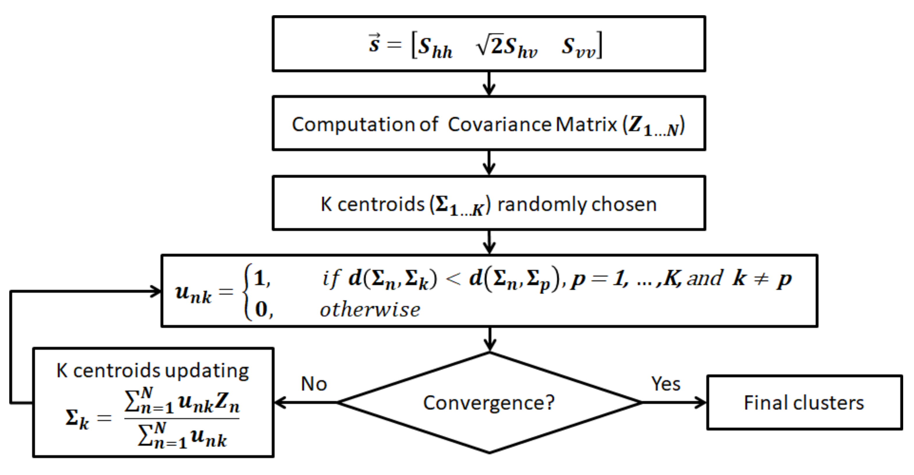
Typically the K-means algorithm handles data set in Euclidean Space, i.e., the data set x is represented as a m-tuple of real numbers defined by its centroid. However, the PolSAR covariance matrices set do not form an Euclidean space [22], therefore the Euclidean distance isn’t the most suitable metric to this kind of data. Indeed, in this work, we propose the use of stochastic distances, described in Section 3, as a similarity metric for K-means strategy, named Stochastic Clustering (SC). In this approach, the association equation is represented as:
and the rule for updating the cluster centroid is given by:
Figure 1 presents the steps of the SC algorithm. The first step consists in converting the PolSAR data into a set of covariance matrices , then the initial centroids are randomly selected. Thereupon, new partitions are generated by assigning each sample to its closest cluster center by applying Equation (13). The algorithm convergence is verified. If this verification fails, the centroids are updated using Equation (14), otherwise, the final clustering is achieved.
The time complexity of K-means algorithm, and, therefore, the time complexity of the Stochastic Clustering algorithm, depends upon inputs parameters definition. If the number of centroids are fixed, then the problem admits polynomial-time approximation schemes. Moreover, when the number of centroids (K), number of samples (N) and number of iterations (i) are defined, the K-means has complexity [23]. In this work we defined and , therefore the complexity is .
5. Expectation Maximization of Wishart Mixture Model
The EM algorithm is an iterative procedure that uses the maximum a posteriori rule to compute the maximum likelihood of a mixture model distribution. Assuming as set of observed complex covariance matrices, the Wishart mixture model can be expressed by [24]:
where K is the number of Wisharts within the mixture, is the mixture model parameter vector and is the weighting factor per Wishart. Since the EM must be executed over all samples, the complete-data log likelihood is formulated as:
where if the sample n produces a measurement k, and otherwise.
At every iteration the EM algorithm consists in two steps:
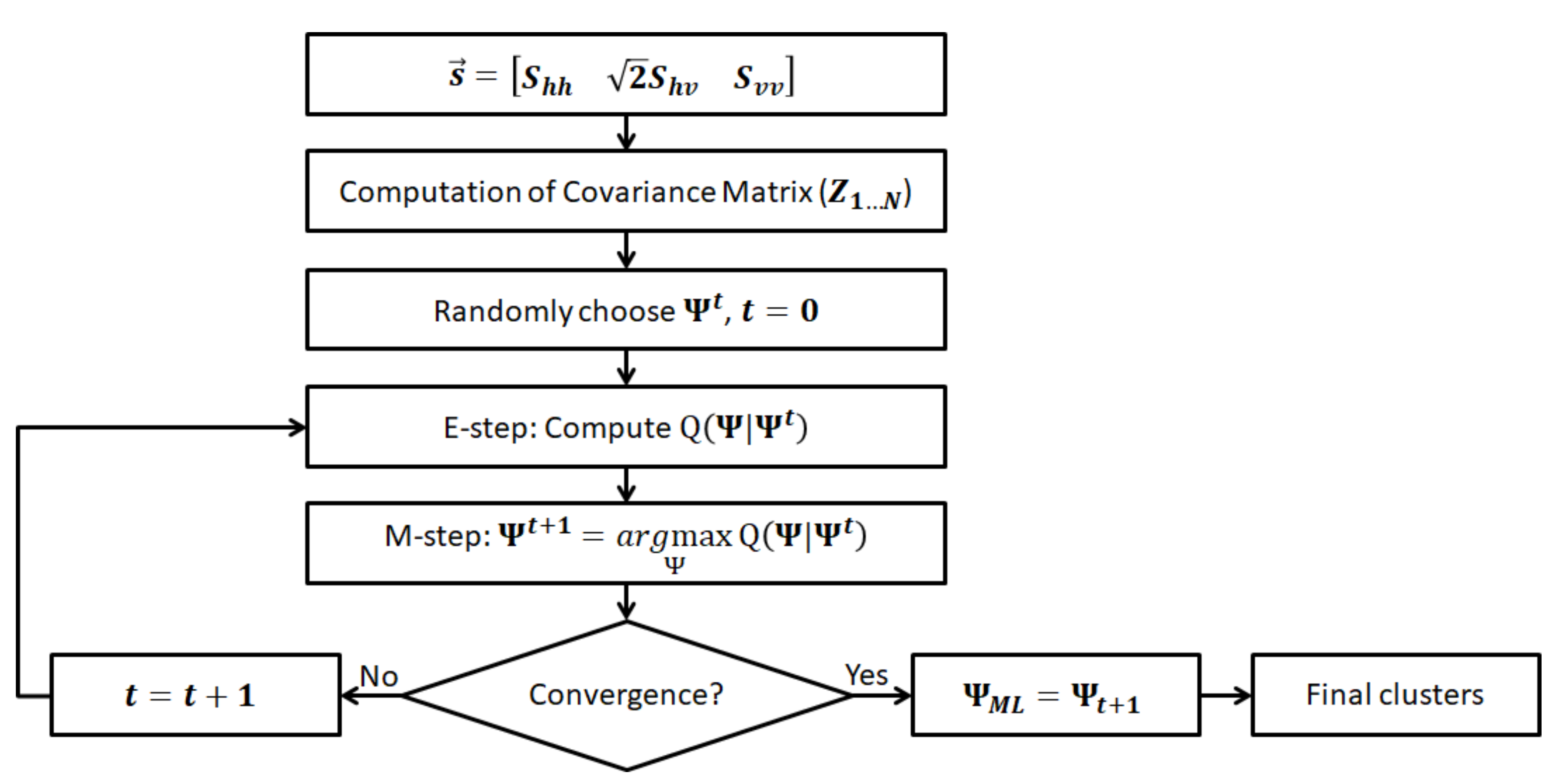
- The Expectation or E-step. In E-step the log-likelihood of the observed data , given the estimated parameter , is calculated as:
- The Maximization or M-step. The M-step finds the new estimation by maximizing :Since the parameter is composed of and , the parameter optimization is done by setting the respective partial derivative to zero. The optimization with respect to can be summarized as:and the new estimation for is given by:
Figure 2 shows the steps applied for the EM algorithm. In the beginning, the PolSAR data sample shall be upload and transformed into covariance matrices. After that, the EM steps are executed: first the E-step followed by the M-step; the convergence is checked and if the algorithm does not converge, then the parameters are updated, otherwise, the final clustering is computed.
The EM algorithm, as SC algorithm, has time complexity , where K is the number of centroids, N is the number of samples and i number of iterations. In the same way as for SC algorithm, and , therefore the complexity is .
6. Applications
In this study we address the unsupervised PolSAR image classification topic and explore the potential of stochastic distances applied to clustering techniques by classifying PolSAR images with the following techniques:
- Expectation-Maximization for Wishart mixture model distribution (EM-W);
- Stochastic Clustering using Bhattacharyya distance (SC-B);
- Stochastic Clustering using Kullback-Leibler distance (SC-KL);
- Stochastic Clustering using Hellinger distance (SC-H);
- Stochastic Clustering using Rényi of order distance (SC-R). The selected value of the Rényi’s order () was 0.9;
- Stochastic Clustering using Chi-square distance (SC-C).
- K-means using Euclidean distance (KM-E);
In order to quantify the sensitiveness of the techniques above-mentioned a Monte Carlo simulation over a set of one hundred simulated PolSAR images was conducted, the experiment description can be found in Section 6.1. Aiming to ratify the Monte Carlo simulation results a second experiment was conducted using an ALOS/PALSAR image from a Brazilian Amazon forest region, the experiment description and classification results are discussed in Section 6.2.
6.1. Experiment I
6.1.1. Image Simulation
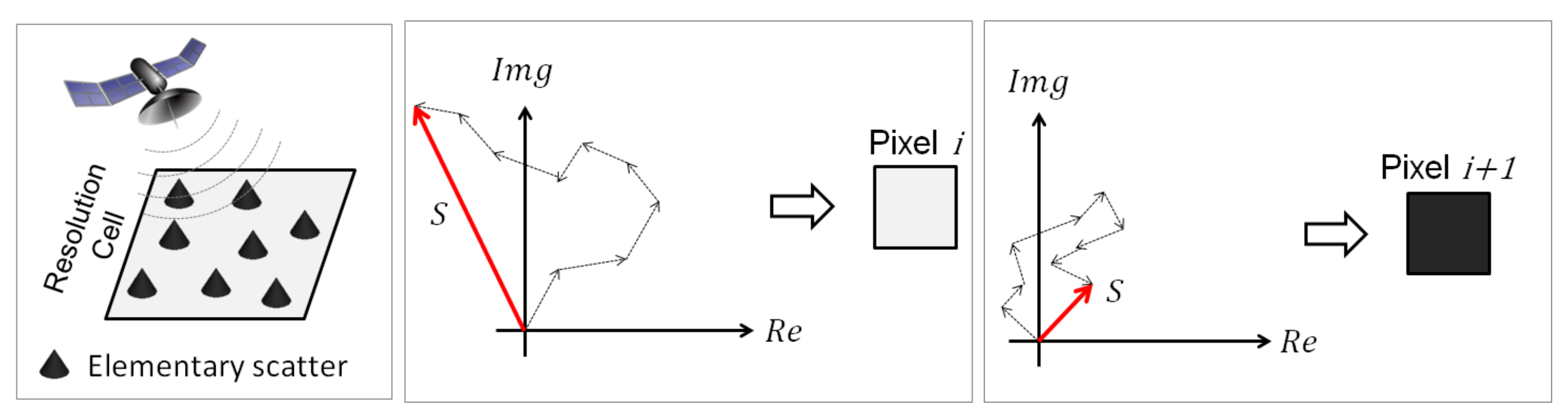
Electromagnetic signals emitted by the radar interacts with elementary scatterers within a resolution cell, as shown in Figure 3a. The elementary scatterers reflect the signal and part of the backscattering is detected by the radar receiver antenna. The received signal S, which will be later transformed into an image pixel value, is the result of a coherent sum of W waves reflected by many elementary scatterers, and it is defined by Equation (21):
where .
If the scatters returns are constructively added, the signal will be stronger, as shown in Figure 3b. However, if the returned waves are out of phase, then the signal will be destructively added, resulting in a weak signal, as shown in Figure 3c. Due to that, a pixel-to-pixel variation in intensities appears on radar images.
In this work, for simulation purposes, only smooth surface scenarios are considered. The surface roughness is defined by the Rayleigh Criterion, which says that a surface is smooth if , where is the standard deviation of surface roughness, is the radar wavelength and is the incident angle. Given a smooth surface, where there is no dominant scatterer and where the number of scatterers is large, by the Central Limit theory, the components and are assumed to be identically Gaussian distributed with zero mean and a variance denoted as [1].
Since the PolSAR scattering information can be represented by a complex vector , follows a circularly symmetric multivariate complex Gaussian distribution, denoted by . Under the assumption of circular symmetry of , the pixel simulation is done by sampling the vector with real values , such that [25], where is described as:
where and represents the real and imaginary part of a complex number.
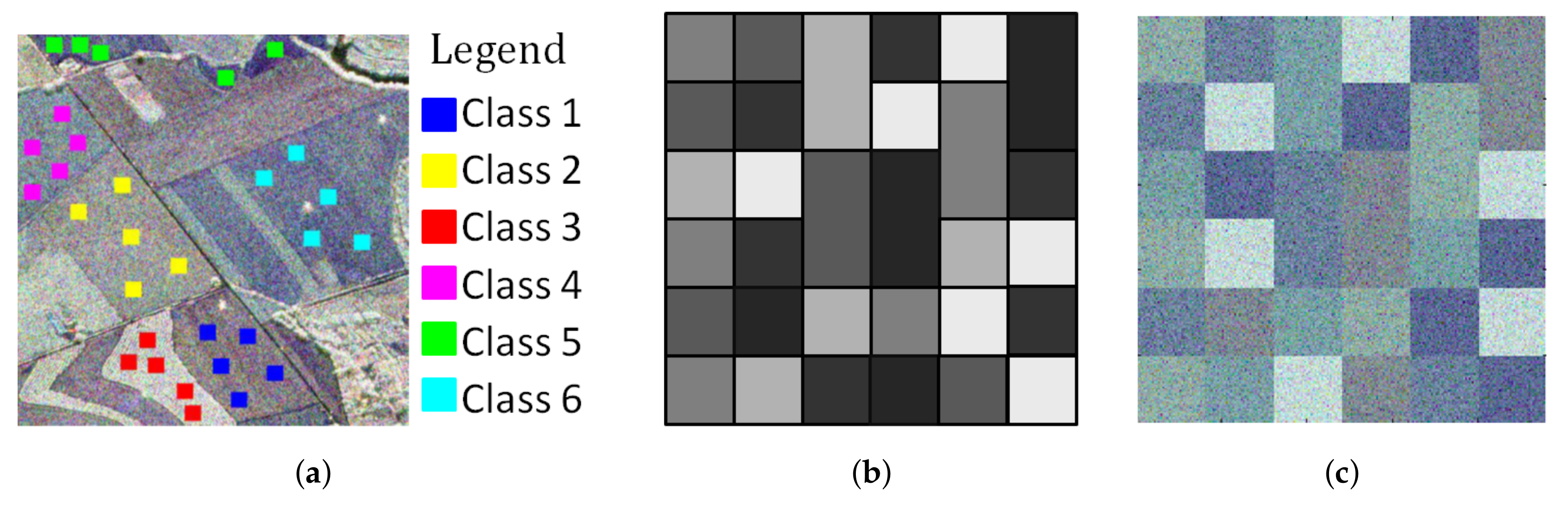
The covariance matrices , used in the simulation process, were estimated from a PolSAR image acquired by the airborne sensor SAR-R99B in L-band from the Brazilian SIVAM (Amazon Surveillance System). The 1-look image, presented in Figure 4a, has polarization . Table 1 presents the average complex covariance matrices, estimated from five samples taken from the 1-look image (Figure 4a). Since the covariance matrix is Hermitian, only the upper triangle is presented in Table 1.
According to [5] the number of looks alters the data set distribution in a non-linear way, which can be perceived by the stochastic distances. As lower the number of looks, more sensitive are the distances to smaller differences between classes, leading to a noisier classification result. In this work, we choose to simulated the images with a low number of looks in order to identify the distances with robustness to noise.
The simulated images, with 3 looks, were obtained from a phantom image (Figure 4b) sizing 240 by 240 pixels. The phantom image contains 36 segments sizing 40 by 40 pixel each. One example of a simulated image is shown in Figure 4c, this image is a color composition of PolSAR in amplitude, where , and .
6.1.2. Monte Carlo Simulation Results
The SC, EM, and K-means are greedy algorithms [26], i.e., they are algorithms that make a locally optimal choice at each stage with the goal of finding the global optimal solution to the entire problem. Due to that, those algorithms usually converge to a local minimum, being able to converge to the global optimum when clusters are well separated. Therefore a Monte Carlo simulation is conducted in this work in order to perform the analysis of clustering convergence and the overall classification accuracy.
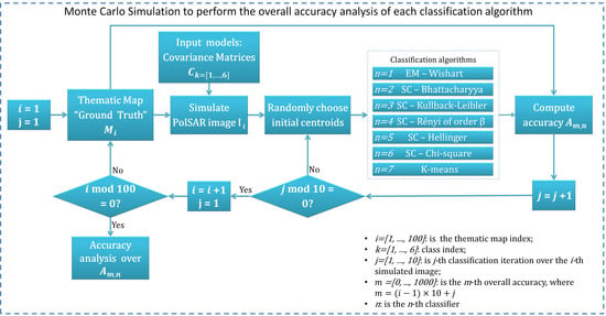
The Monte Carlo simulation allows the accuracy analysis of the seven above-cited algorithms: EM-W, SC-B, SC-KL, SC-H, SC-R, SC-C, and KM-E, in order to determine which algorithm gives the best classification. At each Monte Carlo iteration, the algorithms shared the same initial parameters: number of classes, initial centroids, and number of algorithm iteration. All computations were based on a set of one hundred randomly simulated PolSAR images, where each simulated image was tested ten times for different algorithm’s initial parameters. It means that one thousand Monte Carlo iterations were executed for each algorithm. In this experiment the simulated images contain six classes, the initial centroids are randomly chosen and the algorithms stop criteria is the number of iteration equal to five.
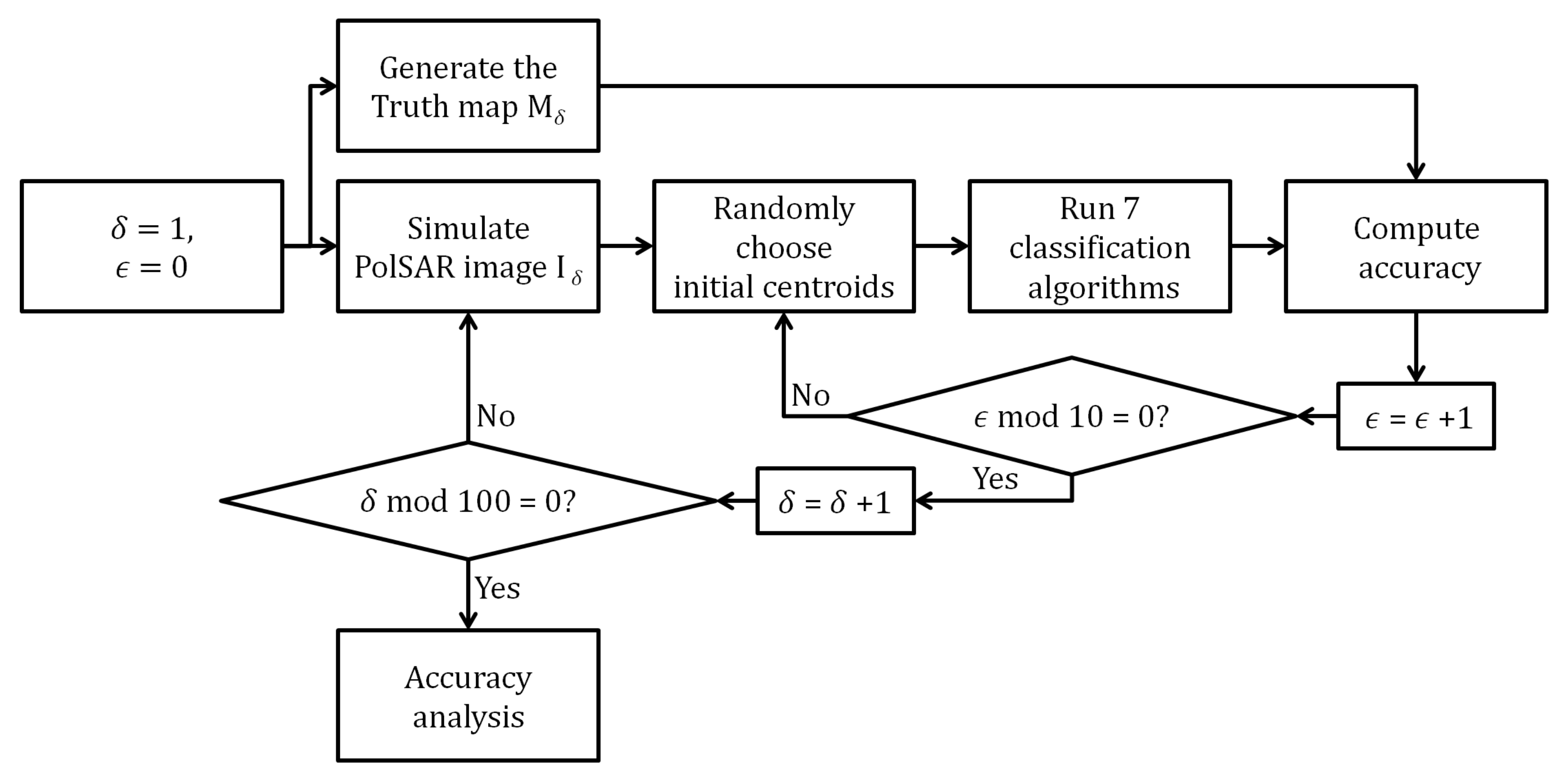
The flowchart of the Monte Carlo Simulation is outlined in Figure 5. The first step consists of simulating PolSAR image and generating its Truth Map, which will be later used as true values for computing the classification overall accuracy. Then, K initial centroids are randomly chosen. In the next step, the seven classifications are executed, and the overall accuracy of all classification is computed. Each image pass through the Monte Carlo Simulation steps ten times, and after one thousand iterations, the Monte Carlo Simulation stops.
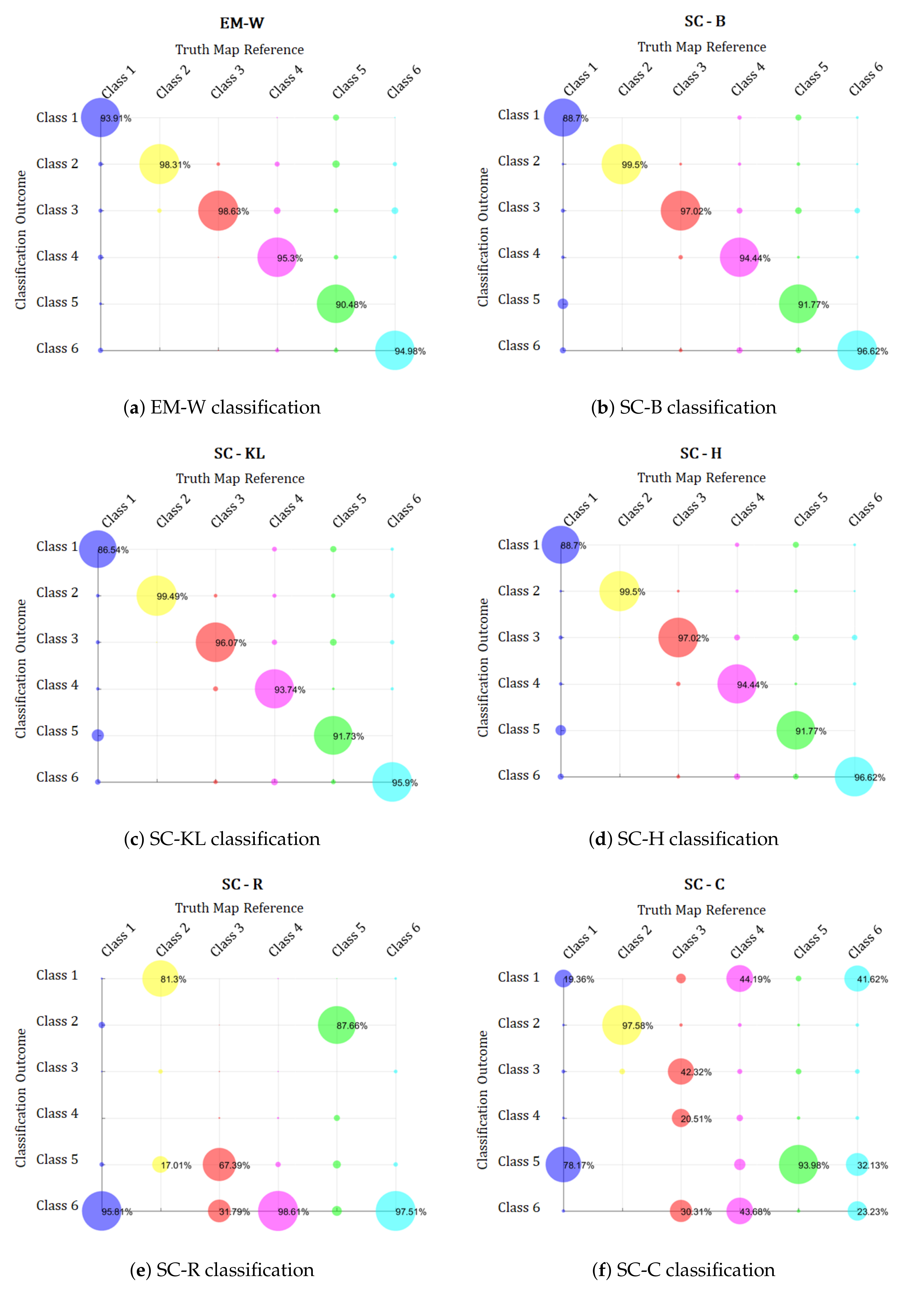
The overall accuracy values were obtained from a confusion matrix , where the true condition was given by the Truth map and the outcome condition was given by the classification result. The elements , with , of main diagonal, represent the number of samples corrected classified, i.e., the outcome label is equal to the true label; while off-diagonal elements , with , represents the misclassified samples. The overall accuracy is defined as:
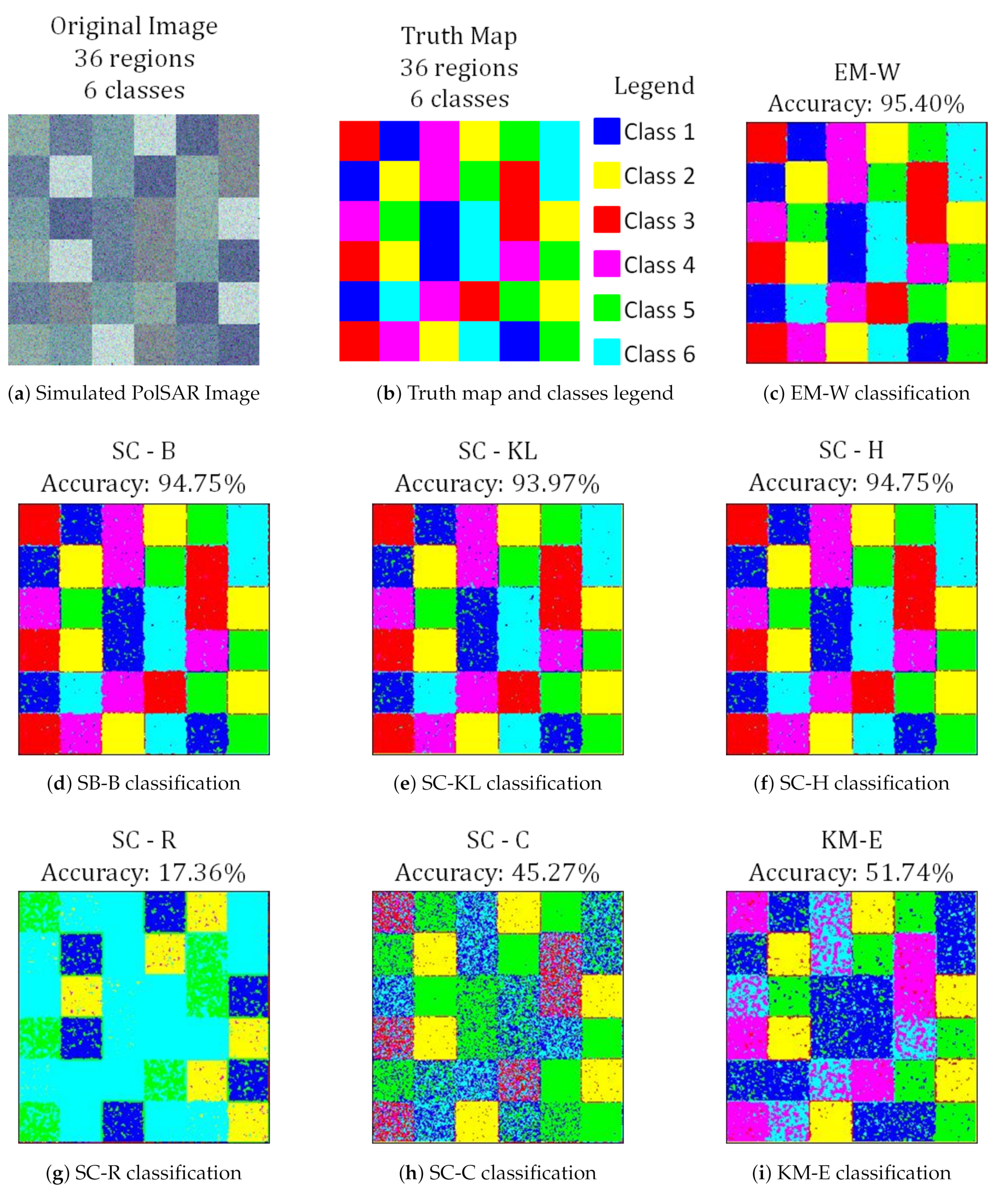
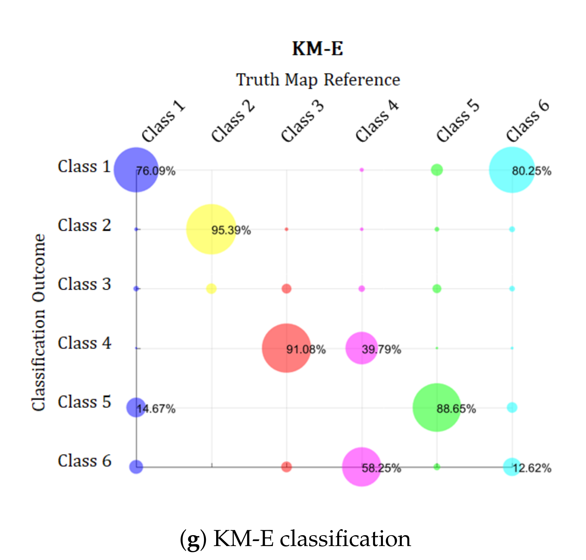
Figure 6 presents one simulated image example (Figure 6a) followed by its truth map (Figure 6b) and the classification result of algorithms: EM-W, SC-B, SC-KL, SC-H, SC-R, SC-C and KM-E, generated by one Monte Carlo simulation iteration. Figure 7 presents the respective confusion matrix of each result showed in Figure 6. The confusion matrix is presented in a bubble chart type of chart, where three dimensions are considered: the truth map in horizontal axis, the classification outcome in vertical axis and the third dimension is the confusion matrix elements value or size, which are represented in perceptual form, therefore the confusion matrix column shall be added up to . The values are displayed at the confusion matrix chart only if they are higher than .
The particular result presented in Figure 6 shows a better performance of statistical approaches over the traditional method KM-E, except for SC-R and SC-C. The EM-W had the best classification result, displayed in Figure 6c, achieving of overall accuracy, and the respective confusion matrix graph (Figure 7a) shows that this result had little confusion between classes, what directly reflects on its high accuracy result.
The SC-B classification (Figure 6d) also had a good result, achieving of overall accuracy. The Bhattacharyya distance is widely used to evaluate class separability, being an efficient tool for image segmentation and classification, and this efficiency is verified in the SC-B confusion matrix graphic (Figure 7b). In this graph, the values of the outcomes are concentrated in the main diagonal and the degree of uncertainty is low. The SC-H classification (Figure 6f) had an analogous result as SC-B, what is excepted due to the close relationship between the Hellinger and Bhattacharyya distance. The SC-KL classification (Figure 6e) achieved a quite similar result to SC-H and SC-B classification results, however, it had a slightly bigger degree of misclassification between Class 1 and Class 5, these two classes have similar intensity values (see Table 1).
The SC-R had the worst classification result, with only of overall accuracy. According to [8] the Rényi of order under the structure has a complicated analytic expression that can lead to numerical instabilities. Since the simulated image has low covariance matrices values (see Table 1) the numerical errors of Rényi of order could be high enough to prevent the algorithm discrimination between classes, as can be seen at SC-R confusion matrix graph (Figure 7e). This graph shows that the misclassification occurs, mainly, with Class 1, Class 4 and Class 6, while the classes with higher or lower covariance matrix values are well discriminated, even though wrongly labeled.
The SC-C also had a bad overall accuracy result () and this could be explained by the nature of this distance. The Chi-square distance is derived from Pearson’s chi-squared statistical test which is used for comparing discrete probability distributions, for instance, histograms. Therefore this distance struggles to discriminate small variances between classes [27], as can be seen in SC-C confusion matrix graph (Figure 7f), this algorithm has the noisier classification result. Finally, the KM-E classification also had a bad overall accuracy result () and was not able to correctly classify the pixels from Class 6, misclassifying those as Class 1. As SC-C, the KM-E also has a noisier classification result.
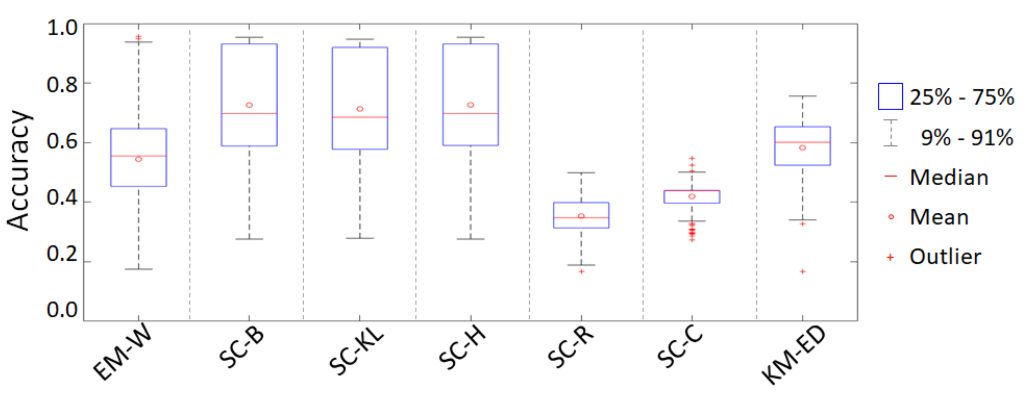
Figure 8 synthesizes the Monte Carlo simulation classification accuracy outputs. In this graph, on each blue box, the bottom and top edges indicate the 25th and 75th percentiles of the overall accuracy outcomes, the central red mark indicates the median accuracy, the red circle indicates the mean accuracy and the outliers are plotted individually using the ‘+’ symbol in red.
The overall accuracy of EM-W algorithm, provided by the Monte Carlo simulation and showed in Figure 8, presents the highest dispersion, meaning that some classifications are really good and others really bad, while the average accuracy is between and . Factors that influence the clustering performance are the algorithm convergence criteria or the number of iterations, initial centroid, outliers and so on. Since the number of iteration is fixed in five, the EM-W algorithm may not converge during this limited number of iteration leading to low accuracy results. The SC-B, SC-KL, SC-H have the most balanced results, were the first quartile and third quartile are between and . Those algorithms have the same number of iteration as the EM-W, therefore SC-B, SC-KL, SC-H may converge to the local optimum quicker than EM-W. As excepted the SC-R and SC-C presents the lower and less dispersed accuracy values. The KM-E has a medium result, having the first quartile and third quartile between and
According to results shown in Figure 8 and Table 2, higher mean accuracy values were obtained for SC-H, SC-B, SC-KL algorithms respectively, followed by the KM-E, EM-W, and the worst classification results came with SC-R and SC-C. However, the accuracy standard deviation, for all algorithms, are reasonable, especially for SC-H, SC-B and SC-KL algorithms, which indicates a high dependency of those algorithms on the choice of initial centroids.
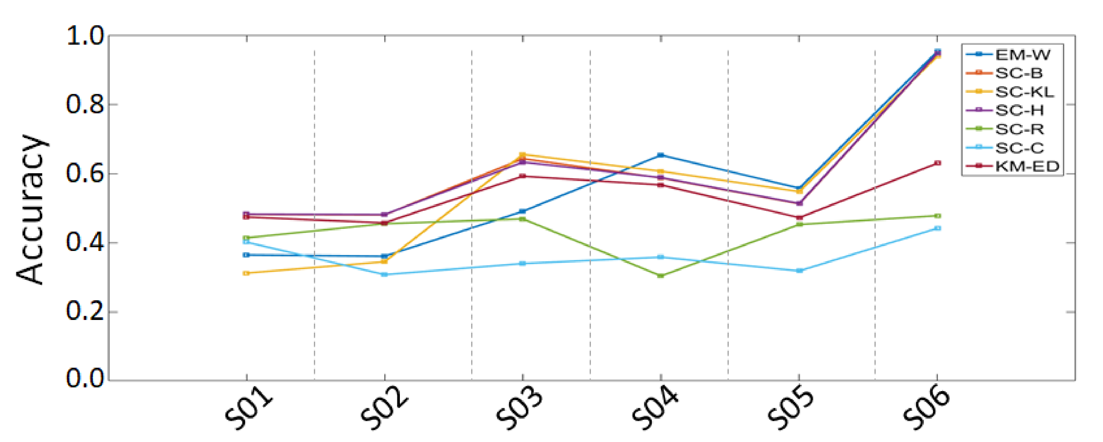
Frequently, the algorithms analyzed in this work can be trapped in a local minimum, which led to incorrect clustering results. One of the reasons why this happens is the choice of initial centroids. Bad initial centroids choosing happens when the centroids are selected from the same class, or when they are in the border of two classes, and especially it comes from the overlays. In order to investigate the initial centroids dependency, a simulated PolSAR image containing six classes was selected and the classifications were performed considering six different scenarios:
- S01: All six initial centroids were selected from the one class;
- S02: The six initial centroids are distributed over three class;
- S03: The six initial centroids were picked from the borders of two classes;
- S04: Three initial centroids were selected in three different class, and the other three comes from the borders of two classes;
- S05: All initial centroids comes from overlays;
- S06: One initial centroid were picked per class.
Figure 9 and Table 3 shows the accuracy results for each classification algorithm per scenario, by those results, it can be seen that, even when the initial centroid is not good, the SC-H, SC-B have a better classification accuracy overall algorithms. However when the centroids have a good fit, i.e., when the centroids are taken from scenario S06, the accuracy results achieves high accuracy for EM-W, SC-H, SC-B, and SC-KL algorithm, with 95.29%, 94.77%, 94.67%, and 93.91% of accuracy respectively, while KM-E, SC-R, and SC-C present just a slightly better accuracy results for scenario S06 in comparison with others scenarios.
Table 4 presents the execution time for each algorithm analysed in this work. All computations were performed in a computer with Intel Core i7 2.4GHz processor, 8GB of RAM, and Matlab 2018.
6.2. Experiment II
6.2.1. ALOS PALSAR Image Description
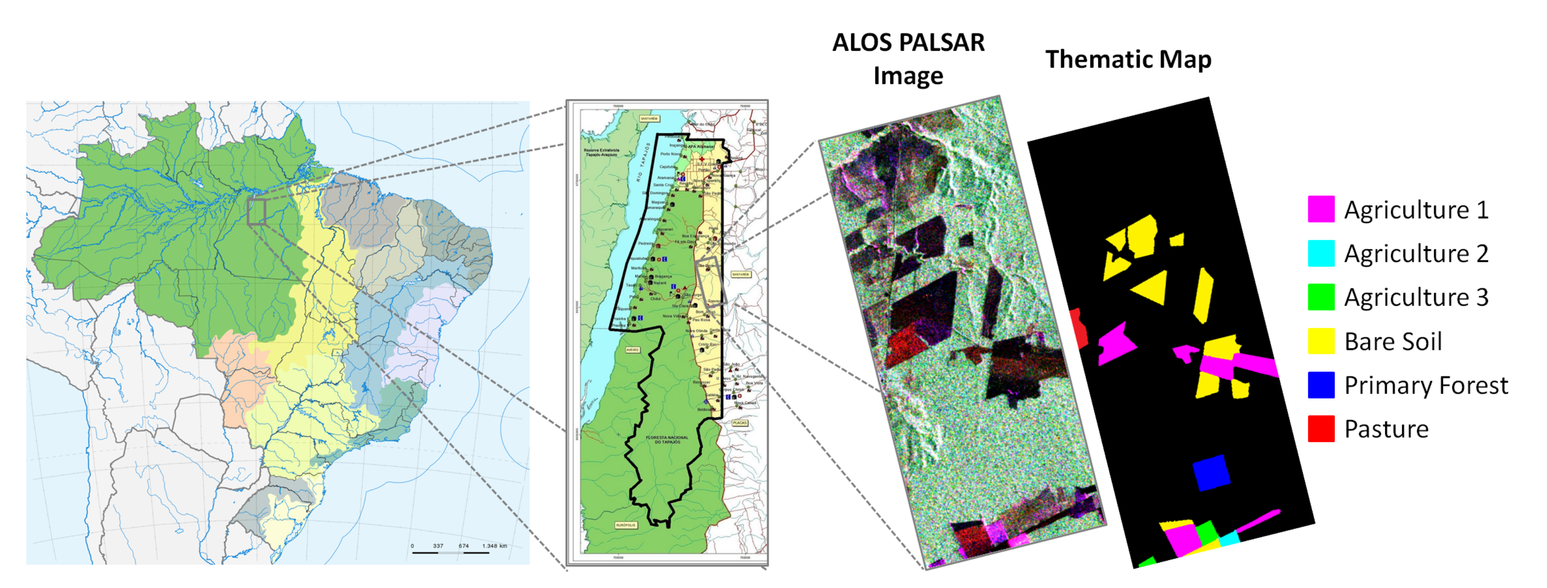
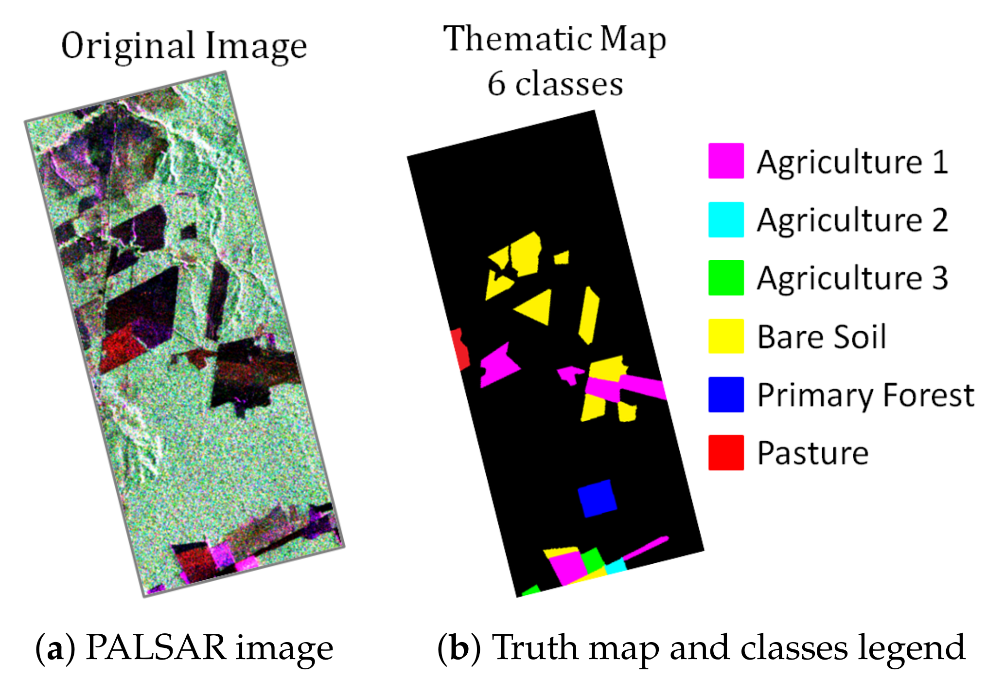
The tested image showed in Figure 10, are from a study area of Tapajós National Forest, located in Belterra, State of Pará, Brazil. This area is considered an important conservation unit in the Brazilian Amazon Forest.
The PolSAR images were obtained by the ALOS PALSAR sensor with approximately 20 m × 20 m spatial resolution, an estimated number of looks equal to 5, and polarization , , and . This image has the classes: Primary Forest, Pasture, Bare Soil, and three types of Agriculture (Agriculture 1, Agriculture 2 and Agriculture 3). Those classes, represented at the Truth map, were identified by a fieldwork campaign conducted by INPE (National Institute for Space Research).
6.2.2. Results
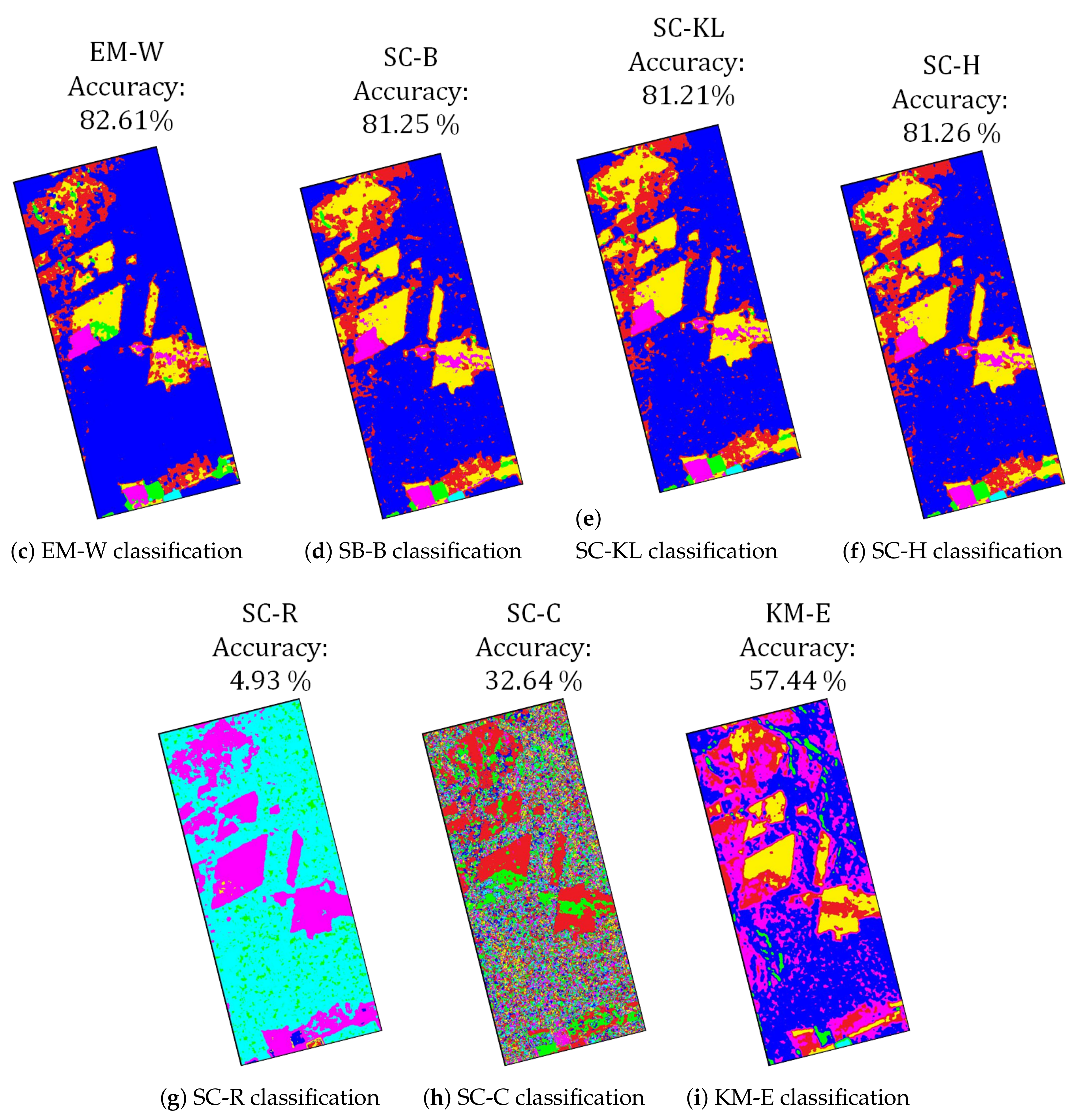
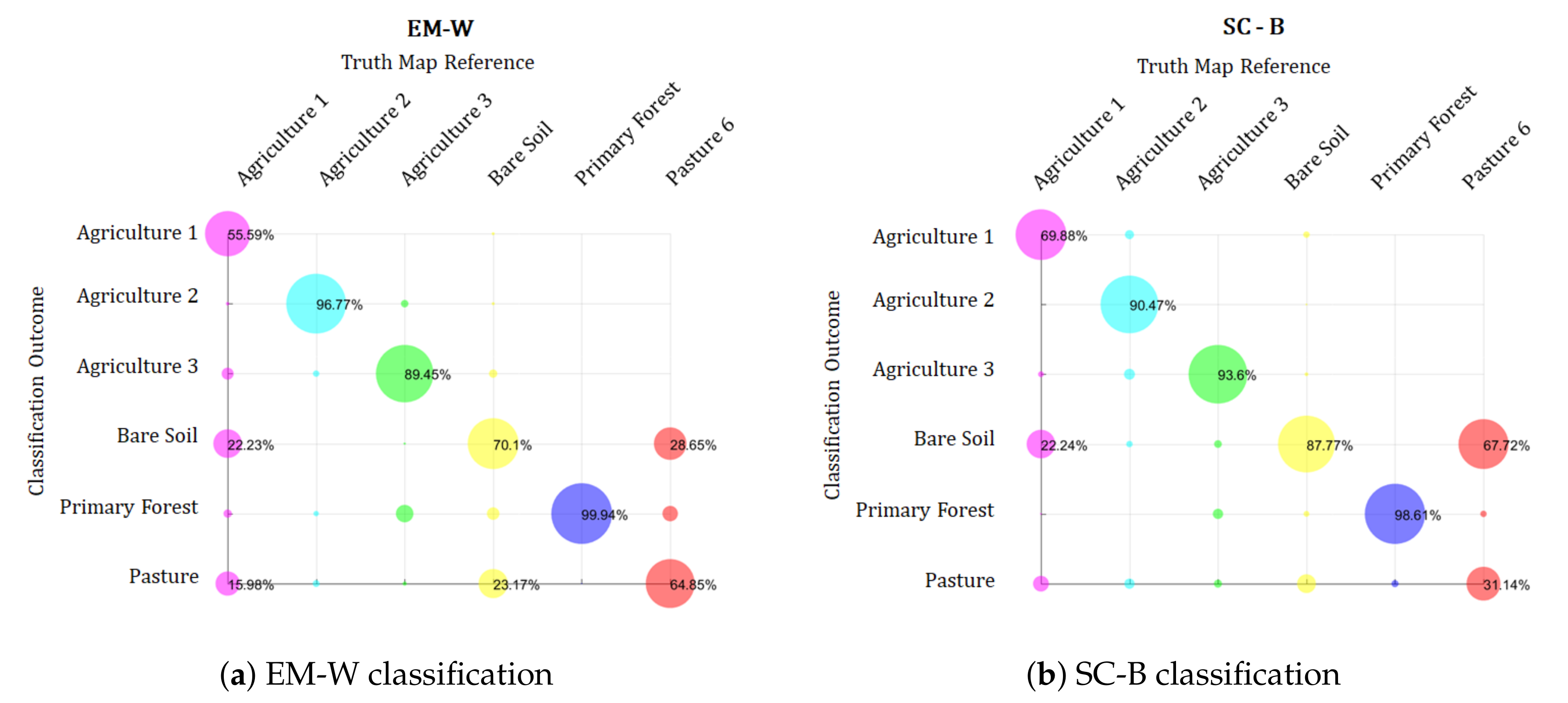
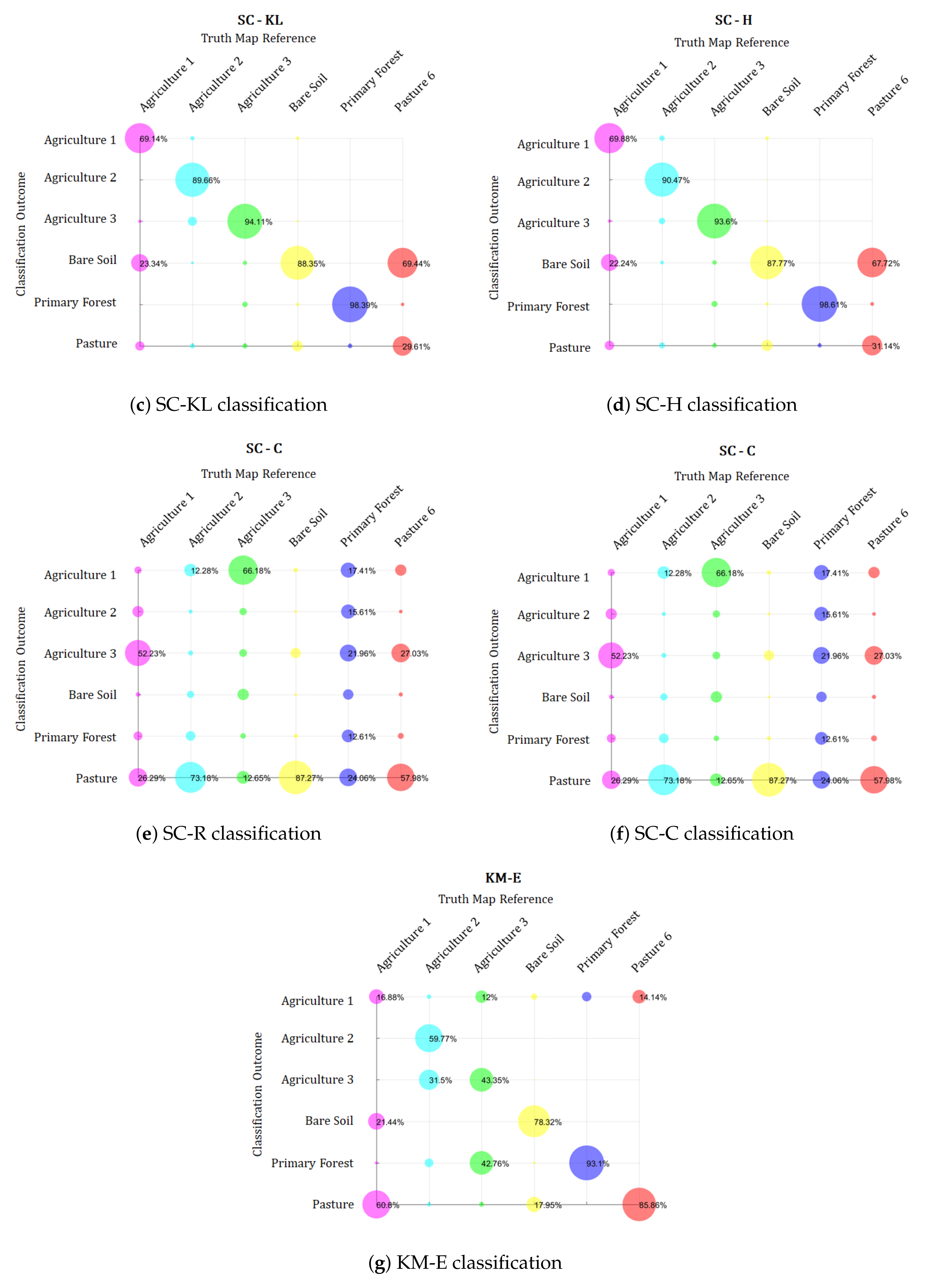
Figure 11 shows the results for PALSAR image and Figure 12 shows the respective confusion matrix bubble graph. We consider only the regions highlighted at the Truth map for initial centroid determination, confusion matrix determination and overall accuracy classification computation. As for simulated images, the overall accuracy was computed by the confusion matrix, where the true values were given by the Truth map, and the outcome values were given by the classification result. Since this image is a not simulated PolSAR image, the speckle is not controlled, therefore more confusion between classes is expected. We can see that the confusion matrices graphs displayed in Figure 12 are more dispersed than the confusion matrices graphs showed in Figure 7.
We applied the seven classification algorithms above-cited on PALSAR image, and compare the results of the classifications against the Truth map. The results show that, as for simulated images, the EM-W (Figure 11c), SC-B (Figure 11d) and SC-H (Figure 11f) had the good overall accuracy results (82.61% and 81.25% and 81.26%, respectively), closed followed by the SC-KL with of overall accuracy. The KM-E algorithm achieved , especially due to misclassifying of Agriculture 3 class, Bare Soil and Pasture. As for simulated images, the worst classification accuracy results came with SC-R and SC-C algorithms, having and , respectively.
7. Discussion
This work uses the statistical information inherent in POLSAR images in order to achieve relatively high classification accuracy, using traditional clustering algorithms, as the EM and K-means. The EM algorithm for the Wishart mixture model has the goal of clustering a set of covariance matrices. The use of Wishart distribution to model PolSAR data leads to the homogeneity assumption, therefore real images, i.e., not simulated, are up to face considerable modeling errors. However, mixture models are powerful tools for irregular distributions approximating when in the presence of hidden data.
The classical K-means uses the Euclidean distance, therefore it assumes that the variance of a given cluster is spherical, indeed this algorithm can be seen as is a special case of Gaussian mixture models. Also, K-means needs linear separability among clusters to correctly distinguish them and has no prior probability for the K clusters, as the EM algorithm. In short, the K-means algorithm fails when dealing with PolSAR data having a low number of looks. To overcome this issue, in this work we used as similarity metric for K-means strategy the stochastic distances, and, since the centroids are not the cluster mean anymore, but the averaged covariance matrix, we named this approach as Stochastic Clustering. We presented five versions of SC, each considering a different stochastic distance, videlicet: Bhattacharyya, Kullback-Leibler, Rényi of order , Hellinger and Chi-square.
In order to evaluate the SC algorithm performance, a Monte Carlo simulation was conducted over seven algorithms: EM-W, SC-B, SC-KL, SC-H, SC-R, SC-C and KM-E. The EM-W showed to have great potential, classifying the homogeneous areas with small errors, for instance, the primary forest class in Figure 11c had of accuracy (Figure 12a). On average, the KM-E algorithm classification results for PolSAR images were underachieving, providing wrongly and noising classification even when the initial centroids were good.
The SC algorithm accuracy performance is highly dependent on the stochastic distance choice. According to [5] the Hellinger distance is the best option when dealing with Wishart distributed data. As expected, the SC-H had one of the best accuracy classification results, closely followed by the SC-B, that can be explained by the close relationship between Bhattacharyya and Hellinger distance. The SC-KL achieved good accuracy results as well. However, SC-R and SC-C had the lowest classification accuracy results, mainly due to numerical instabilities presented by Rényi of order and Chi-square distances. Besides that, the Chi-Square distance also produces higher variation in comparison to the other distances.
The Monte Carlo simulation exposed the dependency of all algorithms upon the correctness of the initial centroids. If the randomly chosen initial parameter is not good, then all the algorithms are likely to terminate at a local maximum or minimum, resulting in the non-optimized estimation, i.e., the algorithm may run a lot of iterations trapped in segments that are away from the global maximum or minimum. Therefore, choosing good candidates for the initial centroids of clustering algorithms is essential for clustering quality and performance. This implies that a better initial guess would make the convergence faster, reducing the amount of time spent in areas away from the global maximum. There are a large number of methods for initial centroids choosing. In [28] a comparative of eight commonly used methods for clustering initialization is presented, for instance, Ball and Hall’s method, Simple Cluster Seeking method, Maximin method, PCA (Principal Component Analysis) method and so on.
Another important factor that directly influences the PolSAR image classification result is the number of looks. Multi-look processing improves the classification results by reducing the speckle noise. However, one main goal of this work is to identify the metrics which are robust to noise interference. The Bhattacharyya, Kullback-Leibler and Hellinger distance proved to be great metrics to class separability. During the Monte Carlo simulation (where the PolSAR images were simulated with 3 looks only) those distances had a consistency overall accuracy, having more than of the result with accuracy higher than .
8. Conclusions
In this work, a Monte Carlo simulation over simulated PolSAR image was performed in order to compare several stochastic distances against the Euclidean distance and the Wishart mixture model. The EM algorithm provides simple iterative solutions for problems where the direct likelihood function optimization is difficult. The use of EM algorithm ally to Wishart distribution allows us to compare random variables viewed as multivariate sample sets, for instance, covariance matrices.
The use of Bhattacharyya, Kullback-Leibler, and Hellinger as similarity metrics on the SC algorithm achieved successful results. The Rényi of order and Chi-square are not indicated to perform classification when the number of looks is small, due to their numerical instabilities, leading to poor accuracy results.
On average, the SC-B and SC-H outperformed the other algorithms. Even though the EM-W can have great classification performance, for a limited number of iteration, on average this algorithm can generate a medium to low accuracy result, very close to KM-E behavior.
In further studies, the influence of the number of looks and the number of iteration shall be considered in Monte Carlo analyses. Also, studies on heterogeneous areas, where more advanced distribution models are required, shall be evaluated.
Author Contributions
N.C.R.L.C. developed the codes in Matlab, designed, conducted and performed all the experiments, helped to design the accuracy assessment and wrote the paper under the supervision of L.S.A.B. and S.J.S.S., L.S.A.B. and S.J.S.S. analyzed the experimental data and the obtained results and helped to design the accuracy assessment. All authors were involved in the paper development, the literature review and the discussion of the results.
Funding
This research received no external funding
Conflicts of Interest
The authors declare no conflict of interest.
References
- Lee, J.S.; Pottier, E. Polarimetric Radar Imaging: From Basics to Applications; CRC Press: Boca Raton, FL, USA, 2009. [Google Scholar]
- Song, H.; Yang, W.; Xu, X.; Liao, M. Unsupervised PolSAR imagery classification based on jensen-bregman logdet divergence. In Proceedings of the 10th European Conference on Synthetic Aperture Radar (EUSAR 2014), Berlin, Germany, 3–5 June 2014; pp. 1–4. [Google Scholar]
- Frery, A.C.; Cintra, R.J.; Nascimento, A.D. Entropy-based statistical analysis of PolSAR data. IEEE Trans. Geosci. Remote Sens. 2012, 51, 3733–3743. [Google Scholar] [CrossRef]
- Silva, W.; Freitas, C.; Sant’Anna, S.; Frery, A.C. PolSAR region classifier based on stochastic distances and hypothesis tests. In Proceedings of the 2012 IEEE International Geoscience and Remote Sensing Symposium, Munich, Germany, 22–27 July 2012; pp. 1473–1476. [Google Scholar]
- Frery, A.C.; Nascimento, A.D.; Cintra, R.J. Analytic expressions for stochastic distances between relaxed complex Wishart distributions. IEEE Trans. Geosci. Remote Sens. 2013, 52, 1213–1226. [Google Scholar] [CrossRef] [Green Version]
- Frery, A.C.; Correia, A.; Rennó, C.D.; Freitas, C.; Jacobo-Berlles, J.; Mejail, M.; Vasconcellos, K.; Sant’anna, S. Models for synthetic aperture radar image analysis. Resenhas (IME-USP) 1999, 4, 45–77. [Google Scholar]
- Gao, G. Statistical modeling of SAR images: A survey. Sensors 2010, 10, 775–795. [Google Scholar] [CrossRef] [PubMed]
- Nascimento, A.D.C.D. Teoria EstatíStica da InformaçãO Para Dados de Radar de Abertura SintéTica Univariados E PolariméTricos. Ph.D. Thesis, Federal University of Pernambuco, Recife, Pernambuco, Brazil, 2012. [Google Scholar]
- Torres, L.; Sant’Anna, S.J.; da Costa Freitas, C.; Frery, A.C. Speckle reduction in polarimetric SAR imagery with stochastic distances and nonlocal means. Pattern Recognit. 2014, 47, 141–157. [Google Scholar] [CrossRef] [Green Version]
- Saldanha, M.F.S. Um Segmentador Multinível Para Imagens SAR PolariméTricas Baseado na DistribuiçãO Wishart. Ph.D. Thesis, National Institute for Space Research, São José dos Campos, São Paulo, Brazil, 2013. [Google Scholar]
- Doulgeris, A.P. An Automatic U-Distribution and Markov Random Field Segmentation Algorithm for PolSAR Images. IEEE Trans. Geosci. Remote Sens. 2014, 53, 1819–1827. [Google Scholar] [CrossRef] [Green Version]
- Doulgeris, A.P.; Eltoft, T. PolSAR image segmentation—Advanced statistical modelling versus simple feature extraction. In Proceedings of the 2014 IEEE Geoscience and Remote Sensing Symposium, Quebec City, QC, Canada, 13–18 July 2014; pp. 1021–1024. [Google Scholar]
- Yang, W.; Liu, Y.; Xia, G.S.; Xu, X. Statistical mid-level features for building-up area extraction from high-resolution PolSAR imagery. Prog. Electromagn. Res. 2012, 132, 233–254. [Google Scholar] [CrossRef]
- Silva, W.B.; Freitas, C.C.; Sant’Anna, S.J.; Frery, A.C. Classification of segments in PolSAR imagery by minimum stochastic distances between Wishart distributions. IEEE J. Sel. Top. Appl. Earth Obs. Remote Sens. 2013, 6, 1263–1273. [Google Scholar] [CrossRef] [Green Version]
- Braga, B.C.; Freitas, C.C.; Sant’Anna, S.J. Multisource classification based on uncertainty maps. In Proceedings of the 2015 IEEE International Geoscience and Remote Sensing Symposium (IGARSS), Milan, Italy, 13–18 July 2015; pp. 1630–1633. [Google Scholar]
- Formont, P.; Pascal, F.; Vasile, G.; Ovarlez, J.P.; Ferro-Famil, L. Statistical classification for heterogeneous polarimetric SAR images. IEEE J. Sel. Top. Signal Process. 2010, 5, 567–576. [Google Scholar] [CrossRef] [Green Version]
- Negri, R.G.; Frery, A.C.; Silva, W.B.; Mendes, T.S.; Dutra, L.V. Region-based classification of PolSAR data using radial basis kernel functions with stochastic distances. Int. J. Digit. Earth 2019, 12, 699–719. [Google Scholar] [CrossRef] [Green Version]
- Deng, X.; López-Martínez, C.; Chen, J.; Han, P. Statistical modeling of polarimetric SAR data: A survey and challenges. Remote Sens. 2017, 9, 348. [Google Scholar] [CrossRef] [Green Version]
- Kullback, S.; Leibler, R.A. On information and sufficiency. Ann. Math. Stat. 1951, 22, 79–86. [Google Scholar] [CrossRef]
- Salicru, M.; Menendez, M.; Morales, D.; Pardo, L. Asymptotic distribution of (h, φ)-entropies. Commun. Stat. Theory Methods 1993, 22, 2015–2031. [Google Scholar] [CrossRef]
- Seghouane, A.K.; Amari, S.I. The AIC criterion and symmetrizing the Kullback–Leibler divergence. IEEE Trans. Neural Netw. 2007, 18, 97–106. [Google Scholar] [CrossRef] [PubMed]
- Wang, Y.-H.; Han, C.-Z. Polsar image segmentation by mean shift clustering in the tensor space. Acta Autom. Sin. 2010, 36, 798–806. [Google Scholar] [CrossRef] [Green Version]
- Pakhira, M.K. A linear time-complexity k-means algorithm using cluster shifting. In Proceedings of the 2014 International Conference on Computational Intelligence and Communication Networks, Bhopal, India, 14–16 November 2014; pp. 1047–1051. [Google Scholar]
- Hidot, S.; Saint-Jean, C. An Expectation–Maximization algorithm for the Wishart mixture model: Application to movement clustering. Pattern Recognit. Lett. 2010, 31, 2318–2324. [Google Scholar] [CrossRef]
- Silva, W.B. Classificação de RegiãO de Imagens Utilizando Teste de HipóTese Baseado em DistâNcias EstocáSticas: AplicaçãO a Dados PolariméTricos. Ph.D. Thesis, National Institute for Space Research São José dos Campos, São Paulo, Brazil, 2013. [Google Scholar]
- Jain, A.K. Data clustering: 50 years beyond K-means. Pattern Recognit. Lett. 2010, 31, 651–666. [Google Scholar] [CrossRef]
- Frery, A.C.; Nascimento, A.D.; Cintra, R.J. Information theory and image understanding: An application to polarimetric SAR imagery. arXiv 2014, arXiv:1402.1876. [Google Scholar]
- Celebi, M.E.; Kingravi, H.A.; Vela, P.A. A comparative study of efficient initialization methods for the k-means clustering algorithm. Expert Syst. Appl. 2013, 40, 200–210. [Google Scholar] [CrossRef] [Green Version]
Figure 1.
Stochastic Clustering algorithm flowchart.

Figure 2.
Expectation Maximization for Wishart Mixture Model flowchart.

Figure 3.
(a) Resolution Cell. (b) Constructive sum of scatters returns. (c) Destructive sum of scatters returns.
Figure 3.
(a) Resolution Cell. (b) Constructive sum of scatters returns. (c) Destructive sum of scatters returns.

Figure 4.
(a) PolSAR image in 1-look, obtained by R99B sensor, used to simulate PolSAR data. (b) The phantom image (c) Simulated Image example, containing 36 segments and 6 classes.
Figure 4.
(a) PolSAR image in 1-look, obtained by R99B sensor, used to simulate PolSAR data. (b) The phantom image (c) Simulated Image example, containing 36 segments and 6 classes.

Figure 5.
Monte Carlo simulation flowchart.

Figure 6.
Simulated image classification result.

Figure 7.
Confusion matrix of the simulated PolSAR image classification results presented in Figure 6.
Figure 7.
Confusion matrix of the simulated PolSAR image classification results presented in Figure 6.


Figure 8.
Classification Accuracy boxplot.

Figure 9.
Accuracy of same Image Classification with different initial centroid.

Figure 10.
Study area of Tapajós National Forest, located in the state of Pará. The PolSAR color composition (, and ) image and the Truth Map image with the spatial distribution of classes.
Figure 10.
Study area of Tapajós National Forest, located in the state of Pará. The PolSAR color composition (, and ) image and the Truth Map image with the spatial distribution of classes.

Figure 11.
The study area of Tapajós National Forest PalSAR image classification results.


Figure 12.
Confusion matrix of the PalSAR image classification results presented in Figure 11.
Figure 12.
Confusion matrix of the PalSAR image classification results presented in Figure 11.


Table 1.
Average complex covariance matrix samples calculated from five samples of each class taken from R99B Sensor Image.
Table 1.
Average complex covariance matrix samples calculated from five samples of each class taken from R99B Sensor Image.
| Class Name | Covariance Matrix |
|---|---|
| Class 1 | |
| Class 2 | |
| Class 3 | |
| Class 4 | |
| Class 5 | |
| Class 6 |
Table 2.
Algorithms Accuracy (%).
| EM-W | SC-B | SC-KL | SC-H | SC-R | SC-C | KM-E | |
|---|---|---|---|---|---|---|---|
| Average Accuracy | 54.34 | 72.21 | 70.91 | 72.29 | 35.22 | 41.72 | 57.99 |
| Average STD | 15.98 | 17.05 | 16.79 | 17.06 | 6.15 | 5.22 | 10.48 |
Table 3.
Algorithms Accuracy (%).
| EM-W | SC-B | SC-KL | SC-H | SC-R | SC-C | KM-E | |
|---|---|---|---|---|---|---|---|
| S01 | 36.41 | 48.13 | 31.20 | 48.23 | 41.36 | 40.14 | 47.37 |
| S02 | 36.06 | 48.02 | 34.45 | 48.12 | 45.46 | 30.74 | 45.72 |
| S03 | 49.03 | 64.26 | 65.49 | 63.26 | 46.86 | 33.95 | 59.17 |
| S04 | 65.30 | 58.68 | 60.62 | 58.78 | 30.35 | 35.77 | 56.67 |
| S05 | 55.72 | 51.21 | 54.75 | 51.31 | 45.23 | 31.81 | 47.20 |
| S06 | 95.29 | 94.67 | 93.91 | 94.77 | 47.79 | 44.15 | 62.97 |
Table 4.
Algorthms execution time (s).
| EM-W | SC-B | SC-KL | SC-H | SC-R | SC-C | KM-E | |
|---|---|---|---|---|---|---|---|
| Time | 30.35 | 22.93 | 24.47 | 24.07 | 23.95 | 26.522 | 21.52 |
© 2019 by the authors. Licensee MDPI, Basel, Switzerland. This article is an open access article distributed under the terms and conditions of the Creative Commons Attribution (CC BY) license (http://creativecommons.org/licenses/by/4.0/).
Share and Cite
MDPI and ACS Style
Carvalho, N.C.R.L.; Sant’Anna Bins, L.; Siqueira Sant’Anna, S.J. Analysis of Stochastic Distances and Wishart Mixture Models Applied on PolSAR Images. Remote Sens. 2019, 11, 2994. https://doi.org/10.3390/rs11242994
AMA Style
Carvalho NCRL, Sant’Anna Bins L, Siqueira Sant’Anna SJ. Analysis of Stochastic Distances and Wishart Mixture Models Applied on PolSAR Images. Remote Sensing. 2019; 11(24):2994. https://doi.org/10.3390/rs11242994
Chicago/Turabian StyleCarvalho, Naiallen Carolyne Rodrigues Lima, Leonardo Sant’Anna Bins, and Sidnei João Siqueira Sant’Anna. 2019. "Analysis of Stochastic Distances and Wishart Mixture Models Applied on PolSAR Images" Remote Sensing 11, no. 24: 2994. https://doi.org/10.3390/rs11242994
Note that from the first issue of 2016, this journal uses article numbers instead of page numbers. See further details here.