Remote Sensing Retrieval of Turbidity in Alpine Rivers based on high Spatial Resolution Satellites

Abstract

Turbidity, relating to underwater light attenuation, is an important optical parameter for water quality evaluation. Satellite estimation of turbidity in alpine rivers is challenging for common ocean color retrieval models due to the differences in optical properties of the water bodies. In this study, we present a simple two-band semi-analytical turbidity (2BSAT) retrieval model for estimating turbidity in five alpine rivers with varying turbidity from 1.01 to 284 NTU. The model was calibrated and validated, respectively, while using one calibration dataset that was obtained from the Three Parallel Rivers basin and two independent validation datasets that were obtained from the Kaidu River basin and the Yarlung Zangbo River basin. The results show that the model has excellent performance in deriving turbidity in alpine rivers. We verified the consistency of the simulated reflectance and satellite-based reflectance and calibrated the 2BSAT model for the specified bands of high spatial resolution satellites in order to achieve the goal of remote sensing monitoring. It is concluded that the model can be used for the quantitative monitoring of turbidity in alpine rivers using satellite images. Based on the model, we used the Sentinel-2 images from one year to identify the seasonal patterns of turbidity of five alpine rivers and the Landsat series images from 1989 to 2018 to analyze the turbidity variation trends of these rivers. The results indicate that the turbidity of these alpine rivers usually presents the highest level in summer, followed by spring and autumn, and the lowest in winter. Meanwhile, the variation trends of turbidity over the past 30 years present distinctly different characteristics in the five rivers.

1. Introduction

Rapid and accurate remote retrieval of water quality parameters is essential for evaluating the aquatic environment and water security in largescale inland waters. Turbidity (TU) is the most intuitive expression of water quality, which directly affects the attenuation of light in the water, thereby affecting photosynthetic activities and the primary productivity of phytoplankton in the water [1,2,3]. Furthermore, turbidity is also an indicator of the concentration of the total suspended matter (TSM), which is the main factor affecting the turbidity level in water. It is possible to interpret the complex hydrological processes of TSM through identifying the lager-scale spatiotemporal dynamics of turbidity, such as migration, sedimentation, and resuspension [4]. Thus, knowledge of the turbidity patterns and dynamic characteristics is significant in aquatic environmental protection and water resource management.

Known as the “Asian Water Tower”, the Tibetan Plateau feeds many large rivers in Asia, including the Yellow River, the Yangtze River, the Yarlung Zangbo River (YZR), the Tarim River, the Lancang-Mekong River, the Salween River, the Indus River, and so on. The abundant reserve of water resources provides access to more than 1.5 billion people in 10 countries [5]. However, the alpine ecosystem of the Tibetan Plateau, especially the river ecosystem, is highly sensitive to climate change and human activities [6]. Thus, the unique geographical and climatic conditions of the Tibetan Plateau have made the water environment the focus of plateau ecology and environmental research. The YZR is the highest river in the world being located in the south of the plateau. In addition, the YZR basin is the most important economic zone in the Tibet Autonomous Region. The Three Parallel Rivers (TPR) is composed of the Jinsha River (JSR), Lancang River (LCR), and Nujiang River (NJR), and it is on the southeastern edge of the Tibetan Plateau. Under the impact of neotectonic movement, the three rivers form a rare and spectacular natural landscape, the “Three Rivers Parallel” [7]. Abundant water resources guarantee the biodiversity of the basin. In addition, the Kaidu River (KDR) is an important plateau inland river in the Xinjiang Autonomous Region and it has always been the ecological source for the southern Xinjiang oasis. The fragile ecological environment of these alpine rivers brings about severe challenges for water quality monitoring and protection, especially in the context of intense human activities. For example, agriculture production, hydropower projects, mineral excavation, and tourism development impact the original ecology of river aquatic environment. Thus, the water quality of these alpine rivers is considered to be a critical issue in ecological environmental protection.

River ecosystems have received relatively little attention in the monitoring of water turbidity when compared with large, open waters, such as oceans and coastal areas, or relatively quiescent or slow-flowing regional waters, such as estuaries, lakes, and reservoirs. This is because river systems have more obvious dynamics characteristics over a short time, and the optical properties are more complex under the influences of quick hydrodynamics, strong climate change events, and anthropogenic activities. Therefore, identifying the turbidity pattern and spatiotemporal variations in complex river environment requires non-traditional approaches. Remote sensing technology has been widely used in the extraction of various water quality parameters, including turbidity in large areas by virtue of its cyclical, large-scale, rapid synchronous monitoring [8]. However, it is still difficult to monitor river turbidity, because the relatively narrow river channel leads to the existence of fewer image pixels in the transverse direction of the river. Fortunately, the successful development of advanced high spatial resolution and hyperspectral sensors expands the application of remote sensing technology in the monitoring of the water quality in narrow rivers [9,10]. The combination of remote sensing imagery and the river water spectrum can provide favorable conditions for comprehensively revealing turbidity changes in a regional water environment from a more macroscopic perspective. Identifying landslide origins and the spatial distribution of turbidity are very conducive for monitoring the affected range and the extent of damage to water quality in real time, especially in some disaster-prone watersheds.

As of now, various turbidity models for ocean, coastal, and lake water quality monitoring have been developed, including statistical, semi-analytical, and physical models, as well as some special retrieval models, such as neural networks [11,12,13,14]. Based on these models, numerous water body studies have estimated the turbidity of some oceans and large lakes [15,16,17,18]. However, it should be mentioned that the hydrological characteristics of rivers, especially alpine rivers, are vastly different from those of oceans and lakes [19]. Models that are based on optical properties of latter cannot be directly applied to river systems. In addition, statistical models are mainly based on the statistical regression relationship between Apparent Optical Properties (AOPs) and the measured turbidity. Such models are only applicable to waters with a single optical property. Physical models that are based on the radiation transfer theory aimed at solving the reflectance model with water constituents are rather complex, and the detailed construction of its theory is still immature [20,21]. Moreover, it is difficult to obtain the optical property information of rivers in the alpine environment. Semi-analytical models aim to establish the relationship between the Inherent Optical Properties (IOPs) of water and the measured turbidity by relating the AOPs to IOPs [22,23,24,25]. In practice, some approximate empirical hypotheses are always integrated into semi-analytic models to simplify the operation process. Therefore, semi-analytic models are still the most effective method in current water quality monitoring.

In addition, it is proved that there is a strong linear correlation between turbidity and TSM [26,27,28,29]. An increase of the TSM concentration in the water enhances the attenuation effect of light, which results in an increase in the turbidity of the water. Many studies quantify turbidity by retrieving the concentration of TSM by means of the empirical relationship of TU and TSM [15,30]. This indirect approach is easy to achieve, because the spectral characteristics of the latter are obvious. However, the remote sensing reflectance might be saturation at certain levels of TSM [31]. Thus, it still remains a challenge that directly using the relationship of remote sensing reflectance and TSM to estimate turbidity in alpine rivers.

In this study, a two-band semi-analytical TU retrieval model (2BSAT) was proposed for retrieving TU from satellite images in five alpine rivers in China. The main goals of the study are as follows: (a) to verify the performance accuracy of four existing models for retrieving TU in river system and compare the accuracy of the four models and 2BSAT; (b) to identify the spatial distribution characteristics and the seasonal patterns of river turbidity while using Sentinel-2 images with high spatiotemporal resolution and analyze the long-term changes of river turbidity using Landsat series images from 1990 to 2018; and, (c) to briefly discuss the factors affecting turbidity in rivers.

2. Materials and Methods

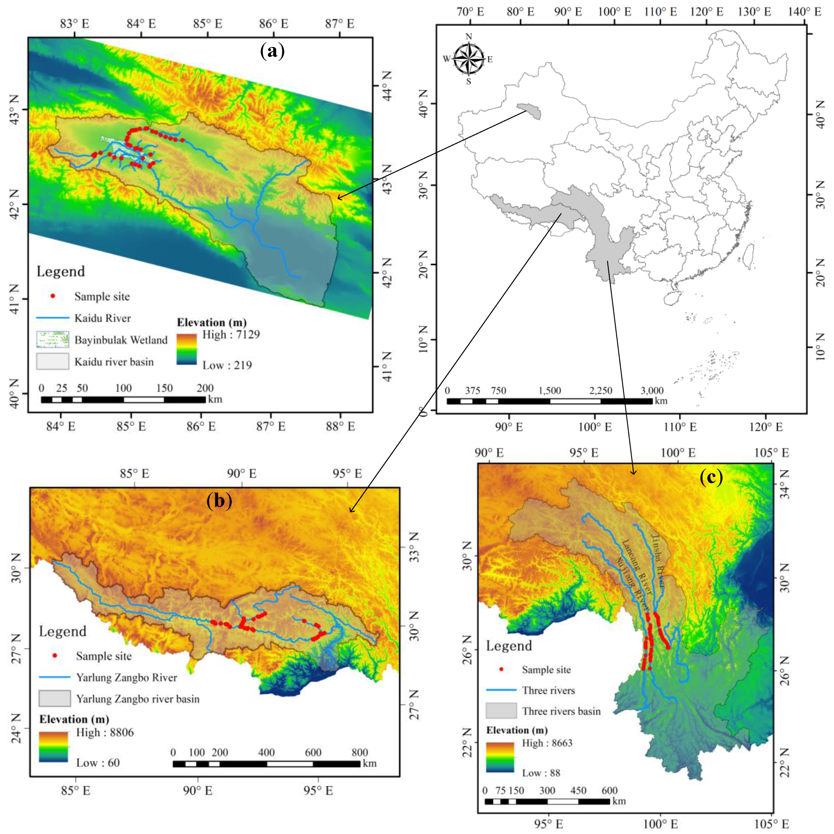
2.1. Study Area

The study area consisted of the Kaidu River basin, the Yarlung Zangbo River basin, and the Three Parallel Rivers basin (JSR, LCR, and NJR). These rivers are located in western and southwestern China (Figure 1).

The Kaidu River basin is located in the hinterland of the Xinjiang Autonomous Region (Figure 1a). The KDR flows through the Bayanbulak Wetland at an altitude of over 2500 m. The water bodies in the core area of the wetland present the original water quality state, which is because the marsh area has been isolated from the influence of human activities, while some small lakes and tributaries located on the edge of the wetland have been seriously disturbed by animal husbandry and tourism.

The Yarlung Zangbo River basin is located in the southern part of the Tibetan Plateau (Figure 1b). The YZR is the highest river in the world and flows through China, India, and Bangladesh. In addition, it is the main freshwater source and water-vapor channel for the Tibetan Plateau. Our study area in the basin is located in the middle reaches of the YZR, with an average elevation of over 3000 m, including two major tributaries of the Lhasa River and the Niyang River. The region is densely populated with active industrial and agricultural production and convenient transportation. It is also the most prosperous region of the political, economic, and multiethnic culture of the Tibet Autonomous Region.

The Three Parallel Rivers basin is located at the southeast edge of Tibetan Plateau (Figure 1c). The elevation gradually decreases from the Tibetan Plateau in the northwest to the Yunnan-Guizhou Plateau in the southeast. Active neotectonic movements make mountains and rivers interphase distribution in the area. The three rivers of the JSR, LCR, and NJR, which originate from the Tibetan Plateau, flow parallelly more than 170 km from north to south in Yunnan Province. In recent years, the construction of the Yunnan-Tibet and Sichuan-Tibet roads, railways, and factories along rivers has severely affected the water quality of these rivers.

2.2. Data Collection

In the above three watersheds, we conducted three field investigations and then collected 40 samples (Figure 1b) in YZR during 21–26 September 2016, 38 samples (Figure 1a) in KDR during 16–20 July 2018, and 70 samples (Figure 1c) in TPR (30 in JSR, 28 in LCR, and 12 in NJR) during 3–12 November 2018.

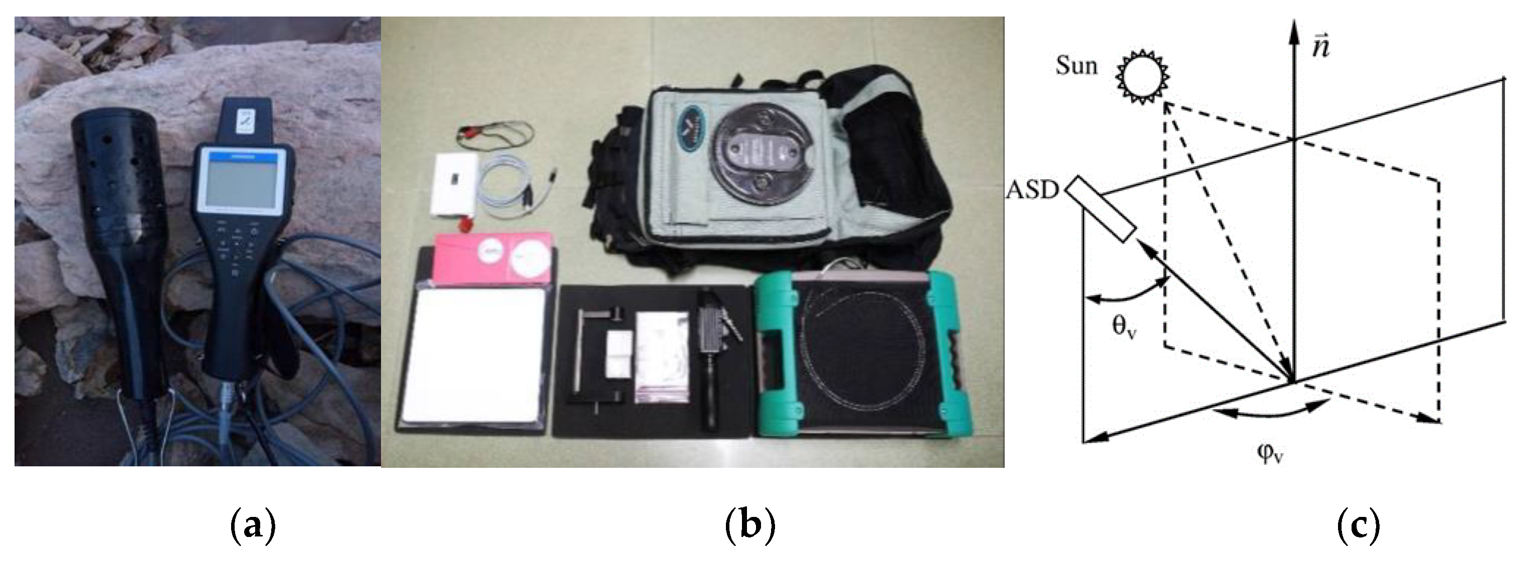
2.2.1. In Situ Measurements

At each sampling site, the HORIBA multi-parameter water quality meter U-50 (Figure 2a) was deployed to measure the hydrochemistry parameters of water, including turbidity, temperature, PH, chemical oxygen demand, and water depth, and so on. These parameters were measured in quintuplicates and they were averaged as effective measurements.

The water remote sensing reflectance ($R_{rs}\left(\lambda \right)$) between 350 and 2500nm was synchronously measured with the ASD Field Spectroradiometer (Figure 2b) when collecting water samples. The spectrometer has a spectral resolution of 1nm in the measurement range. We adopted the above-surface observation method (Figure 2c), and the method that was designed by the scientific measurement angle can effectively avoid the effects of direct sunlight, surrounding objects, and measurement environment.

Field spectrum measurements were performed under consistently bright sunny weather conditions. The optimization of ASD required taking a reference while using a standard reflecting reference plate before each measurement. The following three optical physical parameters were measured: downwelling irradiance above the water surface ($E_d\left(0^{+}\right)$), total upwelling radiance from water ($L\left(\lambda \right)$), and downwelling sky radiance ($L_p\left(\lambda \right)$), where $E_d\left(0^{+}\right)$ was obtained by measuring the reflected radiance $L_G\left(\lambda \right)$ of the standard reference plate. All of these optical physical parameters were measured 10 times in succession at each sampling site and then averaged as effective values to calculate $R_{rs}\left(\lambda \right)$ after removing the outliers.

$$R_{rs}\left(\lambda \right)=\frac{L_w\left(\lambda \right)}{E_d\left(0^{+}\right)}=\frac{L\left(\lambda \right)-\rho \times L_P\left(\lambda \right)}{L_G\left(\lambda \right)\times \pi /{\rho }_b}\times 100\%$$

(1)

where $L_w\left(\lambda \right)$ represents the water-leaving radiance calculated from $L\left(\lambda \right)$ by means of atmospheric correction procedure; $\rho$ represents the reflection coefficient of the air-water interface to the sky light, which is related to the solar zenith angle, wind speed, observation geometry, and the surface roughness, and so on; and, ${\rho }_b$ represents the corrected reflection coefficient of the standard reference plate.

2.2.2. Water Sampling and Laboratory Analysis

In the middle reaches of the YZR and the parallel reaches of the TPR, we collected water samples every 10 km along the mainstream and added samples at the entrances of some major tributaries. In the Bayanbulak Wetland, we not only sampled the mainstream of the Kaidu River, but also water samples from calm, small lakes in the wetlands. The location and elevation of these sample sites were recorded while using a handheld GPS.

The water samples were collected from optically deep-water areas to avoid the effects of water-bottom reflectance. We measured Chlorophyll-a (Chl-a), Total Organic Carbon (TOC), Dissolved organic carbon (DOC), and TU in the laboratory after the field campaign. One liter of river water was required for each sample and was stored in a dark, refrigerated environment. Chl-a was extracted while using methanol at 4℃ for 24h in a dark environment, and the concentrations were determined by fluorometric analysis [33]. The TOC and DOC concentrations were measured while using a Total Organic Carbon analyzer (Siever 900) that was equipped with an autosampler. The TU of sample water was determined by spectrophotometry method.

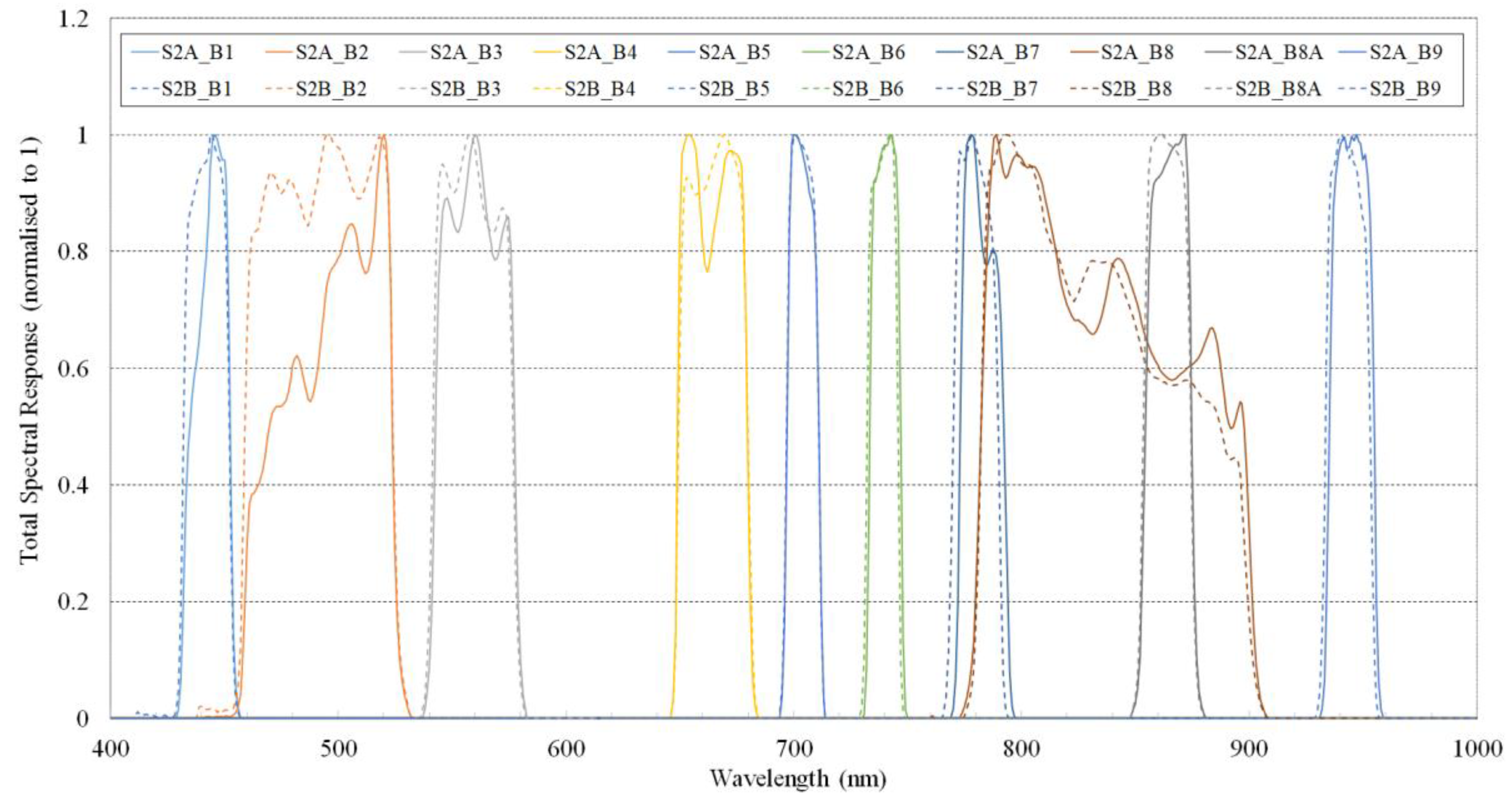
2.2.3. Satellite Observation

As a part of the ESA Copernicus Earth Environment Monitoring Project, Sentinel-2 is a system that is composed of two polar-orbiting satellites, 2A and 2B, which were launched on 23 June 2015 and 7 March 2017, respectively. Each of the two satellites is equipped with a Multispectral Instrument (MSI) with 13 spectral bands that range from the visible and near-infrared (NIR) to the short-wave infrared [34]. The MSI has three types of spatial resolutions (10, 20, and 60 m), depending on different spectral bands (

Table 1. Channel’s parameters of the Sentinal-2 Multispectral Instrument (MSI) sensor.

Band	Central Wavelength (nm)	Band Range (nm)	GSD 1 (m)
B1-Coastal aerosol	443	430–457	60
B2-Blue	490	440–538	10
B3-Green	560	537–582	10
B4-Red	665	646–684	10
B5-Vegetation Red Edge	705	694–713	20
B6-Vegetation Red Edge	740	731–749	20
B7-Vegetation Red Edge	783	769–797	20
B8-NIR	842	760–908	10
B8A-Narrow NIR	865	848–881	20
B9-Water Vapor	945	932–958	60
B10-SWIR-Cirrus	1375	1337–1412	60
B11-SWIR	1610	1539–1682	20
B12-SWIR	2190	2078–2320	20

¹ GSD is Ground Sample Distance, also called spatial resolution.

). The swath of Sentinel-2 images is 290km, and the revisit time of a single satellite is 10 days, which can reduce to five days when the two satellites observe the same area. Therefore, Sentinel-2 images are decent data sources for river water quality monitoring.

The Sentinel-2 data for this study were downloaded from the ESA Copernicus Open Access HUB (https://scihub.copernicus.eu/), and images atmospheric correction were implemented by while using the specialized Sen2Cor (version 2.8) plugin released by the ESA. We used Sentinel-2 images that were ingested from the autumn of 2018 to the summer of 2019 to analyze the spatial distributions and seasonal patterns of turbidity in each alpine river.

Landsat series data is one of the earliest data sources for water environmental monitoring. Although the terrestrial satellite channel setup is not for marine applications, it has been the most widely used data source for water body remote sensing. This study used the Landsat series data to prolong the time series of water turbidity monitoring, including Landsat TM, ETM+, and OLI, because of the good consistency between the Sentinel-2 series and the Landsat series data [17] (

Table 2. Channel’s parameters of Landsat series sensors.

Landasat-8 OLI			Landasat-7 ETM+			Landasat-5 TM
Band	Range (nm)	GSD (m)	Band	Range (nm)	GSD (m)	Band	Range (nm)	GSD (m)
B1-Coastal	433–453	30
B2-Blue	450–515	30	B1-Blue	450–525	30	B1-Blue	450–520	30
B3-Green	525–660	30	B2-Green	525–605	30	B2-Green	520–600	30
B4-Red	630–680	30	B3-Red	630–690	30	B3-Red	630–690	30
B5-NIR	845–885	30	B4-NIR	750–900	30	B4-NIR	760–900	30
B6-SWIR1	1560–1660	30	B5-SWIR	1550–1750	30	B5-SWIR	1550–1750	30
B7-SWIR2	2100–2300	30	B6-LWIR	10,400–12,500	60	B6-LWIR	10,400–12,500	120
B8-Pan	500–680	15	B7-SWIR	2090–2350	30	B7-SWIR	2080–2350	30
B9-Cirrus	1360–1390	30	B8-Pan	520–900	15

). The number of satellite images used in this study is showed in

Table 3. Statistical description of satellite images used for retrieving Turbidity (TU).

	TPR		KDR		YZR
	Path/Row	Number	Path/Row	Number	Path/Row	Number
Sentinel-2A/B (2018.9–2019.8)	T47/RMM, T47/RNM, T47/RML, T47/RNL, T47/RMK, T47/RNK, T47/RMJ, T47/RNJ	106	T44/TQN	45	T46/RBT, T46/RCT	64
Landsat-5/7/8 (1989–2018)	132/41, 132/42	418	144/30, 145/30	372	138/40	335

.

$R_{rs}\left(\lambda \right)$ weighted by the sensor channel response function (Figure 3) was simulated to the equivalent integral band $R_{eq}\left(\lambda \right)$ by using relation (2) in order to ensure that the field-measured spectrum is comparable to the reflectance obtained by the Sentinel-2 MSI sensor. Equivalent multispectral bands were applied for further analysis.

$$R_{eq}\left(\lambda \right)=\frac{{{\displaystyle \int }}_{{\lambda }_{min}}^{{\lambda }_{max}}{F}_0\left(\lambda \right)R_{rs}\left(\lambda \right)f\left(\lambda \right)d\lambda }{{{\displaystyle \int }}_{{\lambda }_{min}}^{{\lambda }_{max}}{F}_0\left(\lambda \right)f\left(\lambda \right)d\lambda }$$

(2)

where ${\lambda }_{min}$ and ${\lambda }_{max}$ are the bands at the beginning and end of the integration, respectively, corresponding to the shortest and longest wavelengths of each multispectral band. $f\left(\lambda \right)$ represents the spectral response function of a certain band of the sensor. $F_0\left(\lambda \right)$ represents the solar irradiance outside the atmosphere at a certain band.

2.3. Turbidity Model Development

In Section 2.2.1, $R_{rs}\left(\lambda \right)$ is defined as the ratio of the water-leaving radiance $L_w\left(\lambda \right)$ to the downwelling irradiance above the water surface $E_d\left(0^{+}\right)$. The two optical physical parameters are both AOPs. Actually, in a homogeneous water body, $R_{rs}\left(\lambda \right)$ can also be described while using the IOP parameters, namely total absorption and backscattering coefficients, in terms of the subsurface remote sensing reflectance $r_{rs}\left(\lambda \right)$ [22,36,37], as relation (3).

$$R_{rs}\left(\lambda \right)\propto r_{rs}\left(\lambda \right)=\frac{f}{Q}\frac{b_{bt}\left(\lambda \right)}{a_t\left(\lambda \right)+b_{bt}\left(\lambda \right)}$$

(3)

where $f/Q$ is a factor dependent on the Sun, the viewing geometry, and the volume scattering function of water. $a_t\left(\lambda \right)$ is the total absorption coefficient of all the material components in the water, as relation (4), where $a_w\left(\lambda \right)$, $a_{ph}\left(\lambda \right)$, $a_{NAP}\left(\lambda \right)$, and $a_{CDOM}\left(\lambda \right)$ are the absorption coefficients for pure water, phytoplankton, NAP, and colored dissolved organic matter (CDOM), respectively. $b_{bt}\left(\lambda \right)$ is the total backscattering coefficient that is composed of $b_{bw}\left(\lambda \right)$, $b_{b,ph}\left(\lambda \right)$, and $b_{b,NAP}\left(\lambda \right)$, which correspond with the above water components, as relation (5). In the study, $b_{b,ph}\left(\lambda \right)$ and $b_{b,NAP}\left(\lambda \right)$ are merged into the particle backscattering coefficient $b_{b,p}\left(\lambda \right)$. The purpose of this model is to estimate $b_{b,p}\left(\lambda \right)$ because of its tight relationship with water turbidity [38].

$$a_t\left(\lambda \right)=a_{ph}\left(\lambda \right)+a_{NAP}\left(\lambda \right)+a_{CDOM}\left(\lambda \right)+a_w\left(\lambda \right)$$

(4)

$$b_{bt}\left(\lambda \right)=b_{b,ph}\left(\lambda \right)+b_{b,NAP}\left(\lambda \right)+b_{b,w}\left(\lambda \right)=b_{b,p}\left(\lambda \right)+b_{b,w}\left(\lambda \right)$$

(5)

We used the difference of the reciprocal of $R_{rs}\left(\lambda \right)$ at two neighboring bands to isolate $b_{b,p}\left(\lambda \right)$ from $R_{rs}\left(\lambda \right)$ while referring to the structure of some two-band water quality parameter retrieval models in existing literature [32,39,40,41], as relations (6) and (7).

$$R_{rs}{}^{-1}\left(\lambda \right)\propto \frac{Q}{f}\frac{a_{ph}\left(\lambda \right)+a_{NAP}\left(\lambda \right)+a_{CDOM}\left(\lambda \right)+a_w\left(\lambda \right)+b_{bt}\left(\lambda \right)}{b_{bt}\left(\lambda \right)}$$

(6)

$$R_{rs}{}^{-1}\left({\lambda }_1\right)-R_{rs}{}^{-1}\left({\lambda }_2\right)\propto \frac{Q}{f}\frac{a_w\left({\lambda }_1\right)-a_w\left({\lambda }_2\right)}{b_{bt}\left({\lambda }_1\right)}$$

(7)

Firstly, $f/Q$ is assumed to be spectrally invariant in a narrow band range when the in-water zenith and azimuth viewing angles have not changed significantly. At longer wavelengths, like the NIR band, the absorption coefficients of NAP and CDOM appear to exponentially decrease to a low level [41,42,43,44]. $a_{ph}\left(\lambda \right)$ is negligible in comparison with $a_{NAP}\left(\lambda \right)$ in a water body with suspended particles as the main constituent [45]. In addition, the total spectral backscattering coefficient $b_{bt}\left(\lambda \right)$ can be assumed invariant at longer wavelengths (650~900nm) [37,46]. Thereby, based on the above several assumptions, $a_{ph}\left(\lambda \right)$, $a_{NAP}\left(\lambda \right)$, $a_{CDOM}\left(\lambda \right)$, and $b_{bt}\left(\lambda \right)$ at ${\lambda }_1$ and ${\lambda }_2$ can be removed from the numerator in relation (6) by the difference of the reciprocal. When the absorption coefficient and backscattering coefficient of pure water are known [47], we finally obtain

$$\mathrm{TU}\propto b_{b,p}\left({\lambda }_1\right)\propto {\left[R_{rs}{}^{-1}\left({\lambda }_1\right)-R_{rs}{}^{-1}\left({\lambda }_2\right)\right]}^{-1}$$

(8)

By selecting two appropriate spectral bands, ${\lambda }_1$ and ${\lambda }_2$, it appears to isolate the $b_{bt}\left({\lambda }_1\right)$ from the $R_{rs}\left(\lambda \right)$. In this study, we adopted a stepwise ergodic technique that was based on linear regressions from least-squares method to determine the approximate positions of ${\lambda }_1$ and ${\lambda }_2$ [37].

2.4. Accuracy Assessment

In this study, the accuracy of the turbidity model was evaluated by comparing the predicted and measured turbidity. The comparison was expressed in terms of root mean square error (RMSE), mean absolute error (MAE), mean relative error (MRE), and coefficient of determination (R²). The above evaluation indexes are computed, as follows:

$$R^2=1-\frac{{{\displaystyle \sum }}_{i=1}^n{\left(x_{obs,i}-x_{mod,i}\right)}^2}{{{\displaystyle \sum }}_{i=1}^n{\left(x_{obs,i}-{\overline{x}}_{obs,i}\right)}^2}$$

(9)

$$RMSE=\sqrt{\frac{{{\displaystyle \sum }}_{i=1}^n{\left(x_{mod,i}-x_{obs,i}\right)}^2}{n}}$$

(10)

$$MAE=\frac{1}{n}{{\displaystyle \sum }}_{i=1}^n(\left|x_{mod,i}-x_{obs,i}\right|)$$

(11)

$$MRE=\frac{1}{n}{{\displaystyle \sum }}_{i=1}^n(\left|\frac{x_{mod,i}-x_{obs,i}}{x_{obs,i}}\right|)\times 100\%$$

(12)

where $n$ is the number of observations, $x_{obs,i}$ is the observed value of TU, ${\overline{x}}_{obs,i}$ is the average of the observed values, and $x_{mod,i}$ is the predicted value of TU.

3. Results

3.1. Bio-optical Properties of the River Waters

The statistical values of water quality parameters of the five inland rivers, including TU, Chl-a, TOC, and DOC, are shown in

Table 4. Descriptive statistics of water quality parameters in the five rivers. Minimum, Maximum, Mean, Standard Deviation (Std), Coefficient of Variation (CV), and sample number are indicated.

River	Parameter	Min	Max	Mean	Std	CV	Number
YZR	TU(NTU)	2.00	205.00	73.48	54.06	0.74	40
	TOC(mg L−1)	0.61	3.82	1.33	0.55	0.41	40
KDR	Chl-a(mg m−3)	2.53	8.72	4.29	1.65	0.39	38
	TU(NTU)	1.01	75.28	25.77	24.84	0.96	38
	TOC(mg L−1)	0.80	30.13	8.63	7.63	0.88	38
JSR	TU(NTU)	9.59	284.00	208.19	49.90	0.24	30
	TOC(mg L−1)	2.01	4.28	3.84	0.44	0.11	30
	DOC(mg L−1)	1.97	4.08	3.59	0.35	0.10	30
LCR	TU(NTU)	1.64	161.50	51.32	39.04	0.76	28
	TOC(mg L−1)	3.67	4.34	3.97	0.17	0.04	28
	DOC(mg L−1)	2.82	3.95	3.57	0.22	0.06	28
NJR	TU(NTU)	59.00	86.20	67.15	7.09	0.11	12
	TOC(mg L−1)	3.37	4.07	3.61	0.22	0.06	12
	DOC(mg L−1)	2.79	3.13	2.96	0.09	0.03	12

. Turbidity was measured at 148 sample sites in the five rivers and varied over two orders of magnitude from 1.01 NTU up to an extreme 284 NTU. Among the five rivers, the average turbidity of the JSR was the highest, peaking at 208.19 NTU, followed by YZR, NJR, LCR, and the lowest in KDR. These rivers contain extremely turbid water, like JSR, and freshwater, like KDR. We found that there was a good consistency between the two data sources by comparing the turbidity values that were measured by field water quality U-50 m and laboratory analysis. Then, the average of the two data sources was accepted for the following analysis in order to more accurately reflect the actual turbidity of the five rivers.

The concentration of Chl-a in the river water of the both basins was so low that it exceeded the minimum detection limit of the instrument, which indicated a low biomass of phytoplankton in these rivers, because of the alpine climate and geomorphological features of YZR and TPR. In addition, the average concentration of the two parameters of TOC and DOC was also relatively low, according to the Chinese Standards for Drinking Water Quality [48]. Moreover, the two parameters can represent the concentration of dissolved organic matter to a certain extent [49]. Thence, it is reasonable to consider that TSM dominated the optical properties of the water in YZR and TPR. It should be noted that a small amount of Chl-a was present in some small ponds in the Bayanbulak Wetland, but the concentration was lower than 10 mg m⁻³.

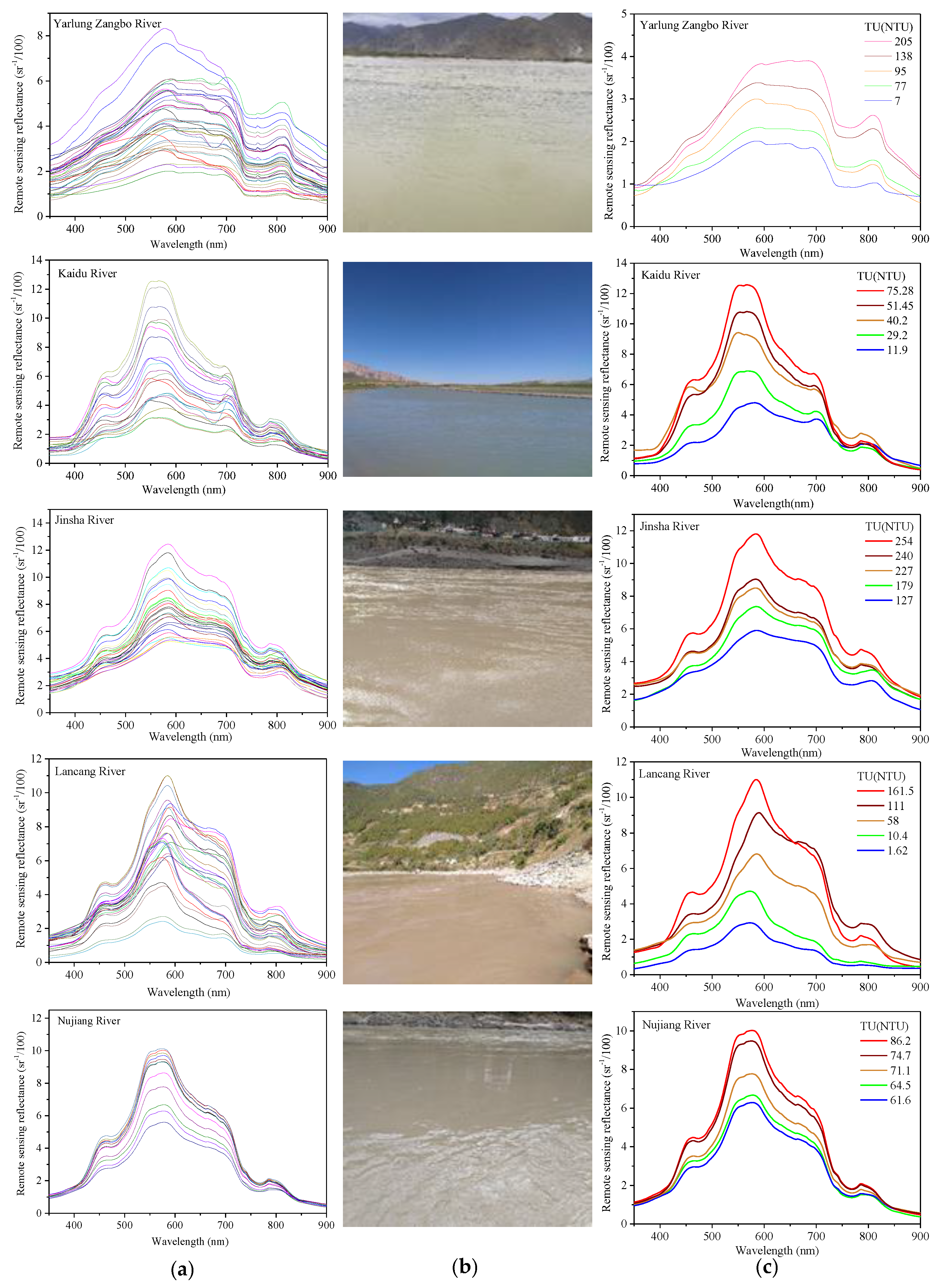
3.2. Spectral Reflectance Properties

The spectra curves of the five rivers were obviously different in shape from those of the ocean water bodies [10,50], but they were similar to the those of inland waters, as shown in Figure 4 [32,40,51,52,53]. In general, the $R_{rs}\left(\lambda \right)$ in the visible band was higher than in the NIR band. In the blue band, the $R_{rs}\left(\lambda \right)$ was very low because of the combined absorption by all optically active constituents, like phytoplankton and CDOM. The $R_{rs}\left(\lambda \right)$ increased in the green band and reached a maximum between 550–580 nm, where the absorption by phytoplankton was minimal and CDOM and TSM mainly affected backscattering. Nonetheless, the reflection peak at the green band was not distinct in YZR, except for a few samples. The $R_{rs}\left(\lambda \right)$ gradually decreased and several characteristics existed in the red band. The second reflection peak presented at around 700 nm. The cause for the peak varied and it mainly depended on the optical characteristics of constituents in water. In the water bodies that were dominated by phytoplankton and its degradation products, the reflection peak was the result of fluorescence induced by phytoplankton photosynthesis. In the water bodies dominated by suspended sediment, the peak was mainly caused by high backscattering of NAP [54,55]. At approximately 675 nm in the red band, some reflection spectra corresponding to KDR samples with high Chl-a concentration had a tough reflection, because the absorption coefficient of Chl-a reached the maximum in the narrow band. The depth of reflection tough was often used to manifest the concentration of Chl-a [40,56]. The absence of the absorption characteristic at 675 nm in all the remaining spectra indicated a lower Chl-a concentration in the study waters, which was consistent with the laboratory analysis results. When the wavelength was longer than 700 nm, the $R_{rs}\left(\lambda \right)$ spectra were less than 0.04sr⁻¹, overall because of the stronger absorption of water molecules in the long-wavelength bands. However, there was a feeble peak at approximately 800 nm that usually resulted from the backscattering of suspended sediment particles.

The magnitude and shape of $R_{rs}\left(\lambda \right)$ exhibited large variability in the five datasets, which indicated that they represent water bodies with different optical properties, from lowly turbid water (e.g., KDR) to highly turbid water (e.g., JSR). Figure 4c shows typical spectra curves corresponding to different turbidity levels of each river. The response of $R_{rs}\left(\lambda \right)$ to increasing turbidity at the five datasets was wavelength-dependent and the two variables showed a positive correlation. Nevertheless, the same $R_{rs}\left(\lambda \right)$ values cannot simply reflect equal turbidity in different rivers. For example, in YZR, the $R_{rs}\left(\lambda \right)$ values corresponding to 77 NTU did not exceed 0.025sr⁻¹, while it was much higher than 0.025sr⁻¹ in KDR and NJR at the nearly equal turbidity levels of 75.28 and 74.7 NTU, respectively. This shows that the relationship between $R_{rs}\left(\lambda \right)$ and turbidity is not a simple linear positive correlation, and the former obviously depends on the unique optical properties of river water bodies. We found that the main suspended particles in KDR came from decayed aquatic grasses and livestock animal excrement, based on field investigation. In YZR, the suspended particles came from soil erosion and pollution discharge of human production and living. In TPR, the suspended particles are sediment caused by fluvial abrasion, soil erosion, and garbage discharge from domestic and construction sources.

3.3. Model Calibration and Validation Using in Situ Data

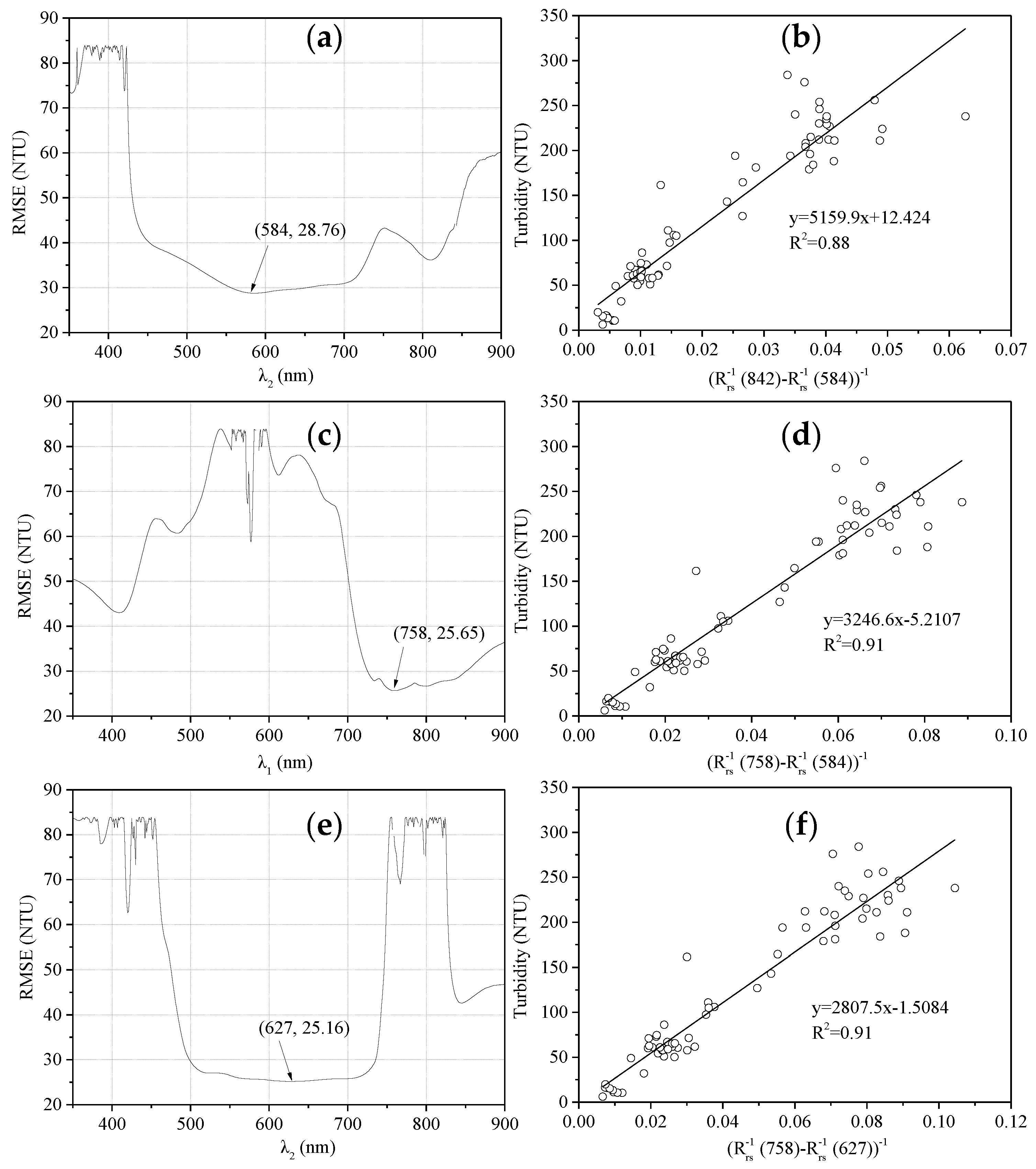
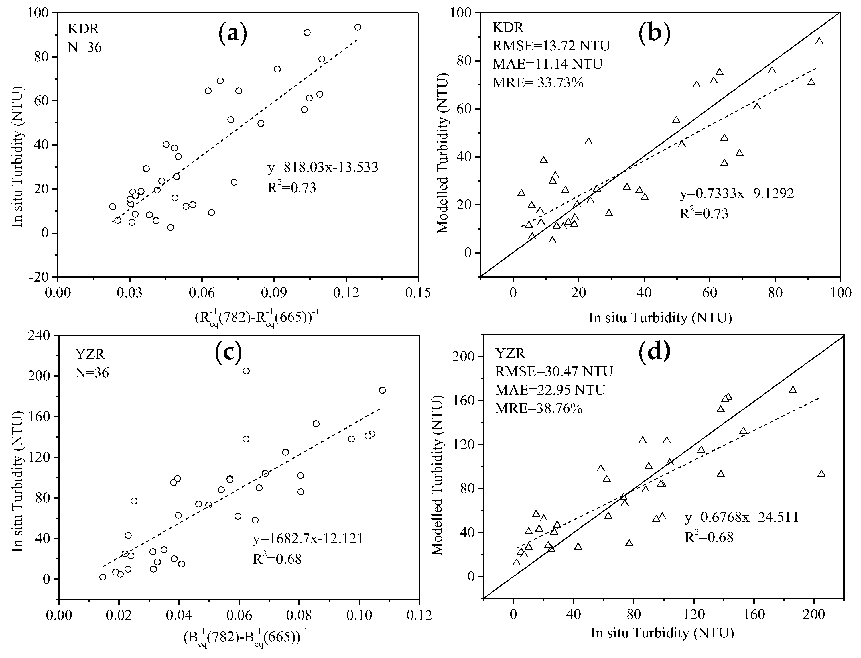
3.3.1. 2BSAT Model Calibration

The 2BSAT model was calibrated using the field data obtained from TPR and validated while using the field data that were obtained from KDR and YZR. The optimal position of the two bands used by the model was determined via stepwise ergodic bands to focus on the minimum RMSE between the measured values and estimated values. We extended the available band range from 350 to 900 nm during the stepwise traversal operation in order to verify the possibility that the optimal position of ${\lambda }_1$ and ${\lambda }_2$ fell in the visible light band range. For instance, we firstly set the initial position of ${\lambda }_1=842$ nm, corresponding to the NIR band of the sentinel-2A, and linearly regressed measured turbidity values versus $R_{rs}{}^{-1}\left(842\right)-R_{rs}{}^{-1}\left({\lambda }_2\right)$ at each single band in the range 350–900 nm. Afterwards, the RMSE of the estimated turbidity values was figured out for locating the optimal position of ${\lambda }_2$, which corresponded to the minimum RMSE. The position of ${\lambda }_2$ was confirmed at 584 nm after the first loop computation (Figure 5a). Once ${\lambda }_2=584$ nm was selected, the same process above was performed to regress $R_{rs}{}^{-1}\left({\lambda }_1\right)-R_{rs}{}^{-1}\left(584\right)$ versus the measured turbidity values for each band in the range 350–900 nm. The RMSE for the second loop computation arrived at a minimum value at 758 nm (Figure 5c). Subsequently, we reset ${\lambda }_1=758$ nm and regressed $R_{rs}{}^{-1}\left(758\right)-R_{rs}{}^{-1}\left({\lambda }_2\right)$ versus the measured turbidity values in the same range. The minimal RMSE was found at 627 nm (Figure 5e). Similarly, the second ${\lambda }_2$ was set at 627 nm to determine the optimal band of ${\lambda }_1$ by assessing the minimum RMSE, and the results showed that the third ${\lambda }_1$ was still 758 nm. Consequently, the 2BSAT model had the optimal accuracy in the case of ${\lambda }_1=758$ nm and ${\lambda }_2=627$ nm. Each round stepwise calculation above reduced the minimum RMSE and increased the fitting degree of $R_{rs}{}^{-1}\left({\lambda }_1\right)-R_{rs}{}^{-1}\left({\lambda }_2\right)$ and the in situ turbidity (Figure 5b,d,f). Finally, the optimal bands of the 2BSAT model were determined based on the 70 field samples that were collected from TPR (Figure 5f). As can be seen from Figure 6, the fitted line (dashed line) of measured and predicted TU values was very close to the 1:1 solid line, and the determination coefficient was 0.91.

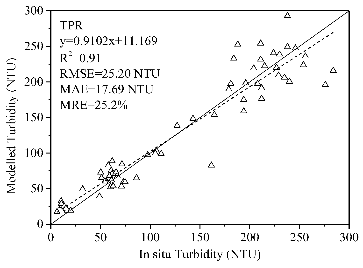
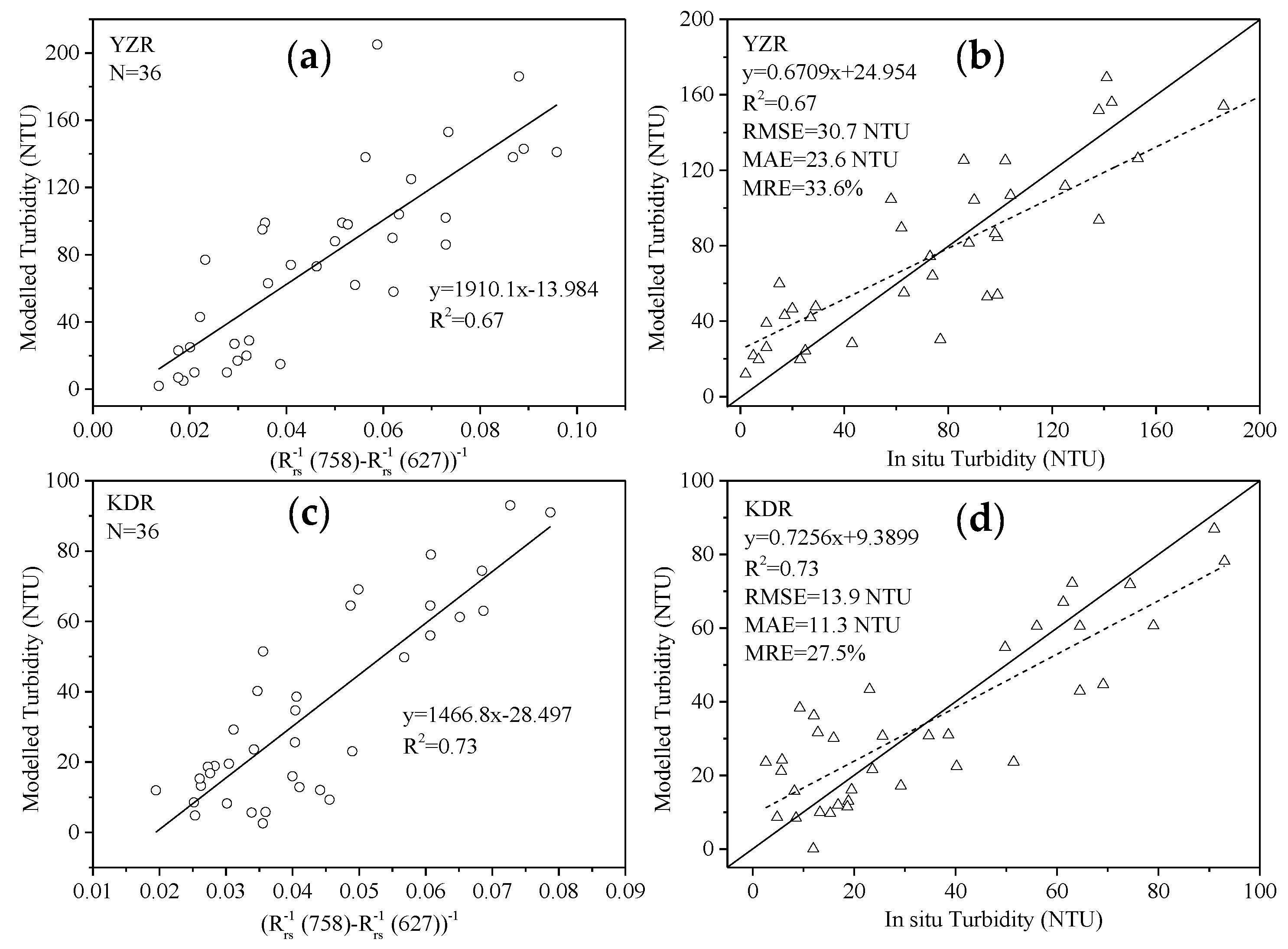
3.3.2. 2BSAT Model Validation

Model validation using an independent observation dataset provides a way to evaluate the reliability of retrieval accuracy and characterize the model uncertainty [21]. We used the water spectra and measured turbidity datasets of YZR (N=36) and KDR (N=36) for model validation in order to accurately evaluate the retrieval accuracy of the 2BSAT model and its applicability to various water bodies in different regions.

Figure 7 shows the comparison between the estimated TU by the 2BSAT model and in situ measured TU in YZR and KDR. The results indicated good agreement between the two values, and the determination coefficients (R²) were 0.67 and 0.73 in the two rivers, respectively. The RMSE, MAE, and MRE were 30.7 NTU, 23.6 NTU, and 33.6% in YZR and 13.9 NTU, 11.3 NTU, and 27.5% in KDR, respectively. Although 2BSAT was only calibrated using TPR data, it could still explain 67% and 73% of turbidity variability for YZR and KDR, respectively, which demonstrates that the 2BSAT model was reliable and stable. Therefore, 2BSAT is an effective approach for deriving TU from hyperspectral data in inland alpine river waters.

It should be noted that the retrieval accuracy in KDR was slightly higher than that in YZR, which could be due to the spectra of KDR being more like the spectra of TPR in terms of curve shape. In addition, MRE in KDR and YZR were both lower than the MRE of 25.2% in TPR. It is not surprising that the development of 2BSAT using only using one geographical region might limit its spatial transportability.

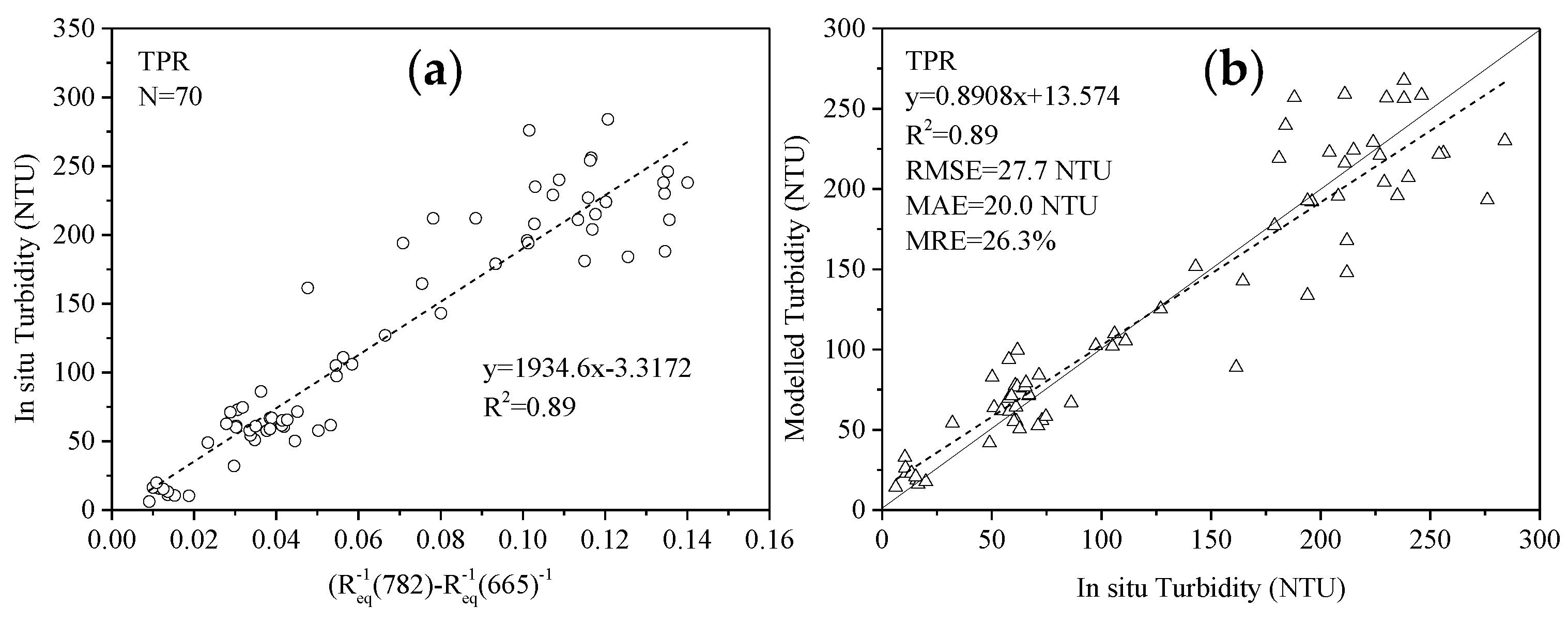
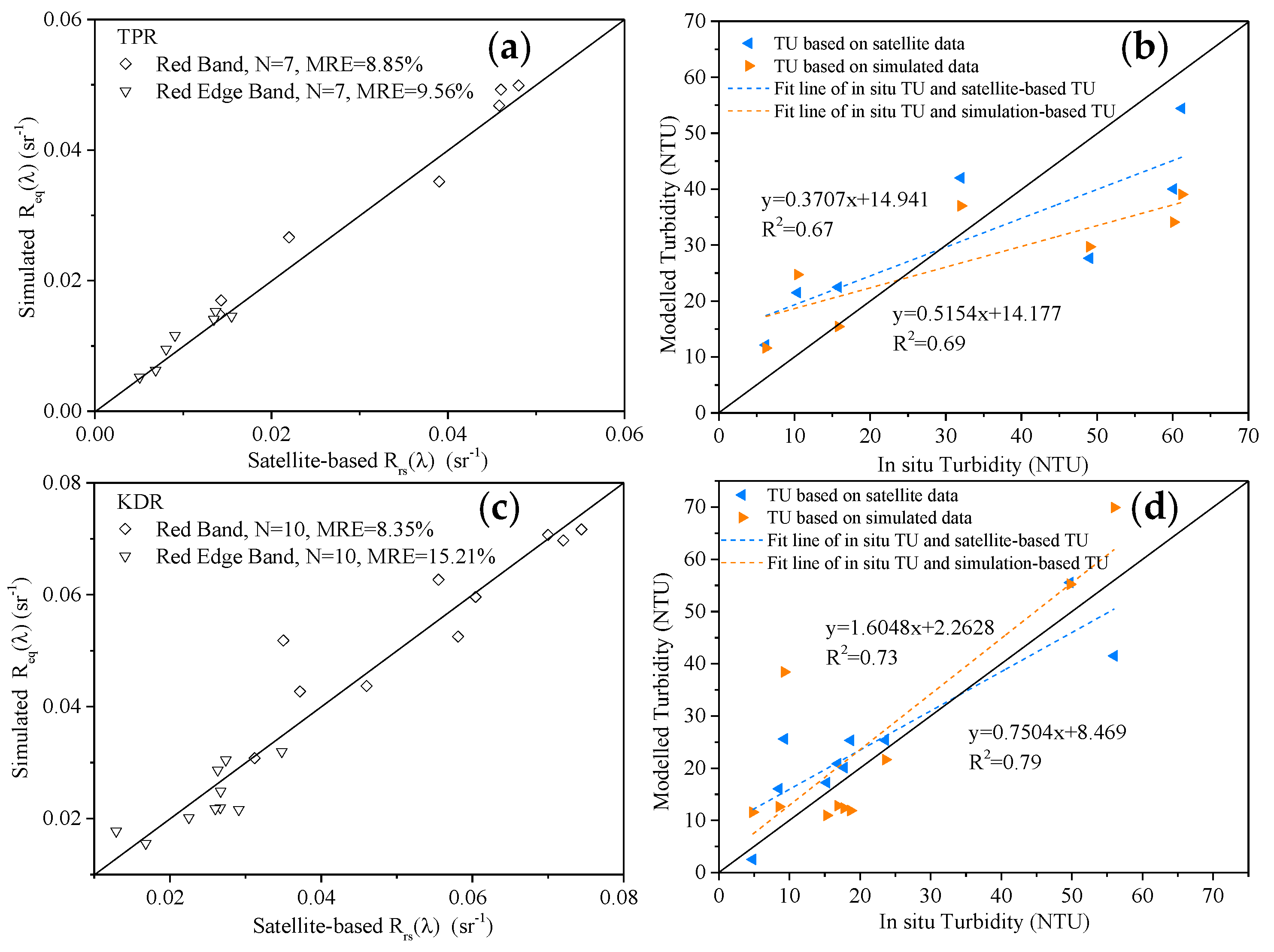
3.4. Model Calibration and Validation Using Simulated Sentinel-2 Bands

The above calibration and validation of the 2BSAT model used a field-measured hyperspectral dataset with 1 nm wavelength increments. However, most of the current Earth observation satellite sensors only have limited multi-spectral bands whose spectral resolution is far wider than 1 nm. In addition, the optimal bands that are determined by in situ hyperspectral optimization (e.g., 758 nm) are not available from the Sentinel-2 MSI sensor. Even some bands may not be available for satellite sensors, because they are not in the atmospheric transmission window [10]. Therefore, it is desirable to tune models spectrally targeted to the Sentinel-2 MSI. Detailed calculations can be found in Section 2.2.3. The adjusted model replaced 758 nm with the MSI red edge band and 627 nm with red band in order to evaluate the 2BSAT performance with Sentinel-2A bands. The central wavelengths at the two bands are 782 nm and 665nm, respectively. Figure 8 shows a strong positive correlation between ${\left(R_{eq}^{-1}\left(782\right)-R_{eq}^{-1}\left(665\right)\right)}^{-1}$ and in situ TU of TPR (R² = 0.89), with RMSE = 27.7 NTU, MAE = 20.0 NTU, and MRE = 26.3% in the modelled TU.

Two independent simulated multispectral band datasets from in situ $R_{rs}\left(\lambda \right)$ data of KDR and YZR were used to verify the model’s predictive ability and transferability in other geographic regions. The accuracy of the model degraded a little in KDR and YZR when compared with the relationship between ${\left(R_{eq}^{-1}\left(782\right)-R_{eq}^{-1}\left(665\right)\right)}^{-1}$ and in situ turbidity from TPR (Figure 9), but a significant correlation still existed between ${\left(R_{eq}^{-1}\left(782\right)-R_{eq}^{-1}\left(665\right)\right)}^{-1}$ and in situ TU, with R² = 0.73 and 0.68, respectively. The result suggests that the 2BSAT has the potential to derive TU while using Sentinel-2 in alpine river waters.

3.5. Turbidity Retrieval

3.5.1. Satellite-based $R_{rs}\left(\lambda \right)$ Versus Simulated $R_{eq}\left(\lambda \right)$

The above calibration and validation of 2BSAT were based on in situ hyperspectral $R_{rs}\left(\lambda \right)$ and simulated equivalent multispectral bands $R_{eq}\left(\lambda \right)$ that corresponded to Sentinel-2 MSI. However, the consistency of satellite reflectance and simulated reflectance needs to be further addressed before applying the 2BSAT model to retrieve the turbidity from river water. This is because the different observational geometries and environments between the field experiment and the satellite may result in different remote sensing reflectance of the same water bodies, even if they both have been atmospherically corrected. Matching data between satellite and in situ data were generated by extracting the pixel values of the satellite images based on the sample position in order to evaluate the reliability of 2BSAT with real satellite data. In some studies regarding ocean color remote sensing, the time interval window between the satellite overpass and field measurement on the same sample site should ideally be within ±3 h [16,57]. However, the time interval window can be extended to ±3 days in lake waters under stable hydrologic and atmospheric conditions [17]. In this study, it is reasonable to choose satellite images with the same date of sampling to match measured data when considering the local climate and hydrological characteristics of the study area and the available overpass satellites. Although we conducted three field campaigns, only two clear Sentinel-2 images in KDR on 21 July 2018 and in TPR on 9 November 2018 were in line with the sampling time. Seven and 10 matchup sites were finalized on the two rivers, respectively. We used a 3×3 pixel box centered on each sample site to extract satellite-based $R_{rs}\left(\lambda \right)$ because of the relatively narrow width of the river. After removing extreme outliers and mixed pixels, the average $R_{rs}\left(\lambda \right)$ value of the remaining pixels was regarded as the effective satellite-based $R_{rs}\left(\lambda \right)$ of the sample site. Figure 10a,c show a comparison of satellite-based $R_{rs}\left(\lambda \right)$ and simulated $R_{eq}\left(\lambda \right)$. The results indicated that the MRE of the remote sensing reflectance at the red band between the two datasets was 8.85% in TPR and 8.35% in KDR, and the MRE at the red edge band was 9.56% in TPR and 15.21% in KDR. Figure 10b,d show a comparison of in situ TU and modelled TU that was based on satellite $R_{rs}\left(\lambda \right)$ and simulated $R_{eq}\left(\lambda \right)$, respectively, which indicated that the determination coefficients (R²) were about 0.7, and a good consistency existed between the two datasets. The above results indicate that satellite-based $R_{rs}\left(\lambda \right)$ and simulated $R_{eq}\left(\lambda \right)$ can both be used to accurately derive TU in TPR and KDR.

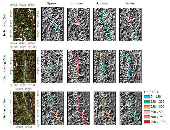
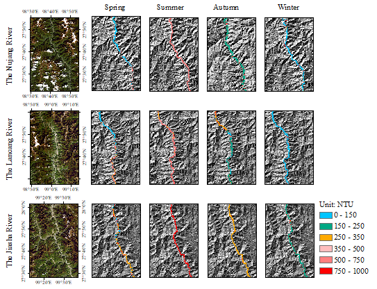
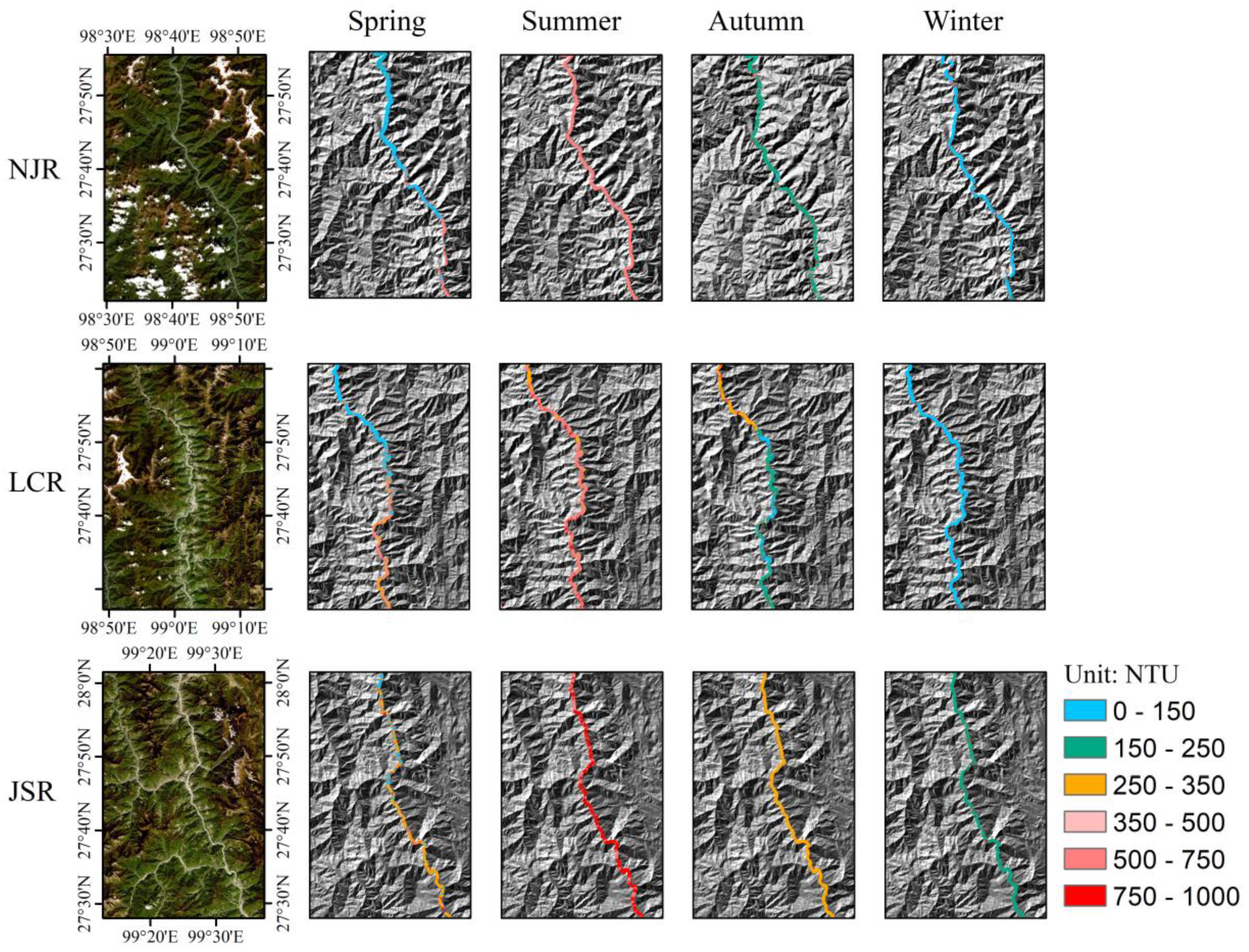
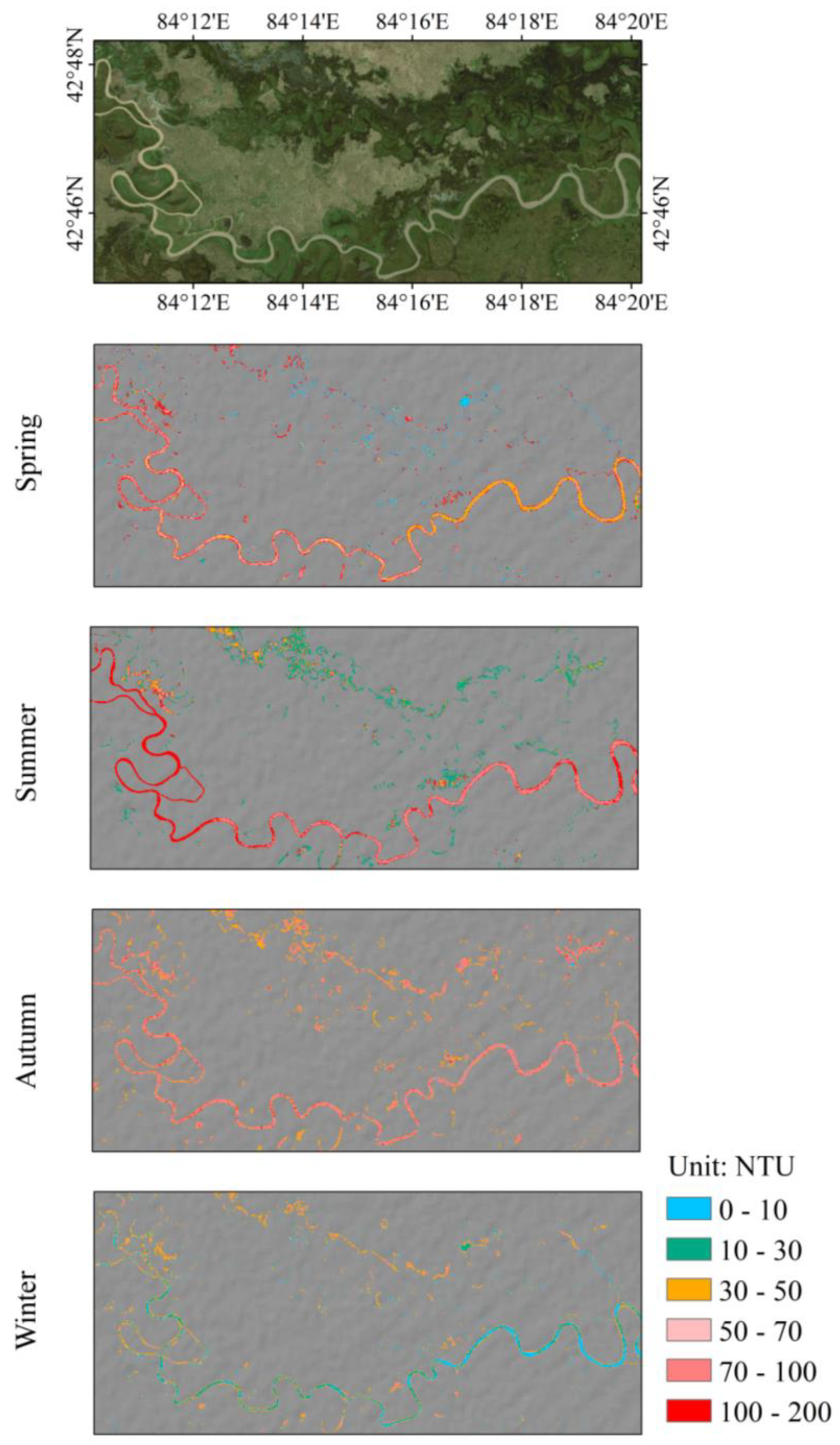
3.5.2. Turbidity Mapping Using Sentinel-2 Images

It can be determined that the 2BSAT model has excellent performance in retrieving TU in alpine rivers based on the above comprehensive analysis. Therefore, this study applied the model to map the temporal–spatial distribution of turbidity and analyzed the seasonal turbidity patterns in TPR, KDR, and YZR, respectively. The season division was defined by month, as follows: spring included March, April, and May; summer included June, July, and August; autumn included September, October, and November; and, winter included December of the current year and January and February of the following year. The average of retrieval turbidity from all the images during each season represents the turbidity level of the season. Thus, all available Sentinel–2 images with no or few clouds from the autumn of 2018 to the summer of 2019 were processed to recognize the seasonal turbidity patterns of the five rivers.

Figure 11 shows the spatial distribution and seasonal variation of turbidity in the NJR, LCR, and JSR in the same latitude interval of the TPR area. It was observed that the turbidity of the three rivers was quite varied in different seasons, but they all had one thing in common: the three rivers presented the highest turbidity in summer, followed by spring and autumn, and the lowest in winter. The average turbidity for each season in the three rivers is shown in

Table 5. The average turbidity (unit: NTU) for each season in the Nujiang River (NJR), Lancang River (LCR), and Jinsha River (JSR).

	Spring	Summer	Autumn	Winter
NJR	124.8	548.7	196.3	83.5
LCR	234.1	524.8	174.4	56.7
JSR	265.2	779.5	292.3	182.4

. The results also indicate that the average turbidity in all seasons in JSR was higher than that in NJR and LCR. In addition, the average turbidity in autumn in NJR and JSR was higher than in spring, but the situation was just the opposite in LCR. It should be noted that such seasonal turbidity differences also have different performances in different reaches of the same river, like in LCR.

Figure 12 shows the spatial distribution of turbidity in each season in KDR. Similar to the TPR, the turbidity of the river was the highest in summer and the lowest in winter. However, the difference was that the turbidity of lakes presented the highest in autumn. We also note that the amount of water in the Bayanbulak Wetland significantly increased during the summer, and the number and area of small lakes and ponds increased simultaneously. At the same time, it is obvious that the turbidity of calm lake waters in summer was lower than that of the dynamically flowing river mainstream waters. In addition, the decreasing velocity of turbidity of lake waters from autumn to winter was not as fast as that of rivers, because the turbidity of lake waters in winter was significantly higher than that of rivers. The different hydrodynamic conditions between rivers and lakes may account for the seasonal turbidity differences. The quantitative calculation results showed that the average turbidity in each season in KDR was as follows: 42.6 NTU in spring, 106.7 NTU in summer, 37.5 NTU in autumn, and 12.3 NTU in winter.

Figure 13 shows the spatial distribution and seasonal variation of turbidity in the intersection reach of the YZR and the Lhasa River. The turbidity of the mainstream of YZR reached its maximum in the summer, similar to the other two basins, which corresponds to the wet season of this basin. However, the turbidity in the Lhasa River reached its maximum in the autumn. The range of turbidity variations in Lhasa River was relatively small when compared with the large amplitude of turbidity variation of the YZR mainstream between seasons. We also noticed that the influx of the tributary led to a decrease in the turbidity of the water body on the north side of the YZR mainstream during the summer. The average turbidity of YZR was as follows: 16.4 NTU in spring, 160.6 NTU in summer, 61.9 NTU in autumn, and 22.3 NTU in winter. The average turbidity of the Lhasa River inlet was as follows: 11.5 NTU in spring, 13.2 NTU in summer, 54.1 NTU in autumn, and 8.6 NTU in winter.

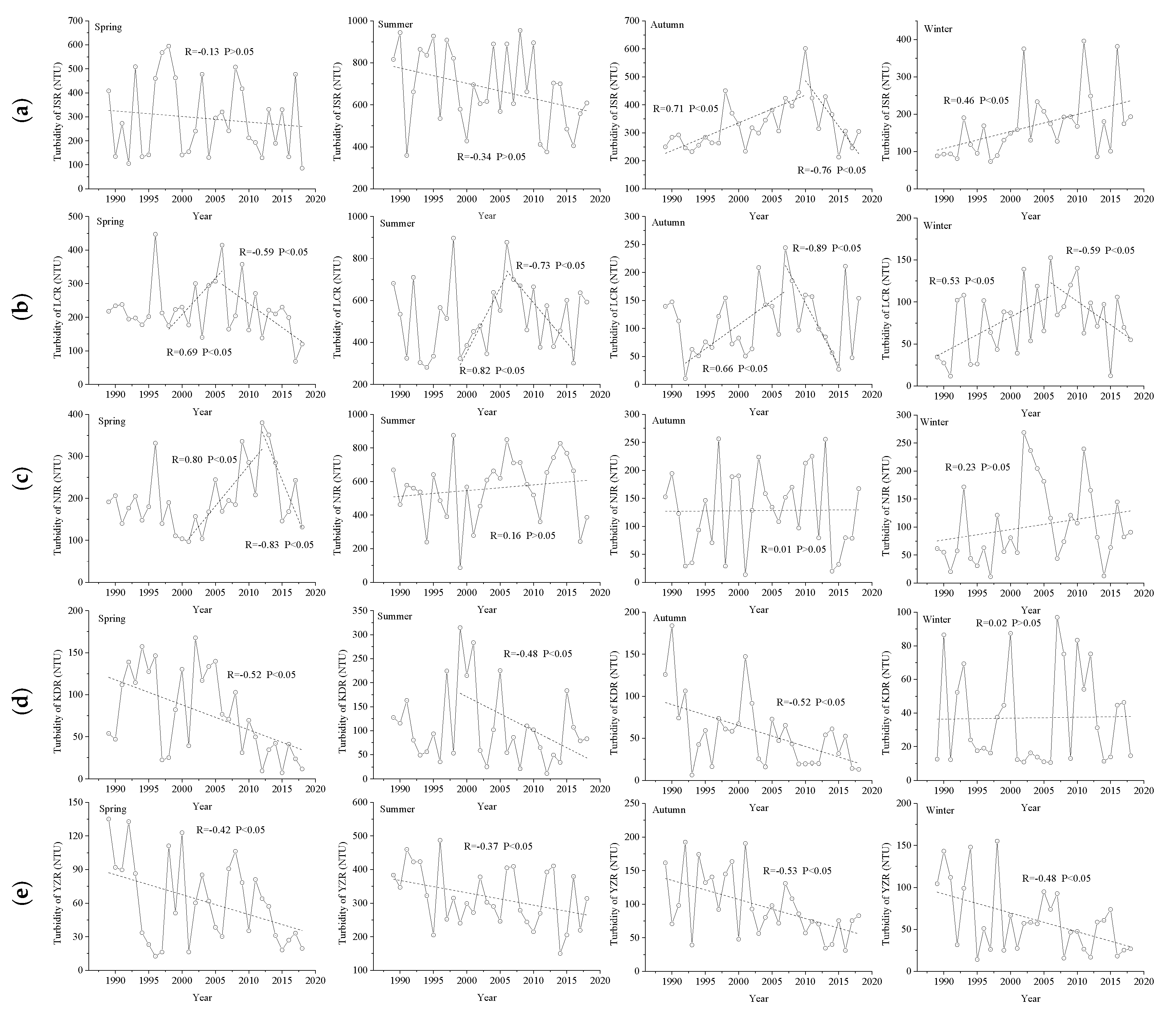
3.5.3. Long-term Seasonal Turbidity Change from 1989 to 2018

From the analysis in Section 3.5.2, it was observed that obvious seasonal variation characterized the turbidity of river waters. We used the Landsat series images from 1989 to 2018 to derive turbidity in the five rivers for further analysis of the long-term seasonal characteristics and variation tendency of river turbidity. Not only can Landsat series images provide long-term series data, but the data also have a good consistency with the Sentinel-2 product [17,58]. We adopted the red band and the NIR band that were closest to the bands adopted from Sentinel-2 MSI to build the 2BSAT model since the Landsat series images have few bands. The calibration procedure of the 2BSAT model parameters while using the Landsat data was the same with the Sentinel-2 data.

Figure 14 shows the long-term seasonal change of turbidity in the five inland rivers over the past 30 years. The dashed lines in the graphics represent the variation tendency of turbidity. The statistical results showed that the variation ranges of turbidity in the TPR were higher than that of KDR and YZR (

Table 6. The seasonal average turbidity (unit: NTU) in the five rivers from 1989 to 2018.

	Spring	Summer	Autumn	Winter
JSR	293.3	677.2	329.3	169.7
LCR	224.3	520.6	110.5	76.7
NJR	199.2	558.0	128.1	102.1
KDR	77.5	106.9	56.3	37.1
YZR	61.3	317.9	97.1	61.8

and Figure 14). It can be determined that the turbidity of the five rivers usually reached a maximum in summer, while reaching a minimum in winter, which is consistent with the results presented in Table 5. In addition, the 30-year variation tendency of turbidity in the five rivers differed from one another. In the JSR, the turbidity in autumn showed an uptrend before 2010 and then decreased, but, overall, it showed an uptrend in winter. In the LCJ, 2006 seems to be a time sub-node of turbidity trend change. For a long time before 2006, the turbidity showed an increase in spring, summer, and winter, and it then it decreased. In the autumn, the time node was postponed to 2007. In the NJR, the turbidity gradually increased in spring from 2001 to 2013, and it then decreased. However, there was no significant change trend in other seasons. In the KDR, Turbidity showed a downward trend in spring, summer (after 1999), and autumn. In the YZR, the downward trend of turbidity was present in all four seasons, and the trend was more obvious than other rivers, overall, over the past 30 years.

It is easy to see that the variations of river turbidity in the TPR basin do not have obvious regularity by comparing the seasonal changes of turbidity in the long-term series of five rivers. The possible explanation is that natural disasters, such as landslides and mudslides in the area, had a sudden impact on seasonal average turbidity. While the geological conditions of the KDR and YZR are relatively stable, the turbidity changes of the two rivers were smaller and showed a long-term dynamic variation trend.

4. Discussion

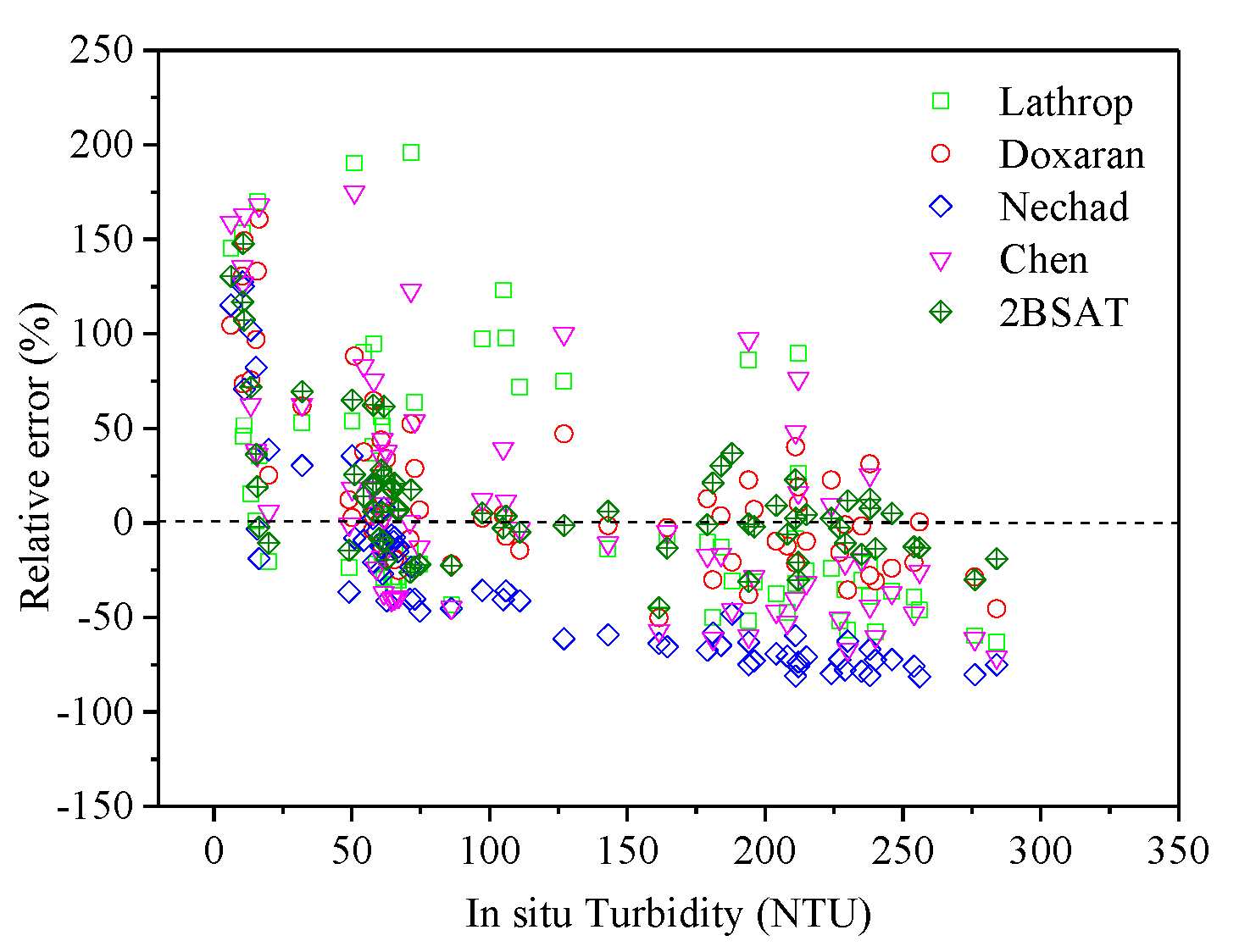
4.1. Performance of the Four Existing Turbidity Models

In existing research on water quality monitoring, the diversity of water optical properties in different regions often requires an adjustment of model parameters to improve its regional adaptability. Therefore, the specific parameters of the four existing models—Lathrop, Chen, Nechad, and Doxaren (

Table 7. Four existing TU quantitative retrieval models.

Model	Simplified Description
Chen [16,29]	${{\displaystyle r}}_{rs}(\lambda )=\frac{{{\displaystyle R}}_{rs}(\lambda )}{0.52+1.7{{\displaystyle R}}_{rs}(\lambda )}$
	$s(\lambda )=\frac{b_{bt}(\lambda )}{a_t(\lambda )}=\frac{-{{\displaystyle g}}_0+{[{({{\displaystyle g}}_0)}^2+4g_1{{\displaystyle r}}_{rs}(\lambda )]}^{0.5}}{2g_1+g_0-{[{({{\displaystyle g}}_0)}^2+4g_1{{\displaystyle r}}_{rs}(\lambda )]}^{0.5}}$, ${{\displaystyle g}}_0=0.0364,{{\displaystyle g}}_1=0.348$
	${{\displaystyle b}}_b(660)\propto \frac{s(660)}{s(560)-\epsilon \ast s(485)}$, $\epsilon =0.7155$
	$\mathrm{TU}=159.21\ast \ln ({{\displaystyle b}}_b(660))+67.07$
Nechad [12,15]	${{\displaystyle a}}_t(\lambda )={{\displaystyle a}}_p(\lambda )+{{\displaystyle a}}_{np}(\lambda )$, ${{\displaystyle b}}_{bt}(\lambda )={{\displaystyle b}}_{b,p}(\lambda )+{{\displaystyle b}}_{b,np}(\lambda )$
	${{\displaystyle a}}_{pT}(\lambda )=\frac{{{\displaystyle a}}_p(\lambda )}{\mathrm{TU}}$, ${{\displaystyle b}}_{pT}(\lambda )=\frac{{{\displaystyle b}}_{b,p}(\lambda )}{\mathrm{TU}}$
	$C=\gamma \frac{{{\displaystyle b}}_{pT}(\lambda )}{{{\displaystyle a}}_{pT}(\lambda )+{{\displaystyle b}}_{pT}(\lambda )}$, $A=\frac{{{\displaystyle a}}_{np}(\lambda )}{\gamma {{\displaystyle b}}_{pT}(\lambda )}$
	$\mathrm{TU}=\frac{A\ast {{\displaystyle R}}_{rs}(681)}{1-{{\displaystyle R}}_{rs}(681)/C}+B$, $A=931.61,B=0.11,C=1.53$
Lathrop [59]	$\mathrm{TU}=a\ast \exp (b\frac{{{\displaystyle R}}_{rs}(660)}{{{\displaystyle R}}_{rs}(560)})$, $a=1.775,b=5.4676$
Doxaran [60]	$\mathrm{TU}=a(\frac{{{\displaystyle R}}_{rs}(850)}{{{\displaystyle R}}_{rs}(550)})+b$, $a=559.98,b=0.9117$

)—were tuned according to the bio-optical information that was sampled from the five rivers in this study.

The Chen model is a semi-analytical model that uses a combination of three bands in the visible range to estimate the backscattering coefficients at 660 nm of the water bodies. Subsequently, the best fit function between TU and $s\left(660\right)/\left(s\left(560\right)-\epsilon \ast s\left(485\right)\right)$ is calculated based on least-squares regression analysis. The Nechad model that is based on the IOPs of water bodies establishes the quantitative relationship between the water-leaving reflectance and TU by defining turbidity-specific particulate absorption and turbidity-specific backscattering. In this study, we replaced water-leaving reflectance with remote sensing reflectance. The Lathrop and Doxaren model used the band ratio as the variable factor to estimate the turbidity by the exponential and the linear function, respectively. Table 7 shows the optimal formulas of the above four models tuned while using the TPR data. The performance evaluation of the four models was based on the comparison of the predicted TU with in situ TU.

By comparison, it was found that the Doxaren model produced a superior performance to the other three models, and using the model could account for 75% variation in TU in the TPR (Figure 15). However, when the turbidity in waters was <70 NTU, the predicted TU values by the model were significantly higher than the measured TU. It is worth noting that the Nechad model only has practical feasibility in water bodies less than 70 NTU, while the predicted TU is much lower than the measured TU in higher turbidity waters. The predicted TU of the Chen and Lathrop model were too discrete when compared to the measured TU, which resulted in them only accounting for about 30% variation in TU. These findings imply that the Doxaren model is a more viable model for estimating the turbidity of TPR waters when compared to the other three models. However, another study has shown that the Lathrop model produces good performance in deriving the TSM concentration from turbid coastal waters [16]. This might result from the differences in optical properties of coastal waters and inland river waters.

4.2. Turbidity Model Evaluation and Comparison

The relative error results showed that the 2BSAT model (MRE = 25.2%) had superior accuracy performance in comparison to the Lathrop (MRE = 41.3%), Chen (MRE = 43.8%), Nechad (MRE = 50.9%), and Doxaren (MRE = 28.2%) models. Figure 16 shows that the scatter plot of the relative error of the 2BSAT model was more concentrated than the other four models. Moreover, the 2BSAT model accounted for approximately 91% turbidity variation in TPR, which was >50% higher than the Lathrop, Chen, and Nechad models, and 16% higher than the Doxaren model (Figure 6 and Figure 15). In addition, the 2BSAT only needed the red and NIR bands to build the relationship between TU and water optical properties in turbid rivers. These results imply that the 2BSTA model is more efficient than the above four models and it can be used to accurately estimate TU in alpine rivers.

The main principle of the Chen model is based on the assumption that the absorption and the backscattering coefficient of water between two neighboring wavelengths vary linearly [29]. The linear slope of backscattering depends on all particulate matter, and the linear slope of absorption depends on phytoplankton, suspended particles, and CDOM in waters. Based on the assumption, the backscattering coefficient can be isolated from remote sensing reflectance. Moreover, local bio-optical characteristics of river estuaries and coastal waters determine the slope coefficients [29]. This is to say that these parameters are generally appropriate for waters with similar optical properties as these types of water. However, the optical properties of inland water bodies are significantly different from those of coastal water. We used the original parameters of the Chen model to estimate the backscattering coefficient at 660 nm, which was further used to estimate turbidity by least-squares regression, because of the lack of measured values of the absorption and backscattering coefficients of various substances in the five rivers in this study. It is not surprising that the accuracy of the Chen model was not very satisfactory (Figure 15b). Therefore, it is necessary to re-optimize the model parameters according to the optical properties of the specific water bodies for guaranteeing the retrieval accuracy, but this undoubtedly limits the universality of the model.

The Nechad model that is based on the IOPs model builds the quantitative relationship between turbidity and water-leaving reflectance [12]. The model assumes that non-particulate backscattering can be negligible when compared to particulate backscattering in highly turbid waters and defines the turbidity-specific particulate absorption $a_{pT}\left(\lambda \right)$ and $b_{pT}\left(\lambda \right)$ turbidity-specific backscattering (Table 7). Without considering the error coefficient B, A and C are the main parameters that need to be calibrated, which are derived from above turbidity-specific bio-optical variables. In Nechad’s study, C was calibrated while using “Standard” IOP data, and A was calibrated by non-linear regression analysis between in situ hyperspectral reflectance and TU [15]. Based on in situ data obtained from TPR, we re-optimized the parameters applicable to the water quality characteristics of the inland alpine rivers. However, the results (Figure 15c) showed that the Nechad model could only account for 31% variation in deriving turbidity from the TPR. Furthermore, the model significantly underestimated TU when the TU was higher than 70 NTU. This poor accuracy indicated that the reflectance at 681 nm was not applicable to derive turbidity in inland rivers. In addition, the optical effect of pigments and CDOM in water makes an important contribution to the spectrum, which seriously interferes with the extraction of backscattering signals from the single-band reflectance. Therefore, the optical effect of non-particles in the water, especially in optically complex waters, affected the output of the single band model.

The Lathrop model and Doxaran model use a two-band ratio as the independent variable to retrieve water turbidity. The difference is that the former adopts the Red-Green band ratio and the latter adopts the NIR-Green band ratio. The Lathrop model adopts an exponential function while the Doxaran model adopts a linear function for typifying the turbidity best because of the difference in sensitivity of different bands to turbidity (Table 7). The Lathrop model might produce poor performance in the turbid productive waters since it relies strongly on remote sensing reflectance in the green and red bands. This is because Chl-a has a significant effect on the shape and magnitude of spectra in the band range. Thus, the Doxaran model replaced the red band in the Lathrop model with a NIR band for reducing the effect of absorption from Chl-a. The performance of the Doxaran model was better than the Lathrop model when comparing the predicted turbidity with the measured turbidity (Figure 15a,d). The determination coefficient of the former was 0.75, which was 127% higher than the latter. However, the strong absorption of water molecules in the NIR region reduced the signal-to-noise ratio and enhanced the interference of inherent noise [61]. Such inherent noise cannot be eliminated by the band ratio and then still affect the output of the model.

Fortunately, the 2BSAT Model could minimize the above negative effects in the Lathrop, Chen, Nechad, and Doxaran models. The model used the difference of the reciprocal of remote sensing reflectance at two neighboring bands to isolate the backscattering. Using the division factor is beneficial in reducing the effect of non-particles and measurement errors on remote sensing reflectance. The results indicated that the 2BSAT model worked better than the other four models in TPR (Figure 16). However, some aspects of the model still need further improvement. Firstly, turbidity is an optical parameter. Not only does the TSM concentration affect the turbidity of the water, but the physical properties of the particles, such as size distribution, shape, and surface roughness, also affect it [62]. This means that the turbidity of water bodies with the same concentration of TSM might not be the same. Moreover, turbidity in the five rivers presents significant seasonal characteristics in different seasons (Figure 11, Figure 12 and Figure 13). Nevertheless, the in situ data that were used in this study were only obtained from the single–field observation campaign for each river and lacked sequenced measurements over a long time. These data are insufficient in validating the accuracy of the 2BSAT model in different seasons that have different bio-optical properties. Therefore, it will be beneficial to improve the model’s applicability by using multi-temporal and various bio-optical conditions water data. It is worth noting that the original assumption of the 2BSAT model is valid in the water bodies dominated by suspended particles, ignoring the effects of other components, such as chlorophyll-a. However, when applied to the low Chl-a concentration of water, like the KDR, the 2BSAT model can also guarantee a high accuracy (Figure 7d and Figure 9b). In addition, the specific parameters of the 2BSAT model in TPR, KDR, and YZR are different from each other, because the main causes of turbidity in these basins are dissimilar. This indirectly illustrates the dependence of the 2BSAT model on the optical properties of river water.

4.3. Factors Affecting River Turbidity

In this section, we discussed the influencing factors of river turbidity and briefly analyzed the seasonal patterns of some river reaches. There are too many factors causing the turbidity of river water, including natural factors, such as heavy rainfall, mudslides, and landslides, as well as human factors, such as engineering construction, pollution discharge, and so on. Here, we only selected a few factors according to local characteristics of basins, including cascade hydropower stations, sewage discharge and road construction, and precipitation. The factors affecting turbidity did not act in the same manner over the three study basins, and they may present different levels of importance in each river. The integrated spatial–temporal approach was very useful in understanding the seasonal turbidity patterns of these factors in inland rivers.

4.3.1. Cascade Hydropower Stations

15 hydropower stations were constructed along the mainstream of the river in Yunnan Province because of the abundant waterpower resources and favorable geographical conditions of the LCR. The development of hydropower resources has greatly affected eco-hydrological processes in the upper reaches of the river [63]. We analyzed the spatial distribution of seasonal turbidity in the upstream and downstream of Tuoba, Huangdeng, Dahuaqiao, and Miaowei hydropower stations in order to monitor the effect of hydropower stations on river turbidity (Figure 17). The four hydropower stations are located in the upper reaches of the LCR with an average distance of 56km. They are part of the hydropower base of the Lancang River trunk stream. The cascading development of hydropower has changed the original continuity of rivers, which results in changes in the physical, chemical, and biological factors of river waters [64]. Moreover, changes to hydrodynamics provide the conditions for large amounts of sediment and nutrients to subside in the reservoir, which greatly reduces the sediment concentration in the discharge water. However, Figure 17 shows that the turbidity of the downstream waters of these hydropower stations was usually higher than that of the reservoir waters. This is because the strong physical disturbances that are caused by the discharge of water and faster flow velocity prevent sediment from sedimentation downstream. The seasonal patterns of turbidity in the waters near these hydropower stations agreed with that in other river reaches, which shows that the turbidity was higher in spring and summer and lower in autumn and winter. This indicates that seasonal factors have a greater impact on river turbidity than hydropower stations.

4.3.2. Sewage Discharge and Road Construction

The land use patterns along these rivers have undergone rapid changes with the development of township leisure tourism and modern agriculture and the growth of the population, including deforestation, urban expansion, and shrinking farmland, which result in more pressure on water resource protection. In recent years, township domestic sewage discharge along the river has attracted more and more attention [65]. Centralized collection of rural sewage is relatively difficult because of the low emissions and scattered location. Meanwhile, sewage treatment lacks funds for operation and maintenance of facilities and routine supervision and administration. As a result, township domestic sewage cannot be effectively treated and it has become a major constraint for river environmental improvement. Especially for the densely populated TPR and YZR basin, it is an urgent problem to regulate sewage discharge.

The construction of various projects along the river also has a negative impact on river water quality. Construction activities, such as foundation leveling and road and bridge construction, need to shift large amounts of soil and rock, but this may cause damage to vegetation, geomorphology, and water systems. The excavation surface along the river in road construction usually forms a steep slope that is generally larger than the slope of the original natural surface. Due to its low stability, once external forces, such as rainfall, runoff, wind, mechanical vibration, and so on, stimulate the excavation surface, it often induces collapse and causes a lot of soil erosion. This is also one of the causes of the frequent landslides in the TPR basin.

In this section, we took a small reach upstream of the NJR as an example (Figure 18). In the true color image of Figure 18, on the west bank of the river is a small town, and on the east bank in the red oval mark is a road construction site, which corresponds to the leftmost field photo. The result of the field investigation showed that a large amount of domestic garbage from the town and sewage from cultivation farms close to the river were directly discharged into rivers without any treatment. In addition, road construction also discharged a large amount of soil and stone into the river, which raised the riverbed and reduced the width of the river. The rushing river water hits the raised rock at the bottom of the river, which causes sediment resuspension. Therefore, the discharge and hydrodynamics led to the turbidity of this reach being higher than other reaches. This phenomenon manifested in every season during construction, even in winter at low turbidity levels. However, it is necessary to take measures to eliminate the influence of these factors because of the effects of ripples and whitecaps of river water on image reflectance.

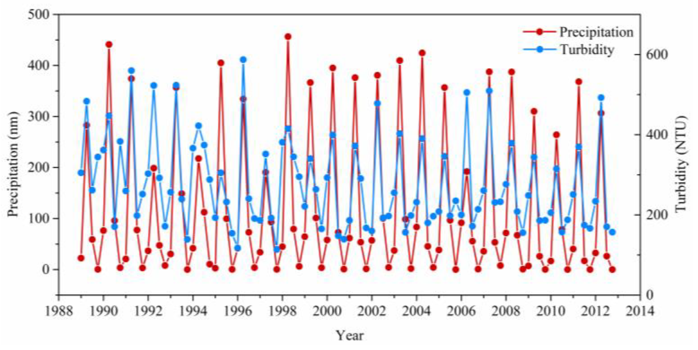
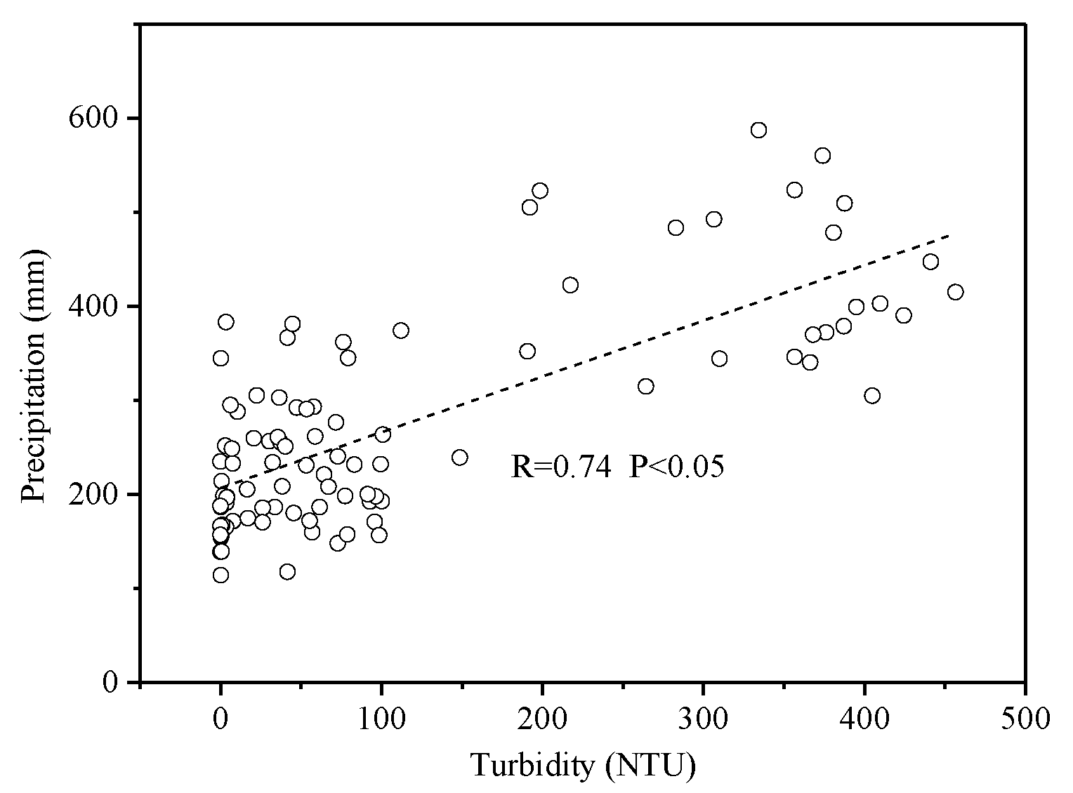
4.3.3. Precipitation

Precipitation causes the soil and pollutants on the underlying surface to drain into the river through runoff, thereby increasing the turbidity of the river. Summer is the rainy season in the five rivers in this study, which is one of the reasons why these rivers usually present the highest turbidity in this season. In addition, heavy rainfall in geologically unstable regions, like the TPR, usually results in landslides and mudslides. The large amount of viscous mud and solid debris flowing into the river will significantly increase the turbidity of the river in a short time. Therefore, precipitation is one of the important factors that affect the turbidity of water bodies. We collected precipitation data from the Lhasa meteorological stations near the Lhasa River inlet reach in the YZR basin and analyzed the relationship between precipitation and river turbidity in order to analyze the impact of precipitation. The precipitation data are the total precipitation in each season from 1989 to 2012, and the turbidity is the average in each season from 1989 to 2012. The results showed that turbidity changed with precipitation and it usually reached the highest level when the precipitation was maximum (Figure 19). Thus, there is a clear correlation between precipitation and river turbidity and the correlation coefficient between the two reaches 0.74 (Figure 20), which indicates that precipitation indeed has an effect on the turbidity of river water.

5. Conclusions

We proposed a reliable 2BSAT model using red and NIR bands to retrieve turbidity in inland alpine rivers based on the characteristics of optical properties of alpine river waters and bio-optical theory. We initially used in situ hyperspectral data to determine the optimal bands by stepwise traversal technology. Afterwards, the simulated multispectral remote sensing reflectance data were calculated and compared with the synchronous satellite-based remote sensing reflectance in order to verify the applicability of the 2BSAT to high spatial resolution Seninel-2 images. The results indicated a good consistency between the two reflectance data (MRE<16%), and the determination coefficient of the 2BSAT model based on the satellite-based remote sensing reflectance was >0.65 in retrieving turbidity from the TPR and KDR. Finally, based on the 2BSAT model, we used the Sentinel-2 images to analyze the spatial distribution and the seasonal patterns of turbidity and Landsat images to analyze the long-term sequenced turbidity variation from 1989 to 2018. The findings of the study are summarized, as follows.

(1)

The 2BSAT model was calibrated and validated while using one calibration dataset from the TPR and two independent validation datasets that were obtained from the KDR and YZR, respectively. The study results indicate that the 2BSAT model is reliable and robust in retrieving turbidity in alpine rivers from clear to highly turbid water bodies. Moreover, there is no need to reselect the bands, even though parameter optimization is required for improving the accuracy of the retrieval results.

(2)

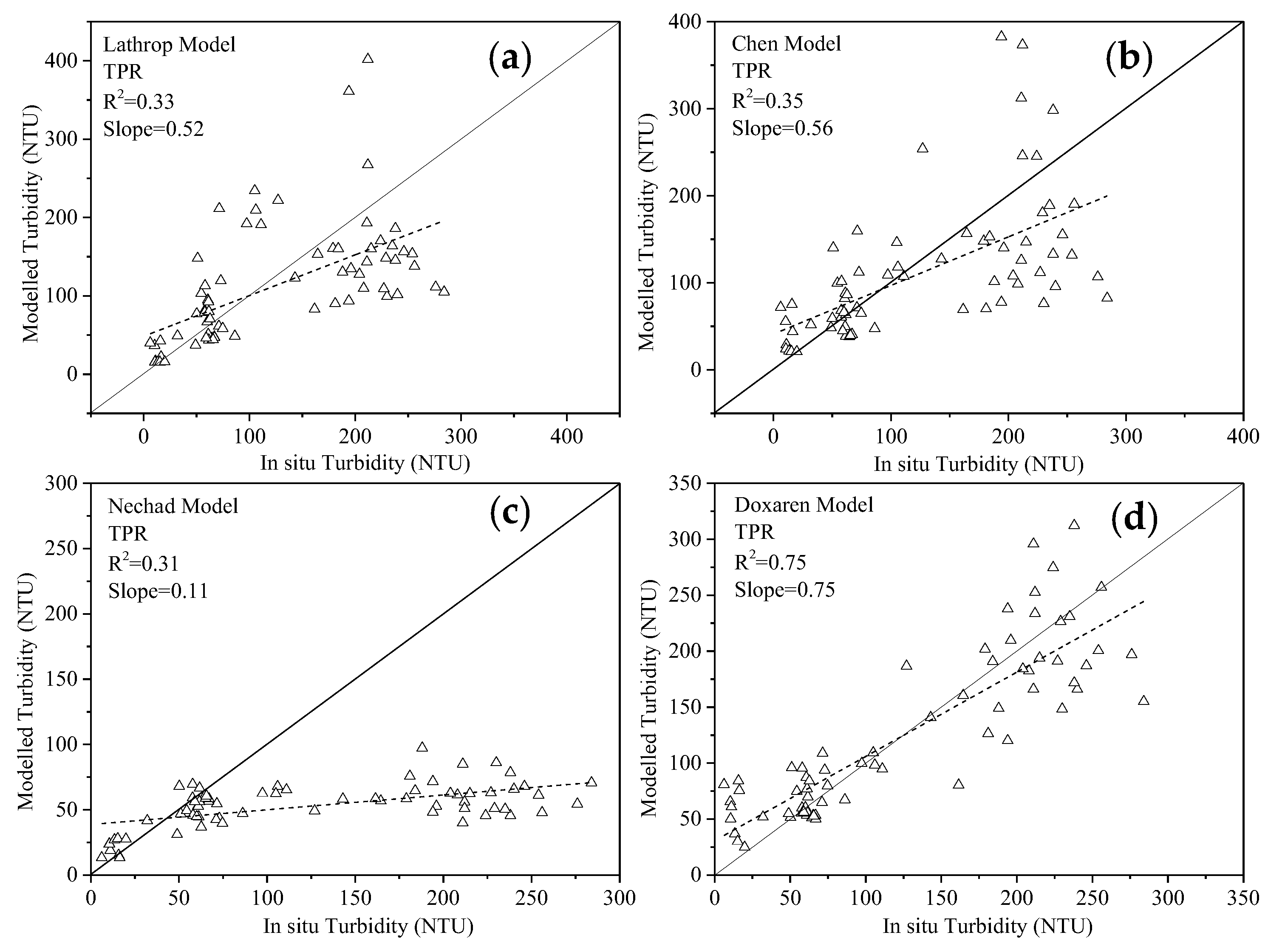
Based on in situ hyperspectral data, the 2BSAT model produced a superior performance in deriving the TU from alpine rivers in comparison to the Lathrop, Chen, Nechad, and Doxaren models. It was confirmed that the 2BSAT model, in estimating the TU, decreased the uncertainty by 36%, 40%, 48%, and 6% of the MRE values, respectively, from the above 4 models in the TPR.

(3)

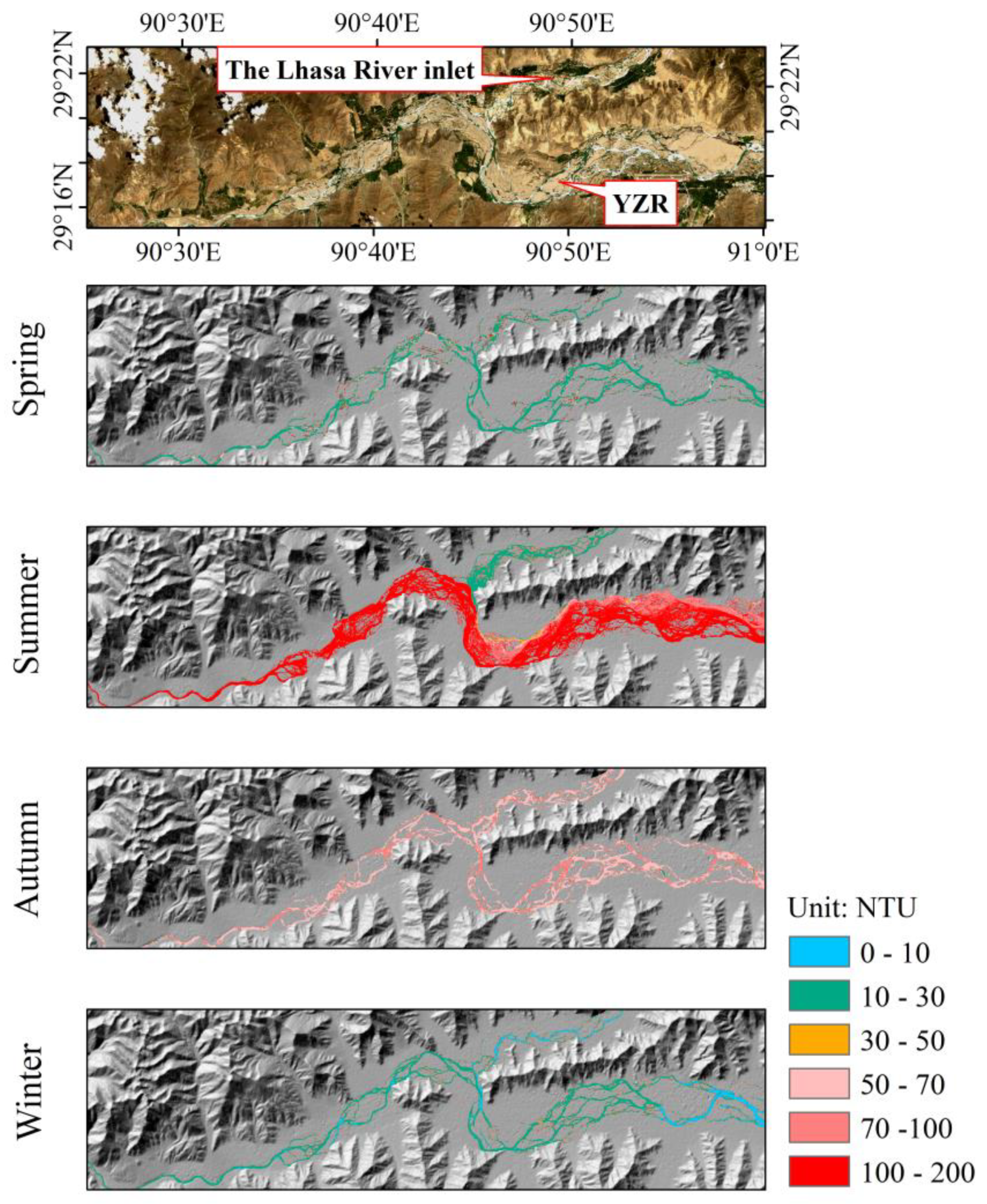
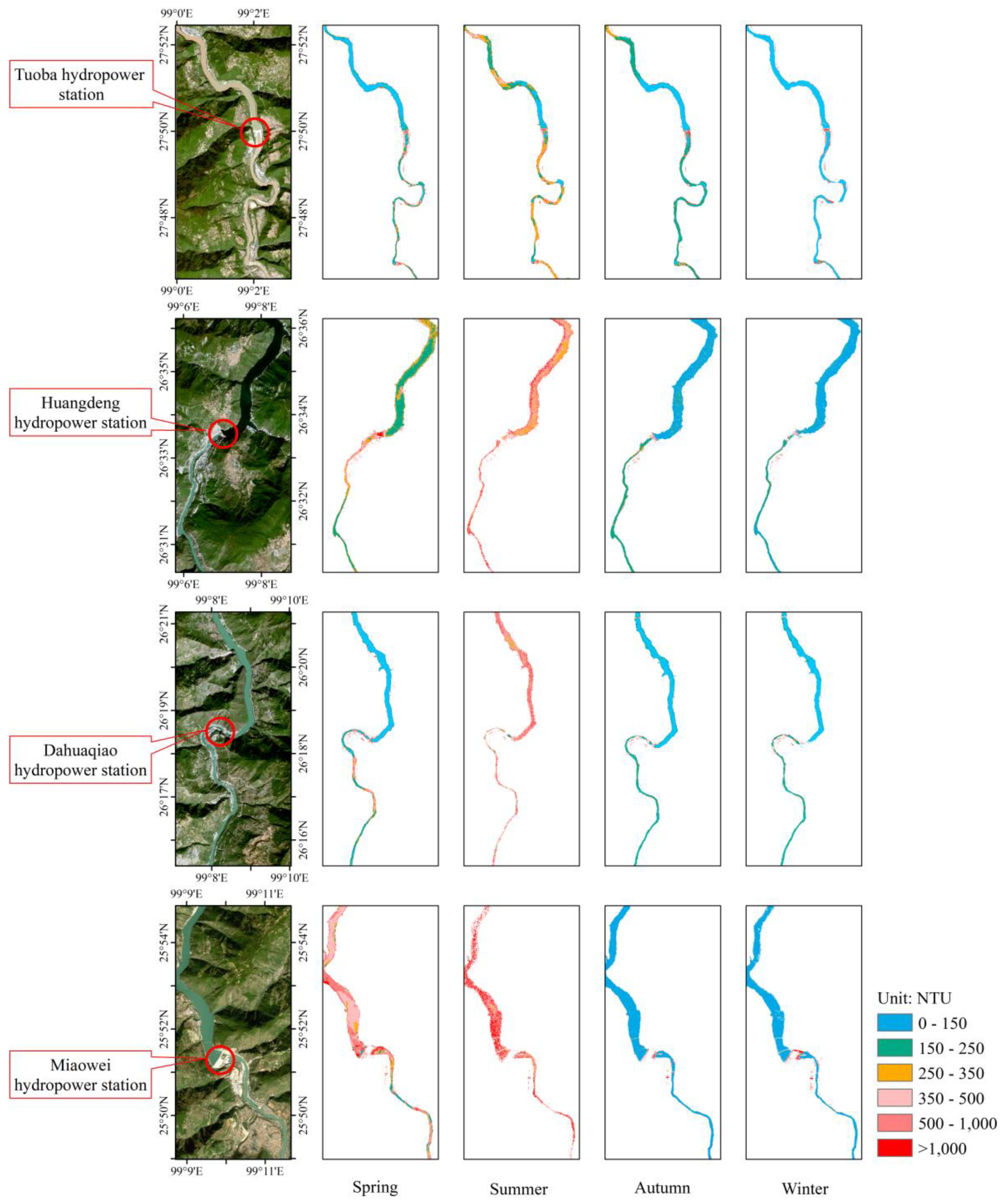
The 2BSAT model was used to analyze the temporal–spatial variation of TU based on the Sentinel-2 and Landsat series images. In the spatial variations, the five rivers showed different spatial distribution characteristics and the distribution difference of turbidity also existed upstream and downstream of the same river. In the temporal variations, it proved to be a general rule that the highest turbidity in these alpine rivers usually appeared in summer, while the lowest appeared in winter. In addition, the study found that the turbidity of KDR and YZR showed downward trends overall over the past 30 years.

(4)

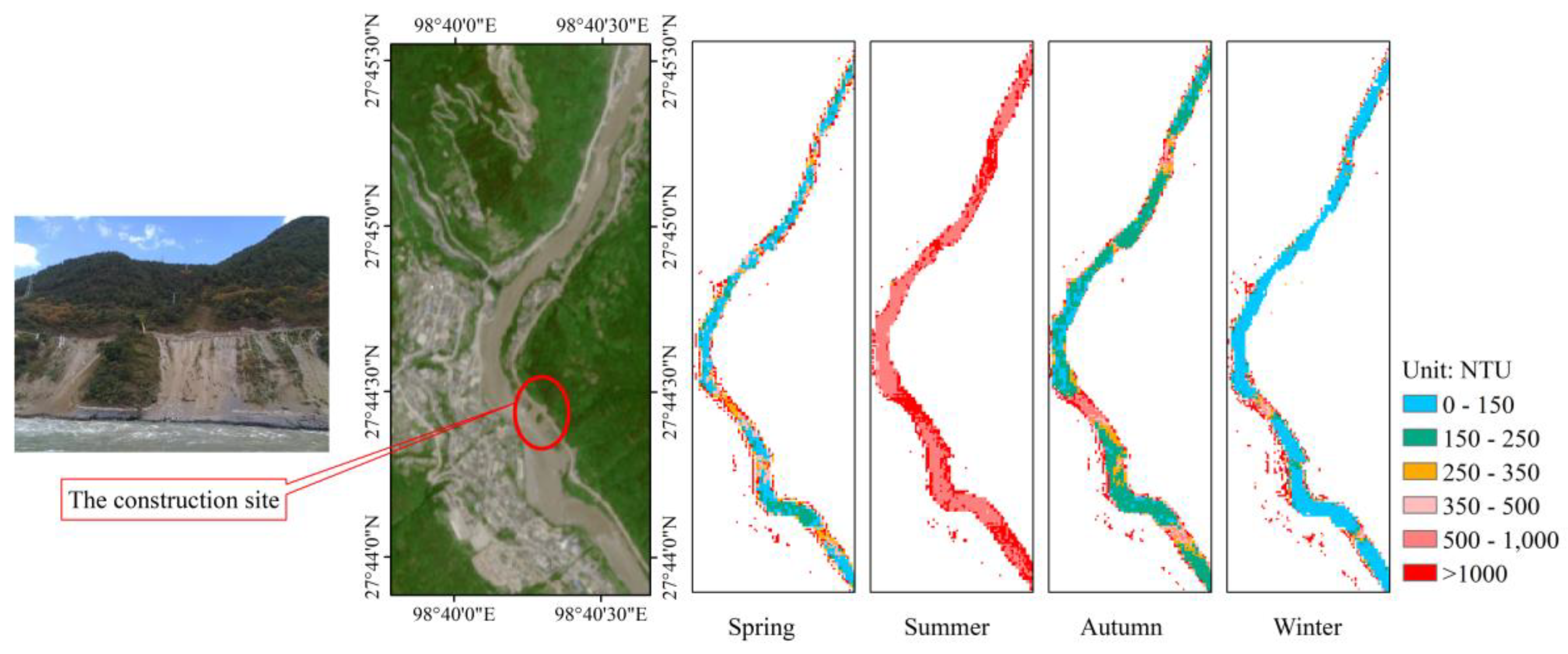
Human activities, such as engineering construction and sewage discharge, have severely affected the water quality of alpine rivers. However, seasonal factors still dominate river turbidity changes from the perspective of long river reaches. For instance, precipitation and turbidity had a consistent seasonal dynamic regularity from 1989 to 2012 and the correlation coefficient between the two reached 0.74.

References

1. Cloern, J.E. Turbidity as a control on phytoplankton biomass and productivity in estuaries. Cont. Shelf Res. 1987, 7, 1367–1381. [Google Scholar] [CrossRef]
2. Fisher, T.R.; Gustafson, A.B.; Sellner, K.; Lacouture, R.; Haas, L.W.; Wetzel, R.L.; Magnien, R.; Everitt, D.; Michaels, B.; Karrh, R.; et al. Spatial and temporal variation of resource limitation in Chesapeake Bay. Mar. Biol. 1999, 133, 763–778. [Google Scholar] [CrossRef]
3. Bilotta, G.S.; Brazier, R.E. Understanding the influence of suspended solids on water quality and aquatic biota. Water Res. 2008, 42, 2849–2861. [Google Scholar] [CrossRef] [PubMed]
4. Wang, S.Y.; Shen, M.; Ma, Y.X.; Chen, G.S.; You, Y.F.; Liu, W.H. Application of Remote Sensing to Identify and Monitor Seasonal and Interannual Changes of Water Turbidity in Yellow River Estuary, China. J. Geophys. Res. 2019, 124, 4904–4917. [Google Scholar] [CrossRef]
5. Su, B.; Ma, Y.; Menenti, M.; Wen, J.; Sobrino, J.; He, Y.; Li, Z.L.; Tang, B.; Sneeuw, N.; Zhong, L.; et al. Concerted Earth Observation and Prediction of Water and Energy Cycles in the Third Pole Environment (CEOP-TPE). In Proceedings of the Dragon 3 Final Results and Dragon 4 Kick-Off, Wuhan, China, 4–8 July 2016. [Google Scholar]
6. Zhang, T.; Zhang, Y.; Xu, M.; Zhu, J.; Ning, C.; Jiang, Y.; Ke, H.; Zu, J.; Liu, Y.; Yu, G.; et al. Water availability is more important than temperature in driving the carbon fluxes of an alpine meadow on the Tibetan Plateau. Agric. For. Meteorol. 2018, 256, 22–31. [Google Scholar] [CrossRef]
7. Ming, Q.Z.; Shi, Z.T.; Zhang, H.C. The Evolution of the Landform and Environment in the Region of the Three Parallel Rivers. Trop. Geogr. 2006, 5, 119–122. [Google Scholar]
8. Gholizadeh, M.H.; Melesse, A.M.; Reddi, L. A comprehensive review on water quality parameters estimation using remote sensing techniques. Sensors 2016, 16, 1298. [Google Scholar] [CrossRef] [Green Version]
9. Koponen, S.; Attila, J.; Pulliainen, J.; Kallio, K.; Pyhalahti, T.; Lindfors, A.; Rasmus, K.; Hallikainen, M. A case study of airborne and satellite remote sensing of a spring bloom event in the Gulf of Finland. Cont. Shelf Res. 2007, 27, 228–244. [Google Scholar] [CrossRef]
10. Le, C.; Hu, C.; Cannizzaro, J.; English, D.; Muller-Karger, F.; Lee, Z. Evaluation of chlorophyll-a remote sensing algorithm for an optically complex estuary. Remote Sens. Environ. 2013, 129, 75–89. [Google Scholar] [CrossRef]
11. Tassan, S. Local algorithms using SeaWiFS data for the retrieval of phytoplankton, pigments, suspended sediment, and yellow substance in coastal waters. Appl. Opt. 1994, 33, 2369–2378. [Google Scholar] [CrossRef]
12. Nechad, B.; Ruddick, K.; Park, Y. Calibration and validation of a generic multisensor algorithm for mapping of total suspended matter in turbid waters. Remote Sens. Environ. 2010, 114, 854–866. [Google Scholar] [CrossRef]
13. Chen, J.; Quan, W.; Cui, T.; Song, Q. Estimation of total suspended matter concentration from MODIS data using a neural network model in the China eastern coastal zone. Estuar. Coast. Shelf Sci. 2015, 155, 104–113. [Google Scholar] [CrossRef]
14. Qiu, Z. A simple optical model to estimate suspended particulate matter in Yellow River Estuary. Opt. Express 2013, 21, 27891–27904. [Google Scholar] [CrossRef] [PubMed]
15. Nechad, B.; Ruddick, K.G.; Neukermans, G. Calibration and validation of a generic multisensor algorithm for mapping of turbidity in coastal waters. In Proceedings of the International Society for Optical Engineering (SPIE 2009), San Diego, CA, USA, 2–6 August 2009. [Google Scholar]
16. Chen, J.; Cui, T.; Qiu, Z.; Lin, C. A three-band semi-analytical model for deriving total suspended sediment concentration from HJ-1A/CCD data in turbid coastal waters. ISPRS-J. Photogramm. Remote Sens. 2014, 93, 1–13. [Google Scholar] [CrossRef]
17. Kuhn, C.; Aline, D.M.; Ward, N.; Loken, L.; Sawakuchi, H.O.; Kampel, M.; Richey, J.; Stadler, P.; Crawford, J.; Striegl, R.; et al. Performance of Landsat-8 and Sentinel-2 surface reflectance products for river remote sensing retrievals of chlorophyll-a and turbidity. Remote Sens. Environ. 2019, 224, 104–118. [Google Scholar] [CrossRef] [Green Version]
18. Güttler, F.N.; Niculescu, S.; Gohin, F. Turbidity retrieval and monitoring of Danube Delta waters using multi-sensor optical remote sensing data: An integrated view from the delta plain lakes to the western–northwestern Black Sea coastal zone. Remote Sens. Environ. 2013, 132, 86–101. [Google Scholar] [CrossRef] [Green Version]
19. Lopes, V.A.; Fan, F.M.; Pontes, P.R.; Siqueira, V.A.; Collischonn, W.; da Motta Marques, D. A first integrated modelling of a river-lagoon large-scale hydrological system for forecasting purposes. J. Hydrol. 2018, 565, 177–196. [Google Scholar] [CrossRef]
20. Mobley, C.D. Radiative Transfer in Natural Waters, 1st ed.; Wuhan University Press: Wuhan, China, 2009; ISBN 978-730-707-355-5. [Google Scholar]
21. Volpe, V.; Silvestri, S.; Marani, M. Remote sensing retrieval of suspended sediment concentration in shallow waters. Remote Sens. Environ. 2011, 115, 44–54. [Google Scholar] [CrossRef]
22. Gordon, H.R.; Brown, O.B.; Evans, R.H.; Brown, J.W.; Smith, R.C.; Baker, K.S.; Clark, D.K. A semianalytic radiance model of ocean color. J. Geophys. Res. Atmos. 1988, 93, 10909–10924. [Google Scholar] [CrossRef]
23. Zhongping, L.; Carder, K.L.; Keping, D. Effects of molecular and particle scatterings on the model parameter for remote-sensing reflectance. Appl. Opt. 2004, 43, 4957–4964. [Google Scholar]
24. Shen, F.; Verhoef, W.; Zhou, Y.; Salama, M.S.; Liu, X. Satellite estimates of wide-range suspended sediment concentrations in Changjiang (Yangtze) estuary using MERIS data. Estuaries Coasts 2010, 33, 1420–1429. [Google Scholar] [CrossRef]
25. Salama, M.S.; Verhoef, W. Two-stream remote sensing model for water quality mapping: 2SeaColor. Remote Sens. Environ. 2015, 157, 111–122. [Google Scholar] [CrossRef] [Green Version]
26. Rügner, H.; Schwientek, M.; Beckingham, B.; Kuch, B.; Grathwohl, P. Turbidity as a proxy for total suspended solids (TSS) and particle facilitated pollutant transport in catchments. Environ. Earth Sci. 2013, 69, 373–380. [Google Scholar] [CrossRef]
27. Katlann, R.; Nechad, B.; Ruddick, K.; Zargouni, F. Optical remote sensing of turbidity and total suspended matter in the Gulf of Gabes. Arab. J. Geosci. 2013, 6, 1527–1535. [Google Scholar] [CrossRef]
28. Loisel, H.; Mangin, A.; Vantrepotte, V.; Dessailly, D.; Dinh, D.N.; Garnesson, P.; Ouillon, S.; Lefebvre, J.P.; Mériaux, X.; Phan, T.M.; et al. Variability of suspended particulate matter concentration in coastal waters under the Mekong’s influence from ocean color (MERIS) remote sensing over the last decade. Remote Sens. Environ. 2014, 150, 218–230. [Google Scholar] [CrossRef]
29. Chen, J.; Quan, W.; Yao, G.; Cui, T. Retrieval of absorption and backscattering coefficients from HJ-1A/CCD imagery in coastal waters. Opt. Express 2013, 21, 5803–5821. [Google Scholar] [CrossRef]
30. Gohin, F.; Stanev, E. Annual cycles of chlorophyll-a, non-algal suspended particulate matter, and turbidity observed from space and in-situ in coastal waters. Ocean Sci. 2011, 7, 705–732. [Google Scholar] [CrossRef] [Green Version]
31. Luo, Y.; Doxaran, D.; Ruddick, K.; Shen, F.; Gentili, B.; Yan, L.W.; Huang, H.J. Saturation of water reflectance in extremely turbid media based on field measurements, satellite data and bio-optical modelling. Opt. Express 2018, 26, 10435–10451. [Google Scholar] [CrossRef] [Green Version]
32. Le, C.; Li, Y.; Zha, Y.; Sun, D.; Huang, C.; Lu, H. A four-band semi-analytical model for estimating chlorophyll a in highly turbid lakes: The case of Taihu Lake, China. Remote Sens. Environ. 2009, 113, 1175–1182. [Google Scholar] [CrossRef]
33. Holm-Hansen, O.; Riemann, B. Chlorophyll a Determination: Improvements in Methodology. Oikos 1978, 30, 438–447. [Google Scholar] [CrossRef]
34. Drusch, M.; Bello, U.D.; Carlier, S.; Colin, O.; Fernandez, V.; Gascon, F.; Hoersch, B.; Isola, C.; Laberinti, P.; Martimort, P.; et al. Sentinel-2: ESA’s Optical High-Resolution Mission for GMES Operational Services. Remote Sens. Environ. 2012, 120, 25–36. [Google Scholar] [CrossRef]
35. The European Space Agency (ESA) Sentinel Online User Guides. Available online: https://earth.esa.int/web/sentinel/user-guides/sentinel-2-msi/document-library/-/asset_publisher/Wk0TKajiISaR/content.html (accessed on 24 October 2019).
36. Lee, Z.; Carder, K.L.; Hawes, S.K.; Steward, R.G.; Peacock, T.G.; Davis, C.O. Model for the interpretation of hyperspectral remote-sensing reflectance. Appl. Opt. 1994, 33, 5721–5732. [Google Scholar] [CrossRef] [PubMed] [Green Version]
37. Dall’Olmo, G.; Gitelson, A.A. Effect of bio-optical parameter variability on the remote estimation of chlorophyll-a concentration in turbid productive waters: Experimental results. Appl. Opt. 2005, 44, 412–422. [Google Scholar] [CrossRef] [PubMed] [Green Version]
38. Dogliotti, A.I.; Ruddick, K.G.; Nechad, B.; Doxaran, D.; Knaeps, E. A single algorithm to retrieve turbidity from remotely-sensed data in all coastal and estuarine waters. Remote Sens. Environ. 2015, 156, 157–168. [Google Scholar] [CrossRef] [Green Version]
39. Zimba, P.V.; Gitelson, A. Remote estimation of chlorophyll concentration in hyper-eutrophic aquatic systems: Model tuning and accuracy optimization. Aquaculture 2006, 256, 272–286. [Google Scholar] [CrossRef]
40. Gurlin, D.; Gitelson, A.A.; Moses, W.J. Remote estimation of chl-a concentration in turbid productive waters—Return to a simple two-band NIR-red model? Remote Sens. Environ. 2011, 115, 3479–3490. [Google Scholar] [CrossRef]
41. Gilerson, A.A.; Gitelson, A.A.; Zhou, J.; Gurlin, D.; Moses, W.; Ioannou, I.; Ahmed, S.A. Algorithms for remote estimation of chlorophyll-a in coastal and inland waters using red and near infrared bands. Opt. Express 2010, 18, 24109–24125. [Google Scholar] [CrossRef] [Green Version]
42. Roesler, C.S.; Perry, M.J. Modeling in Situ Phytoplankton Absorption Spectra from Spectral Reflectance: Effects of Spectral Backscatter, 1st ed.; Springer: Boston, MA, USA, 1992; ISBN 978-148-990-762-2. [Google Scholar]
43. Bricaud, A.; Morel, A.; Prieur, L. Absorption by Dissolved Organic Matter of the Sea (Yellow Substance) in the UV and Visible Domains. Limnol. Oceanogr. 1981, 26, 43–53. [Google Scholar] [CrossRef]
44. Binding, C.E.; Greenberg, T.A.; Bukata, R.P. The MERIS Maximum Chlorophyll Index; its merits and limitations for inland water algal bloom monitoring. J. Gt. Lakes Res. 2013, 39, 100–107. [Google Scholar] [CrossRef]
45. Wu, G.; Cui, L.; Duan, H.; Fei, T.; Liu, Y. Specific absorption and backscattering coefficients of the main water constituents in Poyang Lake, China. Environ. Monit. Assess. 2013, 185, 4191–4206. [Google Scholar] [CrossRef]
46. Gons, H.J. Optical teledetection of chlorophyll a in turbid inland waters. Environ. Sci. Technol. 1999, 33, 1127–1132. [Google Scholar] [CrossRef]
47. Smith, R.C.; Baker, K.S. Optical properties of the clearest natural waters (200-800 nm). Appl. Opt. 1981, 20, 177–184. [Google Scholar] [CrossRef] [PubMed]
48. Chinese Standards for Drinking Water Quality. Available online: http://www.nhc.gov.cn/wjw/pgw/201212/33644.shtml (accessed on 27 October 2019).
49. Hestir, E.L.; Brando, V.; Campbell, G.; Dekker, A.; Malthus, T. The relationship between dissolved organic matter absorption and dissolved organic carbon in reservoirs along a temperate to tropical gradient. Remote Sens. Environ. 2015, 156, 395–402. [Google Scholar] [CrossRef]
50. Nechad, B.; Ruddick, K.; Schroeder, T.; Oubelkheir, K.; Blondeau-Patissier, D.; Cherukuru, N.; Brando, V.; Dekker, A.; Clementson, L.; Banks, A.C.; et al. CoastColour Round Robin datasets: A database to evaluate the performance of algorithms for the retrieval of water quality parameters in coastal waters. Earth Syst. Sci. Data 2015, 8, 173–258. [Google Scholar] [CrossRef] [Green Version]
51. Gitelson, A.A.; Gurlin, D.; Moses, W.J.; Barrow, T. A bio-optical algorithm for the remote estimation of the chlorophyll-a concentration in case 2 waters. Environ. Res. Lett. 2009, 4, 045003. [Google Scholar] [CrossRef]
52. Matsushita, B.; Wei, Y.; Yu, G.; Oyama, Y.; Yoshimura, K.; Fukushima, T. A hybrid algorithm for estimating the chlorophyll-a concentration across different trophic states in Asian inland waters. ISPRS-J. Photogramm. Remote Sens. 2015, 102, 28–37. [Google Scholar] [CrossRef] [Green Version]
53. Du, C.; Wang, Q.; Li, Y.; Lyu, H.; Zhu, L.; Zheng, Z.; Wen, S.; Liu, G.; Guo, Y. Estimation of total phosphorus concentration using a water classification method in inland water. Int. J. Appl. Earth Obs. Geoinf. 2018, 71, 29–42. [Google Scholar] [CrossRef]
54. Gilerson, A.; Zhou, J.; Hlaing, S.; Ioannou, I.; Schalles, J.; Gross, B.; Moshary, F.; Ahmed, S. Fluorescence component in the reflectance spectra from coastal waters. Dependence on water composition. Opt. Express 2007, 15, 15702–15721. [Google Scholar] [CrossRef]
55. Gitelson, A.; Merzlyak, M.N. Spectral Reflectance Changes Associated with Autumn Senescence of Aesculus hippocastanum L. and Acer platanoides L. Leaves. Spectral Features and Relation to Chlorophyll Estimation. J. Plant Physiol. 1994, 143, 286–292. [Google Scholar] [CrossRef]
56. Palmer, S.C.; Hunter, P.D.; Lankester, T.; Hubbard, S.; Spyrakos, E.; Tyler, A.N.; Présing, M.; Horváth, H.; Lamb, A.; Balzter, H.; et al. Validation of Envisat MERIS algorithms for chlorophyll retrieval in a large, turbid and optically-complex shallow lake. Remote Sens. Environ. 2015, 157, 158–169. [Google Scholar] [CrossRef] [Green Version]
57. Bailey, S.W.; Werdell, P.J. A multi-sensor approach for the on-orbit validation of ocean color satellite data products. Remote Sens. Environ. 2006, 102, 12–23. [Google Scholar] [CrossRef]
58. Pahlevan, N.; Chittimalli, S.K.; Balasubramanian, S.V.; Vellucci, V. Sentinel-2/Landsat-8 product consistency and implications for monitoring aquatic systems. Remote Sens. Environ. 2019, 220, 19–29. [Google Scholar] [CrossRef]
59. Lathrop, R.G.; Lillesand, T.M.; Yandell, B.S. Testing the utility of simple multi-date Thematic Mapper calibration algorithms for monitoring turbid inland waters. Int. J. Remote Sens. 1991, 12, 2045–2063. [Google Scholar] [CrossRef]
60. Doxaran, D.; Cherukuru, R.C.; Lavender, S.J. Use of reflectance band ratios to estimate suspended and dissolved matter concentrations in estuarine waters. Int. J. Remote Sens. 2005, 26, 1763–1769. [Google Scholar] [CrossRef]
61. Gitelson, A.A.; Dall’Olmo, G.; Moses, W.; Rundquist, D.C.; Barrow, T.; Fisher, T.R.; Gurlin, D.; Holz, J. A simple semi-analytical model for remote estimation of chlorophyll-a in turbid waters: Validation. Remote Sens. Environ. 2008, 112, 3582–3593. [Google Scholar] [CrossRef]
62. Bowers, D.G.; Binding, C.E. The optical properties of mineral suspended particles: A review and synthesis. Estuar. Coast. Shelf Sci. 2006, 67, 219–230. [Google Scholar] [CrossRef]
63. Wu, F.; Xuan, W.; Cai, Y.; Li, C. Spatiotemporal analysis of precipitation trends under climate change in the upper reach of Mekong River basin. Quat. Int. 2016, 392, 137–146. [Google Scholar] [CrossRef] [Green Version]
64. Dong, Z.R. Ecological impacts of hydropower development on the Nujiang River, China. Acta Ecol. Sin. 2005, 26, 1591–1596. [Google Scholar]
65. Gong, L.; Li, J.; Yang, Q.; Wang, S.; Ma, B.; Peng, Y. Biomass characteristics and simultaneous nitrification–denitrification under long sludge retention time in an integrated reactor treating rural domestic sewage. Bioresour. Technol. 2012, 119, 277–284. [Google Scholar] [CrossRef]
Figure 1. Location of the three study areas. (a) The Kaidu River basin; (b) The Yarlung Zangbo River basin; and, (c) The Three Parallel Rivers basin.
Remotesensing 11 03010 g001
Figure 2. Measuring instrument and Spectrometric method. (a) HORIBA multi-parameter water quality meter U-50; (b) ASD FieldSpec Spectroradiometer; (c) Above-surface observation method [32], where θ v is the angle between the observing plane and water surface, and the range of θ v is 30–150°; φ v is the angle between the observing plane and the plane of the incident radiation away from the sun, and the range of φ v is 90–135°.
Remotesensing 11 03010 g002
Figure 3. Sentinel-2A/B MSI Spectral Response Average of visible and near infrared bands [35]. The solid curve represents Sentinel-2A, and the dashed curve represents Sentinrel-2B.
Remotesensing 11 03010 g003
Figure 4. Remote sensing reflectance field measurements and photos of river bodies. (a) Hyperspectral remote sensing reflectance R r s ( λ ) ; (b) The site photos of the five river water bodies; and, (c) Typical R r s ( λ ) spectra corresponding to different turbidity.
Remotesensing 11 03010 g004
Figure 5. Optimal band selection of 2BSAT. (a) First round of stepwise calculation to confirm λ 2 ; (c) Second round of stepwise calculation to confirm λ 1 ; (e) Third round of stepwise calculation to confirm new λ 2 ; (b,d,f): correlation the 2BSAT model of each round of stepwise calculation and the in situ turbidity.
Remotesensing 11 03010 g005
Figure 6. Comparison of modelled turbidity with in situ turbidity while using the Three Parallel Rivers (TPR) data.
Remotesensing 11 03010 g006
Figure 7. Model validation: comparison of modelled turbidity with in situ turbidity using field data from the YZR (a,b) and Kaidu River (KDR) (c,d).
Remotesensing 11 03010 g007
Figure 8. Calibration of 2BSAT using simulated Sentinel-2A datasets in TPR. (a) Correlation between the 2BSAT model and in situ turbidity; and, (b) Modelled turbidity versus in situ turbidity.
Remotesensing 11 03010 g008
Figure 9. Validation of 2BSAT using simulated Sentinel-2A datasets in KDR (a,b) and Yarlung Zangbo River (YZR) (c,d).
Remotesensing 11 03010 g009
Figure 10. Satellite-based remote sensing reflectance versus simulated remote sensing reflectance in TPR (a) and KDR (c) and modelled turbidity versus in situ turbidity in TPR (b) and KDR (d).
Remotesensing 11 03010 g010
Figure 11. Typical temporal-spatial distribution of turbidity in TPR.
Remotesensing 11 03010 g011
Figure 12. Typical temporal-spatial distribution of turbidity in KDR.
Remotesensing 11 03010 g012
Figure 13. Typical temporal–spatial distribution of turbidity in YZR.
Remotesensing 11 03010 g013
Figure 14. Seasonal change trends of turbidity in five rivers from 1989 to 2018 in JSR (a), LCR (b), NJR (c), KDR (d), and YZR (e). The dashed line indicates the variation trend of turbidity.
Remotesensing 11 03010 g014
Figure 15. In situ turbidity versus modelled turbidity by Lathrop (a), Chen (b), Nechad (c), and Doxaren (d) models.
Remotesensing 11 03010 g015
Figure 16. Relative error distributions of the five models.
Remotesensing 11 03010 g016
Figure 17. Spatial distribution of seasonal turbidity in Tuoba, Huangdeng, Dahuaqiao, and Miaowei hydropower station areas.
Remotesensing 11 03010 g017
Figure 18. Spatial distribution of seasonal turbidity in a residential quarter and road construction site.
Remotesensing 11 03010 g018
Figure 19. Comparison of variation trend of precipitation and turbidity in YZR.
Remotesensing 11 03010 g019
Figure 20. The correlation between precipitation and turbidity in YZR.
Remotesensing 11 03010 g020