Article

Mapping Spatial Variations of Structure and Function Parameters for Forest Condition Assessment of the Changbai Mountain National Nature Reserve

1
Key Laboratory of Wetland Ecology and Environment, Northeast Institute of Geography and Agroecology, Chinese Academy of Sciences, Changchun 130102, China
2
University of Chinese Academy of Sciences, Beijing 100049, China
3
Department of Natural Resources Science, University of Rhode Island, Kingston, RI 02881, USA
4
National Earth System Science Data Center, Beijing 100101, China
*
Authors to whom correspondence should be addressed.
Remote Sens. 2019, 11(24), 3004; https://doi.org/10.3390/rs11243004
Submission received: 19 October 2019 / Revised: 21 November 2019 / Accepted: 9 December 2019 / Published: 13 December 2019
(This article belongs to the Special Issue Remote Sensing Applications in Monitoring of Protected Areas)

Abstract

:
Forest condition is the baseline information for ecological evaluation and management. The National Forest Inventory of China contains structural parameters, such as canopy closure, stand density and forest age, and functional parameters, such as stand volume and soil fertility. Conventionally forest conditions are assessed through parameters collected from field observations, which could be costly and spatially limited. It is crucial to develop modeling approaches in mapping forest assessment parameters from satellite remote sensing. This study mapped structure and function parameters for forest condition assessment in the Changbai Mountain National Nature Reserve (CMNNR). The mapping algorithms, including statistical regression, random forests, and random forest kriging, were employed with predictors from Advanced Land Observing Satellite (ALOS)-2, Sentinel-1, Sentinel-2 satellite sensors, digital surface model of ALOS, and 1803 field sampled forest plots. Combined predicted parameters and weights from principal component analysis, forest conditions were assessed. The models explained spatial dynamics and characteristics of forest parameters based on an independent validation with all r values above 0.75. The root mean square error (RMSE) values of canopy closure, stand density, stand volume, forest age and soil fertility were 4.6%, 33.8%, 29.4%, 20.5%, and 14.3%, respectively. The mean assessment score suggested that forest conditions in the CMNNR are mainly resulted from spatial variations of function parameters such as stand volume and soil fertility. This study provides a methodology on forest condition assessment at regional scales, as well as the up-to-date information for the forest ecosystem in the CMNNR.

Graphical Abstract

1. Introduction

Forests occupy almost one third of the Earth’s land area [1], playing a major role in sustaining global material and energy cycles [2]. Forests provide a variety of ecosystem services, which are important for human well-being and the overall health of the planet Earth [3,4]. Forest condition is an essential component of both forest management and ecological evaluations. It reflects the stability, resilience, and capability of carbon sequestration, timber production, as well as other services [5,6]. Current forest condition assessments are mainly based on the structure and function investigated in the field, which is costly and spatially limited [7]. It is essential to assess forest condition based on modeling structural and functional parameters. The condition assessment based on remote sensing usually contains indicators of community structure and productivity [6,7,8]. The sub-compartment measurements of the National Forest Inventory in China contain the information about structure, including canopy closure, stand density and forest age, and function, including stand volume and soil condition [9,10].
The explicit mapping of spatial variations of forest structure and function parameters has been an essential effort in ecological analysis [11,12,13,14]. Remote sensing modeling combined sample plot data has become a well adopted method to generate spatially explicit estimates of forest parameters [15,16]. The selection of predictor variables from various sensors and algorithms can affect the results considerably [17,18]. Variables from optical sensors are commonly applied to predict horizontal forest structure such as canopy closure and density [19,20]. This is due to the close relationship between horizontal forest structure and aggregate spectral signatures, i.e., reflectance or vegetation indices, with global coverage, repetitiveness, and cost-effectiveness [21,22]. However, synthetic aperture radar (SAR) and light detection and ranging (LiDAR) sensors are capable of penetrating cloud and canopies and are suitable for mapping vertical forest parameters such as tree height and stand volume [23,24,25]. Whereas, complex forest parameters such as biomass, soil fertility, and forest age are generally estimated by multi-sensor data [26,27,28,29].
Modeling vegetation parameters based on remote sensing can be divided into physically based models and empirical regression algorithms [18,21,30]. Physically based models depend on numerous factors to simulate canopy reflectance, such as leaf geometry, chlorophyll concentration, water and matter contents, soil reflectance, and bidirectional reflectance distribution function, which may not be readily available [31,32]. Those are built conventionally as semi-physical models by simplifying factors based on prerequisite assumptions and using machine learning or regression methods trained with radiative transfer, which achieve robust performance [33,34]. The biophysical products, such as leaf area index (LAI) and fraction of vegetation cover (FVC) from Sentinel-2, are generated by a physically based model, which has been implemented to Moderate Resolution Imaging Spectrometer (MODIS) and Landsat sensors [35,36]. Empirical regressions require support from abundant ground measurements, and depend on the modeling relationship between remote sensing-derived predictors and field-measured samples, including parametric and non-parametric algorithms [37,38]. The former refers to statistical regression methods, by which the expression relating to the dependent variable, i.e., forest parameters, and the independent variables are estimated [39,40]. These regressions are suitable to model explicit relationships and are easily applied to a large scale [12,41,42]. As for the complex forest parameters such as stand volume, forest age, and soil fertility, it is a challenge to formulate their relationships with remote sensing data because of many affecting factors [43,44,45] which require non-parametric algorithms. Among the various non-parametric techniques, random forests (RF) has been recognized to be efficient and accurate in modeling complex relationships between remote sensing data and forest parameters [7,17,46,47].
Forest parameter modeling based on satellite data has advantages such as repetition rate enabling long-term monitoring [48,49]. Sentinel-1 C band SAR and Sentinel-2 multispectral instrument (MSI) have the global coverage [50]. Those publicly accessible data have been applied in vegetation studies and provided capabilities for forest parameter modeling using both active and passive remote sensing techniques [51,52]. The Advanced Land Observing Satellite (ALOS/ALOS-2) Phased Array type L band SAR (PALSAR/PALSAR-2) images from L band SAR contain comprehensive information on the orientation and structure of tree canopy and stems within the pixel [53,54,55]. It makes the yearly mosaic ALOS/ALOS-2 images with global and free-access observations particularly useful for forest parameter mapping [56,57]. The digital surface model (DSM) from ALOS L band interferometric SAR (InSAR) had greater accuracy and can provide useful topographic indices to estimate forest parameters [58,59]. Although estimates of forest parameters from moderate resolution satellite images and abovementioned algorithms have achieved varying success [12,13,49], inventory and application of efficient algorithms and predictors from open-access remote sensing data on forest structure, function, and condition assessment continuously deserve exploration.
The Changbai Mountain National Nature Reserve (CMNNR) in Northeast China is covered with large areas of old-growth forests, which are under strict protection [60,61]. It has been regarded as the most typical natural composite body on the Eurasia Continent with a complex biota composition and abundant flora and fauna [62,63]. Due to its ecological importance, substantial researches on landscape structure, function, and productivity in the Changbai Mountain region have been reported since the early 1980s [64,65,66,67,68,69]. However, there is a lack of systematic maps of forest parameters and conditions in this vital ecosystem site.
In this study, we developed an effective methodology for evaluating forest conditions by mapping canopy closure, stand density, volume, age, and soil fertility in the CMNNR. The specific objectives were to: (1) model forest structure and function parameters by determining their relationships with predictors from satellite data, including L and C band SAR, topographical indices from L band InSAR, and Sentinel-2 MSI variables; (2) map five parameters using efficient algorithms with remote sensing data; and (3) assess forest conditions based on structural and functional parameters, which can provide baseline information for forest management.

2. Materials and Methods
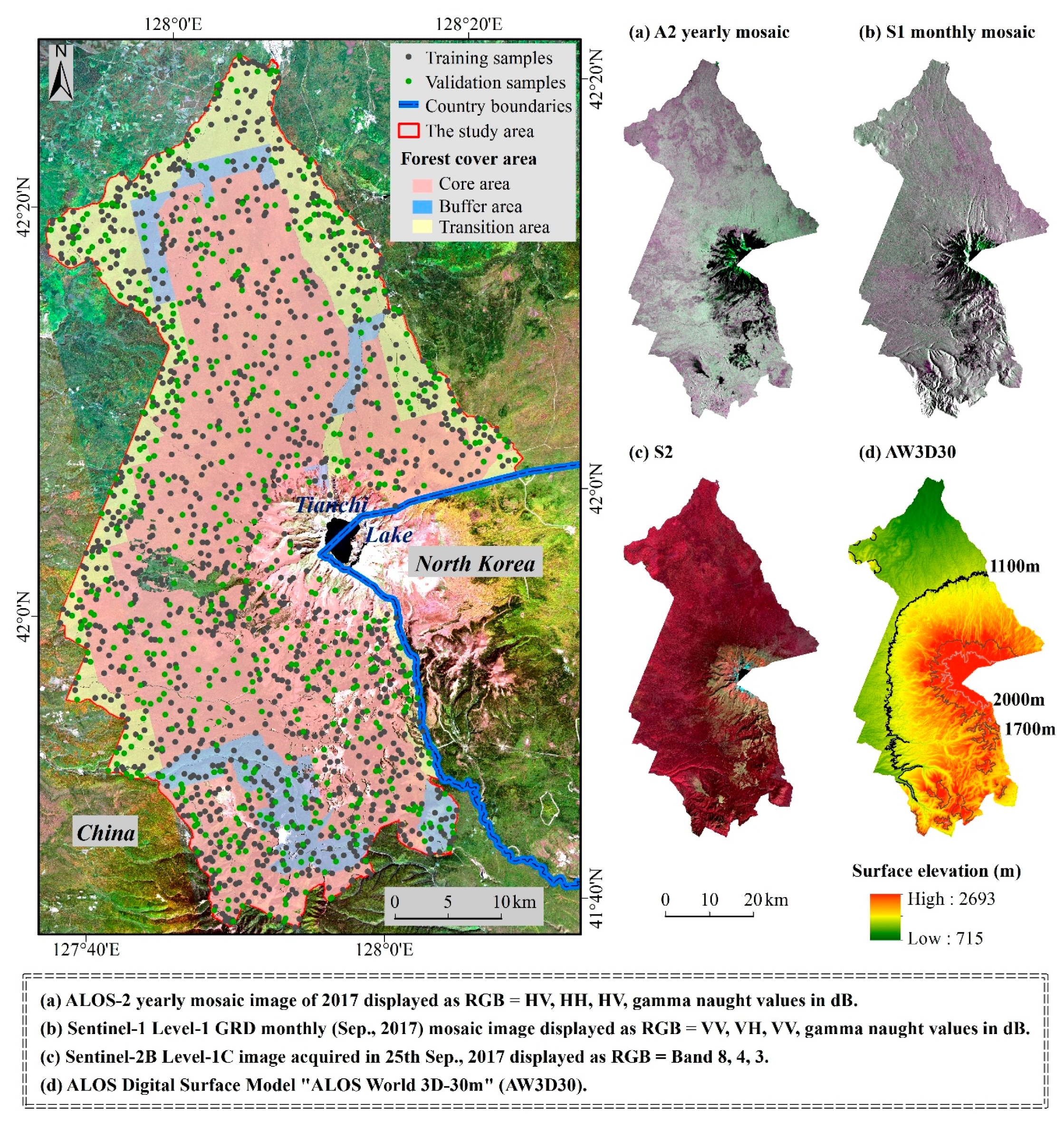
2.1. Study Area

The CMNNR (41°42′–42°25′N, 127°42′–128°17′E) was established in 1961. It is located in Jilin Province of northeastern China (Figure 1). The top of the reserve is a volcanic summit cupping a crater lake named Tianchi at 2693 m above sea level on the China-North Korea border. The reserve occupies an area of 195,852 ha in the Chinese side. It has the largest protected temperate forests which supports a significant species gene base and biodiversity in Northeast Asia. The CMNNR was admitted into the United Nations Educational, Scientific, and Cultural Organization’s (UNESCO’s) Man and Biosphere Program in 1979 [70]. This site has a continental temperate climate characterized by a long cold winter and short cool summers with recognizable vertical climate and vegetation zones. The annual average precipitation and temperature range from 700 to 1400 mm and −7 °C to 3 °C, respectively. This area has dense forests covered 177,082 ha (90.4%). The forests in the reserve are divided into three functional management zones including the core, buffer, and transition areas [71]. Harvesting and poaching are prohibited in the core area. The human disturbances are prevented from the core area by the buffer zone. The endemic species, ecotourism, and bases for reproduction of natural resources are established in the transition area. From the foot of the mountain to the peak, vegetation changes in distinguishable vertical zones with elevation. The distributions include mixed coniferous and broad-leaved forest (<1100 m), dark-coniferous spruce-fir forest (1100–1700 m), Ermans birch forest (1700–2000 m), and alpine tundra (>2000 m) [72]. Soils also differ in each vertical zone, typically marked by dark-brown and brown earths, meadow, volcanic, bog, and bleached baijiang soil.

2.2. Data

2.2.1. Field Data

The field campaign was carried out from the end of August to the beginning of October in 2017. The stratified sampling design was adopted. Non-forest areas were masked out and the distribution of sampling plots was randomly generated in forest areas, while the plot sites which were impossible to access were replaced by the nearest sites. Following the national guidelines for forest resource survey [73], ten teams took part in the field campaign and collected measured data under the same protocol. A total of 1803 30 m by 30 m plots were located and sampled (Figure 1). At each sample site, tree species, diameter at breast height (DBH, the diameter at 1.3 m from the ground), tree height, soil depth and types, as well as the number of trees, were measured and recorded. Overhead photos of the canopy by fisheye lens were taken at the center of each sample site. The measured parameters were acquired based on field sample sites and processes shown in Table 1. Stand volume of each sample was estimated by DBH and tree height according to the National Standard of China: Tree volume tables (LY/T 1353–1999) [74]. Canopy closure was estimated from fisheye photos after processing of circle clipping, binary conversion, and raster calculation [75]. Soil fertility was assessed by the depth weighted according to soil types as shown in Table 1. The six types of soils in the study area were assigned three different weights based on previous studies of their organic carbon density [76,77]. The descriptive statistics of field-based forest parameters were shown in Table 2. The 1803 sample sites were randomly split into training (n = 1202) and validation (n = 601) sets (Figure 1) for modeling and validating the spatial variation of forest parameters, respectively.

2.2.2. Remote Sensing Data

In this study, 18 predictor variables related to forest parameters were selected and extracted from multi-sensors imagery (Table 3 and Table 4) [12,78,79,80]. ALOS-2 PALSAR-2 yearly mosaic image of 2017 was masked and converted to gamma naught values in decibel unit (dB) from 16-bit digital number (DN) (Table 4) using the following equation [81]:
γ 0   =   10 log 10 ( D N 2 ) 83
where γ 0 is gamma naught backscatter coefficient of horizontal transmit-horizontal channel (HH) or horizontal transmit-vertical channel (HV); DN is the polarization data in HH or HV.
Monthly mosaic predictors from C band SAR were generated from seven Sentinel-1 Ground Range Detected images by masking and mosaic using Google Earth Engine (GEE). Those data were pre-processed by thermal noise removal, radiometric calibration, and terrain correction stored in dB via log scaling [82]. The cloud-free Sentinel-2B Level-1C images acquired on 25 September 2017 were downloaded from the Copernicus Sentinel Scientific Data Hub (https://scihub.copernicus.eu/) to extract vegetation and soil indices, as well as biophysical variables. Previous studies explored numerous Sentinel-2 spectral indices. They found that four vegetation indices and two soil indicators were useful in modelling forest age and soil fertility, respectively [78,80,83,84,85]. The MSI data had 13 spectral bands with 10 m (bands 2–4, 8), 20 m (band 5–7, 8a, 11–12), and 60 m (band 1, 9–10) spatial resolutions. Bottom-of-atmosphere-corrected reflectance (Level-2A) images were atmospherically corrected from the Level-1C data by SEN2COR atmospheric correction processor based on the radiative transfer model (version 2.5.5, European Space Agency, Paris, France). Then, eight predictors were acquired by resampling, band math, biophysical processor, and mosaic from Level-2A images based on SNAP software (version 6.0, European Space Agency).
The DSM data from ALOS as AW3D30 were download from Japan Aerospace Exploration Agency (https:ww.eroc.jaxa.jp/ALOS/en/aw3d30/data/index/htm) to extract topographic indices based on Spatial Analyst of ArcGIS software (version 10.0, ESRI, RedLands, CA, USA). All predictor data were re-projected into UTM Zone 52 WGS84, and then resampled to the 30 m pixel size by ArcGIS.

2.3. Assessment of Forest Conditions

2.3.1. Spatial Modeling of Canopy Closure and Stand Density by Statistical Regressions

Stand density is a prominent component of forest structure, which governs elemental processing and retention, competition, and habitat suitability [86,87]. Canopy closure is the proportion of the sky hemisphere occupied by tree crowns when viewed from a single ground point [88,89]. It is closely associated with understory light and has wide-reaching effects for ecological processes in forests [90]. Whereas FVC is defined as the percentage of the forest area covered by the vertical projection of trees [91,92]. LAI is one half of the total green leaf area per unit ground surface area [93]. FVC and LAI are critical biodiversity variables as recognized by international organizations such as Global Climate Observation System and Global Terrestrial Observation System [35]. The generalized linear correlations were discovered between stand density and LAI, canopy closure and FVC, and LAI and FVC in previous studies [42,94,95]. Thus, it was assumed in this study that canopy closure and stand density could be modeled by generalized linear regressions based on FVC and LAI from Sentinel-2 images. In this study, five types of regression models (linear, quadratic polynomial, power, exponential, and logarithmic) were built. LAI or FVC, and canopy closure or stand density, were used as the input variables to derive the empirical parameters for the models. This study selected the model with the largest value of coefficient of determination (R2) to map the canopy closure and stand density.

2.3.2. Spatial Modeling of Stand Volume and Forest Age by Random Forests

Firstly, a semi-physical simple water cloud model (WCM) was used for the investigation of the relationship between stand volume and backscatters (HH and HV) derived from ALOS-2 data. The prerequisite assumption of WCM was that the dielectric constant of dry vegetation matter was much smaller than that of the water content of vegetation, and almost all volume backscatters were composed of air in the vegetation canopy [96]. Therefore, WCM was developed assuming that the canopy “cloud”, called the water cloud, contained identical water droplets showed the random distribution within the canopy [55]. In this study, the WCM was adopted for the initial exploration [97], which was written as Equation (2):
γ f 0   =   γ g 0 e δ SV   +   γ v 0 ( 1 e δ S V )
where γ f 0 is the backscatter from the forest, as the gamma naught value of HH or HV (dB); γ g 0 is the direct backscatter from the forest floor through gaps in the canopy (dB); γ v 0 is the volume backscatter from an opaque canopy without gaps (dB); SV is stand volume (m3/ha); and δ is the extinction coefficient.
Then, RF was used to model the spatial distribution of stand volume with predictors of HH and HV. The RF was an ensemble of decision trees, which was created by a subset of training sample through replacement as a bagging approach [98]. Each decision tree was independently developed without any pruning and each node was divided using a user-defined number of features selected at random [99]. By producing the forest up to a user-defined number of trees, RF creates trees with large variance and small bias [98,99]. The abovementioned two user-defined parameters, i.e., numFeatures and numIterations, were selected by the smallest root mean square error (RMSE) in WEKA software (version 3.8, The University of Waikato, Hamilton, New Zealand), and the attribute importance was also estimated [100]. The new unlabeled data were input to evaluate and vote, and the finial prediction was the average of the membership (Figure 2a). Additionally, forest age, as indirect and complex retrieved parameters for remote sensing techniques, was also modeled by RF with multi-sensor predictors (Table 4 and Figure 3).

2.3.3. Spatial Modeling of Soil Fertility by Random Forest Kriging

Random forest kriging (RFK) was the extension of RF, which integrated RF prediction values and estimation of the residuals by ordinary kriging (OK) using Equation (3) [101]. It considered spatial parametric non-stationarity with the effects of environmental variables derived from the benefits of RF [102,103]. RFK also added the spatial dependence of the residuals interpolated through OK to the estimated trend, as part of the spatial autocorrelation. RFK has been conducted in soil attribute mapping and had a greater accuracy than RF [104,105]. Its implementation included two steps (Figure 2). First, RF was used to model the relationship between soil fertility and multi-sensor predictors. Second, the result of RFK was predicted as the sum of the RF result and its residuals interpolated by the OK approach using Equation (4).
S F R F K   =   S F R F   +   R O K
{ R O K   = i = 1 n ω i R i i = 1 n ω i   =   1  
where S F R F K , S F R F are predication of soil fertility based on RFK and RF, respectively; R OK is the estimated residuals of soil fertility from RF models; Ri is the residuals of soil fertility from RF models at a measured sample i; w i is the weight estimated by the stationary OK system as an error variance model to minimize the error from the semivariogram modeling [106]; and n is the number of measured values within a neighborhood.

2.3.4. Model Evaluation and Forest Condition Assessment

The validation set (Figure 1) was used to test performances of spatial modeling of forest parameters based on the root mean squared error (Equation (5)), mean absolute error (MAE, Equation (6)), mean error (ME, Equation (7)), and correlation coefficient between the measured and predicted parameters (r, Equation (8)). In order to better estimate accuracy, the mean measured value of the parameter ( y ¯ ) was applied to divide the RMSE, MAE, and ME (Equations (5)–(7)).
RMSE   =   1 y ¯ 1 n ( y i y ^ i ) 2 n   ×   100 %
MAE   =   1 y ¯ 1 n | y i y ^ i | n   ×   100 %
ME   =   1 y ¯ 1 n y i y ^ i n   ×   100 %
r   = 1 n ( y i y ¯ ) ( y ^ i y ^ ¯ ) 1 n ( y i y ¯ ) 1 n ( y ^ i y ^ ¯ )
where y i is the measured parameter value; y ^ i is the predicted parameter value; y ¯ and y ^ ¯ are the average of measured and predicted values of the parameter, respectively; and n is 601 in this study. The RMSE and MAE should be as small as possible. The ME should be close to zero, while r should be larger.
After that, each map of forest parameters was transformed into the spatial distribution of the parameter score as Equation (9). All parameters were positive indicators for forest condition, except that stand density was considered as a complex indicator. Indeed, excessive or insufficient stand density was harmful to forest conditions [107]. In this study, optimum stand density for forest condition was assigned as the median of measured values (500 tree/ha in Table 2). In other words, stand density below 500 tree/ha was regarded as a positive parameter along with canopy closure, stand volume, forest age, and soil fertility. While stand density above 500 tree/ha was regarded as a negative parameter.
Score j   = { P i P min P max P min × 100 ,   P   is ,   CC ,   SV ,   FA ,   SF   or   SD 500   P max P i P max P min × 100 ,   P   is   SD > 500  
where Score j is the score of parameter j; P i , P min , and P max are raw data, minimum, and maximum values of spatial modeled parameters, respectively; CC, SV, FA, SF, and SD are canopy closure, stand volume, forest age, soil fertility, and stand density, respectively.
To estimate quantitatively the weight of each parameters, the principal component analysis (PCA) is a common method to use [108,109]. PCA was performed under the factor analysis in SPSS (version 21.0, IBM, Armonk, NY, USA) using Equation (10) by three elements, i.e., coefficients of parameters in linear combinations of different principal components, variance contribution rate of principal components, and normalization of weights. Finally, the forest condition assessment map was generated by the score and weight of each parameter according to Equation (11).
{ w j   =   k = 1 q C jk E k V k k = 1 q V k j = 1 5 k = 1 q C jk E k V k k = 1 q V k     j = 1 5   w j = 1     j = 1 5   V k 8
where w j is the weight of parameter j; C jk is the component matrix value of parameter j in component k; E k is eigenvalue of component k; V k is variation contribution rate of component k; and q is principal component number.
Condition score   = j = 1 5 Score j × w j
where Condition score is the score of forest condition s; Score j is the score of parameter j; and w j is the weight of parameter j.

3. Results

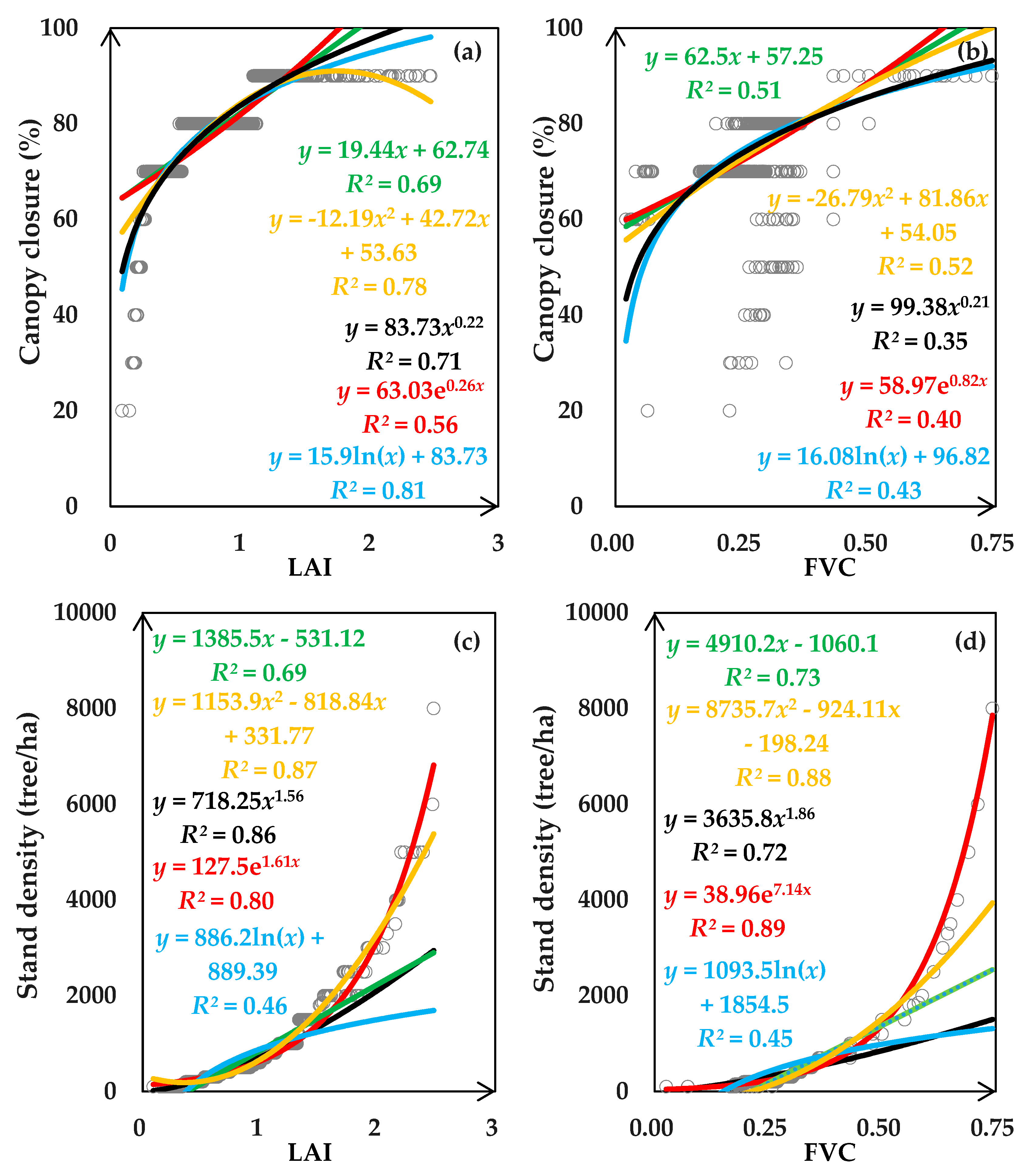
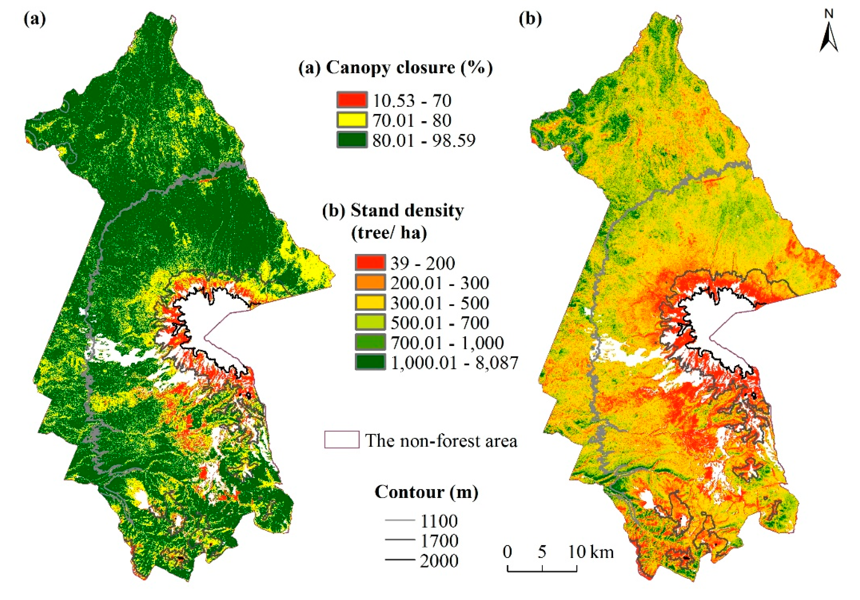
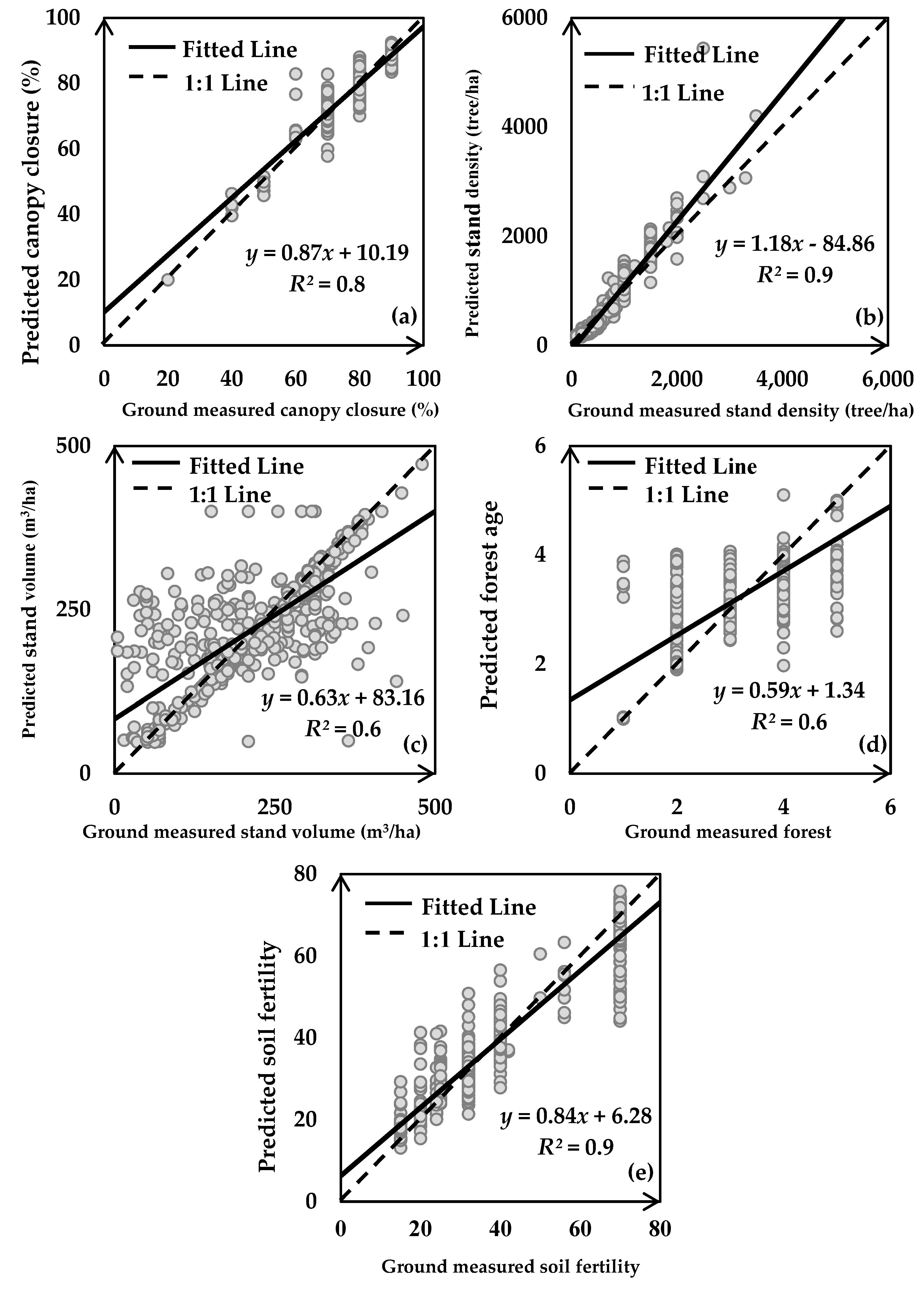
3.1. Canopy Closure and Stand Density

The five types of statistical regression models were built as illustrated in Figure 4. Among five models, logarithmic, and quadratic power regressions with the largest values of R2 were the best at explaining relationship of canopy closure with LAI and FVC, respectively. Considered the much larger R2 value of a LAI-based model, LAI derived from Sentinel-2 was selected to map canopy closure based on the logarithmic regression model. Likewise, the exponential regression model with FVC was selected to map stand density. For comparison with field measured values, the modeled output of canopy closure and stand density were divided into several levels for displaying (Figure 5). Specifically, each level had an equal number of measured sample sites. The better performance of spatial modeling of canopy closure and stand density can be indicated by the agreement pattern at each level. Generally, predicted canopy closure and stand density were close to field measured values (Table 2). The large values of canopy closure and stand density were distributed in lower altitude regions. There is no forest in the high elevation alpine tundra and the volcanic summit of the study site. The southern slope of the Changbai Mountain showed less canopy closure and stand density than the north, as affected by historical volcanic damages (Figure 5).

3.2. Stand Volume and Forest Age

The fitting line of HV showed a much flatter range than that of HH (Figure 6), indicating that HV was much more sensitive to stand volume than HH. It was also shown that the L band ALOS-2 backscatters reached saturation at around 400 m3/ha, which was greater than 97.4% of measured stand volume (Table 2). Thus, ALOS-2 data were considered suitable for spatial modeling of stand volume in the study area. Based on 1000 decision trees and one feature, the RF model was built to predict stand volume with more contribution from HV than HH. The result was depicted in Figure 7a and different levels were divided against measured values. It was delineated that the northeastern part of the study area was a large valued region.
The RF model with 1000 decision trees and six features was trained to predict forest age. The attribute importance ranking in decreasing order was H, Slope, Global environmental monitoring index (GEMI), Aspect, normalized difference vegetation index (NDVI), green normalized difference vegetation index (GNDVI), topographic wetness index (TWI), Sentinel-2 red-edge position index (S2REP), HV, Cv, Ch, VV, HH, and VH. It was indicated that topographic and vegetation indices contributed more than SAR backscatters. According to measured age, the majority of forests were mature or over-mature with a median value of four (Table 2). The predicted forest age, as Figure 7b, was consistent with the measured values. Greater values of forest age were found in the western part of the study area. It was also shown that small values of forest age and stand density in higher altitude regions where forest distribution was limited.

3.3. Soil Fertility

The RF model with 1000 decision trees and seven features was trained to predict soil fertility at the first step. The ranking of attribute importance in decreasing order was H, Slope, Aspect, Cv, Ch, TWI, second brightness index (BI2), color index (CI), HV, HH, VV, and VH. It was revealed that topographic and soil indices contributed more than SAR backscatters. By dividing into three levels against measured values, the RF-based soil fertility displayed zonal distribution (Figure 8a). The small and large values were mixed in distribution. The RF model overestimated small values while underestimating large values in comparison to measured soil fertility (Table 2). With range, nugget, and sill values of 14.5 km, 48.6, and 230.5, respectively, semivariogram in OK interpolation was modeled as an exponential type and used to predict soil fertility residuals from RF at the second step. The small value of basal effect (nugget/sill = 0.21) showed a strong autocorrelation of residuals. It was suggested that soil fertility prediction be overestimated by RF in the high-altitude area (Figure 8b). Final predicted soil fertility by RFK with more equal area of each level than RF prediction, which means closer to the measured soil fertility, was shown in Figure 8c. Soil fertility decreased as altitude increased, which agreed with vertical zonal patterns affected by the volcanic eruption hundreds of years ago.

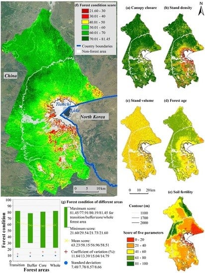
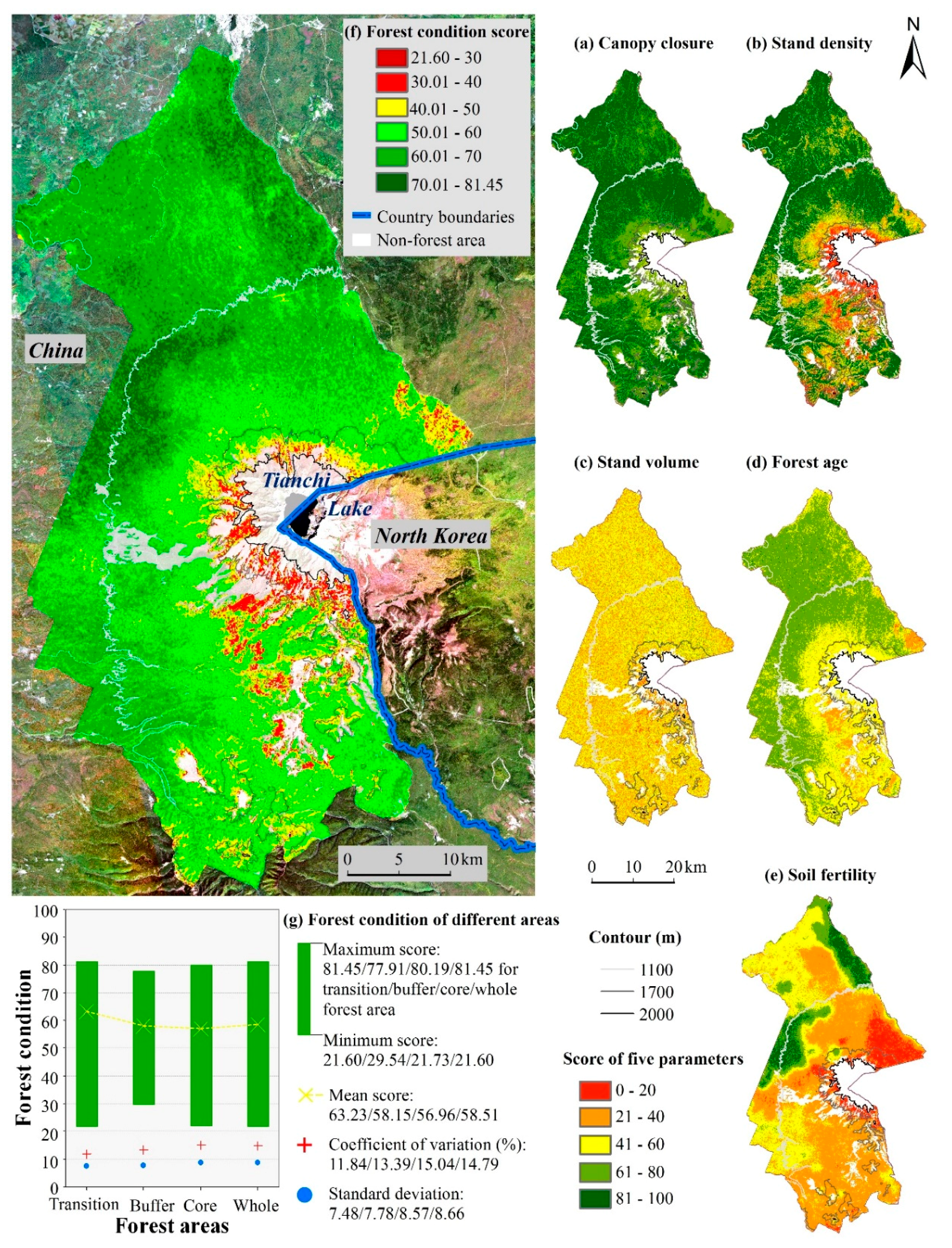
3.4. Assessment of Modeling Accuracy and Forest Condition

The spatial modeling accuracy of five forest parameters was estimated by independent data (n = 601). Canopy closure was modeled with the greatest accuracy among the five parameters, while modeling stand density performed the worst with the least accuracy (Table 5). With large values of r and R2 (r ≥ 0.75 and R2 ≥ 0.6), it was revealed that all models explained spatial dynamics and characteristics of parameters to a good extent (Figure 9). The modeled parameters were credible (r ≥ 0.75) for application in forest condition assessment.
According to PCA of measured parameters, two components were acquired and shown as Table 6. Forest age contributed the most among the five parameters with a weight of 0.23, followed by stand volume and canopy closure. Stand density had the weakest influence with a weight of 0.12. The normalized parameters scores were shown in Figure 10a–e. The largest score in canopy closure was distributed homogeneously, with almost all above 60. However, the score of soil fertility showed the strongest spatial variations, followed by that of stand density. Weighted by five parameters, forest condition score was mapped as Figure 10f. The forest of the study area in 2017 had major scores were between 50 to 70 and coefficient of variation (CV) as 14.79% (Figure 10g).

4. Discussion

4.1. Understanding Forest Parameters with Remote Sensing Predictors

Close relationships were found for canopy closure and stand density with LAI and FVC from Sentinel-2 (Figure 4). LAI explained more canopy closure (R2 = 0.81) than FVC (R2 = 0.52). However, the performances of LAI (R2 = 0.87) and FVC (R2 = 0.89) on modeling stand density were similar. The assessment by independent sample sites (Table 5 and Figure 9) showed that LAI and FVC revealed spatial variations of canopy closure and stand density (r ≥ 0.9 and R2 ≥ 0.8). While RMSE values showed that stand density was estimated with the largest error among the five parameters (Table 5). This may have resulted from the saturation problems from Sentinel-2. It was indicated that biophysical products of Sentinel-2, especially LAI, had good abilities to delineate the spatial variation of simple horizontal structure, such as canopy closure and stand density, in the study area.
The backscatter from HV was more sensitive to stand volume than HH based on the WCM models (Figure 6) and the attribute importance in the RF model. This revealed that HV backscatter was more helpful than HH to model forest productivity, which was consistent with previous findings of aboveground biomass [110,111]. The extinction coefficients modeled by WCM models in this study were much larger than previous studies in modeling aboveground biomass with backscatters and without mosaic [55,97]. This resulted in a relatively less accuracy of stand volume among five forest parameters.
The attribute importance in RF models demonstrated that topographic and spectral indices from L band InSAR and MSI contributed more than backscatters from L and C band SAR in modeling forest age and soil fertility. Additionally, backscatters from HV and VV had influenced more on forest parameter modeling than HH and VH, respectively. However, the ranking of predictor importance was different between forest age and soil fertility. The L band InSAR predictors showed the absolute dominance in soil fertility modeling, followed by variables from MSI, L band SAR, and C band SAR. This was on account of the good penetrability of L band and sensitivity to vegetation (CI) and soil humidity (BI2) of indices from MSI. As for forest age modeling, HV backscatter was much more important than second-derivative topographic micro indices (Cv and Ch). Additionally, vegetation indices from near-infrared (Band 8 and 8A), red (Band 4), vegetation red edge (Band 7), and green band (Band 3) had a greater effect than the complex macro topographic index (TWI) on forest age modeling. Also, the backscatter from VV was much more significant than that from HH. It was denoted that forest age had a more complex relationship than soil fertility with SAR and MSI data, which contained multisource influences form basic vertical and horizontal forest parameters. Moreover, the multi-sensor modeling of soil fertility based on RF algorithms showed certain limits in predicting minimum and maximum values (Figure 8a) with strongly auto-correlated residuals (nugget/sill = 0.21). It was also revealed that soil fertility had the heterogeneity conveyed by backscatters and reflectance, and the spatial autocorrelation dependence on own attributes.

4.2. Uncertainty of Spatial Modeling

The uncertainty analysis is crucial for understanding the quality of remote sensing-based forest parameters. RMSE used in this study is the common statistic to characterize the uncertainty [112,113]. Overall, the uncertainty of forest parameter modeling was acceptable with all r values above 0.75 and RMSE below 35% based on the independent validation data (Table 5). The uncertainties were from three aspects in this study as field-measurements, predictor variables and modeling. In order to get representative sample sites, a total of 1803 plots covering forests in the study area were measured (Figure 1). To match the remote sensing data, the plot size was set as 30 m by 30 m. Then, open-access remote sensing data from four different sources were selected to match the field campaign time. Predictor variables were derived from the monthly mosaic of filtered Sentinel-1 images. Limited by the cloud cover, only one cloud-free image from Sentinel-2 acquired on 25 September 2017 was used.
The forest parameters in this study were modeled with efficient predictor variables from minimum data sources based on previous findings. Specifically, canopy closure, and stand density were modeled by Sentinel-2 and stand volume was modeled by L band SAR. It was accorded from previous studies that SAR data were sensitive to vertical structure and function while MSI were primary in horizontal canopy modeling [18,21]. L band SAR penetrated into the canopy and scatters back from leaves, branches, and stems [114]. Hence, L band SAR was used to model stand volume, and DSM from L band InSAR was chosen to extract topographic indices in this study, rather than SRTM DEM from C band as most researches used. Nevertheless, as complex parameters, forest age and soil fertility were modeled by multi-sensor data to reflect the information on basic structure and function.
The uncertainty of modeling was reduced by using efficient algorithms combined with remote sensing predictors based on existing researches. First, the physically based models were considered to acquire the basic variables which were directly related to remote sensing data, such as LAI and FVC. Then, basic structure parameters such as canopy closure and stand density were modeled by parametric algorithms to show the explicit relationships with biophysical variables. The physically based model was also used to test the suitability of L band SAR for stand volume modeling. However, the function and comprehensive parameters had complex relationships with remote sensing-derived variables. Therefore, recognized nonparametric algorithms with great accuracy, such as RF and RFK, were selected to model stand volume, forest age, and soil fertility.

4.3. Forest Condition from Structure and Function

Forest parameters and condition showed variations along the elevation gradient (Figure 10). Among four vertical vegetation zones, the mixed coniferous and broad-leaved forest had the highest scores, followed by dark-coniferous spruce-fir and Ermans birch forest. While the northern slope area within dark-coniferous spruce-fir forest had large values of stand volume (Figure 7a). This was mainly due to taller and matured trees are distributed in this region [115]. The intensity of soil fauna activities, moisture, temperature, and plant diversity in lower altitudes were more favorable than those at higher elevations in the Changbai Mountain [72,116,117,118,119], so that forest parameters and conditions generally decreased with increasing altitude.
Forest conditions in the CMNNR showed spatial variations, which were assessed by the weighted structural and functional parameters (Figure 10). The forests with higher condition scores were located in the area with lager values of soil fertility. While low values of forest condition were mainly consistent with smaller scores of stand volume. It was demonstrated that function parameters were primary in assessment of forest conditions in the CMNNR. Among three functional zones, forests in the core area showed the largest variation and were vital for improving forest conditions.

5. Conclusions

Most of current forest condition assessments are mainly based on structural and functional parameters investigated in the field. To evaluate forest conditions in a comprehensive and comparable manner, this study developed a methodology on forest condition assessment based on explicit modeling and mapping of forest parameters from satellite images. Efficient predictors and algorithms were implemented to map structure and function parameters in the CMNNR of 2017 based on ALOS-2, Sentinel-1, Sentinel-2, and DSM from ALOS. With parameter modeling, this study assessed forest conditions to provide a foundation of methodology and up-to-date information of the CMNNR.
The results included performances of predictor variables and models on spatial modeling of the structure and function, maps of forest parameters, and conditions. First, explicit relationships between Sentinl-2-derived biophysical variables and simple forest structure parameters such as canopy closure and stand density were discovered. Topographic and spectral indices from L band InSAR and MSI contributed more than L and C band SAR in RF modeling of complex forest parameters such as forest age and soil fertility. While backscatters of HV were more important in the RF modeling of stand volume, forest age, and soil fertility than those of HH. Meanwhile, backscatters of VV were more sensitive to forest age and soil fertility than those of VH. Models explained spatial dynamics and characteristics of forest parameters to a good extent based on the independent validation set (r ≥ 0.75). Second, all maps of forest parameters showed that the lower altitude northern slope had larger values than the south. Third, the mean score of forest conditions in the CMNNR was 58.51, with the smallest in the core zone (56.96) and the largest in the transition area (63.23). The assessment illustrated that the distribution of forest conditions in the CMNNR mainly resulted from spatial variations of function parameters including stand volume and soil fertility.

Author Contributions

L.C., C.R., and B.Z. designed this research. L.C. conducted field sampling, performed the experiments, conducted the analysis and drafted the manuscript. Y.W. supervised preparation of the manuscript. L.C., Y.W., C.R., B.Z., and Z.W. revised and finalized the manuscript.

Funding

This study is supported by the National Key Research and Development Project of China (No. 2016YFC0500300), the Jilin Scientific and Technological Development Program (No. 20170301001NY), the funding from Youth Innovation Promotion Association of Chinese Academy of Sciences (No. 2017277, 2012178) and National Earth System Science Data Center of China. The principal author appreciates the scholarship provided by the China Scholarship Council (CSC) (No. 201804910492) for her study in the University of Rhode Island.

Acknowledgments

We appreciate critical and constructive comments and suggestion from the reviewers that helped improve the quality of this manuscript. The authors are grateful to the support from colleagues and local forestry bureau who participated in the field surveys and data collection. We thank the National Earth System Science Data Center (http://www..geodata.cn) for providing geographic information data. This study is supported by the National Key Research and Development Project of China (No. 2016YFC0500300, the Jilin Scientific and Technological Development Program (No. 20170301001NY), the funding from Youth Innovation Promotion Association of Chinese Academy of Sciences (No. 2017277, 2012178) and National Earth System Science Data Center of China. The principal author appreciates the scholarship provided by the China Scholarship Council (CSC) (No. 201804910492) for her study in the University of Rhode Island.

Conflicts of Interest

The authors declare no conflict of interest.

References

  1. FAO. FAO Global Forest Resources Assessment 2015; UN Food and Agriculture Organization: Rome, Italy, 2015. [Google Scholar]
  2. UNFCCC. Report of the Conference of the Parties on its Twenty-First Session, Held in Paris from 30 November to 13 December 2015. Addendum. Part Two: Action Taken by the Conference of the Parties at Its Twenty-First Session. Available online: http://unfccc.int/resource/docs/2015/cop21/eng/10a01.pdf (accessed on 29 January 2016).
  3. Binder, S.; Haight, R.G.; Polasky, S.; Warziniack, T.; Mockrin, M.H.; Deal, R.L.; Arthaud, G. Assessment and Valuation of Forest Ecosystem Services: State of the Science Review; U.S. Department of Agriculture, Forest Service, Northern Research Station: Newtown, PA, USA, 2017.
  4. Brockerhoff, E.G.; Barbaro, L.; Castagneyrol, B.; Forrester, D.I.; Gardiner, B.; González-Olabarria, J.R.; Lyver, P.O.B.; Meurisse, N.; Oxbrough, A.; Taki, H.; et al. Forest biodiversity, ecosystem functioning and the provision of ecosystem services. Biodivers. Conserv. 2017, 26, 3005–3035. [Google Scholar] [CrossRef] [Green Version]
  5. Sugden, A.; Fahrenkamp-Uppenbrink, J.; Malakoff, D.; Vignieri, S. Forest health in a changing world. Science 2015, 349, 800–801. [Google Scholar] [CrossRef] [PubMed] [Green Version]
  6. Trumbore, S.; Brando, P.; Hartmann, H. Forest health and global change. Science 2015, 349, 814–818. [Google Scholar] [CrossRef] [PubMed] [Green Version]
  7. Mao, D.H.; Wang, Z.M.; Wu, B.F.; Zeng, Y.; Luo, L.; Zhang, B. Land degradation and restoration in the arid and semiarid zones of China: Quantified evidence and implications from satellites. Land Degrad. Dev. 2018, 29, 3841–3851. [Google Scholar] [CrossRef]
  8. Zhao, Q.X.; Yu, S.C.; Zhao, F.; Tian, L.H.; Zhao, Z. Comparison of machine learning algorithms for forest parameter estimations and application for forest quality assessments. Forest Ecol. Manag. 2019, 434, 224–234. [Google Scholar] [CrossRef]
  9. Fang, J.Y.; Brown, S.; Tang, Y.H.; Nabuurs, G.-J.; Wang, X.P.; Shen, H.H. Overestimated biomass carbon pools of the northern mid—And high latitude forests. Clim. Chang. 2006, 74, 355–368. [Google Scholar] [CrossRef]
  10. Shen, W.J.; Li, M.S.; Huang, C.Q.; Tao, X.; Wei, A.S. Annual forest aboveground biomass changes mapped using ICESat/GLAS measurements, historical inventory data, and time-series optical and radar imagery for Guangdong province, China. Agrc. For. Meteorol. 2018, 259, 23–38. [Google Scholar] [CrossRef] [Green Version]
  11. Moeser, D.; Roubinek, J.; Schleppi, P.; Morsdorf, F.; Jonas, T. Canopy closure, LAI and radiation transfer from airborne LiDAR synthetic images. Agrc. For. Meteorol. 2014, 197, 158–168. [Google Scholar] [CrossRef]
  12. Crowther, T.W.; Glick, H.B.; Covey, K.R.; Bettigole, C.; Maynard, D.S.; Thomas, S.M.; Smith, J.R.; Hintler, G.; Duguid, M.C.; Amatulli, G.; et al. Mapping tree density at a global scale. Nature 2015, 525, 201–205. [Google Scholar] [CrossRef]
  13. Sanderman, J.; Hengl, T.; Fiske, G.; Solvik, K.; Adame, M.F.; Benson, L.; Bukoski, J.J.; Carnell, P.; Cifuentes-Jara, M.; Donato, D. A global map of mangrove forest soil carbon at 30 m spatial resolution. Environ. Res. Lett. 2018, 13, 055002. [Google Scholar] [CrossRef]
  14. Xu, Y.; Chao, L.; Sun, Z.; Jiang, L.; Fang, J. Tree height explains stand volume of closed-canopy stands: Evidence from forest inventory data of China. For. Ecol. Manag. 2019, 438, 51–56. [Google Scholar] [CrossRef]
  15. Miettinen, J.; Stibig, H.-J.; Achard, F. Remote sensing of forest degradation in Southeast Asia—Aiming for a regional view through 5–30 m satellite data. Glob. Ecol. Conserv. 2014, 2, 24–36. [Google Scholar] [CrossRef]
  16. Wittke, S.; Yu, X.W.; Karjalainen, M.; Hyyppä, J.; Puttonen, E. Comparison of two-dimensional multitemporal Sentinel-2 data with three-dimensional remote sensing data sources for forest inventory parameter estimation over a boreal forest. Int. J. Appl. Earth Obs. 2019, 76, 167–178. [Google Scholar] [CrossRef]
  17. Fassnacht, F.E.; Hartig, F.; Latifi, H.; Berger, C.; Hernández, J.; Corvalán, P.; Koch, B. Importance of sample size, data type and prediction method for remote sensing-based estimations of aboveground forest biomass. Remote Sens. Environ. 2014, 154, 102–114. [Google Scholar] [CrossRef]
  18. Lausch, A.; Erasmi, S.; King, D.J.; Magdon, P.; Heurich, M. Understanding forest health with remote sensing-part II—A review of approaches and data models. Remote Sens. 2017, 9, 129. [Google Scholar] [CrossRef] [Green Version]
  19. Vicente-Serrano, S.M.; Camarero, J.J.; Olano, J.M.; Martín-Hernández, N.; Peña-Gallardo, M.; Tomás-Burguera, M.; Gazol, A.; Azorin-Molina, C.; Bhuyan, U.; EI Kenawy, A. Diverse relationships between forest growth and the Normalized Difference Vegetation Index at a global scale. Remote Sens. Environ. 2016, 187, 14–29. [Google Scholar] [CrossRef] [Green Version]
  20. Landry, S.; St-Laurent, M.-H.; Nelson, P.R.; Pelletier, G.; Villard, M.-A. Canopy cover estimation from Landsat images: Understory impact on top-of-canopy reflectance in a northern Hardwood forest. Can. J. Remote Sens. 2018, 44, 435–446. [Google Scholar] [CrossRef]
  21. Lu, D.S.; Chen, Q.; Wang, G.X.; Liu, L.J.; Li, G.Y.; Moran, E. A survey of remote sensing-based aboveground biomass estimation methods in forest ecosystems. Int. J. Digit. Earth 2016, 9, 63–105. [Google Scholar] [CrossRef]
  22. Li, W.; Cao, S.; Campos-Vargas, C.; Sanchez-Azofeifa, A. Identifying tropical dry forests extent and succession via the use of machine learning techniques. Int. J. Appl. Earth Obs. 2017, 63, 196–205. [Google Scholar] [CrossRef]
  23. Abdullahi, S.; Kugler, F.; Pretzsch, H. Prediction of stem volume in complex temperate forest stands using TanDEM-X SAR data. Remote Sens, Environ. 2016, 174, 197–211. [Google Scholar] [CrossRef]
  24. Cazcarra-Bes, V.; Tello-Alonso, M.; Fischer, R.; Heym, M.; Papathanassiou, K. Monitoring of forest structure dynamics by means of L-band SAR tomography. Remote Sens. 2017, 9, 1229. [Google Scholar] [CrossRef] [Green Version]
  25. Mauya, E.W.; Koskinen, J.; Tegel, K.; Hämäläinen, J.; Kauranne, T.; Käyhkö, N. Modelling and predicting the growing stock volume in small-scale plantation forests of Tanzania using multi-sensor image synergy. Forests 2019, 10, 279. [Google Scholar] [CrossRef] [Green Version]
  26. Koch, B. Status and future of laser scanning, synthetic aperture radar and hyperspectral remote sensing data for forest biomass assessment. ISPRS J. Photogramm. 2010, 65, 581–590. [Google Scholar] [CrossRef]
  27. Mulder, V.L.; De Bruin, S.; Schaepman, M.E.; Mayr, T.R. The use of remote sensing in soil and terrain mapping—A review. Geoderma 2011, 162, 1–2, 1–19. [Google Scholar] [CrossRef]
  28. Lizuka, K.; Tateishi, R. Estimation of CO2 sequestration by the forests in Japan by discriminating precise tree age category using remote sensing techniques. Remote Sens. 2015, 7, 15082–15113. [Google Scholar]
  29. Hribljan, J.A.; Suarez, E.; Bourgeau-Chavez, L.; Endres, S.; Lilleskov, E.A.; Chimbolema, S.; Wayson, C.; Serocki, E.; Chimner, R.A. Multidate, multisensor remote sensing reveals high density of carbon-rich mountain peatlands in the páramo of Ecuador. Glob. Chang. Biol. 2017, 23, 5412–5425. [Google Scholar] [CrossRef]
  30. Ganguly, S.; Nemani, R.R.; Zhang, G.; Hashimoto, H.; Milesi, C.; Michaelis, A.; Wang, W.; Votava, P.; Samanta, A.; Melton, F.; et al. Generating global Leaf Area Index from Landsat: Algorithm formulation and demonstration. Remote Sens. Environ. 2012, 122, 185–202. [Google Scholar] [CrossRef] [Green Version]
  31. Atzberger, C. Object-based retrieval of biophysical canopy variables using artificial neural nets and radiative transfer models. Remote Sens. Environ. 2004, 93, 53–67. [Google Scholar] [CrossRef]
  32. Yue, J.B.; Feng, H.K.; Yang, G.J.; Li, Z.H. A comparison of regression techniques for estimation of above-ground winter wheat biomass using near-surface spectroscopy. Remote Sens. 2018, 10, 66. [Google Scholar] [CrossRef] [Green Version]
  33. Tang, H.; Brolly, M.; Zhao, F.; Strahler, A.H.; Schaaf, C.L.; Ganguly, S.; Zhang, G.; Dubayah, R. Deriving and validating Leaf Area Index (LAI) at multiple spatial scales through lidar remote sensing: A case study in Sierra National Forest, CA. Remote Sens. Environ. 2014, 143, 131–141. [Google Scholar] [CrossRef]
  34. Wolanin, A.; Camps-Valls, G.; Gómez-Chova, L.; Mateo-García, G.; van der Tol, C.; Zhang, Y.G.; Guanter, L. Estimating crop primary productivity with Sentinel-2 and Landsat 8 using machine learning methods trained with radiative transfer simulations. Remote Sens. Environ. 2019, 225, 441–457. [Google Scholar] [CrossRef]
  35. Weiss, M.; Baret, F. Sentinel 2 Toolbox Level 2 Products: LAI, FAPAR, FCOVER; INRA: Paris, France, 2016. [Google Scholar]
  36. Djamai, N.; Fernandes, R.; Weiss, M.; McNairn, H.; Goïta, K. Validation of the Sentinel Simplified Level 2 Product Prototype Processor (SL2P) for mapping cropland biophysical variables using Sentinel-2/MSI and Landsat-8/OLI data. Remote Sens. Environ. 2019, 225, 416–430. [Google Scholar] [CrossRef]
  37. Ahmed, O.S.; Franklin, S.E.; Wulder, M.A.; White, J.C. Characterizing stand-level forest canopy cover and height using Landsat time series, samples of airborne LiDAR, and the Random Forest algorithm. ISPRS J. Photogramm. 2015, 101, 89–101. [Google Scholar] [CrossRef]
  38. Watt, M.S.; Dash, J.P.; Bhandari, S.; Watt, P. Comparing parametric and non-parametric methods of predicting Site Index for radiata pine using combinations of data derived from environmental surfaces, satellite imagery and airborne laser scanning. For. Ecol. Manag. 2015, 357, 1–9. [Google Scholar] [CrossRef]
  39. Ozdemir, I.; Karnieli, A. Predicting forest structural parameters using the image texture derived from WorldView-2 multispectral imagery in a dryland forest, Israel. Int. J. Appl. Earth Obs. 2011, 13, 701–710. [Google Scholar] [CrossRef]
  40. Wang, V.; Gao, J. Importance of structural and spectral parameters in modelling the aboveground carbon stock of urban vegetation. Int. J. Appl. Earth Obs. 2019, 78, 93–101. [Google Scholar] [CrossRef]
  41. Mohammadi, J.; Joibary, S.S.; Yaghmaee, F.; Mahiny, A.S. Modelling forest stand volume and tree density using Landsat ETM+ data. Int. J. Remote Sens. 2010, 31, 2959–2975. [Google Scholar] [CrossRef]
  42. Taureau, F.; Robin, M.; Proisy, C.; Fromard, F.; Imbert, D.; Debaine, F. Mapping the mangrove forest canopy using spectral unmixing of very high spatial resolution satellite Images. Remote Sens. 2019, 11, 367. [Google Scholar] [CrossRef] [Green Version]
  43. Latifi, H.; Nothdurft, A.; Koch, B. Non-parametric prediction and mapping of standing timber volume and biomass in a temperate forest: Application of multiple optical/LiDAR-derived predictors. Forestry 2010, 83, 395–407. [Google Scholar] [CrossRef] [Green Version]
  44. Tan, K.P.; Kanniah, K.D.; Cracknell, A.P. Use of UK-DMC 2 and ALOS PALSAR for studying the age of oil palm trees in southern peninsular Malaysia. Int. J. Remote Sens. 2013, 34, 7424–7446. [Google Scholar] [CrossRef]
  45. Beguin, J.; Fuglstad, G.-A.; Mansuy, N.; Paré, D. Predicting soil properties in the Canadian boreal forest with limited data: Comparison of spatial and non-spatial statistical approaches. Geoderma 2017, 306, 195–205. [Google Scholar] [CrossRef]
  46. Abdollahnejad, A.; Panagiotidis, D.; Joybari, S.S.; Surový, P. Prediction of dominant forest tree species using QuickBird and environmental data. Forests 2017, 8, 42. [Google Scholar] [CrossRef]
  47. Lu, W.; Lu, D.S.; Wang, G.X.; Wu, J.S.; Huang, J.Q.; Li, G.Y. Examining soil organic carbon distribution and dynamic change in a hickory plantation region with Landsat and ancillary data. Catena 2018, 165, 576–589. [Google Scholar] [CrossRef]
  48. Popkin, G. US government considers charging for popular Earth-observing data. Nature 2018, 556, 417–418. [Google Scholar] [CrossRef] [PubMed] [Green Version]
  49. Wallis, C.I.B.; Homeier, J.; Peña, J.; Brandl, R.; Farwig, N.; Bendix, J. Modeling tropical montane forest biomass, productivity and canopy traits with multispectral remote sensing data. Remote Sens. Environ. 2019, 225, 77–92. [Google Scholar] [CrossRef]
  50. Malenovsky, Z.; Rott, H.; Cihlar, J.; Schaepman, M.E.; Garcia-Santos, G.; Fernandes, R.; Berger, M. Sentinels for science: Potential of Sentinel-1, -2, and -3 missions for scientific observations of ocean, cryosphere, and land. Remote Sens. Environ. 2012, 120, 91–101. [Google Scholar] [CrossRef]
  51. Laurin, G.V.; Balling, J.; Corona, P.; Mattioli, W.; Papale, D.; Puletti, N.; Rizzo, M.; Truckenbrodt, J.; Urban, M. Above-ground biomass prediction by Sentinel-1 multitemporal data in central Italy with integration of ALOS2 and Sentinel-2 data. J. Appl. Remote Sens. 2018, 12, 016008. [Google Scholar] [CrossRef]
  52. Jia, M.M.; Wang, Z.M.; Wang, C.; Mao, D.H.; Zhang, Y.Z. A new vegetation index to detect periodically submerged mangrove forest using single-tide Sentinle-2 imagery. Remote Sens. 2019, 11, 2043. [Google Scholar] [CrossRef] [Green Version]
  53. Takada, M.; Mishima, Y.; Natusume, S. Estimation of surface soil properties in peatland using ALOS/PALSAR. Landsc. Ecol. Eng. 2009, 5, 45–58. [Google Scholar] [CrossRef]
  54. Thiel, C.; Schmullius, C. The potential of ALOS PALSAR backscatter and InSAR coherence for forest growing stock volume estimation in Central Siberia. Remote Sens. Environ. 2016, 173, 258–273. [Google Scholar] [CrossRef]
  55. Huang, X.D.; Ziniti, B.; Torbick, N.; Ducey, M.J. Assessment of forest above ground biomass estimation using multi-temporal C-band Sentinel-1 and polarimetric L-band PALSAR-2 data. Remote Sens. 2018, 10, 1424. [Google Scholar] [CrossRef] [Green Version]
  56. Ma, J.; Xiao, X.M.; Qin, Y.W.; Chen, B.Q.; Hu, Y.M.; Li, X.P.; Zhao, B. Estimating aboveground biomass of broadleaf, needleleaf, and mixed forests in Northeastern China through analysis of 25-m ALOS/PALSAR mosaic data. For. Ecol. Manag. 2017, 389, 199–210. [Google Scholar] [CrossRef]
  57. Bouvet, A.; Mermoz, S.; Le Toan, T.; Villard, L.; Mathieu, R.; Naidoo, L.; Asner, G.P. An above-ground biomass map of African savannahs and woodlands at 25 m resolution derived from ALOS PALSAR. Remote Sens. Environ. 2018, 206, 156–173. [Google Scholar] [CrossRef]
  58. Aslan, A.; Rahman, A.F.; Warren, M.W.; Robeson, S.M. Mapping spatial distribution and biomass of coastal wetland vegetation in Indonesian Papua by combining active and passive remotely sensed data. Remote Sens. Environ. 2016, 183, 65–81. [Google Scholar] [CrossRef]
  59. Florinsky, I.V.; Skrypitsyna, T.N.; Luschikova, O.S. Comparative accuracy of the AW3D30 DSM, ASTER GDEM, and SRTM1 DEM: A case study on the Zaoksky testing ground, Central European Russia. Remote Sens. Lett. 2018, 9, 706–714. [Google Scholar] [CrossRef]
  60. Tang, L.N.; Li, A.X.; Shao, G.F. Landscape-level forest ecosystem conservation on Changbai Mountain, China and North Korea (DPRK). BioOne 2011, 31, 169–175. [Google Scholar] [CrossRef]
  61. Zhang, J.L.; Liu, F.Z.; Cui, G.F. The efficacy of landscape-level conservation in Changbai Mountain Biosphere Reserve, China. PLoS ONE 2014, 9, e95081. [Google Scholar] [CrossRef]
  62. Yu, D.D.; Han, S.J. Ecosystem service status and changes of degraded natural reserves—A study from the Changbai Mountain Natural Reserve, China. Ecosyst. Serv. 2016, 20, 56–65. [Google Scholar] [CrossRef]
  63. Gu, X.P.; Lewis, B.J.; Niu, L.J.; Yu, D.P.; Zhou, L.; Zhou, W.M.; Gong, Z.C.; Tai, Z.J.; Dai, L.M. Segmentation by domestic visitor motivation: Changbai Mountain Biosphere Reserve, China. J. Mt. Sci. 2018, 15, 1711–1727. [Google Scholar] [CrossRef]
  64. Zheng, D.L.; Wallin, D.O.; Hao, Z.Q. Rates and patterns of landscape change between 1972 and 1988 in the Changbai Mountain area of China and North Korea. Landsc. Ecol. 1997, 12, 241–254. [Google Scholar] [CrossRef]
  65. Stone, R. A threatened nature reserve breaks down Asian borders. Science 2006, 313, 1379–1380. [Google Scholar] [CrossRef] [PubMed]
  66. Zhou, L.; Dai, L.M.; Wang, S.X.; Huang, X.T.; Wang, X.C.; Qi, L.; Wang, Q.W.; Li, G.W.; Wei, Y.W.; Shao, G.F. Changes in carbon density for three old-growth forests on Changbai Mountain, Northeast China: 1981–2010. Ann. For. Sci. 2011, 68, 953–958. [Google Scholar] [CrossRef]
  67. Shen, C.C.; Xiong, J.B.; Zhang, H.Y.; Feng, Y.Z.; Lin, X.G.; Li, X.Y.; Liang, W.J.; Chun, H.Y. Soil pH drives the spatial distribution of bacterial communities along elevation on Changbai Mountain. Soil Biol. Biochem. 2013, 57, 204–211. [Google Scholar] [CrossRef]
  68. Chi, H.; Sun, G.Q.; Huang, J.L.; Li, R.D.; Ni, W.J.; Fu, A.M. Estimation of forest aboveground biomass in Changbai Mountain region using ICESat/GLAS and Landsat/TM data. Remote Sens. 2017, 9, 707. [Google Scholar] [CrossRef] [Green Version]
  69. Du, H.B.; Liu, J.; Li, M.H.; Büntgen, U.; Yang, Y.; Wang, L.; Wu, Z.F.; He, H.S. Warming-induced upward migration of the alpine treeline in the Changbai Mountains, northeast China. Glob. Chang. Biol. 2018, 24, 1256–1266. [Google Scholar] [CrossRef]
  70. Wang, Y.Q.; Wu, Z.F.; Yuan, X.; Zhang, H.Y.; Zhang, J.Q.; Xu, J.W.; Lu, Z.; Zhou, Y.Y.; Feng, J. Resources and ecological security of the Changbai Mountain region in Northeast Asia. In Remote Sensing of Protected Lands; Wang, Y.Q., Ed.; CRC Press: Boca Raton, FL, USA, 2011; pp. 203–232. [Google Scholar]
  71. World Resources Institute; International Union of Conservation of Nature; United National Environment Programme. Global Biodiversity Strategy; World Resources Institute: Washington WA, USA; New York, NY, USA, 1992. [Google Scholar]
  72. Xu, Z.W.; Yu, G.R.; Zhang, X.Y.; Ge, J.P.; He, N.P.; Wang, Q.F.; Wang, D. The variations in soil microbial communities, enzyme activities and their relationships with soil organic matter decomposition along the northern slope of Changbai Mountain. Appl. Soil Ecol. 2015, 86, 19–29. [Google Scholar] [CrossRef]
  73. MOF (Ministry of Forestry). Standards for Forestry Resource Survey; China Forestry Publisher: Beijing, China, 1982. [Google Scholar]
  74. Forestry Administration of China. Tree Volume Tables (National standard # LY/T 1353-1999); Forestry Administration of China: Beijing, China, 1999.
  75. Tang, X.G. Estimation of Forest Aboveground Biomass by Integrating ICESat/GLAS Waveform and TM Data. Ph.D. Thesis, University of Chinese Academy of Sciences, Beijing, China, 2013. [Google Scholar]
  76. Wang, S.Q.; Zhou, C.H.; Liu, J.Y.; Tian, H.Q.; Li, K.R.; Yang, X.M. Carbon storage in northeast China as estimated from vegetation and soil inventories. Environ. Pollut. 2002, 116, S157–S165. [Google Scholar] [CrossRef]
  77. Wu, H.B.; Guo, Z.T.; Peng, C.H. Distribution and storage of soil organic carbon in China. Glob. Biogechem. Cycles 2003, 17, 1048. [Google Scholar] [CrossRef]
  78. SNAP. Sentinels Application Platform Software ver. 4.0.0; European Space Agency: Paris, France, 2016. [Google Scholar]
  79. Guo, T.; Zhu, J.J.; Yan, Q.L.; Deng, S.Q.; Zheng, X.; Zhng, J.X.; Shang, G.D. Mapping growing stock volume and biomass carbon storage of larch plantations in Northeast China with L-band ALOS PALSAR backscatter mosaics. Int. J. Remote Sens. 2018, 39, 7978–7997. [Google Scholar] [CrossRef]
  80. Morin, D.; Planells, M.; Guyon, D.; Villard, L.; Mermoz, S.; Bouvet, A.; Thevenon, H.; Dejoux, J.F.; Toan, T.L.; Dedieu, G. Estimation and mapping of forest structure parameters from open access satellite images: Development of a generic method with a study case on coniferous plantation. Remote Sens. 2019, 11, 1275. [Google Scholar] [CrossRef] [Green Version]
  81. Shimada, M.; Isoguchi, O.; Tadono, T.; Isono, K. PALSAR radiometric and geometric calibration. IEEE Trans. Geosci. Remote Sens. 2009, 47, 3915–3932. [Google Scholar] [CrossRef]
  82. Hird, J.N.; DeLancey, E.R.; McDermid, G.J.; Kariyeva, J. Google Earth Engine, open-access satellite data, and machine learning in support of large-area probabilistic wetland mapping. Remote Sens. 2017, 9, 1315. [Google Scholar] [CrossRef] [Green Version]
  83. Carreiras, J.M.B.; Jones, J.; Lucas, R.M.; Shimabukuro, Y.E. Mapping major land cover types and retrieving the age of secondary forests in the Brazilian Amazon by combining single-date optical and radar remote sensing data. Remote Sens. Environ. 2017, 194, 16–32. [Google Scholar] [CrossRef] [Green Version]
  84. Ceddia, M.B.; Gomes, A.S.; Vasques, G.M.; Pinheiro, E.F.M. Soil carbon stock and particle size fractions in the central Amazon predicted from remotely sensed relief, multispectral and radar data. Remote Sens. 2017, 9, 124. [Google Scholar] [CrossRef] [Green Version]
  85. Hallik, L.; Kuusk, A.; Lang, M.; Kuusk, J. Reflectance properties of hemiboreal mixed forest canopies with focus on red edge and near infrared apectral regions. Remote Sens. 2019, 11, 1717. [Google Scholar] [CrossRef] [Green Version]
  86. Leathwick, J.R.; Austin, M.P. Competitive interactions between tree species in New Zealand old-growth indigenous forests. Ecology 2001, 82, 2560–2573. [Google Scholar] [CrossRef]
  87. Walker, A.P.; Zaehle, S.; Medlyn, B.E.; De Kauwe, M.G.; Asao, S.; Hickler, T.; Parton, W.; Ricciuto, D.M.; Wang, Y.P.; Wårlind, D.; et al. Predicting long-term carbon sequestration in response to CO2 enrichment: How and why do current ecosystem models differ? Glob. Biogeochem. Cycles 2015, 29, 476–495. [Google Scholar] [CrossRef]
  88. Jennings, S.B.; Brown, N.D.; Sheil, D. Assessing forest canopies and understorey illumination: Canopy closure, canopy cover and other measures. Forestry 1999, 72, 59–74. [Google Scholar] [CrossRef]
  89. Mon, M.S.; Mizoue, N.; Htun, N.Z.; Kajisa, T.; Yoshida, S. Estimating forest canopy density of tropical mixed deciduous vegetation using Landsat data: A comparison of three classification approaches. Int. J. Remote Sens. 2012, 33, 1042–1057. [Google Scholar] [CrossRef]
  90. Smith, A.M.; Ramsay, P.M. A comparison of ground-based methods for estimating canopy closure for use in phenology research. Agrc. For. Meteorol. 2018, 252, 18–26. [Google Scholar] [CrossRef]
  91. Korhonen, L.; Korhonen, K.T.; Rautiainen, M.; Stenberg, P. Estimation of forest canopy cover: A comparison of field measurement techniques. Silva Fenn. 2006, 40, 577–588. [Google Scholar] [CrossRef] [Green Version]
  92. Paletto, A.; Tosi, V. Forest canopy cover and canopy closure: Comparison of assessment techniques. Eur. J. For. Res. 2009, 128, 265–272. [Google Scholar] [CrossRef]
  93. Chen, J.M.; Black, T.A. Defining leaf-area index for non-flat leaves. Plant. Cell Environ. 1992, 15, 421–429. [Google Scholar] [CrossRef]
  94. Sprintsin, M.; Karnieli, A.; Berliner, P.; Rotenberg, E.; Yakir, D.; Cohen, S. The effect of spatial resolution on the accuracy of leaf area index estimation for a forest planted in the desert transition zone. Remote Sens. Environ. 2007, 109, 416–428. [Google Scholar] [CrossRef]
  95. Jump, A.S.; Ruiz-Benito, P.; Greenwood, S.; Allen, C.; Kitzberger, T.; Fensham, R.; Martinez-vilalta, J.; Lloret, F. Structural overshoot of tree growth with climate variability and the global spectrum of drought-induced forest dieback. Glob. Chang. Biol. 2017, 23, 3742–3757. [Google Scholar] [CrossRef] [PubMed]
  96. Attema, E.P.W.; Ulaby, F.T. Vegetation modeled as a water cloud. Radio Sci. 1978, 13, 357–364. [Google Scholar] [CrossRef]
  97. Cartus, O.; Santoro, M.; Kellndorfer, J. Mapping forest aboveground biomass in the Northeastern United States with ALOS PALSAR dual-polarization L-band. Remote Sens. Environ. 2012, 124, 466–478. [Google Scholar] [CrossRef]
  98. Breiman, L. Random forests. Mach. Learn. 2001, 45, 5–32. [Google Scholar] [CrossRef] [Green Version]
  99. Belgiu, M.; Drăguţ, L. Random forest in remote sensing: A review of applications and future directions. ISPRS J. Photogramm. 2016, 114, 24–31. [Google Scholar] [CrossRef]
  100. Chen, L.; Wang, Y.Q.; Ren, C.Y.; Zhang, B.; Wang, Z.M. Optimal combination of predictors and algorithms for forest above-ground biomass mapping from Sentinel and SRTM data. Remote Sens. 2019, 11, 414. [Google Scholar] [CrossRef] [Green Version]
  101. Fayad, I.; Baghdadi, N.; Bailly, J.S.; Barbier, N.; Gond, V.; Hérault, B.; Hajj, M.E.; Fabre, F.; Perrin, J. Regional scale rain-forest height mapping using regression-kriging of spaceborne and airborne LiDAR data: Application on French Guiana. Remote Sens. 2016, 8, 240. [Google Scholar] [CrossRef] [Green Version]
  102. Viscarra Rossel, R.A.; Webster, R.; Kidd, D. Mapping gamma radiation and its uncertainty from weathering products in a Tasmanian landscape with a proximal sensor and random forest kriging. Earth Surf. Proc. Land. 2014, 39, 735–748. [Google Scholar] [CrossRef]
  103. Liu, Y.; Cao, G.F.; Zhao, N.Z.; Mulligan, K.; Ye, X.Y. Improve ground-level PM2.5 concentration mapping using a random forests-based geostatistical approach. Envron. Pollut. 2018, 235, 272–282. [Google Scholar] [CrossRef] [PubMed]
  104. Kidd, D.B.; Malone, B.P.; McBratney, A.B.; Minasny, B.; Webb, M.A. Digital mapping of a soil drainage index for irrigated enterprise suitability in Tasmania, Australia. Soil Res. 2014, 52, 107–119. [Google Scholar] [CrossRef]
  105. Guo, P.T.; Li, M.F.; Luo, W.; Tang, Q.F.; Liu, Z.W.; Lin, Z.M. Digital mapping of soil organic matter for rubber plantation at regional scale: An application of random forest plus residuals kriging approach. Geoderma 2015, 237–238, 49–59. [Google Scholar] [CrossRef]
  106. Isaaks, E.H.; Srivastava, R.M. An Introduction to Applied Geostatistics; Oxford University Press: Oxford, UK, 1989. [Google Scholar]
  107. Moreno, G.; Cubera, E. Impact of stand density on water status and leaf gas exchange in Quercus ilex. For. Ecol. Manag. 2008, 254, 74–84. [Google Scholar] [CrossRef]
  108. Luke, S.H.; Barclay, H.; Bidin, K.; Chey, V.K.; Ewers, R.M.; Foster, W.A.; Nainar, A.; Pfeifer, M.; Reynolds, G.; Turner, E.C.; et al. The effects of catchment and riparian forest quality on stream environmental conditions across a tropical rainforest and oil palm landscape in Malaysian Borneo. Ecohydrology 2017, 10, e1827. [Google Scholar] [CrossRef]
  109. Wu, L.Y.; You, W.B.; Ji, Z.R.; Xiao, S.H.; He, D.J. Ecosystem health assessment of Dongshan Island based on its ability to provide ecological services that regulate heavy rainfall. Ecol. Indic. 2018, 84, 393–403. [Google Scholar]
  110. Sinha, S.; Santra, A.; Sharma, L.; Jeganathan, C.; Nathawat, M.S.; Das, A.K.; Mohan, S. Multi-polarized Radarsat-2 satellite sensor in assessing forest vigor from above ground biomass. J. For. Res. 2018, 29, 1139–1145. [Google Scholar] [CrossRef]
  111. Vafaei, S.; Soosani, J.; Adeli, K.; Fadaei, H.; Naghavi, H.; Pham, T.D.; Bui, D.T. Improving accuracy estimation of Forest Aboveground Biomass Based on Incorporation of ALOS-2 PALSAR-2 and Sentinel-2A Imagery and Machine Learning: A Case Study of the Hyrcanian Forest Area (Iran). Remote Sens. 2018, 10, 172. [Google Scholar] [CrossRef] [Green Version]
  112. Zolkos, S.G.; Goetz, S.J.; Dubayah, R. A meta-analysis of terrestrial aboveground biomass estimation using lidar remote sensing. Remote Sens. Environ. 2013, 128, 289–298. [Google Scholar] [CrossRef]
  113. Huang, H.B.; Liu, C.X.; Wang, X.Y.; Zhou, X.L.; Gong, P. Integration of multi-resource remotely sensed data and allometric models for forest aboveground biomass estimation in China. Remote Sens. Environ. 2019, 221, 225–234. [Google Scholar] [CrossRef]
  114. Rosenqvist, A.; Shimada, M.; Suzuki, S.; Ohgushi, F.; Tadono, T.; Watanabe, M.; Tsuzuku, K.; Watanabe, T.; Kamijo, S.; Aoki, E. Operational performance of the ALOS global systematic acquisition strategy and observation plans for ALOS-2 PALSAR-2. Remote Sens. Environ. 2014, 155, 3–12. [Google Scholar] [CrossRef]
  115. Yu, D.P.; Wang, Q.W.; Liu, J.Q.; Zhou, W.M.; Qi, L.; Wang, X.U.Y.; Zhou, L.; Dai, L.L. Formation mechanisms of the alpine Erman’s birch (Betula ermanii) treeline on Changbai Mountain in Northeast China. Trees Struct. Funct. 2014, 28, 935–947. [Google Scholar] [CrossRef]
  116. Guo, D.; Zhang, H.Y.; Hou, G.L.; Zhao, J.J.; Liu, D.Y.; Guo, X.Y. Topographic controls on alpine treeline patterns on Changbai Mountain, China. J. Mt. Sci. 2014, 11, 429–441. [Google Scholar] [CrossRef]
  117. Shen, C.C.; Liang, W.J.; Shi, Y.; Lin, X.G.; Zhang, H.Y.; Wu, X.; Xie, G.; Chain, P.; Grogan, P.; Chu, H.Y. Contrasting elevational diversity patterns between eukaryotic soil microbes and plants. Ecology 2014, 95, 3190–3202. [Google Scholar] [CrossRef] [Green Version]
  118. Jiang, Y.F.; Yin, X.Q.; Wang, F.B. Composition and spatial distribution of soil mesofauna slong an elevation gradient on the north slope of the Changbai Mountains, China. Pedosphere 2015, 25, 811–824. [Google Scholar] [CrossRef]
  119. Cong, Y.; Li, M.H.; Liu, K.; Dang, Y.C.; Han, H.D.; He, H.S. Decreased temperature with increasing elevation decreases the end-season leaf-to-wood reallocation of resources in deciduous Betula ermanii Cham. Trees For. 2019, 10, 166. [Google Scholar] [CrossRef] [Green Version]
Figure 1. The figure illustrates the shape of the Changbai Mountain National Nature Reserve (CMNNR), and locations of field sample sites, and employed satellite remote sensing data derived from Advanced Land Observing Satellite (ALOS), ALOS-2, Sentinel-1, and Sentinel-2 series.
Remotesensing 11 03004 g001
Figure 2. Steps of spatial modeling on stand volume and forest age by random forests and that on soil fertility by random forest kriging.
Remotesensing 11 03004 g002
Figure 3. The flowchart for spatial modeling of parameters and application on forest condition assessment.
Remotesensing 11 03004 g003
Figure 4. Statistical regressions of canopy closure and stand density based on Sentinel-2 leaf area index (LAI) and fraction of vegetation cover (FVC). Regressions of canopy closure by LAI and FVC were illustrated as (a,b), respectively. Models of stand density by LAI and FVC were shown in (c,d).
Remotesensing 11 03004 g004
Figure 5. Canopy closure (a) and stand density (b) in the CMNNR.
Remotesensing 11 03004 g005
Figure 6. Relationships between backscatters and stand volume using the simple water cloud model. (a) horizontal transmit-horizontal channel (HH) backscatters from pure forest canopy is −5.82 dB, from bare soil is −6.58 dB, and the extinction coefficient is 0.012. (b) horizontal transmit-vertical channel (HV) backscatters from pure forest canopy is −11.03 dB, from bare soil is −12.04, and the extinction coefficient is 0.014.
Remotesensing 11 03004 g006
Figure 7. Stand volume (a) and forest age (b) in the CMNNR.
Remotesensing 11 03004 g007
Figure 8. Soil fertility in the CMNNR. Soil fertility predicted by random forest was shown in (a), and its residuals interpolated by ordinary kriging was (b). Final map of soil fertility was (c).
Remotesensing 11 03004 g008
Figure 9. Scatter plots of predicted versus ground measured parameters from validation data including canopy closure (a), stand density (b), stand volume (c), forest age (d), and soil fertility (e). As for forest age, one to five represented young to over-mature.
Remotesensing 11 03004 g009
Figure 10. Forest parameters and condition in the CMNNR. Forest parameters included canopy closure (a), stand density (b), stand volume (c), forest age (d) and soil fertility (e). Distribution of condition was in (f). Forest condition of different areas was summarized in (g).
Remotesensing 11 03004 g010
Table 1. Field measurements and processing to acquire measured forest parameters.
MeasurementsParametersProcessing
Diameter at breast height (Dt, cm)Stand volume (m3/ha)a∙Dtb∙Htc, a–c are the species specific constants, as provided by Tree volume tables (LY/T 1353-1999)
Tree height (Ht, m)
Fisheye photosCanopy closure (%)Canopy area/total area times 100
Soil typesSoil fertility (no unit)Dark-brown earths or Bog soil:1 × Ds, Meadow soil or Volcanic soil: 0.8 × Ds, Brown earths or Bleached baijiang soil: 0.6 × Ds
Soil depth (Ds, cm)
Forest ageForest age (no unit)Classes from one to five meaning young to over-mature forests were acquired from the forest manager’s archives at the local forestry bureau
Tree numberStand density (tree/ha)Number/area = number/(0.09 ha)
Table 2. Descriptive statistics of field-measured forest parameters.
ParametersMinimumMaximumMeanMedianStandard DeviationCoefficient of Variation (%)
Canopy closure (%)209078.89809.0211.43
Stand density (tree/ha)1008000619500602.2697.30
Stand volume (m3/ha)555322724099.7043.92
Forest age153.3241.0230.72
Soil fertility157038.683215.7040.59
Table 3. The ALOS-2, Sentinel-1, Sentinel-2, and digital surface model (DSM) data used in this study.
SensorsElementsTimeSpatial Resolution (m)Source
ALOS-21201725A2 mosaic
Sentinel-1Two of Sentinel-1A20170906/091810S1 mosaic
five of Sentinel-1B20170903/0910/0915/0922/0927
Sentinel-2Two of Sentinel-2B, T52TDM/T52TCM2017092510S2
ALOSN041E127/N041E128/N042E127/N042E128Derived from PALSAR data during 2006 to 201130AW3D30
Table 4. Predictors from remote sensing data for spatial modeling of forest parameters.
SourcesPredictorsDescriptionParametersProcessing
A2
mosaic
HHGamma naught backscatter coefficient of horizontal transmit-horizontal channel in dBStand volume, soil fertility, forest ageMasking, conversion to gamma naught values based on Google Earth Engine (GEE)
HVGamma naught backscatter coefficient of horizontal transmit-vertical channel in dB
S1
mosaic
VVGamma naught backscatter coefficient of vertical transmit-vertical channel in dBSoil fertility, forest ageMasking and mosaic based on GEE
VHGamma naught backscatter coefficient of vertical transmit-horizontal channel in dB
S2LAILeaf area indexCanopy closure, stand densityAtmosphere correction based on Sen2Cor, then resampling, biophysical processor, and mosaic based on SNAP
FVCFraction of vegetation cover
NDVINormalized difference vegetation index, (B8 − B4)/(B8 + B4)Forest ageAtmosphere correction based on Sen2Cor, then resampling, vegetation radiometric indices processing, and mosaic based on SNAP
GEMIGlobal environmental monitoring index, eta × (1 − 0.25 × eta) − (B4 − 0.125)/(1 − B4),where eta = [2 × (B8A − B4) + 1.5 × B8A + 0.5 × B4]/(B8A + B4 + 0.5)
GNDVIGreen normalized difference vegetation index, (B7 − B3)/(B7 + B3)
S2REPSentinel-2 red-edge position index, 705 + 35 × [(B4 + B7)/2 − B5] × (B6 − B5)
BI2The second brightness index, sqrt ((B4 × B4 + B3 × B3 + B8 × B8)/3)Soil fertilityAtmosphere correction based on Sen2Cor, then resampling, soil radiometric indices processing, and mosaic based on SNAP
CIThe color index, (B4 − B3)/(B4 + B3)
AW3D30HSurface elevationSoil fertility, forest ageSpatial analysis based on ArcGIS
SlopeSlope
AspectAspect
CvProfile curvature
ChPlan curvature
TWITopographic wetness index, Ln[Ac/tanβ], Ac is the catchment area directed to the vertical flow
Table 5. Accuracy assessment of forest parameter modeling based on independent validation data.
ParametersME (%)MAE (%)RMSE (%)r
Canopy closure−0.153.654.620.91
Stand density −3.2717.2933.800.96
Stand volume −0.6017.4229.410.75
Forest age0.5111.7720.500.76
Soil fertility0.139.4514.310.94
Table 6. Component matrix and weights of five parameters.
ParametersComponent 1 with Contribution Rate of 44.73% and Eigenvalue of 2.69Component 2 with Contribution Rate of 36.19% and Eigenvalue of 1.31Weight
Canopy closure0.89−0.050.21
Stand density0.80−0.290.12
Stand volume0.070.750.23
Forest age0.140.790.26
Soil fertility0.470.230.18

