Generation of a Large-Scale Surface Sediment Classification Map Using Unmanned Aerial Vehicle (UAV) Data: A Case Study at the Hwang-do Tidal Flat, Korea

Abstract

Tidal flats are associated with complicated depositional and ecological environments, and have changed considerably as a result of the erosion and sedimentation caused by tidal energy; consequently, the surface sediment distribution in tidal flats must be constantly monitored and mapped. Although several studies have been conducted with the aim of classifying intertidal surface sediments using various remote sensing methods combined with field survey, most of these studies were unable to consider various sediment types, due to the low spatial resolution of remotely sensed data. Therefore, previous studies were unable to efficiently describe precise surface sediment distribution maps. In the present study, unmanned aerial vehicle (UAV) red, green, blue (RGB) orthoimagery was used in combination with a field survey (232 samples) to produce a large-scale classification map for surface sediment distribution, in accordance with sedimentology standards, using an object-based method. The object-based method is an effective technique that can classify surface sediment distribution by analyzing its correlations with spectral reflectance, grain size, and tidal channels. Therefore, we distinguished six sediment types based on their spectral reflectance and sediment properties, such as grain composition and statistical parameters. The accuracy assessment of the surface sediment classification based on these six types indicated an overall accuracy of 72.8%, with a kappa coefficient of 0.62 and 5-m error range related to the Global Positioning System (GPS) device. We found that 11 samples were misclassified due to the effects of sun glint and cloud caused by the UAV system and shellfish beds, while 14 misclassified samples were influenced by surface water related to the elevation, tidal channels, and sediment properties. These results indicate that large-scale classification of surface sediment with high accuracy is possible using UAV RGB orthoimagery.

1. Introduction

Tidal flats are affected by tidal and wave flows in rivers and seawater in estuaries, leading to their complicated depositional and ecological environments [1]. They have changed considerably over time, due to the erosion and sedimentation caused by high tidal energy [2]. Sediment distribution in tidal flats must be constantly monitored and precisely mapped, with the aim of attaining a better understanding of coastal environments [3]. Several studies of sediment distribution using remote sensing techniques have primarily used spectral reflectance in combination with field surveys [2,4,5,6]. However, spectral reflectance is influenced by soil texture, moisture content, organic matter content, iron oxide content, cyanobacteria, mineralogy, sensor characteristics, and illumination geometry [7,8]. Bartholdy and Folving [9] attempted to analyze intertidal sediments using Landsat 2 TM in tandem with field surveys. They classified seven types of sediment based on water content. Doerffer and Murphy [5] studied the correlation between tidal environments related to sediment distribution and Landsat TM using principal component analysis (PCA). They concluded that tidal topography and water content were closely associated with spectral reflectance. Yates et al. [10] applied three classification methods using Landsat 5 TM to classify surface sediment types. Their findings indicated that muddy areas were more accurately classified than sandy areas due to their water content. Rainey et al. [3] used laboratory reflectance experiments to investigate tidal sediments with different grain sizes; they concluded that water content and intertidal exposure duration could affect spectral reflectance. In a subsequent study, they used linear mixture modelling with Airborne Thematic Mapper data to analyze sediment distribution under dry and wet conditions [6]. Ryu et al. [2] applied Landsat ETM+ to analyze the correlation between spectral reflectance and critical grain size (0.0625 mm, 0.125 mm, and 0.25 mm) under different tidal environment conditions. They found that a critical grain size of 0.25 mm was appropriate for classification of the surface sediment distribution using Landsat ETM+ band 4, with the exception of close tidal channels in the upper areas of tidal flats. Additionally, they found that surface water and regional topographic features affected spectral reflectance. Therefore, they recommended that a precise digital elevation model (DEM) and appropriate classification method be used for surface sediment classification. Choi et al. [11] attempted to quantitatively estimate the spatial relationship of intertidal sediment environments and surface sediment classification using a frequency ratio model with spectral reflectance grades of IKONOS data. They concluded that object-based classification was an effective approach to surface sediment classification based on high-resolution remote sensing data, and that topographic features, surface water, and grain size were significantly correlated with spectral reflectance. Eom et al. [12] and Choi et al. [4] investigated the relationships of topographic features with surface sediment using Landsat ETM+ and Kompsat-2. They demonstrated that tidal channels were a critical factor in mapping surface sediment distribution in tidal flats, and also found that the patterns of tidal channels provided useful information for determining spectral reflectance. Recently, Jung et al. [13] conducted a classification of intertidal areas using RapidEye and TerraSAR-X based on a hierarchical decision tree. They demonstrated that the classification of surface sediment yielded lower accuracy in comparison to vegetation and shellfish bed classification, due to the limitations of the spectral properties caused by the water content. Adolph et al. [14] proposed using TerraSAR-X to identify intertidal surface structures and habitats based on interpretation of visual images in combination with contextual information. Previous studies simplified the classification of surface sediment, such as sand flats, mixed flats, and mud flats, according to the ratio of critical grain size, and thus did not reflect all sediment types. Therefore, the objective of this study was to achieve large-scale surface sediment classification by exploiting the high spatial resolution of remotely sensed data. To generate the large-scale map of surface sediment classification, we acquired UAV data, and the 232 samples related to grain size, topographic features, and surface water. The following process determined the grain size criteria based on Folk’s classification. This grain size criteria was applied to classification procedure based on object-based method.

2. Study Area

The study area is site A in the Hwang-do tidal flat, Cheonsu Bay, located on the central western coast of Korea. This area is around 2.5 km² in size, and borders Anmyeondo and the Kanweoldo (Figure 1a). The study area has a shallow water depth (< 25 m) [15]. The tides are semi-diurnal, with a mean tidal range of 4.59 m (spring tide = 6.33 m, neap tide = 2.86 m). The maximum tidal current velocity in the main tidal channel is approximately 1.00 ms⁻¹ during flood tide and 0.70 ms⁻¹ during ebb tide, and the sand dunes located to the northwest are extensively exposed during ebb tide [16,17]. The study area notably comprises various sediment types, including sand flats, mixed flats, and mud flats, and has a tidal topography. The surface sediments are mud flats in the western part of the tidal flat, and mixed and sand flats in the eastern part [11]. These sedimentary environments provide habitats for benthic organisms that have disturbed the sedimentary structure. The intertidal area and coastline have changed due to continuous land reclamation and the construction of embankments. In total, 42 samples (indicated by red and green circles in Figure 1b,c) were obtained from the site for the purpose of observing grain size and elevation from 2010 to 2013, when the mixed flats and mud flats became sand flats. The results demonstrate that the tidal flat has become coarser. Additionally, the elevation of the intertidal zone has changed by up to 0.7 m, attesting to the occurrence of erosion and sedimentation (Figure 1d). In this study, we collected samples to analyze grain size, tidal topography, and surface water, with the aim of extracting a large-scale surface sediment map. In several previous studies, the sampling interval was set at 200 m for images with spatial resolution of 5 or 30 m; in the present study, the sampling interval was set at 30 and 60 m for images with spatial resolutions of 0.26 and 0.5 m, respectively. A total of 232 samples (indicated by crosses in Figure 1) were collected for the analysis of grain size and elevation on September 29–30, 2015. The 83 samples, indicated by yellow boxes (lines Y1, Y2, and Y3 sequentially from the top), were collected to analyze the surface water by observing the effective exposed area [2].

3. Materials and Methods

3.1. Datasets

Table 1. List of remotely sensed and in-situ data for classifying the surface sediments. Explanation of the processing method and analysis of the data.

	Remotely Sensed Data	In-Situ Data
Data	UAVs
Method	Scale invariant feature transform (SIFT) Hydrology and spatial analysis tools (ArcGIS)	Wet sieving Sedigraph-5100	Leica RTK-GPS	Effective exposed area (1 by 1 meter quadrat)
Extracted factors	RGB orthoimage with 0.26 m spatial resolution DEM with 0.5 m spatial resolution Tidal channel network Density of tidal channel	Grain composition Statistical variables	Elevation (m)	Area of surface remnant water (%)

UAV, unmanned aerial vehicle; RGB, red, green, and blue; DEM, digital elevation model; RTK, real-time kinetic; GPS, Global Positioning System.

summarizes the data used to classify surface sediment in this study. Image data, including from unmanned aerial vehicle (UAV) and in-situ data, were acquired on September 29–30, 2015. The tide height is 10 cm and the wind speed is 7.4 m/s. The red, green, blue (RGB) orthoimagery and DEM based on UAV have spatial resolutions of 0.26 and 0.5 m, respectively. The UAV RGB orthoimage was used as input data in the classification procedure. The DEM and in-situ data were used to analyze misclassified samples. To establish the grain size criteria for surface sediment classification, sediments were collected within a circular area with a 10-m radius, and from the uppermost 0.5 cm of surface sediment. The sand and mud fractions were separated by a wet sieving process through a 63-µ stainless-steel sieve following the removal of organic material and carbonate by immersion in solutions of 10% H₂O₂ and 0.1 NHCl. Grain size distributions were determined by standard sieving (1/2Ø) [18] and a Sedigraph-5100 for the sand and mud fractions, respectively. Surface water was estimated using an “effective exposed area” [2]. The UAV DEM was used to extract elevation, tidal channel network, and tidal channel density data, using the hydrology and spatial analysis tools in ArcGIS. The tidal channel network was extracted by visual inspection and digitization, based on the spectral differences among the images, according to the limitations of the spatial resolution and DEM-based extraction method [19]. This method is time-intensive, and is considerably affected by spatial resolution and spectrum characteristics. In this study, the tidal channel network was automatically extracted by modeling water flow using the UAV DEM.

3.2. UAVs for Data Acquisition and Processing

A rotary-wing UAV with vertical take-off and landing (model Vision-1000) was used to collect a set of aerial images at the tidal flat. The UAV is equipped with a lithium polymer battery and can fly by remote control, or autonomously with the aid of its Global Positioning System (GPS) receiver and waypoint navigation system. A Canon 6D DSLR camera with full-frame CMOS sensor was mounted on the UAV to capture the images. The camera acquired 305 compressed images in true color (RGB) with 8-bit radiometric resolution on September 29, 2015. It was equipped with a 17mm lens (focal length) and 93° by 73° field of view and mounted on the 2-axis gimbal system to stabilize control of pitch and roll. The size of compressed images is 379m by 256m. The camera was constantly set to operate with the optimal exposure time (shutter speed: 1/1,600 s). The UAV performed at an altitude of 180 m, which took three times 15 min (Figure 2). All compressed images had a 70% side-lap and a 60% forward-lap, to facilitate correct image mosaicking to generate a complete orthoimage of the study site. A scale invariant feature transform (SIFT) algorithm was used in this task. The first step was image alignment, where the software searches for points in the images and matches them determine the position of the camera for each image, and refines the camera calibration parameters. We set up ground control points (GCPs) on the tidal flat prior to the flight route. To set up the GCPs, a real-time kinetic (RTK)-GPS base station was first installed on the benchmark obtained from National Geographic Information Institute (NGII), and the rover obtained location and height data at the GCPs. The GCPs are reference points based on real-world coordinates, and are used to align the orthoimage and the DEM. The next step was to build the image geometry. Based on the estimated camera positions and the images themselves, a 3D polygon mesh representing the overflown area was constructed using PhotoScan software. When the geometry had been constructed, individual images were projected over it for orthoimage and DEM generation.

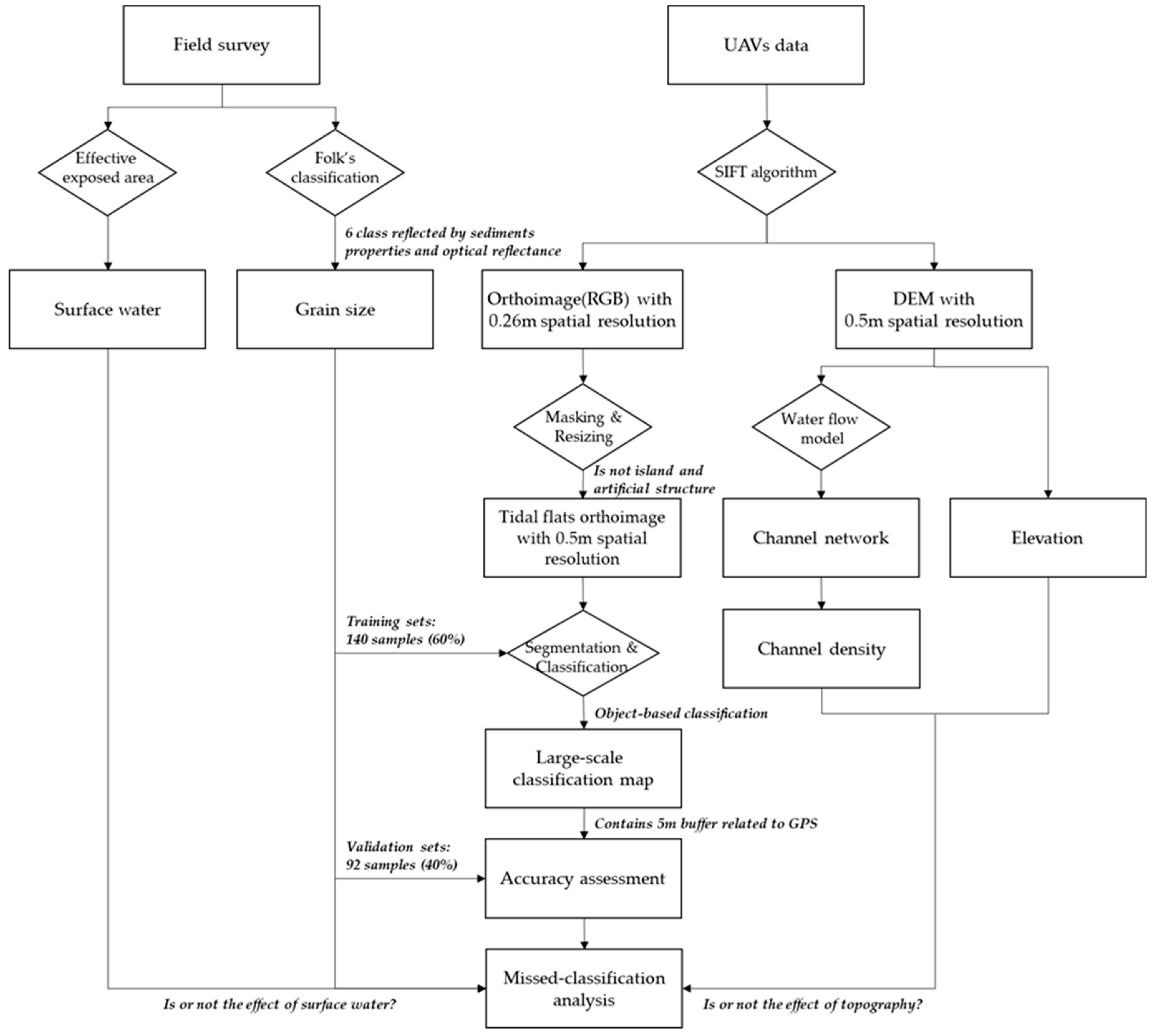
3.3. Surface Sediment Classification Procedure

The surface sediment classification procedure uses an object-based classification approach and the spectral characteristics of each pixel, such as texture, shape, and spatial relationships [20]. It was performed using Definiens^R Developer 9.1, a commercial image analysis software package developed by Definiens Imaging Co., particularly for use with high-resolution imagery [21]. Desclee et al. [22] and Conchedda et al. [23] provided details of the object-based method. We used the UAV-acquired RGB orthoimages for surface sediment classification in the study area during the segmentation process, in view of its strong sensitivity to soil and water content according to the elevation, tidal channel, and sediment type. The study area included tidal flats, islands, and roads. We masked the islands and roads to optimize the classification accuracy during image preprocessing. First, we performed image segmentation based on a multi-resolution segmentation algorithm. Multi-resolution segmentation makes objects using an iterative algorithm. The objects are determined by setting scale, shape, and compactness parameters [24]. The parameter weights are established according to their empirical values, to identify weights that are clearly distinct among the classification items. The segmentation process was performed with a focus on determining the weights dividing each tidal channel boundary and color, to distinguish the surface sediment by the shape and density of the tidal channel and mud content [4,25]. We performed a scale parameter, divided into five steps based on the spatial resolution of the image data. Scale 50 and 40 showed no boundaries. However, scale 30 revealed the boundaries of the tidal channels. Scales 20 and 10 distinguished more than the tidal channel boundaries. We established scale 30, shape 0.1, and compactness 0.5. The following process was then used to assign the objects to six classes derived from Folk’s classification. This will be discussed in Section 4.1. The training set randomly comprised 60% of all samples of each class; the other samples were used for accuracy assessment. The following process for classification of surface sediments adopted a hierarchical classification algorithm [24]. This algorithm estimated the membership value of an image object against a list of selected classes. The classification result of the objects were updated according to the class evaluation. The three best classes were stored as image object classification result. Classes without a class description were assumed to have a membership value of 0. Class related to features was considered only if enabled by the according parameter. Finally, to assess the accuracy of the sediment classifications, we determined the users and producers, and calculated the overall accuracy and kappa coefficient. We additionally analyzed the misclassified samples using the DEM, tidal channel density, grain size, and surface water. Figure 3 illustrates the procedure of surface sediment classification.

4. Results and Discussion

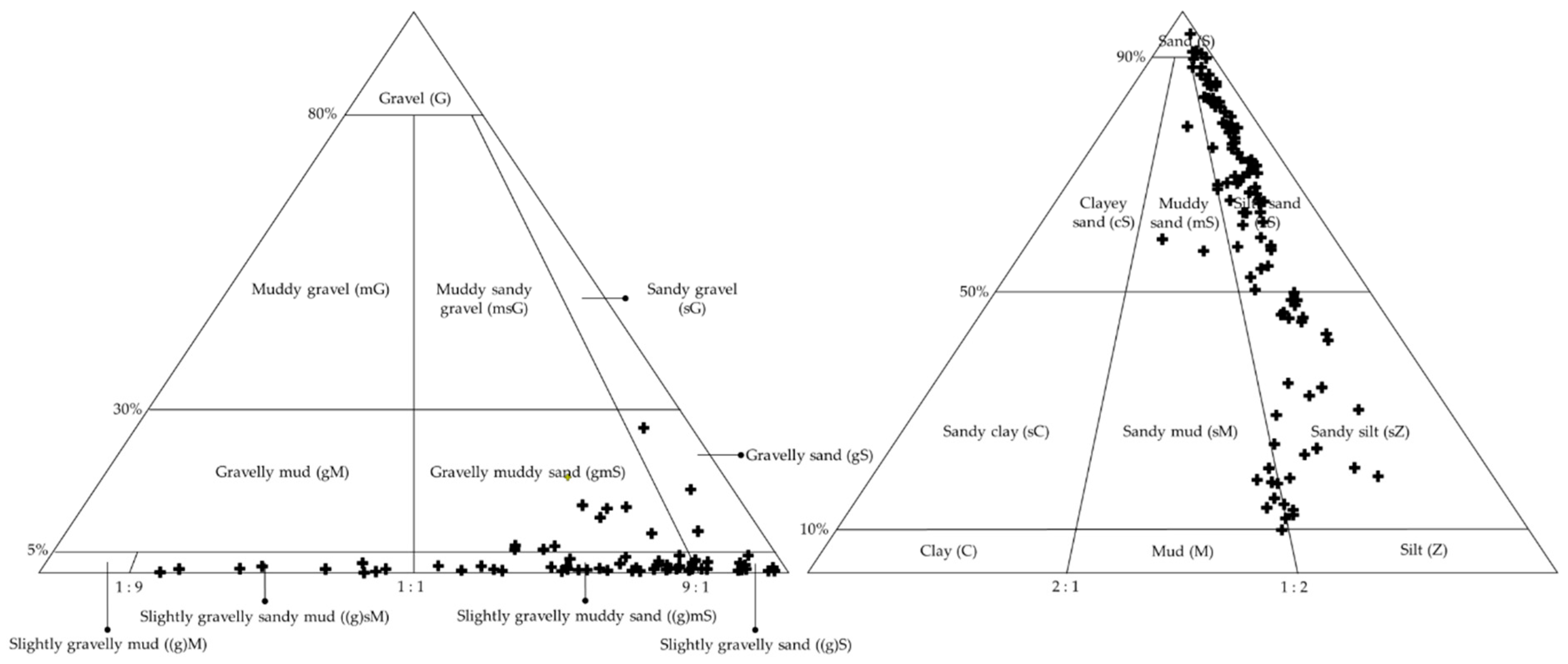
4.1. Analysis of Grain Size Distribution

We analyzed the surface sediment to determine the grain size criteria according to the spatial resolution of the UAV orthoimage. First, we analyzed the grain size distribution using by SEDCLASS and SEDPLOT program based on Folk’s classification. These programs were provided by Coastal and Marine Geology, U.S. Geological Survey (USGS). The surface sediment on the tidal flat variously consists of sand and mud. Folk’s triangle diagram indicated that the sediment consisted of 10 types: gravelly sand (gS), slightly gravelly sand ((g)S), sand (S), gravelly muddy sand (gmS), slightly gravelly muddy sand ((g)mS), silty sand (zS), muddy sand (mS), sandy silt (sZ), slightly gravelly sandy mud ((g)sM), and sandy mud (sM). Seventy percent of the study area consisted of zS, mS, gmS, and (g)mS, while gsM, (g)sM, and sZ were widely distributed across the tidal flat. The remaining sediment types had distributions of less than 10% (Figure 4).

Choi et al. (2010) and Ryu et al. (2003) described that critical grain size and water content are important factors for surface sediment classification based on remotely sensed data. Therefore, six classes were determined by mean, sorting, and mud content obtained by a field survey (

Table 2. Classification of sediment types based on sediment properties in accordance with Folk’s classification.

Class	Sediment Type by Folk (1986)		Composition (%)				Statistical Parameters
			Gravel	Sand	Silt	Clay	Mean (ø)	Sorting (ø)	Skewness	Kurtosis
1	gS	Average	17.6	76.9	3.4	2.0	0.8	2.0	−0.1	1.2
		Range	8.7~27.0	67.8~84.1	1.9~4.9	1.9~2.3	0.4~1.6	1.8~2.2	−0.3~0.1	1.0~1.4
	(g)S	Average	0.9	93.9	3.2	2.0	2.0	1.1	0.0	1.6
		Range	0.1~3.3	89.6~98.0	3.3~7.1	1.6~3.6	0.8~2.6	0.4~1.7	−0.2~0.3	1.0~2.9
2	S	Average	0.0	92.1	5.5	2.5	2.8	0.9	0.3	1.8
		Range	0.0~0.0	90.8~95.1	3.3~7.1	1.6~3.6	2.4~3.4	0.6~1.2	0.1~0.4	1.2~2.8
3	gmS	Average	9.2	71.4	13.1	6.2	2.6	2.6	0.0	2.0
		Range	5.2~15.8	61.7~79.8	8.3~23.2	3.8~11.0	2.0~3.8	2.2~3.0	−0.2~0.4	1.3~2.7
	(g)mS	Average	0.8	77.0	16.3	5.9	3.4	1.7	0.4	1.9
		Range	0.0~4.9	52.6~89.1	6.1~33.3	1.8~19.0	1.9~5.0	0.8~3.0	0.0~0.7	0.9~3.2
4	zS	Average	0.0	72.3	21.6	6.1	3.8	1.6	0.5	1.8
		Range	0.0~0.0	50.9~89.1	7.8~39.9	2.3~14.4	2.9~5.5	0.9~2.5	0.2~0.7	1.2~3.2
	mS	Average	0.0	70.9	16.5	12.6	4.0	2.2	0.6	1.8
		Range	0.0~0.0	56.7~89.2	6.5~23.9	4.3~24.0	2.4~5.5	1.4~2.9	0.3~0.8	0.8~2.8
5	sZ	Average	0.0	34.7	48.9	16.4	5.4	2.3	0.5	1.2
		Range	0.0~0.0	13.2~49.3	38.3~63.9	9.7~28.4	4.6~6.8	1.9~2.8	0.3~0.7	0.9~1.6
6	(g)sM	Average	0.4	28.3	48.6	22.7	6.0	2.7	0.3	1.0
		Range	0.1~1.3	12.6~46.4	34.5~62.4	12.2~31.4	4.8~6.8	2.2~3.3	0.2~0.5	0.8~1.4
	sM	Average	0.0	16.8	53.6	29.7	6.7	2.8	0.3	0.9
		Range	0.0~0.0	10.7~21.8	49.4~58.1	28.0~31.8	6.4~7.0	2.6~2.9	0.2~0.4	0.8~1.0

). Class 1 consists of gS and (g)S, and the gravel, sand, silt, and clay contents were 0.9–17.6%, 76.9–93.9%, 3.2–3.4%, and 2.0%, respectively. Class 2 was composed of S sediments without gravel content. The contents of sand, silt, and clay were 90.8–95.1%, 3.3–7.1%, and 1.6–3.6%, respectively. Classes 1 and 2 have very low mud content (< 8%). In addition, the mean and sorting values are 0.8–2.8Ø and less than 2Ø, respectively. It appears that the soil permeability is high, but the skewness is less than 0.3. This indicates that these classes are primarily associated with lower tidal energy; they are also affected by seawater related to tidal current. Class 3 is composed of gmS and (g)mS. Its gravel, sand, silt, and clay contents were 0.8–9.2%, 71.4–77%, 13.1–16.3%, and 5.9–6.2%, respectively. Class 4 is composed of zS and mS. Its sand, silt, and clay were 70.9–72.3%, 16.5–21.6%, and 6.1–12.6%, respectively. As mentioned previously, classes 3 and 4 are the most widely distributed across the study area. Their sediment compositions are similar; however, class 4 has no gravel content, and its mud content is 8% higher than that of class 3. The area is mostly composed of muddy sediments (3Ø or more), and the skewness exceeds 0.4. Class 4 is likely to be distributed in a place where the tidal energy is higher than that of class 3. Class 5 comprises sZ without gravel content, and with sand, silt, and clay contents of 34.9%, 48.9%, and 16.4%, respectively. Class 6 includes (g)sM and sM. Its gravel, sand, silt, and clay contents were 0.0–0.4%, 16.8–28.3%, 48.6–53.6%, and 22.7–29.7%, respectively. Classes 5 and 6 have mud contents that are greater than 65% and sand contents under 35%. This indicates that their mud content is significantly higher, while their sand content is significantly lower, than those of other classes. The mean exceeds 5Ø, the sorting is very poor, and the skewness is 0.3 to 0.5. These classes are likely to be distributed in areas with similar tidal currents to those associated with class 4.

The relationship between optical reflectance and sediment properties corresponds to the well-documented relationship with grain characteristics [3,8]. The distribution of surface sediment across a tidal flat is closely related to the tidal topography. The tidal channel is the key factor influencing the water content of sediment, while the topography is key in determining the exposure duration. The classification of surface sediment using remotely sensed data should consider topographic characteristics, such as ridge-runnel structure and ripple marks [2,26,27]. Figure 5 illustrates the correlation between sediment composition and factors of the depositional environment at line Y2 (32 samples). Figure 5a is the UAV RGB orthoimage; it shows the tidal channel network in relation to sediment distribution. Figure 5b shows the distribution of exposure duration estimated on the basis of tide height over 1 year, and the UAV DEM; it is divided into zones I, II, and III. Figure 5c–f shows the sediment composition distribution, topographic altitude change, tidal channel density, and surface water, respectively. The mud flat with less than 30% sand content was composed of (g)sM, sM, and sZ, and had densely distributed (more than 0.05 m/m²) dendritic and meandering dendritic channels. This area is located in the upper region of the tidal flat (> 0.38 m) with its exposure duration ranging between 12 and 24 hours (zone III). There is rarely any surface water. The mixed flat where the sand content exceeded 30% was composed of zS and mS. It has linear and linear dendritic channels with distributions of less than 0.05 m/m². This area is located at an altitude of -0.92 to 0.38 m, its exposure duration ranging between 6 and 12 hours (zone II). The surface water has dramatically increased by more than 10%. The sand flat, which constituted more than 70%, is composed of gmS, (g)mS, S, gS, and (g)S. This region contains linear tidal channels, with very low tidal channel density (< 0.05 or 0.02 m/m²). It is located in the lower area of the tidal flat (< −0.92 m) with an exposure duration of under 6 hours (zone I). The surface water exceeded 20%.

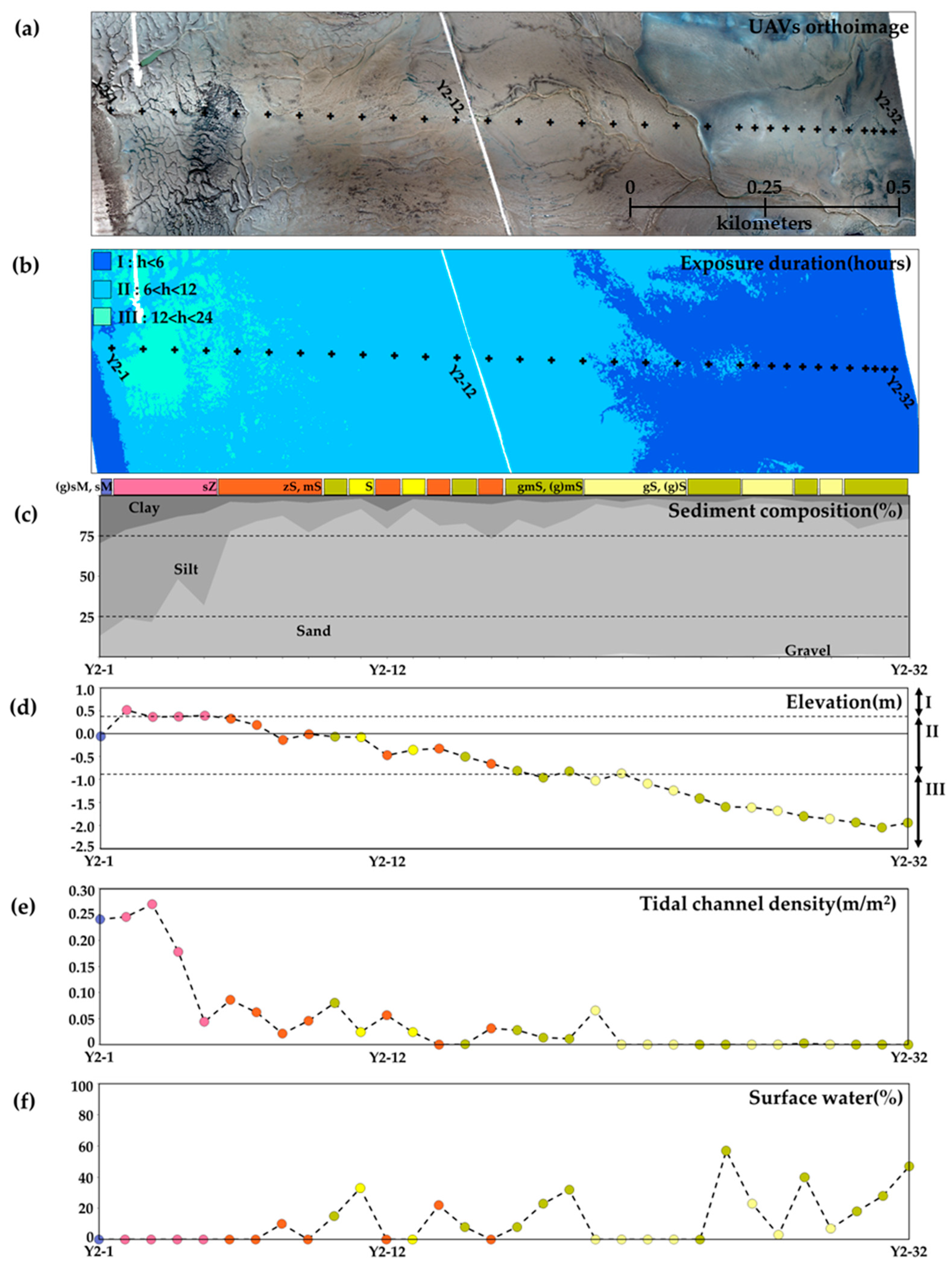
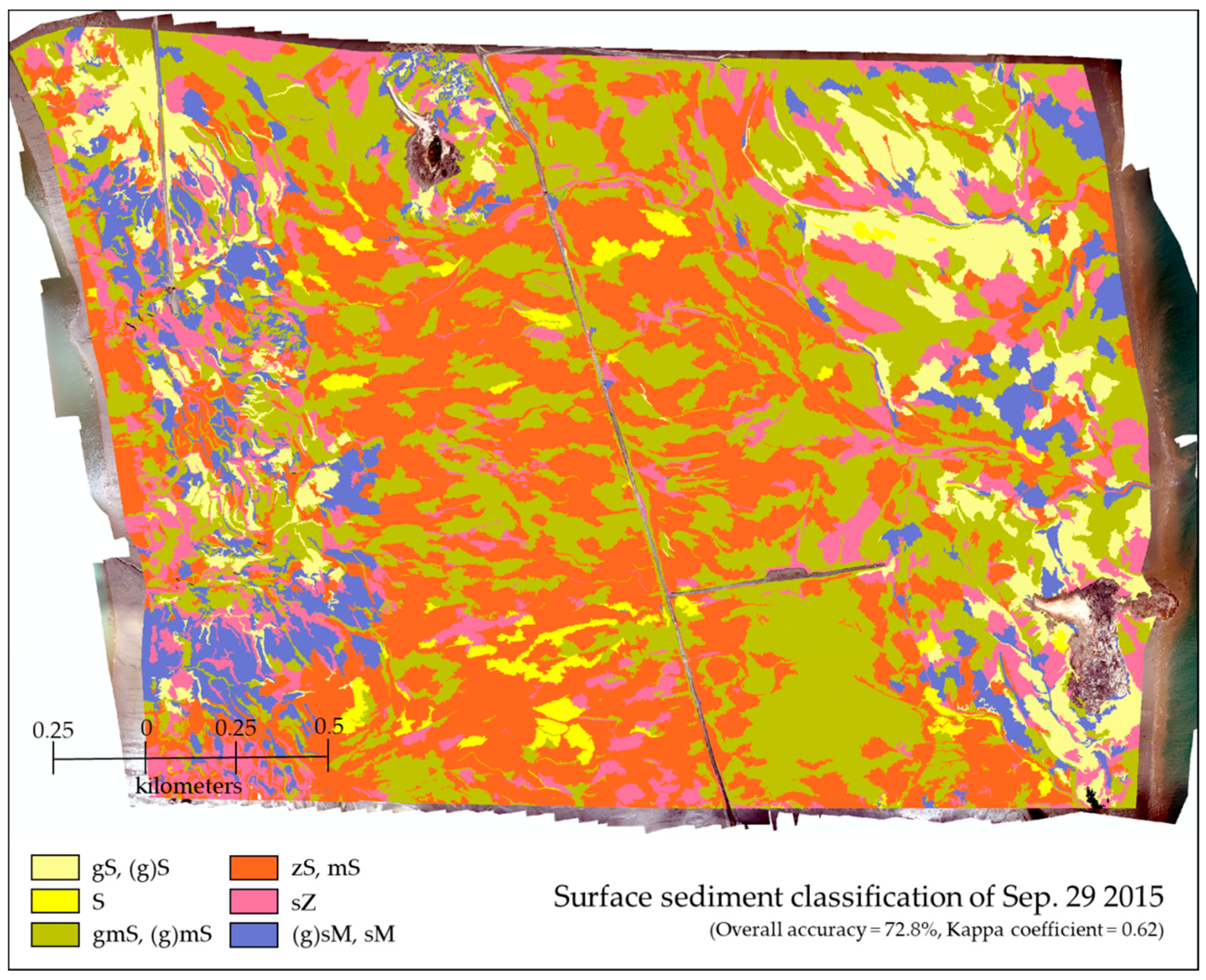
4.2. Surface Sediment Classification

Figure 6 presents a large-scale map of surface sediment classification generated using the object-based method.

Table 3. Accuracy assessment of the surface sediment classification. The overall accuracy is 72.83%, and the Kappa coefficient is 0.62.

Class		Classification of UAV Orthoimagery						Total Points	User Accuracy
		1	2	3	4	5	6
Reference data (in situ measurement)	1	5	0	1	0	0	1	7	0.71
	2	0	1	0	2	0	0	3	0.33
	3	1	1	23	3	1	2	31	0.74
	4	0	0	4	29	1	0	34	0.85
	5	0	0	1	2	5	1	9	0.56
	6	0	0	1	1	2	4	8	0.50
Total points		6	2	30	37	9	8	92	-
Producer Accuracy		0.83	0.50	0.77	0.78	0.56	0.50	-	-
Overall accuracy						72.38
Kappa coefficient						0.62

presents the accuracy assessment results for the surface sediment classification. A total of 92 samples were used in this process, of which 25 were misclassified. The results of the accuracy assessment indicated that the overall accuracy and Kappa coefficient were 72.8% and 0.62, respectively, with a 5-m error range related to the GPS device.

Figure 7 described all of the misclassified samples and the corresponding in situ photographs. Circles are incorrectly classified by the sun-glint effect and cloud. Triangles are misclassified by shellfish beds. Other misclassified samples were caused by surface water.

Around 30% of the misclassified samples (i.e., seven samples) were located at the edges of the image, and the optical reflectance was high due to the sun-glint effect. The sun-glint caused by flight direction was perpendicular to a solar azimuth angle. Another cause of misclassification was the presence of cloud shadows. The mud content and elevation of the study area are lower to the east, where the Hwang-do tidal flat can be found. There are numerous shellfish beds, including oyster and clam. Around 15% of the misclassified samples (i.e., four samples) were located in shellfish beds. The shellfish beds were relatively dark in the orthoimage. It seems to affect the optical reflectance of the misclassified samples. Generally, the gravel and sand had higher optical reflectance values than the silt and clay [7]. Other misclassified samples (i.e., fourteen samples) were slightly different in mud content, of about 1–7%, compared to the samples that had been properly classified. Therefore, this difference exerted little influence on the spectral absorption pattern according to the proportions of sand and mud. As previously mentioned, the optical reflectance was affected by the water content [2,8,15,20]. Most tidal flats are saturated with seawater under tidal influences. Based on the tidal height data recorded at Boryeong tide station in 2013, the exposure duration was under 12 hours across 95% of the study site. This indicates that most sediments are saturated, and that the seawater is likely to be distributed across the study area [2]. Choi et al. [4] described the interplay between intertidal DEM, tidal channel, local curvature, and water content. These tidal topography parameters can affect the distribution of the water content, including surface and interstitial water. To assess the effects of water content on optical reflectance, we analyzed the correlations between surface water, elevation, tidal channel density, and sediment properties (Figure 8).

Figure 8a,b illustrates the correlation between the elevation and tidal channel density, according to the surface water. There was a negative correlation between the elevation and the surface water when the surface water was less than 40%. However, where the surface water exceeded 40%, it had a positive correlation with elevation. Additionally, where the surface water was less than 40%, the correlation between surface water and tidal channel density was negative, while the tidal channel density was lower when the surface water exceeded 40%. Figure 8c,d depicts the correlation between sediment properties and surface water. According to the results of our analysis, the mud content, mean, and sorting values showed a negative correlation with the surface water amount when the surface water was less than 40%. Where the surface water exceeded 40%, the mud content, mean, and sorting values showed a positive correlation with the surface water. In summary, the surface water increased as the elevation, tidal channel density, and the mud content, mean, and sorting values amount decreased, when the surface water was less than 40%. By contrast, when the surface water exceeded 40%, the surface water increased as the elevation, the mud content, mean, and sorting values amount increased. The tidal channel density was low (< 0.02). It seems that the surface water increased as the surface permeability is poor. As a result of analyzing 14 misclassified samples, most samples were located in lower area (< -0.4 m) and lower tidal channel density (< 0.05 m/m²). They may be covered in surface water, and the surface water would have affected the optical reflectance. The samples were mostly classified to the class of higher mud content. However, some of the samples were classified to the class of lower mud content. It seems that the optical reflectance increased in response to the addition of seawater to fully saturated sediments [28]. Other samples were distributed at higher area (> 0.2 m) and higher tidal channel density (> 0.2 m/m²). Those were classified to the class of higher mud content. The optical reflectance may be affected by water film in less than 5% water content [29].

5. Conclusions

We investigated the possibility of generating a large-scale surface sediment map using UAV data (combined with a field survey), including grain size, elevation, and water content at 232 sites on the Hwang-do tidal flat. The conclusions are as follows:

To determine the grain size criteria for the UAV data, we analyzed the sediment properties, such as grain composition, and statistical variables obtained by a field survey conducted at the 232 sites. We divided the sediment into six types according to the mud content, mean, and sorting. Classes 1 and 2 have very low mud contents, of less than 8%; their mean and sorting values are 0.8–2.8Ø and less than 2Ø, respectively. This indicated that the permeability is high, and that these classes are mostly distributed in areas with lower tidal energy, partly due to the seawater and tidal current. Classes 3 and 4 are predominant in the study area. Their sediment compositions are similar; however, class 4 has no gravel content and its mud content is 8% higher than that of class 3. The mean is 3Ø or greater, due to it being comprised mainly of muddy sediments, and the skewness was greater than 0.4. Class 4 is likely to be distributed in a location where the tidal energy is higher than that of class 3. Classes 5 and 6 have mud contents in excess of 65% and sand contents of less than 35%; i.e., the mud content is significantly higher, and the sand content significantly lower, than those of the other classes. The mean is greater than 5Ø and the sorting is very poor, and the skewness is 0.3 to 0.5. These classes are likely to be distributed in areas with similar tidal currents to those of class 4.

The UAV RGB orthoimage was used in combination with field survey data to produce a map of the surface sediment classification via an object-based method. An overall accuracy of 72.8% was achieved. Seven misclassified samples were affected by sun glint and cloud shadows. The effect of sun glint would be improved by overlapping many images. Rotary-wing UAVs have difficulty acquiring sufficient images to reduce the effect of sun-glint limited with regard to observation time. A fixed-wing UAV or vertical take-off and landing (VTOL) aircraft may obtain sufficient images over a longer period, allowing the effects of sun glint to be minimized by increasing the overlap range between the images. Additionally, we consider that UAV observation would be conducted to reduce the effects of sun glint on a cloudy day. Four misclassified samples were located in shellfish beds. The shellfish beds were effectively detected via the texture features method, using Terra SAR-X data [13]. This implies that integration of the optic and radar data could improve the accuracy of surface sediment classification by distinguishing the shellfish beds from the tidal flat.

The Hwang-do tidal flat is typically exposed for less than 12 hours. It has high moisture content. This environmental condition is an important factor affecting the optical reflectance. We analyzed the 14 misclassified samples by investigating the correlations among elevation, tidal channel density, and sediment properties according to the surface water. The misclassified samples had relatively higher surface water or lower surface water according to topographic features. The surface water may influence the optical reflectance. Rainy et al. (2000) [6] showed that the surface water has low optical reflectance at longer wavelengths (>700 nm). To improve the accuracy of the surface sediment classification, additional NIR band and SWIR band are needed, and a thematic map of the surface water should be generated. If the thematic map is used as input data in the classification procedure or mask file for eliminating areas of water coverage in the image preprocessing, the accuracy may be improved.

In summary, our research indicates that highly accurate, large-scale classification of surface sediment is possible using UAV data. However, regarding the acquisition of high-quality maps of surface sediment classification, limitations remain with respect to the observation system and the effect of surface water and shellfish beds. Additional multi-spectral information and integration of radar data could be possible to improve the surface sediment classification. The result is specific to the characteristics of surface sediment on the Hwang-do tidal flat. To enhance understanding of the detailed surface sediment distribution on tidal flats, further work on different areas will be necessary.

References

1. Marani, M.; D’Alpaos, A.; Lanzoni, S.; Carniello, L.; Rinaldo, A. Biologically-controlled multiple equilibria of tidal landforms and the fate of the Venice lagoon. Geophys. Res. Lett. 2007, 34, L11402. [Google Scholar] [CrossRef]
2. Ryu, J.H.; Na, Y.H.; Won, J.S.; Doerffer, R. A critical grain size for Landsat ETM+ investigations into intertidal sediments: A case study of the Gomso tidal flats, Korea. Estuar. Coast. Shelf Sci. 2004, 60, 491–502. [Google Scholar] [CrossRef]
3. Rainey, M.P.; Tyler, A.N.; Bryant, R.G.; Gilvear, D.J.; McDonald, P. The influence of surface and interstitial moisture on the spectral characteristics of intertidal sediment: Implications for airborne image acquisition and processing. Int. J. Remote Sens. 2000, 21, 3025–3038. [Google Scholar] [CrossRef]
4. Choi, J.K.; Eom, J.; Ryu, J.H. Spatial relationship between surface sedimentary facies distribution and topography using remotely sensed data: Example from the Ganghwa tidal flat, Korea. Mar. Geol. 2011, 280, 205–211. [Google Scholar] [CrossRef]
5. Doerffer, R.; Murphy, D. Factor analysis and classification of remotely sensed data for monitoring tidal flats. Helgol. Meeresunters. 1989, 43, 275–293. [Google Scholar] [CrossRef] [Green Version]
6. Rainey, M.P.; Tyler, A.N.; Givear, D.J.; Bryant, R.G.; McDonald, P. Mapping intertidal estuarine sediment grain size distributions through airborne remote sensing. Remote Sens. Environ. 2003, 86, 480–490. [Google Scholar] [CrossRef]
7. Jensen, J.R. Remote Sensing of the Environment, 3rd ed.; Prentice Hall: Upper Saddle River, NJ, USA, 2000; ISBN 978-0131889507. [Google Scholar]
8. Ryu, J.H.; Choi, J.K.; Na, Y.H.; Won, J.S. Characteristics of Landsat ETM+ image for Gomso Bay tidal flat sediments Korean. J. Remote Sens. 2003, 19, 117–133. [Google Scholar]
9. Bartholdy, J.; Folving, S. Sediment classification and surface type mapping in the Danish Wadden sea by remote-sensing. Neth. J. Sea Res. 1986, 20, 337–345. [Google Scholar] [CrossRef]
10. Yates, M.G.; Jones, A.R.; McGrorty, S.; Goss-Custard, J.D. The use of satellite imagery to determine the distribution of intertidal surface sediments of the Wash, England. Estuar. Coast. Shelf Sci. 1993, 36, 333–344. [Google Scholar] [CrossRef]
11. Choi, J.K.; Ryu, J.H.; Lee, Y.K.; Yoo, H.R.; Woo, H.J.; Kim, C.H. Quantitative estimation of intertidal sediment characteristics using remote sensing and GIS. Estuar. Coast. Shelf Sci. 2010, 88, 125–134. [Google Scholar]
12. Eom, J.; Choi, J.K.; Lee, Y.K.; Ryu, J.H.; Won, J.S. Standardization of sedimentary facies and topography based on the tidal channel type in Western coastal area, Korea. J. Coast. Res. 2013, 65, 1373–1378. [Google Scholar] [CrossRef]
13. Jung, R.; Adolph, W.; Ehlers, M.; Farke, H. A multi-sensor approach for detecting the different land covers of tidal flats in the German Wadden Sea-a case study at Norderney. Remote Sens. Environ. 2015, 170, 188–202. [Google Scholar] [CrossRef]
14. Adolph, W.; Farke, H.; Lehner, S.; Ehlers, M. Remote Sensing Intertidal Flats with TerraSAR-X. A SAR Perspective of the Structural Elements of a Tidal Basin for Monitoring the Wadden Sea. Remote Sens. 2018, 10, 1085. [Google Scholar] [CrossRef]
15. So, J.G.; Jeong, G.T.; Chae, J.W. Numerical Modeling of Changes in Tides and Tidal Currents Caused by Embankment at Chonsu Bay. JKSCOE 1998, 10, 151–164. [Google Scholar]
16. Kim, Y.S.; Kim, J.N. Biogenic sedimentary structures of crustaceans at the intertidal flat of Whang Island, Cheonsu Bay (Korean edn.). JKESS 1996, 17, 357–364. [Google Scholar]
17. Lee, J.H.; Park, H.S. Community structures of macrobenthos in Chonsu bay, Korea. J. Korea Soc. Oceanogr. 1998, 33, 18–27. [Google Scholar]
18. Folk, R.L. A review of grain size parameters. Sedimentology 1968, 6, 73–93. [Google Scholar] [CrossRef]
19. Eom, J. Fractal Analysis of Inter-Tidal Channels and Creeks Using High Resolution Satellite Images Korea; Yonsei University: Seoul, Korea, 2008. [Google Scholar]
20. Blaschke, T.; Strobl, J. What’s wrong with pixels? Some recent development interfacing remote sensing and GIS. Interfac. Remote Sens. GIS 2001, 6, 12–17. [Google Scholar]
21. Walsh, S.J.; McCleary, A.L.; Mena, C.F.; Shao, Y.; Tuttle, J.P.; Gonzalez, A.; Atkinson, R. QuickBird and Hyperion data analysis of an invasive plant species in the Galapagos Islands of Ecuador: Implications for control and land use management. Remote Sens. Environ. 2008, 112, 1927–1941. [Google Scholar] [CrossRef]
22. Desclee, B.; Bogaert, P.; Defourny, P. Forest change detection by statistical object-based method. Remote Sens. Environ. 2006, 102, 1–11. [Google Scholar] [CrossRef]
23. Conchedda, G.; Durieux, L.; Mayaux, P. An object-based method for mapping and change analysis in mangrove ecosystems. ISPRS J. Photogramm. Remote Sens. 2008, 63, 578–589. [Google Scholar] [CrossRef]
24. Trimble. eCognition® Developer 9.0 Reference Book; Trimble Germany GmbH: Munich, Germany, 2014. [Google Scholar]
25. Eom, J.; Choi, J.K.; Ryu, J.H.; Woo, H.J.; Won, J.S.; Jang, S. Tidal channel distribution in relation to surface sedimentary facies based on remotely sensed data. Geosci. J. 2012, 16, 127–137. [Google Scholar] [CrossRef]
26. Jang, S.; Han, H.; Lee, H. Observation of ridge-runnel and ripples in Mongsanpo intertidal flat by satellite SAR imagery. Korean J. Remote Sens. 2010, 26, 115–122. [Google Scholar]
27. Van der Wal, D.; Herman, P.M.J.; Wielemaker-van den Dool, A. Characteristics of surface roughness and sediment texture of intertidal flats using ERS SAR imagery. Remote Sens. Environ. 2005, 98, 96–109. [Google Scholar] [CrossRef]
28. Liu, W.; Baret, F.; Gu, X.; Tong, Q.; Zheng, L.; Zhang, B. Relating soil surface moisture to reflectance. Remote Sens. Environ. 2002, 81, 238–246. [Google Scholar]
29. Neema, D.L.; Shah, A.; Patel, N. A statistical optical model for light reflection and penetration through sand. Int. J. Remote Sens. 1987, 8, 1209–1217. [Google Scholar] [CrossRef]
Figure 1. Kompsat-3 panchromatic image of the Cheonsu bay and Hwang-do tidal flat, acquired on March 23, 2015. (a) The square-dotted line delineates the study area (Site A), which is the unmanned aerial vehicle (UAV) survey site. The area is around 2.5 km2 in size. The crosses and yellow boxes indicate the measurement sites for grain size, elevation, and surface water on September 29–30, 2015. The red and green circles are the measurement sites for grain size and elevation from 2004 to 2013. (b,c) show the sediment composition in May 2010 and May 2013 at the H sites. (d) Shows the change in elevation between May 2010 and June 2013. Erosion and sedimentation of sediment at the C sites can be seen.
Remotesensing 11 00229 g001
Figure 2. Flight paths of UAV. The squares are image footprints, which had 70% side-lap and a 60% forward-lap. The crosses are GCP.
Remotesensing 11 00229 g002
Figure 3. Large-scale classification of surface sediment distribution using an UAV orthoimage (red, green, blue; RGB) combined with a field survey conducted at 232 sites. To map the large-scale sediment distribution, 140 and 92 samples were used as training and validation sets, respectively. The field survey produced the grain size, elevation, and surface water data, which were used to analyze the missed classification samples.
Remotesensing 11 00229 g003
Figure 4. Analysis of grain size using the 232 samples acquired from a field survey, based on Folk’s classification. This diagram shows that sediments consist of gravelly sand (gS), slightly gravelly sand ((g)S, sand (S), gravelly muddy sand (gmS), slightly gravelly muddy sand ((g)mS), silty sand (zS), muddy sand (mS), sandy silt (sZ), slightly gravelly sandy mud ((g)sM), and sandy mud (sM).
Remotesensing 11 00229 g004
Figure 5. Correlation between sediment composition and depositional environment factors at line Y2. (a,b) show the tidal channel network and exposure duration extracted from UAV and tide height data; (c) indicates that the sediment type is related to the sediment composition, which controls the elevation, tidal channel density, and surface water (d, e, and f, respectively).
Remotesensing 11 00229 g005
Figure 6. Large-scale surface sediment classification map derived from the UAV RGB orthoimage. The overall accuracy is 72.8%, with a 5-m error range, and the Kappa coefficient is 0.62.
Remotesensing 11 00229 g006
Figure 7. Overview of misclassified samples on tidal flat of Hwang-do, imaged by UAV orthoimage and the corresponding in situ photographs. The circles are affected by sun-glint and cloud. The triangles are misclassified samples due to shellfish beds. The crosses indicate that the misclassified samples are affected by surface water.
Remotesensing 11 00229 g007
Figure 8. Correlations among topography, sediment properties according to the surface water; (a,b) indicate the relationships among elevation, tidal channels, and surface water, and (c,d) indicate the relationships among mud content, mean and sorting values, and surface water. The error bar is the standard error, which is the standard deviation of each category divided by the number of samples (Error bar = standard deviation/√number of samples).
Remotesensing 11 00229 g008