Temporal Transferability of Pine Forest Attributes Modeling Using Low-Density Airborne Laser Scanning Data

Abstract

This study assesses model temporal transferability using airborne laser scanning (ALS) data acquired over two different dates. Seven forest attributes (i.e. stand density, basal area, squared mean diameter, dominant diameter, tree dominant height, timber volume, and total tree biomass) were estimated using an area-based approach in Mediterranean Aleppo pine forests. Low-density ALS data were acquired in 2011 and 2016 while 147 forest inventory plots were measured in 2013, 2014, and 2016. Single-tree growth models were used to generate concomitant field data for 2011 and 2016. A comparison of five selection techniques and five regression methods were performed to regress field observations against ALS metrics. The selection of the best regression models fitted for each stand attribute, and separately for both 2011 and 2016, was performed following an indirect approach. Model performance and temporal transferability were analyzed by extrapolating the best fitted models from 2011 to 2016 and inversely from 2016 to 2011 using the direct approach. Non-parametric support vector machine with radial kernel was the best regression method with average relative % root mean square error differences of 2.13% for 2011 models and 1.58% for 2016 ones.

1. Introduction

Forest ecosystems provide economic and social benefits to humankind [1,2] requiring accurate tools to monitor their dynamics over time [3]. Over the last decades, optical remote sensing techniques have been used for monitoring forest changes at regional scales with the support of field surveys (e.g., [4,5]). However, airborne laser scanning (ALS) is better adapted to characterize forest structure [6] and estimate forest inventory parameters, providing accurate information to perform forest management and planning [3]. Furthermore, costs of ALS-based inventories are comparable to those associated with traditional ground-based ones [7,8]. Despite the great potential of this technology, multi-temporal ALS data have been utilized less, as the availability of two or more surveys in the same area has been limited by acquisition costs as well as by the need of temporal-concomitant field data (e.g., [3,6,9,10]). Recently, organizations, companies, and countries have made an effort to gather multi-temporal datasets in different years (e.g., [11,12,13]) allowing the estimation of biophysical properties in forested areas over time. As a result, height growth has been estimated using the single tree or the area-based approach [14,15,16,17,18,19,20]. Biomass and carbon dynamics has also been analyzed [3,9,21,22,23,24,25,26,27], while less studies have estimated volume [17,18,21], basal area [17], and site index [14,28]. Multi-temporal data has also been used for quantifying fire-induced changes to forest structure [29], gaps presence [20,30,31] or detecting defoliation [32]. However, to the best of our knowledge, some relevant forest inventory attributes, such as stand density, squared mean diameter, and dominant diameter, have not been estimated using multi-temporal ALS data.

The use of low-density ALS data has been successfully used for estimating forestry attributes in different forest ecosystems (e.g., [33,34,35]), being also the case in Mediterranean forests of Spain (e.g., [36,37,38]). The analysis of the influence of point density on model predictions have been analyzed by several authors (e.g., [39,40,41]), who established that point density has little or no effect on predictions as statistical metrics remain stable [42]. Furthermore, Garcia et al. [43], Singh et al. [44], and Ruiz et al. [45] pointed out that low-density datasets were a viable solution at regional scales. Furthermore, the use of multi-temporal, low-point density data has only been explored in boreal ecosystems [17,28] and in temperate forests [24,27] but not in other ecosystems, such as Mediterranean ones, which are characterized by a higher heterogeneity in terms of forest structure.

Direct and indirect approaches have been proposed to model forest attributes using multi-temporal ALS data over time [26]. The direct approach adjusts one model for one point in time and estimates the inventory attribute for another point in time [3,9]. Previously, the model to be extrapolated was generated through regression methods that related a suite of ALS-metrics with ground-truth data. This approach allowed the temporal transferability of models reducing modeling time and fieldwork, as it was not needed to revisit them when the time between the ALS surveys was not large [28]. In contrast, the indirect approach fits two different models and estimates the variables for each point in time [3,9,17,24,25,27]. Several examples of the evaluation of these two approaches can be found in the literature. For example, when estimating biomass and carbon fluxes, Zhao et al. [3] and Meyer et al. [25] achieved better results with the indirect approach while Cao et al. [9], Skowronski et al. [24], and Bollandsås et al. [26] found slightly better performance of the direct approach.

These aforementioned modeling strategies sometimes face a challenge when lacking temporally-concomitant field data to calibrate forest stand models [3]. To this end, forest growth models can serve as useful tools to calibrate forest stand variables in a specific point in time. Thus, empirical growth models have received particular attention since the beginning due to their usefulness. Nowadays state-space stand-level models [46], distribution-based models, and both individual-tree models and complex process-based eco-physiological models [47] have dramatically increased flexibility and realism to forest simulations. In this sense, individual-tree growth models are powerful tools to update stand variables to the Light Detection and Ranging (LiDAR) mission date. For example, the use of diameter at breast height (dbh) and the height growth values from general yield tables of the Spanish National Forest Inventory have been applied for estimating total tree biomass in Aleppo pine forests [36]. However, specific single-tree growth models calibrated with tree rings are more accurate, particularly for improving model consistency when working at regional scale.

Thus, the aim of this study is to assess temporal transferability of several forest attributes models by comparing direct and indirect approaches using low-density ALS datasets collected in 2011 and 2016. Seven forestry attributes (i.e. stand density, basal area, squared mean diameter, dominant diameter, tree dominant height, timber volume, and total tree biomass) are estimated at regional scale in the Mediterranean Aleppo pine forest. First, an indirect approach fits two different models for 2011 and 2016 and estimates stand attributes for each point in time using different ALS-metrics and model parameters. Secondly, a direct approach extrapolates the models fitted previously, using the same variables and model parameters, to the other points in time.

Furthermore, the following secondary objectives were addressed: updating field inventory data collected in three different dates to the point clouds acquisition dates using single-tree growth models; comparing five selection methods and five regression methods in forest attributes modeling.

2. Materials and Methods

2.1. Study Area

The Aleppo pine (Pinus halepensis Mill.) forests under study are located in the Aragón region (Figure 1), Northeast Spain. This species represents 18.7% of the forested area, including semi-natural and reforested stands [48] and is well adapted to Mediterranean environmental conditions.

In this area, the annual precipitation ranges from 350 mm to 1000 mm [49]. The average annual temperature is 14 °C, with cold winters and hot and dry summers. Aleppo pine forests are characterized by a hilly topography, with elevations ranging from 300 to 1150 m above sea level and slopes from 0° to 39°. The lithology of the study area varies from Miocene carbonate and marl sediments to limestone platforms and Mesozoic and Eocene limestone.

Some pine stands are natural, but most stands were planted approximately forty to sixty years ago. The evergreen understory includes species such as Quercus ilex subsp. rotundifolia, Quercus coccifera, Juniperus oxycedrus, Buxus sempervirens, Juniperus phoenicea, Rosmarinus officinalis, and Thymus vulgaris, among many others. Reforested areas usually present a low presence of hardwood species and poor diversity [50,51], while natural stands are structurally complex with a developed and diverse understory [52].

2.2. Forest Inventory Data

Forest inventory data was acquired through 147 plots from three field campaigns performed during June to July 2013, July to September 2014, and April 2016 (Figure 1), from now on cited as first, second, and third campaign, respectively. The sampling data fulfilled the statistical requirements [53], considered the size of the study area, and the variability of the pine forest in terms of terrain slope, canopy height, and canopy cover (CC) [54].

Field data from the first campaign were acquired in 53 circular plots with a 15 m radius. A Leica VIVA® GS15 CS10 GNSS real-time kinematic global positioning system (GPS) was used to collect the center of each plot. Tree dbh, for those trees with a dbh larger than 7.5 cm, was measured at 1.3 m height using a diameter tape. Green crown height and height of up to 4 randomly selected sample trees within each plot were measured using a Suunto® hypsometer. Thus, diametric class was considered when selecting the sample trees.

Field data from the second campaign were collected in 43 circular plots with a 15 m radius. The center of the plots was referenced using the same Global Navigation Satellite System (GNSS) receiver as in the first campaign. Tree dbh was measured with the same criteria as the first campaign using a Haglöf Sweden® Mantax Precision Blue caliper. The green crown height and the total height of all trees in the plot were measured using a Haglöf Sweden® Vertex instrument.

Field data from the third campaign were acquired in 51 circular plots. The center of the designated circular plots was measured using a Trimble® GNSS receiver. Field plots with a 5.6 m (3 plots), 8.5 m (23 plots), 11.3 m (17 plots), and 14.10 m (7 plots) radius were collected. Tree dbh was measured at 1.3 m using the same caliper as in the second campaign. The green crown height and the height of up to the 6 nearest trees to the plot center were measured using a Haglöf Sweden® Vertex instrument. The sample was completed to achieve 100 dominant stems ha⁻¹ considering those with larger dbh.

The height for those trees not measured in the field plots was predicted using a height–diameter model developed from the sampled trees from all the field plots of the third campaign. Normality of the residuals, homoscedasticity, and independence or no auto-correlation in the residuals were verified for the linear regression fitted model.

2.3. Inventories Updating and Stand Variable Computation

Field data measurements were updated to year 2011 and 2016, which correspond to each ALS flight, to avoid any temporal lag between ALS-metrics and stand-level variables. The PHRAGON-2017 individual tree model was applied [55] through the forest simulator platform Simanfor [56]. This model enables tree-level distance–independent simulation of the development of Aleppo pine afforestations in Aragón. It consists of a set of equations for diameter over bark growth, diameter under bark growth, diameter under bark–diameter over bark ratio, generalized height–diameter relationship, volume over bark (taper equation) and crown ratio. In addition, it presents a survival model for the coming 10-year period and a classification tree for the regeneration of species of the genus Pinus, Quercus, and Juniperus, also in the coming decade. Explanatory variables included those related to tree size (diameter at breast height, total height), stand density (basal area, Hart–Becking index), dominant trees (dominant height, dominant diameter), competition (BALMOD) [57] and site quality (site index). Site index and dominant height evolution were estimated using the site index curves developed for natural Aleppo pine forests in the central Ebro valley [58].

Thus, when projecting future stand variables, diameter growth and survival equations were applied to every single tree in each plot, while the site index curve was used to forecast the future stand dominant height (and hence estimate the total height of each surviving tree). To reconstruct stand structure in the past, we need to deploy the diameter under bark growth equation, as it permits the use of the current stand features to predict the past growth of a tree (backdating procedure). Therefore, past tree diameters over bark are estimated through the diameter under bark –diameter over bark ratio–, while past dominant height can be calculated with the same site index curves, as they are dynamic, age-independent functions. Once every diameter and dominant height are known, the rest of the stand variables can be directly computed.

Seven forest inventory attributes were calculated from field data for each plot: stand density (N); basal area (G); squared mean diameter (Dg); dominant diameter (Do); dominant height (Ho); timber volume over bark of stem (V); and total tree biomass (W) [37] (

Table 1. Forest inventory attributes.

Date of the Campaign	Field Data	Variables	Units
First: June to July 2013	Green crown height Total height Dbh	Stand density (N) Basal area (G) Squared mean diameter (Dg) Dominant diameter (Do) Dominant height (Ho) Volume over bark (V) Total tree biomass (W)	stems ha−1 m2 ha−1 cm cm m m3 ha−1 tons ha−1
Second: July to September 2014
Third: April 2016

). Thus, Ho is the mean height of the 100 trees per ha with largest dbh; Do is the mean dbh of the 100 trees per ha with largest dbh. V is estimated through the taper equation included in the PHRAGON-2017 individual-tree model [55]. W is computed as the sum of aboveground and belowground tree biomass using the Aleppo pine allometric equations developed by Ruiz-Peinado et al. [59].

2.4. ALS Data and Processing

The ALS data were acquired in 2011 and 2016 by the Spanish National Plan for Aerial Orthophotography (PNOA) [60]. The respective acquisition specifications are shown in

Table 2. Technical specifications of airborne laser scanning (ALS) data.

Characteristics	Year 2011	Year 2016
Time period	January to February	September to November
Laser scanning system	Leica ALS60	Leica ALS80
Wavelength	1,064 nm	1064 nm
Average flying altitude over sea level	3,000 m	3150 m
Pulse repetition frequency	~70 kHz	176–286 kHz
Scanning frequency	~45 kHz	28–59 Hz
Maximum scan angle	29°	25°
Nominal point density	0.5 points m−2	1 points m−2
Average point density	0.64 points m−2	1.25 points m−2
Accuracy of the point cloud (RMSEz)	≤0.2 m	0.09 m

. The point clouds, delivered in 2 × 2 km tiles in LAS binary file format, were captured with up to four returns measured per pulse. The x, y, and z coordinates were provided in European Terrestrial Reference System (ETRS) 1989 Universal Transverse Mercator (UTM) Zone 30 N.

After the noise removal from the point clouds, a verification of the overlapping returns was performed considering vertical and horizontal displacements. Thus, overlapping returns were removed from 105 tiles for the 2011 ALS flight. The subsequent steps were evenly applied for both ALS campaigns. The multiscale curvature classification algorithm [61], implemented in MCC 2.1 command line tool, was used to classify ground points according to Montealegre et al. [62]. A digital elevation model (DEM) with a 1-m size grid was generated using the Point-Triangulated Irregular Network-Raster interpolation method [61], implemented in ArcGIS 10.5 software. This DEM was used for point height normalization. The point clouds were clipped to the spatial extent of each field plot. Then, a full suite of statistical metrics related to height distribution and canopy cover was calculated [63] using FUSION LDV 3.60 [64] software. A threshold value of 2 m height was applied to remove ground and understory laser hits before generating the ALS-derived variables according to Nilsson [65] and Næsset and Økland [66]. For better understanding of the results, the ALS metrics were classified into three macro classes and seven classes (see

Table A1. Summary of the airborne laser scanning (ALS) computed metrics including the abbreviations, classes, and macro-classes defined.

Macro-Classes	Classes	ALS Computed Metrics	Abbreviations
Canopy height metrics (CHM)	Lower height variables	Minimum elevation	Elev. minimum
		01th percentile of the return heights	P01
		05th percentile of the return heights	P05
		10th percentile of the return heights	P10
		20th percentile of the return heights	P20
		25th percentile of the return heights	P25
		L moment 1 elevation	Elev. L1
		L moment 2 elevation	Elev. L2
	Mean height variables	Mean elevation	Elev. Mean
		Mode elevation	Elev. Mode
		30th percentile of the return heights	P30
		40th percentile of the return heights	P40
		50th percentile of the return heights	P50
		60th percentile of the return heights	P60
		70th percentile of the return heights	P70
		L moment 3 elevation	Elev. L3
		Elevation quadratic mean	Elev. SQRT mean SQ
		Elevation cubic mean	Elev. CUR mean CUBE
	Higher height variables	75th percentile of the return heights	P75
		80th percentile of the return heights	P80
		90th percentile of the return heights	P90
		95th percentile of the return heights	P95
		99th percentile of the return heights	P99
		Maximum elevation	Elev. maximum
		L moment 4 elevation	Elev. L4
Canopy height variability metrics (CHVM)	Variability	Standard deviation of point heights distribution	Elev. SD
		Variance of point heights distribution	Elev. Variance
		Coefficient of variation of point heights distribution	Elev. CV
		Skewness of point heights distribution	Elev. Skewness
		kurtosis of point heights distribution	Elev. Kurtosis
		Interquartile distance of point heights distribution	Elev. IQ
		Average Absolute Deviation of point heights distribution	Elev. AAD
	Variability L moment	L moment coefficient of variation of point heights distribution	Elev. LCV
		L moment skewness of point heights distribution	Elev. Lskewness
		L moment kurtosis of point heights distribution	Elev. Lkurtosis
Canopy density metrics (CDM)	% first, % all returns, canopy relief ratio	percentage of first returns above the 2.00	% first ret. above 2.00
		percentage of all returns above the 2.00	% all ret. above 2.00
		percentage of first returns above the mean	% first ret. above mean
		percentage of first returns above the mode	% first ret. above mode
		percentage of all returns above the mean	% all ret. above mean
		percentage of all returns above the mode	% all ret. above mode
		Canopy relief ratio	CRR
	All returns Total returns-1	All returns above 2.00 divided by the total first returns × 100	(All ret. above 2.00)/(total first ret.) × 100
		All returns above mean divided by the total first returns × 100	(All ret. above mean)/(total first ret.) × 100
		All returns above mode divided by the total first returns × 100	(All ret. above mode)/(total first ret.) × 100

in Appendix A). Canopy height metrics (CHMs) were subdivided into lower, mean, and higher height variables; canopy height variability metrics (CHVMs) were subdivided into variability and variability metrics derived from the L moments [47]; and canopy density metrics (CDMs) were subdivided into percentage of first or all returns, canopy relief ratio (CRR), and the ratio between all returns and total returns.

2.5. Modeling of Forest Stand Attributes and Temporal Tranferability Assessment

Figure 2 depicts in a graphical way the steps followed in the methodology in which two main phases can be distinguished: (i) the selection of variables and the forest attributes modeling in 2011 and 2016 using the indirect approach and (ii) the temporal transferability assessment applying a direct approach.

2.5.1. Variable Selection and Attributes Modeling Using the Indirect Approach

Forest stand attributes modeling using the indirect approach was performed by two steps: (i) selection of the suitable ALS metrics using five selection approaches, and (ii) estimation of each stand attribute using five types of regression methods for 2011 and 2016 years (Figure 2). Thus, each of the computed models have associated a selection approach, which determined the ALS metrics to be included in the models.

As described by Domingo et al. [36], different selection methods were applied to choose the ALS-metrics that present the best relationship with the forest inventory attribute at plot-level: (i) Spearman’s rank correlation coefficient considering a minimum positive and negative rho value of 0.5; (ii) stepwise selection using backward, forward, and bidirectional approaches; (iii) principal component analysis (PCA) using varimax rotation to better interpret the results [67,68]; (iv) last absolute shrinkage and selection operator (LASSO) [69]; and (v) all subset selection (ASS) implementing exhaustive, backward, forward, and sequential replacement (Seqrep) approaches [70].

The selection of ALS-metrics was restricted to a combination of up to four independent variables using the mentioned selection methods to avoid variable multicollinearity, overfitting [71], and within the purpose of generating parsimonious models for forest management.

The estimation of forest stand attributes using an area-based approach and ALS data is usually done using either parametric (i.e. multiple linear regression) or non-parametric approaches such as regression trees, random forest, support vector machine, k-nearest neighbor, artificial neural network among others [72]. Five different regression methods, as described by Domingo et al. [36], were compared to estimate the seven forest inventory attributes (Table 1): multiple linear regression model (MLR), support vector machine (SVM), random forest (RF), locally weighted linear regression (LWLR), and linear model with a minimum length principle (MDL).

In the case of multiple linear regression model (MLR) normality, homoscedasticity, independence, and no auto-correlation of the residuals were verified. Logarithmic transformation of the dependent variables and the independent ones was also performed in those cases where statistical assumptions of linear regression were not fulfilled [73,74,75] or to improve the goodness-of-fit of the models. Support vector machine was computed using two kernel variants, linear (SVMl), and radial (SVMr) ones. Cost and gamma SVM parameters were tuned applying an interval of 1–1000 and 0.01–1, respectively. Random forest was implemented in R using “randomForest” [76] and “caret” packages [77], including “corr.bias” parameter to minimize bias effects. The model was tuned by applying a number of trees to growth (ntrees) within the interval 1–3000 and a number of variables to divide the nodes between 1 and 3. Locally weighted linear regression and MDL tree structures were computed using the R package “CORElearn” considering up to four ALS metrics. Model computation required the splitting of the original sample into a training set of 75% of the cases (110 plots) and a test set of 25% of the cases (37 plots). Validation was performed for all the models, being executed 100 times for those methods with associated randomness as SVM, RF, LWLR, and MDL to increase robustness in the results [78]. Furthermore, data were normalized in values ranging from 0 to 1 in order to avoid weights saturation according to Görgens [79].

Statistic performance of each computed model was reported including root mean square error (RMSE), relative RMSE respect to the mean (%RMSE) and bias. Differences between models were determined by using the Friedman nonparametric test according to the RMSE of each plot [80]. Furthermore, the Nemenyi post-hoc test was applied to determine whether differences were statistically significant, with a significance level of 0.05 [81]. This test was applied only when the null-hypothesis of the Friedman test was rejected, thus implying non-equivalence between models.

2.5.2. Assessment of Temporal Transferability by Applying a Direct Approach

The temporal transferability of models were assessed by three steps: (i) selection of the best regression model previously generated by the indirect approach for each forest stand attribute and year (2011 and 2016); (ii) extrapolation of the selected models from 2011 to 2016 ALS data, using the same variables and model parameters, and inversely from 2016 to 2011 by using the direct approach; (iii) performance comparison between extrapolated models for both years (Figure 2). Thus, Friedman and Nemenyi tests were applied for selecting the best regression model for each year (step i) and for selecting the best transferable models for both years (step iii).

3. Results

3.1. Field Plot Computation

Equation (1) was used for estimating tree height (ht) for those trees not measured in the field plots for the first and third campaign. Model performance for the ht model was as follow: RMSE of 0.80 m and R² of 0.93.

$$ht={\left({1.3}^{2.5511}+\left(H_0^{2.5511}-{1.3}^{2.5511}\right)·\frac{1-\exp \left(-0.025687·dbh\right)}{1-\exp \left(-0.025687·D_0\right)}\right)}^{\raisebox{1ex}{$1$}\!\left/ \!\raisebox{-1ex}{$2.5511$}\right.}$$

(1)

where ht is tree height (m), dbh is the diameter at breast height (cm), H₀ and D₀ are the dominant height and dominant diameter, as defined in Section 2.3.

Table 3. Summary of the field plot characteristics (n = 147).

Forest Inventory Attribute	Min.	Max.	Range	Mean	Standard Deviation
N (stems ha−1)	99.03	3200.00	3100.97	715.61	486.54
G (m2 ha−1)	0.82	58.89	58.07	21.47	10.04
Dg (cm)	9.04	43.52	34.48	21.67	8.01
Do (cm)	9.21	47.96	38.76	27.79	8.73
Ho (m)	4.69	18.90	14.21	11.32	3.54
V (m3 ha−1)	2.21	467.62	465.41	118.71	77.79
W (tons ha−1)	2.89	373.02	370.14	101.91	60.69

shows a summary of the forest inventory attributes obtained from the field plot data. The N values of the inventoried plots ranges from 99.03 to 3200 stems ha⁻¹ and G ranges from 0.82 to 58.89 m² ha⁻¹, presenting also a variety of diameters, from 9.21 to 47.96 cm. V and W data show also a high range of values with a standard deviation in both cases higher than 60 tons ha⁻¹. The high range and standard deviation values of the forest inventory attributes show the variability that characterizes Aleppo pine forest in Aragón region.

Table 4. Summary of the estimated field plot attributes using single-tree growth models for each year.

Inventory Attribute	Min. 2011	Min. 2016	Max. 2011	Max. 2016	Range 2011	Range 2016	Mean 2011	Mean 2016	SD 2011	SD 2016
N (stems ha−1)	99.03	99.03	3405.67	3161.81	3306.64	3062.79	709.64	699.20	500.86	481.00
G (m2 ha−1)	0.11	0.91	57.56	58.69	57.45	57.77	19.71	22.26	9.97	10.14
Dg (cm)	3.29	9.55	41.41	45.05	38.12	35.50	20.72	22.45	7.99	8.40
Do (cm)	3.35	9.72	45.85	49.19	42.50	39.47	26.59	28.72	8.84	9.09
Ho (m)	4.24	4.90	18.46	19.08	14.22	14.17	10.97	11.58	3.70	3.60
V (m3 ha−1)	0.35	2.51	454.77	476.02	454.42	473.51	107.31	126.45	74.83	81.48
W (tons ha−1)	1.34	3.14	359.22	377.82	357.88	374.68	92.46	108.26	58.10	63.63

shows a summary of the estimated field plot attributes using single-tree growth models for each measured stand variable and both years. N shows a general decrease in the number of stems ha⁻¹, which may be caused by tree growth, resulting in an average of N change of 10.56 stems ha⁻¹·G shows average values of change of 2.55 m² ha⁻¹ and Dg and Do changes range from around 1.73 to 2.13 cm of growth, respectively. Ho values show an average increment of 0.62 m, ranging from 0.35 to 1.89 m. V and W changes show similar values ranging from around 2.00 to 50.00 tons ha⁻¹ with average values around 17.00 tons ha⁻¹.

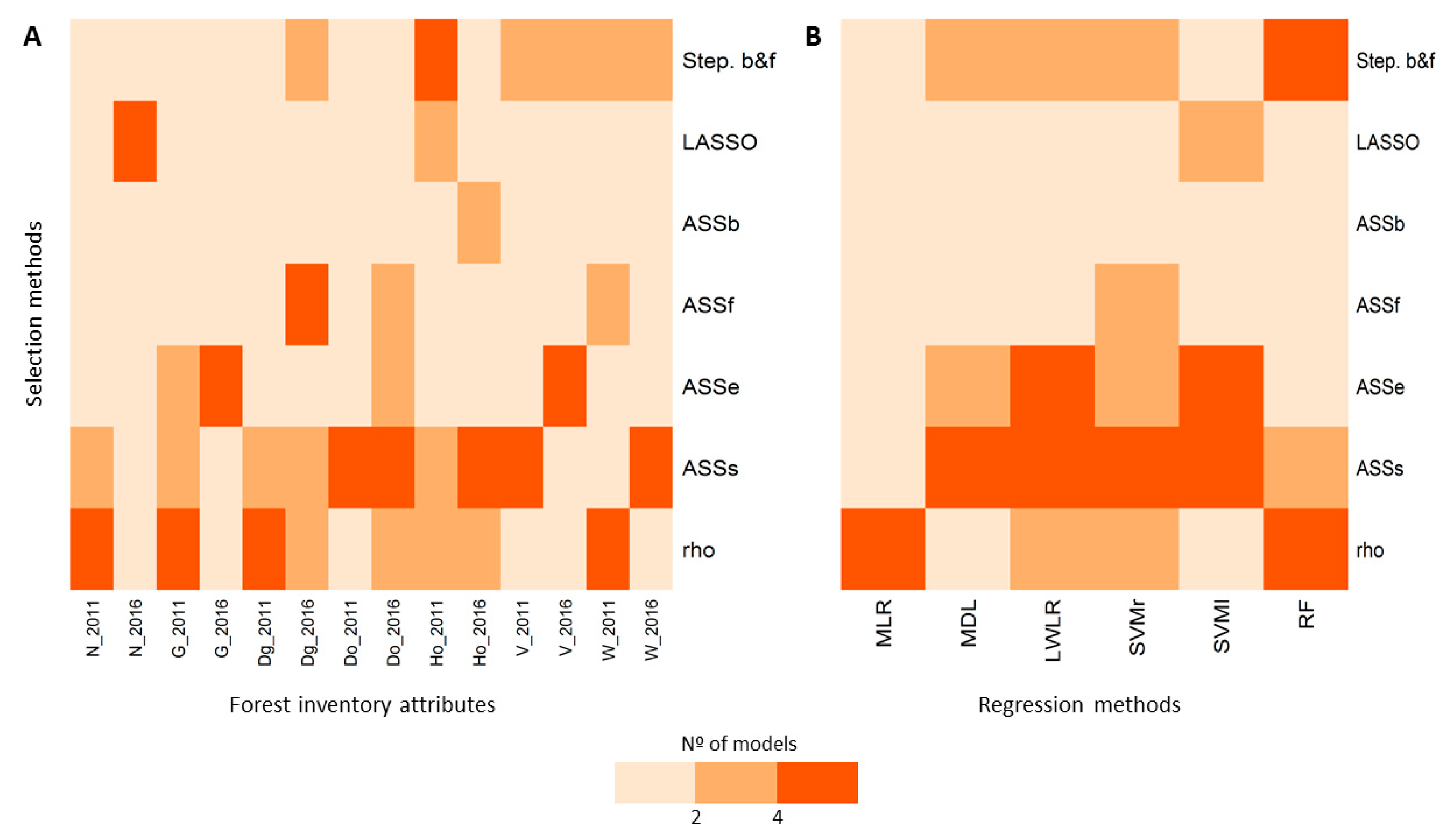
3.2. Variable Selection

This section includes the results of the selection of ALS variables for the seven estimated forestry attributes modeled with the different regression methods.

Figure 3A synthetizes the performance of the analyzed selection methods for each forest stand attributes by year. All subsets regression Seqrep (ASSs) was the most powerful selection method. Spearman’s rank correlation (rho) coefficient also showed good results, especially for selecting N, G, Dg, and W in 2011. All subsets regression Exhaustive (ASSe) and Stepwise (Step b&f) were both good selection methods for estimating G, Ho, and V. However, lasso selection (LASSO), all subsets regression Backward (ASSb) and all subsets regression Forward (ASSf) have been less utilized. The stepwise forward and PCA selection methods have not been included in Figure 3 as they did not determine the best variables for modeling in any of the cases. For detailed information of the selection methods performance, see

Table A2. Summary of the N models using 2011 ALS data. Validation results in terms of RMSE (stems ha⁻¹), %RMSE, and bias (stems ha⁻¹) and R². SM refers to selection method; Step. stands for Stepwise both and forward; SVMr. refers to support vector machine with radial kernel; SVM l. refers to support vector machine with linear kernel; ret. refers to returns.

			Fitting Phase			Validation
ALS Metrics	Model	SM	RMSE	% RMSE	Bias	RMSE	% RMSE	Bias	R2
P90 + (All ret. above mean)/(total first ret.) × 100	MLR	Step.	347.22	49.08	0.00	350.67	49.57	8.76	0.53
Elev. L2 + Elev. Variance + (All ret. above 2.00)/(total first ret.) × 100	MDL	ASSs	235.89	33.34	−0.83	292.37	41.33	−1.48	0.68
P99 + Elev. IQ + % first ret. above 2.00	LWLR	Rho	205.80	29.09	−9.79	310.97	43.96	−11.39	0.65
P99 + Elev. IQ + % first ret. above 2.00	SVMr	rho	257.09	36.34	28.81	272.76	38.55	26.99	0.72
Elev. L2 + Elev. Variance + (All ret. above 2.00)/(total first ret.) × 100	SVMl	ASSs	319.34	45.14	60.68	309.56	43.76	64.83	0.65
P99 + Elev. SD + % first ret. above 2.00	RF	rho	151.86	21.46	1.91	303.56	42.91	6.91	0.66

,

Table A3. Summary of the N models using 2016 ALS data. Validation results in terms of RMSE (stems ha⁻¹), %RMSE, and bias (stems ha⁻¹) and R². SM refers to selection method; Step. stands for Stepwise both and forward; SVMr. refers to support vector machine with radial kernel; SVM l. refers to support vector machine with linear kernel; ret. refers to returns.

			Fitting Phase			Validation
ALS Metrics	Model	SM	RMSE	% RMSE	Bias	RMSE	% RMSE	Bias	R2
Elev. mean + Elev. L kurtosis + Canopy relief ratio	MLR	Step.	358.84	51.47	0.00	363.62	52.15	11.57	0.45
Elev. maximum + Elev. L kurtosis + % first ret. above 2.00	MDL	LASSO	243.13	34.87	1.14	322.89	46.31	8.15	0.61
Elev. maximum + Elev. L kurtosis + % first ret. above 2.00	LWLR	LASSO	204.63	29.35	4.55	333.20	47.79	11.06	0.57
Elev. maximum + Elev. L kurtosis + % first ret. above 2.00	SVMr	LASSO	250.87	35.98	13.95	278.58	39.96	11.83	0.67
Elev. maximum + Elev. L kurtosis + % first ret. above 2.00	SVMl	LASSO	322.11	46.20	29.31	313.41	44.95	36.04	0.59
Elev. maximum + Elev. L kurtosis + % first ret. above 2.00	RF	LASSO	159.15	22.83	−1.71	302.57	43.40	−10.81	0.60

,

Table A4. Summary of the G models using 2011 ALS data. Validation results in terms of RMSE (m² ha⁻¹), %RMSE, and bias (m² ha⁻¹) and R². SM refers to selection method; Step. stands for Stepwise both and forward; SVMr. refers to support vector machine with radial kernel; SVM l. refers to support vector machine with linear kernel; ret. refers to returns.

			Fitting Phase			Validation
ALS Metrics	Model	SM	RMSE	% RMSE	Bias	RMSE	% RMSE	Bias	R2
Elev. minimum + Elev. Kurtosis + (All ret. above mode)/(total first ret.) × 100	MLR	rho	5.80	29.80	0.00	6.01	30.89	0.19	0.64
P10 + % first ret. above 2.00	MDL	rho	4.61	23.69	0.21	5.23	26.85	0.38	0.74
P05 + % first ret. above mean	LWLR	ASSe	4.07	20.92	0.01	5.53	28.42	0.12	0.70
Elev. minimum + Elev. Kurtosis + (All ret. above mode)/(total first ret.) × 100	SVMr	ASSs	4.43	22.77	−0.10	4.77	24.51	−0.10	0.77
Elev. minimum + Elev. Kurtosis + (All ret. above mode)/(total first ret.) × 100	SVMl	ASSs	4.85	24.92	0.10	4.87	25.05	0.05	0.75
P10 + % first ret. above 2.00	RF	rho	2.61	13.41	0.02	5.19	26.69	0.06	0.73

,

Table A5. Summary of the G models using 2016 ALS data. Validation results in terms of RMSE (m² ha⁻¹), %RMSE, and bias (m² ha⁻¹) and R². SM refers to selection method; Step. stands for Stepwise both and forward; SVMr. refers to support vector machine with radial kernel; SVM l. refers to support vector machine with linear kernel; ret. refers to returns.

			Fitting Phase			Validation
ALS Metrics	Model	SM	RMSE	% RMSE	Bias	RMSE	% RMSE	Bias	R2
Elev. minimum +% all ret. above mode	MLR	rho	9.27	42.11	0.00	9.19	41.76	0.21	0.15
P75 + Elev. CUR mean CUBE + (All ret. above 2.00)/(total first ret.) × 100	MDL	ASSe	3.65	16.57	0.19	4.43	20.11	0.12	0.82
P75 + Elev. CUR mean CUBE + (All ret. above 2.00)/(total first ret.) × 100	LWLR	ASSe	2.84	12.93	0.01	5.05	22.94	−0.10	0.77
P75 + Elev. CUR mean CUBE + (All ret. above 2.00)/(total first ret.) × 100	SVMr	ASSe	3.88	17.61	0.41	4.14	18.80	0.30	0.84
P75 + Elev. CUR mean CUBE + (All ret. above 2.00)/(total first ret.) × 100	SVMl	ASSe	4.38	19.89	0.44	4.43	20.12	0.35	0.81
P10 + Elev. minimum + % first ret. above mean	RF	ASSf	2.32	10.56	0.08	4.64	21.06	0.37	0.81

,

Table A6. Summary of the Dg models using 2011 ALS data. Validation results in terms of RMSE (cm), %RMSE, and bias (cm) and R². SM refers to selection method; Step. stands for Stepwise both and forward; SVMr. refers to Support Vector Machine with radial kernel; SVM l. refers to Support Vector Machine with linear kernel; ret. refers to returns.

			Fitting Phase			Validation
ALS Metrics	Model	SM	RMSE	% RMSE	Bias	RMSE	% RMSE	Bias	R2
P90 + % first ret. above mean	MLR	rho	3.80	18.44	0.00	3.84	18.60	−0.03	0.77
P90 + (All ret. above 2.00)/(total first ret.) × 100	MDL	ASSs	3.30	15.97	0.16	3.78	18.34	0.00	0.78
P90 + (All ret. above 2.00)/(total first ret.) × 100	LWLR	ASSs	2.98	14.46	−0.02	3.75	18.19	−0.22	0.78
P90 + Elev. Std.dev + % first ret. above mean	SVMr	rho	3.38	16.38	0.19	3.56	17.25	0.06	0.81
P90 + Elev. Std.dev + % first ret. above mean	SVMl	rho	3.76	18.24	0.08	3.88	18.80	−0.06	0.78
P90 + Elev. Std.dev + (All ret. above mean)/(total first ret.) × 100	RF	rho	1.89	9.17	−0.02	3.75	18.18	−0.04	0.79

,

Table A7. Summary of the Dg models using 2016 ALS data. Validation results in terms of RMSE (cm), %RMSE, and bias (cm) and R². SM refers to selection method; Step. stands for Stepwise both and forward; SVMr. refers to Support Vector Machine with radial kernel; SVM l. refers to Support Vector Machine with linear kernel; ret. refers to returns.

			Fitting Phase			Validation
ALS Metrics	Model	SM	RMSE	% RMSE	Bias	RMSE	% RMSE	Bias	R2
P90 + Elev. LCV + (All ret. above mean)/(total first ret.) × 100	MLR	Step.	3.48	15.53	0.00	3.63	16.22	−0.07	0.82
Elev. maximum + Elev. IQ + (All ret. above 2.00)/(total first ret.) × 100	MDL	ASSf	3.12	13.93	0.23	3.71	16.58	0.21	0.82
P90 + Elev. LCV + (All ret. above mean)/(total first ret.) × 100	LWLR	Step.	2.59	11.58	−0.03	3.91	17.48	−0.04	0.80
Elev. maximum + Elev. IQ + (All ret. above 2.00)/(total first ret.) × 100	SVMr	ASSf	3.03	13.53	0.21	3.42	15.28	0.11	0.85
P90 + Elev. mode + % first ret. above mode	SVMl	ASSs	3.45	15.40	0.20	3.57	15.95	0.11	0.83
P90 + Elev. LCV + (All ret. above mean)/(total first ret.) × 100	RF	rho	1.65	7.39	0.01	3.59	16.05	0.05	0.82

,

Table A8. Summary of the Do models using 2011 ALS data. Validation results in terms of RMSE (cm), %RMSE, and bias (cm) and R². SM refers to selection method; Step. stands for Stepwise both and forward; SVMr. refers to Support Vector Machine with radial kernel; SVM l. refers to Support Vector Machine with linear kernel; ret. refers to returns.

			Fitting Phase			Validation
ALS Metrics	Model	SM	RMSE	% RMSE	Bias	RMSE	% RMSE	Bias	R2
Elev. skewness + Elev. Lkurtosis + P25	MLR	rho	5.34	20.17	0.00	5.42	20.47	0.07	0.62
P90+ (All ret. above 2.00)/(total first ret.) × 100	MDL	ASSf	3.99	15.07	0.10	4.27	16.12	0.11	0.77
P90+ (All ret. above 2.00)/(total first ret.) × 100	LWLR	ASSf	3.49	13.17	−0.03	4.29	16.19	−0.05	0.77
P90+ (All ret. above 2.00)/(total first ret.) x 100	SVMr	ASSf	4.11	15.53	0.19	4.07	15.36	0.11	0.79
P90+ (All ret. above 2.00)/(total first ret.) × 100	SVMl	ASSf	4.24	16.01	0.22	4.20	15.85	0.11	0.78
P90 + % first ret. above mean	RF	rho	2.13	8.04	−0.11	4.38	16.55	−0.36	0.76

,

Table A9. Summary of the Do models using 2016 ALS data. Validation results in terms of RMSE (cm), %RMSE, and bias (cm) and R². SM refers to selection method; Step. stands for Stepwise both and forward; SVMr. refers to support vector machine with radial kernel; SVM l. refers to support vector machine with linear kernel; ret. refers to returns.

			Fitting Phase			Validation
ALS Metrics	Model	SM	RMSE	% RMSE	Bias	RMSE	% RMSE	Bias	R2
P90 + Elev. CV + (All ret. above mean)/(total first ret.) × 100	MLR	Step.	3.53	12.33	0.00	3.63	12.68	−0.08	0.85
P90 + Elev. variance + Elev. L2	MDL	ASSs	3.26	11.40	0.18	3.47	12.13	0.23	0.86
P95 + Elev. CV	LWLR	ASSs	2.88	10.07	−0.03	3.63	12.70	−0.09	0.84
P95 + Elev. CV	SVMr	ASSs	3.25	11.35	0.40	3.40	11.89	0.33	0.87
Elev. Std.dev + Elev. Variance + P05	SVMl	ASSe	3.26	11.40	0.18	3.36	11.75	0.11	0.87
P95 + Elev. CV	RF	ASSs	1.61	5.64	−0.02	3.62	12.64	0.00	0.85

,

Table A10. Summary of the Ho models using 2011 ALS data. Validation results in terms of RMSE (m), %RMSE, and bias (m) and R². SM refers to selection method; Step. stands for Stepwise both and forward; SVMr. refers to Support Vector Machine with radial kernel; SVM l. refers to Support Vector Machine with linear kernel; ret. refers to returns.

			Fitting Phase			Validation
ALS Metrics	Model	SM	RMSE	% RMSE	Bias	RMSE	% RMSE	Bias	R2
Elev. LCV + Elev. Lkurtosis + P01	MLR	rho	2.21	20.24	0.00	2.26	20.71	0.05	0.63
P90 + Elev. kurtosis	MDL	Step.	1.24	11.36	0.10	1.44	13.18	0.08	0.85
P90 + Elev. skewness	LWLR	ASSs	1.16	10.69	−0.02	1.40	12.83	0.01	0.86
P90 + Elev. variance + % All ret. above mean	SVMr	ASSf	1.32	12.11	0.11	1.34	12.30	0.09	0.87
Elev. L1 + Elev. maximum	SVMl	LASSO	1.42	12.99	0.09	1.40	12.82	0.05	0.86
P90 + Canopy relief ratio	RF	Step.	0.72	6.65	−0.01	1.46	13.41	−0.06	0.84

,

Table A11. Summary of the Ho models using 2016 ALS data. Validation results in terms of RMSE (m), %RMSE, and bias (m) and R². SM refers to selection method; Step. stands for Stepwise both and forward; SVMr. refers to Support Vector Machine with radial kernel; SVM l. refers to Support Vector Machine with linear kernel; ret. refers to returns.

			Fitting Phase			Validation
ALS Metrics	Model	SM	RMSE	% RMSE	Bias	RMSE	% RMSE	Bias	R2
Elev. minimum + Elev. CV + Canopy relief ratio	MLR	rho	2.41	20.90	0.00	2.52	21.91	0.01	0.51
P95 + Elev. Std.dev	MDL	ASSs	0.92	7.99	0.07	0.95	8.27	0.07	0.93
P95 + Elev. variance	LWLR	ASSs	0.79	6.87	0.02	0.98	8.48	0.00	0.93
P95 + Elev. Std.dev	SVMr	ASSs	0.86	7.48	0.03	1.02	8.83	0.03	0.92
P90 + Elev. variance + Elev. SQRT mean SQ	SVMl	ASSb	0.96	8.30	0.12	1.00	8.69	0.08	0.93
P95 + Elev. variance + (All ret. above mean)/(total first ret.) × 100	RF	rho	0.43	3.76	−0.01	1.00	8.72	−0.03	0.92

,

Table A12. Summary of the V models using 2011 ALS data. Validation results in terms of RMSE (m³ ha⁻¹), %RMSE, and bias (m³ ha⁻¹) and R². SM refers to selection method; Step. stands for Stepwise both and forward; SVMr. refers to support vector machine with radial kernel; SVM l. refers to support vector machine with linear kernel; ret. refers to returns.

			Fitting Phase			Validation
ALS Metrics	Model	SM	RMSE	% RMSE	Bias	RMSE	% RMSE	Bias	R2
P20 + (All ret. above 2.00)/(total first ret.) × 100	MDL	ASSs	30.15	28.63	1.69	33.39	31.71	2.13	0.81
P20 + (All ret. above 2.00)/(total first ret.) × 100	LWLR	ASSs	25.89	24.58	0.05	34.09	32.37	0.24	0.80
Elev. L2 + Elev. CUR mean CUBE + % first ret. above mean	SVMr	Step.	28.87	27.42	2.59	29.71	28.22	1.79	0.84
P20 + Elev. L skewness + (All ret. above mean)/(total first ret.) × 100	SVMl	ASSs	34.25	32.52	0.88	34.30	32.58	0.09	0.79
P20 + Elev. L skewness + % first ret. above 2.00	RF	ASSs	16.80	15.96	0.17	34.28	32.55	−0.56	0.78

,

Table A13. Summary of the V models using 2016 ALS data. Validation results in terms of RMSE (m³ ha⁻¹), %RMSE, and bias (m³ ha⁻¹) and R². SM refers to selection method; Step. stands for Stepwise both and forward; SVMr. refers to support vector machine with radial kernel; SVM l. refers to support vector machine with linear kernel; ret. refers to returns.

			Fitting Phase			Validation
ALS Metrics	Model	SM	RMSE	% RMSE	Bias	RMSE	% RMSE	Bias	R2
P75 + Elev. CUR mean CUBE + (All ret. above 2.00)/(total first ret.) × 100	MDL	ASSe	24.87	20.02	−0.34	29.63	23.85	−0.19	0.88
P75 + Elev. CUR mean CUBE + (All ret. above 2.00)/(total first ret.) × 100	LWLR	ASSe	20.26	16.30	−0.08	31.80	25.59	−0.06	0.85
P75 + Elev. CUR mean CUBE + (All ret. above 2.00)/(total first ret.) × 100	SVMr	ASSe	24.69	19.87	2.65	26.35	21.20	1.92	0.90
P75 + Elev. CUR mean CUBE + (All ret. above 2.00)/(total first ret.) × 100	SVMl	ASSe	30.49	24.54	2.60	31.14	25.06	1.48	0.86
Elev. L2 + Elev. CUR mean CUBE + % first ret. above 2.00	RF	Step.	15.25	12.27	−0.38	31.73	25.53	0.32	0.86

,

Table A14. Summary of the W models using 2011 ALS data. Validation results in terms of RMSE (tons ha⁻¹), %RMSE, and bias (tons ha⁻¹) and R². SM refers to selection method; Step. stands for Stepwise both and forward; SVMr. refers to support vector machine with radial kernel; SVM l. refers to support vector machine with linear kernel; ret. refers to returns.

			Fitting Phase			Validation
ALS Metrics	Model	SM	RMSE	% RMSE	Bias	RMSE	% RMSE	Bias	R2
Elev. L2 + Elev. CUR mean CUBE + % first ret. above 2.00	MDL	Step.	22.02	24.21	0.68	28.30	31.12	1.82	0.76
P10 + Elev. CUR mean CUBE + % first ret. above mean	LWLR	rho	18.34	20.17	0.23	29.12	32.02	0.04	0.74
P10 + Elev. SQRT mean SQ + (All ret. above mean)/(total first ret.) × 100	SVMr	rho	23.00	25.29	0.75	24.29	26.71	−0.03	0.82
P10 + Canopy relief ratio + (All ret. above mean)/(total first ret.) × 100	SVMl	ASSf	26.60	29.25	0.50	26.82	29.49	0.11	0.79
P10 + Elev. CUR mean CUBE + (All ret. above mean)/(total first ret.) × 100	RF	rho	14.39	15.83	−0.05	29.43	32.36	0.24	0.75

and

Table A15. Summary of the W models using 2016 ALS data. Validation results in terms of RMSE (tons ha⁻¹), %RMSE, and bias (tons ha⁻¹) and R². SM refers to selection method; Step. stands for Stepwise both and forward; SVMr. refers to support vector machine with radial kernel; SVM l. refers to support vector machine with linear kernel; ret. refers to returns.

			Fitting Phase			Validation
ALS Metrics	Model	SM	RMSE	% RMSE	Bias	RMSE	% RMSE	Bias	R2
P75 + Elev. CUR mean CUBE + (All ret. above 2.00)/(total first ret.) × 100	MDL	ASSe	19.66	18.44	−0.64	23.44	21.98	−0.43	0.88
P75 + Elev. CUR mean CUBE + (All ret. above 2.00)/(total first ret.) × 100	LWLR	ASSe	16.11	15.11	−0.11	25.75	24.15	0.18	0.85
Elev. L2 + Elev. CUR mean CUBE + % first ret. above 2.00	SVMr	Step.	18.82	17.65	1.23	20.06	18.81	0.56	0.90
P75 + Elev. CUR mean CUBE + (All ret. above 2.00)/(total first ret.) × 100	SVMl	ASSe	22.78	21.37	1.65	23.43	21.98	0.80	0.87
P20 + Elev. CUR mean CUBE + All ret. above 2.00)/(total first ret.) × 100	RF	Step.	12.58	11.80	0.13	22.38	20.99	0.01	0.87

in the Appendix A.

Figure 3B depicts the performance of selection methods associated to each regression method without considering the year of the model. The ASSs was the most powerful method to select the best ALS metrics when using the MDL, LWLR, SVMr, and SVMl regression methods. Furthermore, rho coefficient was the most powerful one when using the MLR and RF regression methods. The ASSe and Step b&f both were also good selection techniques for almost all the regression methods, excluding MLR. However, LASSO, ASSb, and ASSf were less effective.

Figure 4 shows the ALS selected metrics for estimating the forest inventory attributes for both 2011 and 2016 years. As mentioned in Section 2.4, for better understanding of results, the ALS metrics are classified into groups (see Table A1 in Appendix A). In general, higher height variables, variability, and variables related to the ratio between all returns and total returns were included in most of the models, while height variables and variability L moments were less demanded. Comparing the different estimated forest attributes, some differences can be observed. N, Dg, and Do estimations included higher height variables, variability metrics, and CDM metrics. Ho estimation usually required higher height variables and variability metrics, while CDM metrics were not included. G, V, and W estimations included either lower or higher height metrics, variability metrics, and CDM ones.

3.3. Indirect Approach

The regression models to estimate Dg, Do, G, Ho, N, V, and W for 2011 and 2016 years using the indirect approach are summarized in Table A2, Table A3, Table A4, Table A5, Table A6, Table A7, Table A8, Table A9, Table A10, Table A11, Table A12, Table A13, Table A14 and Table A15 of the Appendix A. Figure 5 summarizes the %RMSE respect to the mean of the different regression methods for estimating the forest inventory attributes. Models developed for 2016 (Figure 5B) present generally higher accuracy than the ones generated for 2011 (Figure 5A). The point density of ALS datasets may determine these differences in accuracy. The SVMr shows the lower RMSE when modeling all the analyzed stand attributes in 2011 (Figure 5A). In this year, SVMl was the second best model when estimating Do, G, Ho, and W; MDL when estimating N and V; and RF when estimating Dg. The MLR regression method was not computed for V and W, as statistical assumptions of linear regression were not fulfilled, even considering logarithmic transformation. The MLR shows the lowest accuracy when estimating Do, G, Ho, and N.

The SVMr is the best model for estimating N, V, W, Dg, and G in 2016 (Figure 5B). However, in this year, SVMl and MDL outperformed SVMr when estimating Do and Ho, respectively. In 2016, MLR shows the lowest accuracy when estimating G, Ho, and N.

Friedman tests shows that the models are not equivalent, with a p-value lower than 0.05 when testing whether there were statistically significant differences between regression methods for 2011 and 2016 years. Thereby, the post-hoc Nemenyi test indicates that no statistically significant differences exist between the methods, with 95% of probability, except for MLR. In this sense, statistically significant differences were found when comparing models in the following cases: between MLR and SVMr models when estimating Do and G for 2011; between MLR and MDL models when estimating Ho for 2011; between MLR and MDL models when estimating Dg for 2016; and between MLR and all the generated models when estimating G, Ho, and N for 2016.

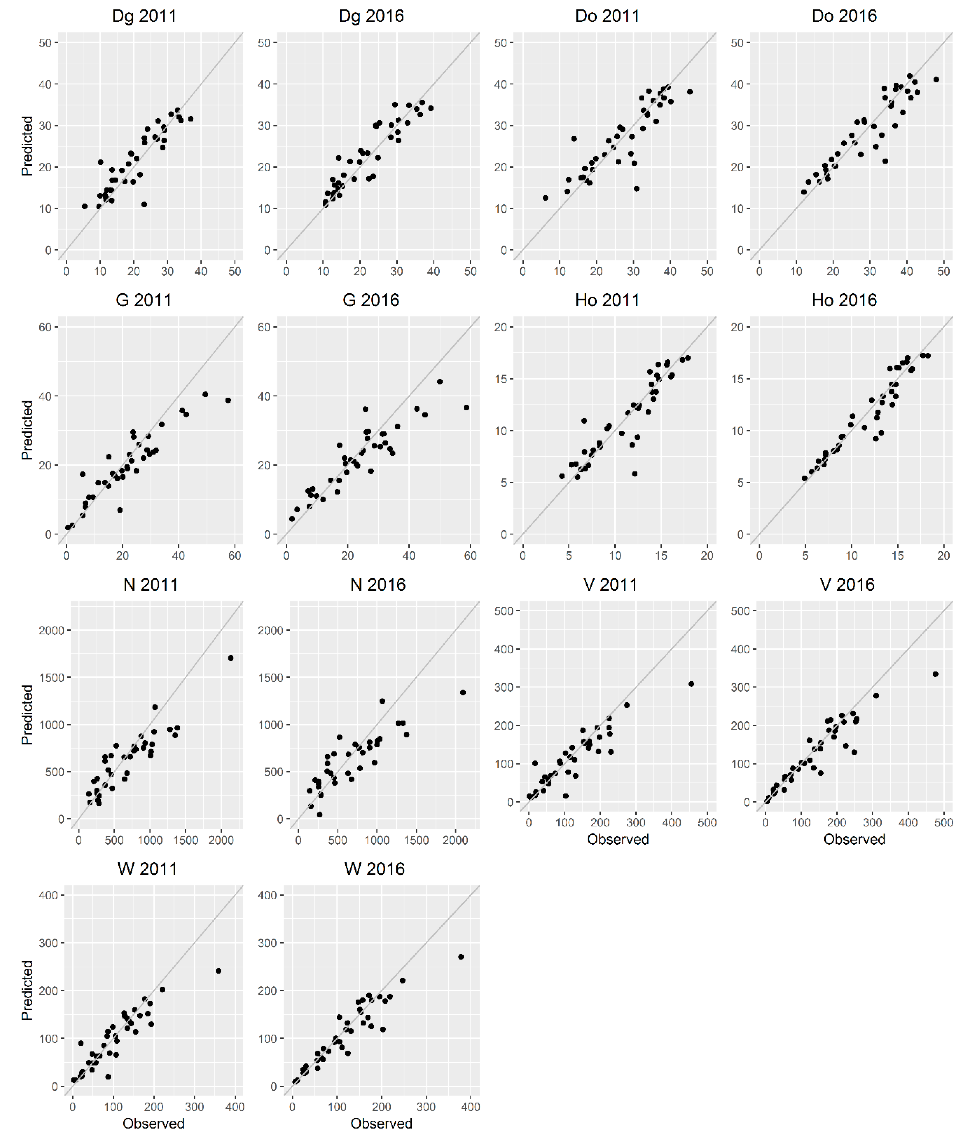
3.4. Direct Approach

The SVMr was established as the regression method for analyzing how models fitted at 2011 perform at 2016, and inversely, following a direct approach to analyze temporal transferability. This method resulted the best estimator for all the models generated in 2011 and for the majority of forest attributes modeled in 2016.

Table 5. Summary of the best-selected SVMr 2011 models and 2016 extrapolated ones. ret. refers to returns; e is extrapolated; N is stand density; G is basal area; Dg is squared mean diameter; Do is dominant diameter; Ho is dominant height; V is timber volume over bark of stem; W is total tree biomass.

		Fitting Phase			Validation
Attribute	ALS Metrics	RMSE	% RMSE	Bias	RMSE	% RMSE	Bias	R2
N 2011 N 2016e	P99 + ElevIQ + % first ret. Above 2.00	257.09	36.34	28.81	272.76	38.55	26.99	0.72
		265.62	38.10	17.99	295.83	42.43	20.49	0.64
G 2011 G 2016e	Elev. minimum + Elev. kurtosis + % first ret. above mean	4.43	22.77	−0.10	4.77	24.51	−0.10	0.77
		4.18	19.01	0.20	5.51	25.05	0.57	0.71
Dg 2011 Dg 2016e	P90 + Elev. SD + % first ret. above mean	3.38	16.38	0.19	3.56	17.25	0.06	0.81
		3.02	13.48	0.19	3.43	15.35	0.06	0.85
Do 2011 Do 2016e	P90 + (All ret. Above 2)/(total first ret) × 100	4.11	15.53	0.19	4.07	15.36	0.11	0.79
		3.43	11.99	0.41	3.53	12.33	0.31	0.86
Ho 2011 Ho 2016e	P90 + Elev. variance + % all ret. above mean	1.32	12.11	0.11	1.34	12.30	0.09	0.87
		0.86	7.47	0.10	0.98	8.54	0.10	0.93
V 2011 V 2016e	Elev. L2 + Elev. cubic mean + % first ret. above mean	28.87	27.42	2.59	29.71	28.22	1.79	0.84
		25.03	20.15	3.14	26.00	20.92	2.64	0.90
W 2011	P10 + Elev. Quadratic mean + (All ret. Above mean)/(total first ret) × 100	23.00	25.29	0.75	24.29	26.71	−0.03	0.82
W 2016e		19.63	18.41	1.80	21.39	20.06	1.08	0.89

summarizes the best-selected SVMr models fitted in 2011 and the ones extrapolated to 2016 by using the same ALS metrics and model parameters.

Table 6. Summary of the best-selected SVMr 2016 models and 2011 extrapolated ones. ret. refers to returns; e is extrapolated; N is stand density; G is basal area; Dg is squared mean diameter; Do is dominant diameter; Ho is dominant height; V is timber volume over bark of stem; W is total tree biomass.

		Fitting Phase			Validation
Attribute	ALS Metrics	RMSE	% RMSE	Bias	RMSE	% RMSE	Bias	R2
N 2011e	Elev. maximum + Elev. L kurtosis + % first ret. Above 2.00	256.69	36.28	33.73	340.20	48.09	49.31	0.55
N 2016		250.87	35.98	13.95	278.58	39.96	11.83	0.67
G 2011e	P75 + Elev. CUR mean CUBE + (All ret. Above 2)/(total first ret) × 100	4.97	25.54	0.26	5.04	25.88	0.13	0.74
G 2016		3.88	17.61	0.41	4.14	18.80	0.30	0.84
Dg 2011e	Elev. maximum + Elev. IQ + (All ret. Above 2)/(total first ret) × 100	3.54	17.14	0.14	3.77	18.25	0.00	0.79
Dg 2016		3.03	13.53	0.21	3.42	15.28	0.11	0.85
Do 2011e	P99 + Elev. CV	4.20	15.85	0.25	4.18	15.79	0.16	0.78
Do 2016		3.25	11.35	0.40	3.40	11.89	0.33	0.87
Ho 2011e	P95 + Elev. SD	1.32	12.12	0.03	1.38	12.64	0.03	0.86
Ho 2016		0.86	7.48	0.03	1.02	8.83	0.03	0.92
V 2011e	P75 + Elev. CUR mean CUBE + (All ret. Above 2)/(total first ret) × 100	29.97	28.46	1.51	30.96	29.40	0.84	0.83
V 2016		24.69	19.87	2.65	26.35	21.20	1.92	0.90
W 2011e	Elev. L2 + Elev. CUR mean CUBE + % first ret. Above 2.00	23.11	25.42	0.96	23.36	25.69	0.27	0.83
W 2016		18.82	17.65	1.23	20.06	18.81	0.56	0.90

summarizes the best-selected SVMr models fitted in 2016 and extrapolated to 2011 by using the same ALS metrics and model parameters. Furthermore, scatter plots of observed and predicted values for the analyzed forest stand attributes for both years are included in Figure A1 and Figure A2 of Appendix A.

In the case of the models fitted in 2011 and extrapolated to 2016 (Table 5), the %RMSE after validation ranges from 8.54 to 42.43% and R² ranges from 0.64 to 0.93 within the different stand attributes. As it is shown in Table 5, models are transferable. In fact, the average %RMSE differences between the fitted and the extrapolated models is 3.87%. Dg, Do, Ho, V, and W estimations for 2011 models have higher %RMSE than the one for models extrapolated to 2016. However, N and G models show higher %RMSE for the 2016 extrapolated ones.

In the case of the models fitted in 2016 and extrapolated to 2011 (Table 6), the %RMSE in the validation sample ranges from 8.83 to 48.09% and R² ranges from 0.55 to 0.92 within the different stand attributes. These models also show good temporal transferability, being the average %RMSE differences between the fitted and the extrapolated model 5.85%, even lower than the models fitted in 2011 and extrapolated to 2016. All the models fitted in 2016 for the analyzed stand attributes present lower RMSE than the ones extrapolated to 2011.

The comparison between fitted models generated for either 2011 or 2016 and the extrapolated ones were assessed using Friedman and post-hoc Nemenyi tests. Friedman test shows that the models for the analyzed stand attributes are not equivalent with a p-value lower than 0.05 when testing whether there were differences: (i) between models fitted in 2011 and the ones extrapolated to 2016; (ii) between models fitted in 2016 and the ones extrapolated to 2011; (iii) between models fitted in 2011 and models fitted in 2016; (iv) between models fitted in 2011 and models extrapolated to 2011; (v) between models fitted in 2016 and models extrapolated to 2016. Thereby, the required application of the post-hoc Nemenyi test indicates that no statistically significant differences exist between the methods for the proposed hypothesis, with 95% of probability.

4. Discussion

Airborne laser scanning is considered the best technology for mapping 3D vegetation structures [3] allowing the measurement of fine-scale forestry metrics [82]. Multi-temporal ALS data has been less explored as the availability of two or more LiDAR surveys in the same area is still limited. Nevertheless, several studies have used multi-temporal small-footprint ALS to estimate total tree biomass or carbon dynamics [3,9,21,22,23,24,25,26,27], volume changes [17,21], height growth [14,15,16,17,18,19], and basal area [17]. This study estimates seven forest attributes (N, G, Dg, Do, Ho, V, W) using bi-temporal low-point density ALS data in Mediterranean Aleppo pine heterogeneous forests. The high number of field plots has allowed estimating the seven mentioned forest attributes for 18.7% of the forested area in Aragón, providing results at a regional scale. Moreover, model temporal transferability was demonstrated which could improve forest management in a cost-effective way in Mediterranean Aleppo pine forests.

Multi-temporal LiDAR estimations of forest attributes requires the support of accompanying field surveys [3] being desirable to have them corresponding to LiDAR surveys [9]. Field surveys are cost and time demanding specially when acquiring a high number of plots. The use of specific individual-tree growth equations, derived from dbh growth by extracting tree cores or from interval or permanent plots, is a good way to get value from field plot inventories acquired between different ALS surveys. Diameter at breast height and height growth values from general yield tables from the Spanish National Forest Inventory have been applied in other studies for estimating total tree biomass in Aleppo pine forests [36]. Nevertheless, in this work specific single-tree growth models, generalized height-diameter curves and taper equations were used to estimate all stand attributes in the measured field plots at two different points in time, which produces more accurate results, particularly when predicting at short term [83].

The use of selection methods reduces variable collinearity, modeling time and increases model parsimony. All subset selection Seqrep was the most powerful selection method in agreement with Hansen et al. [84] who also used similar best subset regression procedures to estimate biomass with ALS data. Spearman rho coefficients, proposed as a good tool for determining the relationships between ALS and field metrics by Kristensen et al. [85], also showed a good result, agreeing with our previous studies [37]. Furthermore, our results agree with García-Gutiérrez et al. [78], who found that stepwise was a powerless technique. Accordingly, the use of automatic selection methods such as ASSs is proposed when using MDL, LWLR, SVMr, and SVMl regression methods in Mediterranean Aleppo pine forest. Nevertheless, comparison between selection methods should be considered when working with other forest types or species. In this sense, Rho coefficients should be considered specially when using MLR and RF regression methods and PCA should be taken into account for a first attempt to reduce collinearity as proposed by Naesset [54] and Cao et al. [9], but afterwards another selection approach should be considered before modeling.

The most selected types of ALS metrics for estimating the seven analyzed stand attributes were higher height variables, variability ones and the ratio between all returns and total returns, while dominant height and variability L moment variables where less demanded. Ho estimation usually required the inclusion of high height percentiles as concluded by Næsset and Gobakken [17]. V and W estimations normally included either lower or higher height variables, variability metrics, and/or CDM ones as proposed by Silva et al. [86] and Hopkinson et al. [87].

The comparison between regression methods shows that SVMr had the lowest RMSE when estimating the majority of the analyzed stand attributes for both dates, except for Do and Ho when using 2016 data. These results match with García-Gutiérrez et al. [78] and Guerra-Hernández et al. [38,88], which obtained higher accuracies when using non-parametric regression methods. Different results were found in our previous studies [36,89] as MLR slightly outperformed other nonparametric methods when estimating total tree biomass in Aleppo pine forests, but no statistically significant differences were found. Thus, in agreement with Gagliasso et al. [90], a high number of field plots may have boosted machine-learning performance. Furthermore, the broad range and standard deviation values of the field plot data that characterizes Aleppo pine forest at a regional scale is notoriously higher than in our previous studies. Thus, although logarithmic transformation of the dependent and independent variables was carried out, most of the data was not normally distributed. The limitation on using the best-suited ALS metrics, as most of them were not normally distributed, generates a considerable decrease of accuracy in MLR model performance. In this sense, comparison between regression methods is desirable, especially when working with big datasets in heterogeneous forest stands as the Mediterranean ones.

The comparison of direct and indirect approaches allowed us to assess model temporal transferability between 2011 and 2016. The direct approach was computed when extrapolating 2011 models to 2016 and inversely. The indirect approach has shown slightly better results when estimating N, G, Dg, Do, and V. Direct approach showed slightly better results in the estimation of W when extrapolating 2016 model to 2011, but not inversely. Similar results were found for the estimation of Ho when extrapolating 2011 model to 2016 data, but not inversely. Comparisons with previous studies cannot be done for N, Dg, and Do, as these attributes have not been previously estimated using multi-temporal data. Comparisons between Ho, G, and V results are neither possible as Næsset and Gobakken [17] performed only the indirect approach. Regarding W estimations, several results have been obtained using different regression methods, and even in our work both direct and indirect approaches performed in a different way when extrapolating the first-year model (2011) or the second one (2016). The indirect approach obtained better results when estimating W for 2011 data agreeing with Zhao et al. [3] and Meyer et al. [25]. Our results also agree with Cao et al. [9], Skowronski et al. [24], and Bollandsås et al. [26], which detected slightly better performance of direct approach. Similar results have been found in our study when extrapolating 2016 model to 2011. In general, the SVMr regression method shows good temporal transferability between both ALS acquisitions with average %RMSE differences for all the modeled stand attributes of 2.13% for 2011 and 1.58% for 2016.

Models generated using 2016 data (1.25 points m⁻²) showed generally higher accuracy than 2011 ones (0.64 points m⁻²). However, no statistically significant differences were found between the best-fitted models for each year. In agreement with Cao et al. [9], point density may influence model performance but did not significantly affect the estimations of forest attributes as point clouds has a consistent vertical pattern. According to Hudak et al. [27], the relatively large size of the sample plots is considered sufficient for generating canopy height metrics. Thus, the results confirm, as other previous studies based on low-density ALS from the Spanish National Plan for Aerial Orthophotography data (i.e., [33,36,37,38]), that this information is an accurate and economic alternative to perform forest inventories when higher point density data are not available.

Overall, the use of low-point ALS data for two dates and single-tree growth models for generating temporally-concomitant field data provides accurate estimations of forest stand attributes in Mediterranean Aleppo pine forests. The indirect approach produced higher precision, but the direct approach, within those conditions, may reduce fieldwork and time of model parametrization. When using a direct approach it would not be necessary to create one model for two different points in time, as it will be possible to extrapolate a model generated for one date (validated with field data) to another date. Furthermore, the number of revisited field plots can be dismissed or even not required, when the time between ALS surveys is not large [28]. This will benefit not only forest managers but also enterprises devoted to forest inventories. The use of direct method and the possibility of model temporal transferability generates new alternatives to calibrate future ALS captures with a lower number of field plots and helps in designing the temporal gap between flights. Single-tree growth models constitute a useful and robust alternative to update field data to a point in time, allowing to accurately estimate forest inventory parameters with the use of ALS data. Future research using multi-temporal ALS data should focus on the inclusion of inference models to better understand uncertainties as well as on the analysis of field plot size and saturation effects in model accuracy. Furthermore, the analysis of forests structural biodiversity changes caused by wildfires or the fusion of ALS data with multi-temporal passive remote sensing series or unmanned aerial vehicle (UAV) point clouds may help to monitor forest dynamics over time.

5. Conclusions

Multi-temporal ALS data may improve forest management and planning, providing accurate forest inventory attribute estimations for different points in time. The results illustrate the usefulness of bitemporal low-point density ALS data and single-tree growth models, when lacking temporally-concomitant field campaigns, to accurately estimate seven forestry attributes, using an area-based approach. All subsets regression Seqrep was the most powerful selection method, followed by rho coefficient, to generate parsimonious models. Higher height metrics, canopy height variability, and canopy density variables were the most selected ALS-metrics, while mean height variables and variability L moments were less demanded. The SVM with radial kernel outperformed the analyzed non-parametric and multivariate linear regression methods for estimating all forest inventory attributes except from Do and Ho when using 2016 data. Thus, machine-learning performance may have been boosted by forest heterogeneity and an elevated number of field plots.

This study has assessed model temporal transferability by comparing direct and indirect approaches for the estimation of seven forestry attributes. Indirect approach have produced slightly more accurate results than the direct approach, but average %RMSE differences between both approaches for all modeled stand attributes ranged from 2.13% in 2011 to 1.58% in 2016. Thus, mixing the direct approach with single-tree growth methods provides a suitable alternative to reduce fieldwork and enhance ALS technology as a good tool for estimating forest attributes in two different dates. The utility of multi-temporal ALS data and the combination with multi-temporal series from passive remote sensing and UAV point clouds derived by using photogrammetric techniques would have great value for forest management and planning.

References

1. Lal, R. Sequestration of atmospheric CO2 in global carbon pools. Energy Environ. Sci. 2008, 1, 86–100. [Google Scholar] [CrossRef]
2. Pan, Y.; Birdsey, R.A.; Fang, J.; Houghton, R.; Kauppi, P.E.; Kurz, W.A.; Phillips, O.L.; Shvidenko, A.; Lewis, S.L.; Canadell, J.G.; et al. A large and persistent carbon sink in the world’s forests. Science 2011, 333, 988–993. [Google Scholar] [CrossRef] [PubMed]
3. Zhao, K.; Suarez, J.C.; Garcia, M.; Hu, T.; Wang, C.; Londo, A. Utility of multitemporal lidar for forest and carbon monitoring: Tree growth, biomass dynamics, and carbon flux. Remote Sens. Environ. 2018, 204, 883–897. [Google Scholar] [CrossRef]
4. Zald, H.S.J.; Wulder, M.A.; White, J.C.; Hilker, T.; Hermosilla, T.; Hobart, G.W.; Coops, N.C. Integrating Landsat pixel composites and change metrics with lidar plots to predictively map forest structure and aboveground biomass in Saskatchewan, Canada. Remote Sens. Environ. 2016, 176, 188–201. [Google Scholar] [CrossRef] [Green Version]
5. Pflugmacher, D.; Cohen, W.B.; Kennedy, R.E.; Yang, Z. Using Landsat-derived disturbance and recovery history and lidar to map forest biomass dynamics. Remote Sens. Environ. 2014, 151, 124–137. [Google Scholar] [CrossRef]
6. Ferraz, A.; Saatchi, S.; Bormann, K.J.; Painter, T.H. Fusion of NASA Airborne Snow Observatory (ASO) Lidar Time Series over Mountain Forest Landscapes. Remote Sens. 2018, 10, 164. [Google Scholar] [CrossRef]
7. Hummel, S.; Hudak, A.T.; Uebler, E.H.; Falkowski, M.J.; Megown, K.A. A Comparison of Accuracy and Cost of LiDAR versus Stand Exam Data for Landscape Management on the Malheur National Forest. J. For. 2011, 109, 267–273. [Google Scholar]
8. Hudak, A.T.; Evans, J.S.; Stuart Smith, A.M. LiDAR Utility for Natural Resource Managers. Remote Sens. 2009, 1, 934–951. [Google Scholar] [CrossRef] [Green Version]
9. Cao, L.; Coops, N.C.; Innes, J.L.; Sheppard, S.R.J.; Fu, L.; Ruan, H.; She, G. Estimation of forest biomass dynamics in subtropical forests using multi-temporal airborne LiDAR data. Remote Sens. Environ. 2016, 178, 158–171. [Google Scholar] [CrossRef]
10. Dubayah, R.O.; Sheldon, S.L.; Clark, D.B.; Hofton, M.A.; Blair, J.B.; Hurtt, G.C.; Chazdon, R.L. Estimation of tropical forest height and biomass dynamics using lidar remote sensing at la Selva, Costa Rica. J. Geophys. Res. Biogeosci. 2010, 115, 1–17. [Google Scholar] [CrossRef]
11. Stoker, J.M.; Harding, D.; Parrish, J. The need for a national LIDAR dataset. Photogramm. Eng. Remote Sensing 2008, 74, 1066–1068. [Google Scholar]
12. Marinelli, D.; Paris, C.; Bruzzone, L. A Novel Approach to 3-D Change Detection in Multitemporal LiDAR Data Acquired in Forest Areas. IEEE Trans. Geosci. Remote Sens. 2018, 56, 3030–3046. [Google Scholar] [CrossRef]
13. Fekety, P.A.; Falkowski, M.J.; Hudak, A.T. Temporal transferability of LiDAR-based imputation of forest inventory attributes. Can. J. Forest Res. 2015, 45, 422–435. [Google Scholar] [CrossRef]
14. Socha, J.; Pierzchalski, M.; Bałazy, R.; Ciesielski, M. Modelling top height growth and site index using repeated laser scanning data. For. Ecol. Manag. 2017, 406, 307–317. [Google Scholar] [CrossRef]
15. Gatziolis, D.; Fried, J.S.; Monleon, V.S. Challenges to Estimating Tree Height via LiDAR in Closed-Canopy Forests: A Parable from Western Oregon. For. Sci. 2010, 56, 139–155. [Google Scholar]
16. Hopkinson, C.; Chasmer, L.; Hall, R.J. The uncertainty in conifer plantation growth prediction from multi-temporal lidar datasets. Remote Sens. Environ. 2008, 112, 1168–1180. [Google Scholar] [CrossRef]
17. Næsset, E.; Gobakken, T. Estimating forest growth using canopy metrics derived from airborne laser scanner data. Remote Sens. Environ. 2005, 96, 453–465. [Google Scholar] [CrossRef]
18. Yu, X.; Hyyppä, J.; Kaartinen, H.; Maltamo, M.; Hyyppä, H. Obtaining plotwise mean height and volume growth in boreal forests using multi-temporal laser surveys and various change detection techniques. Int. J. Remote Sens. 2008, 29, 1367–1386. [Google Scholar] [CrossRef]
19. Yu, X.; Hyyppä, J.; Hyyppä, H.; Maltamo, M. Effects of flight altitude on tree height estimation using airborne laser scanning. ISPRS Int. Arch. Photogramm. Remote Sens. Spat. Inf. Sci. 2004, XXXVI, 96–101. [Google Scholar]
20. St-Onge, B.; Vepakomma, U. Assessing forest gap dynamics and growth using multi-temporal laser-scanner data. ISPRS Int. Arch. Photogramm. Remote Sens. Spat. Inf. Sci. 2004, XXXVI, Par, 173–178. [Google Scholar]
21. Poudel, K.P.; Flewelling, J.W.; Temesgen, H. Predicting Volume and Biomass Change from Multi-Temporal Lidar Sampling and Remeasured Field Inventory Data in Panther Creek Watershed, Oregon, USA. Forests 2018, 9, 28. [Google Scholar] [CrossRef]
22. Temesgen, H.; Strunk, J.; Andersen, H.E.; Flewelling, J. Evaluating different models to predict biomass increment from multi-temporal lidar sampling and remeasured field inventory data in south-central Alaska. Math. Comput. For. Nat. Res. Sci. 2015, 7, 66–80. [Google Scholar]
23. Réjou-Méchain, M.; Tymen, B.; Blanc, L.; Fauset, S.; Feldpausch, T.R.; Monteagudo, A.; Phillips, O.L.; Richard, H.; Chave, J. Using repeated small-footprint LiDAR acquisitions to infer spatial and temporal variations of a high-biomass Neotropical forest. Remote Sens. Environ. 2015, 169, 93–101. [Google Scholar] [CrossRef] [Green Version]
24. Skowronski, N.S.; Clark, K.L.; Gallagher, M.; Birdsey, R.A.; Hom, J.L. Airborne laser scanner-assisted estimation of aboveground biomass change in a temperate oak–pine forest. Remote Sens. Environ. 2014, 151, 166–174. [Google Scholar] [CrossRef]
25. Meyer, V.; Saatchi, S.S.; Chave, J.; Dalling, J.W.; Bohlman, S.; Fricker, G.A.; Robinson, C.; Neumann, M.; Hubbell, S. Detecting tropical forest biomass dynamics from repeated airborne lidar measurements. Biogeosciences 2013, 10, 5421–5438. [Google Scholar] [CrossRef]
26. Bollandsås, O.M.; Gregoire, T.G.; Næsset, E.; Øyen, B.H. Detection of biomass change in a Norwegian mountain forest area using small footprint airborne laser scanner data. Stat. Methods Appl. 2013, 22, 113–129. [Google Scholar] [CrossRef]
27. Hudak, A.T.; Strand, E.K.; Vierling, L.A.; Byrne, J.C.; Eitel, J.U.H.; Martinuzzi, S.; Falkowski, M.J. Quantifying aboveground forest carbon pools and fluxes from repeat LiDAR surveys. Remote Sens. Environ. 2012, 123, 25–40. [Google Scholar] [CrossRef]
28. Noordermeer, L.; Bollandsås, O.M.; Gobakken, T.; Næsset, E. Direct and indirect site index determination for Norway spruce and Scots pine using bitemporal airborne laser scanner data. For. Ecol. Manag. 2018, 428, 104–114. [Google Scholar] [CrossRef]
29. Mccarley, T.R.; Kolden, C.A.; Vaillant, N.M.; Hudak, A.T.; Smith, A.M.S.; Wing, B.M.; Kellogg, B.S.; Kreitler, J. Multi-temporal LiDAR and Landsat quantification of fire-induced changes to forest structure. Remote Sens. Environ. 2017, 419–432. [Google Scholar] [CrossRef]
30. Vepakomma, U.; Kneeshaw, D.; St-Onge, B. Interactions of multiple disturbances in shaping boreal forest dynamics: A spatially explicit analysis using multi-temporal lidar data and high-resolution imagery. J. Ecol. 2010, 98, 526–539. [Google Scholar] [CrossRef]
31. Vepakomma, U.; St-Onge, B.; Kneeshaw, D. Spatially explicit characterization of boreal forest gap dynamics using multi-temporal lidar data. Remote Sens. Environ. 2008, 112, 2326–2340. [Google Scholar] [CrossRef]
32. Solberg, S.; Næsset, E.; Hanssen, K.H.; Christiansen, E. Mapping defoliation during a severe insect attack on Scots pine using airborne laser scanning. Remote Sens. Environ. 2006, 102, 364–376. [Google Scholar] [CrossRef]
33. Guerra-Hernández, J.; Görgens, E.B.; García-Gutiérrez, J.; Rodriguez, L.C.E.; Tomé, M.; González-Ferreiro, E. Comparison of ALS based models for estimating aboveground biomass in three types of Mediterranean forest. Eur. J. Remote Sens. 2016, 49, 185. [Google Scholar] [CrossRef]
34. Mehtatalo, L.; Virolainen, A.; Tuomela, J.; Packalen, P. Estimating Tree Height Distribution Using Low-Density ALS Data With and Without Training Data. IEEE J. Sel. Top. Appl. Earth Obs. Remote Sens. 2015, 8, 1432–1441. [Google Scholar] [CrossRef]
35. Shendryk, I.; Hellström, M.; Klemedtsson, L.; Kljun, N. Low-Density LiDAR and Optical Imagery for Biomass Estimation over Boreal Forest in Sweden. Forests 2014, 5, 992–1010. [Google Scholar] [CrossRef] [Green Version]
36. Domingo, D.; Lamelas, M.; Montealegre, A.; García-Martín, A.; de la Riva, J.; Domingo, D.; Lamelas, M.T.; Montealegre, A.L.; García-Martín, A.; de la Riva, J. Estimation of Total Biomass in Aleppo Pine Forest Stands Applying Parametric and Nonparametric Methods to Low-Density Airborne Laser Scanning Data. Forests 2018, 9, 158. [Google Scholar] [CrossRef]
37. Montealegre, A.L.; Lamelas, M.T.; de la Riva, J.; García-Martín, A.; Escribano, F. Use of low point density ALS data to estimate stand-level structural variables in Mediterranean Aleppo pine forest. Forestry 2016, 89, 373–382. [Google Scholar] [CrossRef] [Green Version]
38. Garcia-Gutierrez, J.; Gonzalez-Ferreiro, E.; Riquelme-Santos, J.C.; Miranda, D.; Dieguez-Aranda, U.; Navarro-Cerrillo, R.M. Evolutionary feature selection to estimate forest stand variables using LiDAR. Int. J. Appl. Earth Obs. Geoinf. 2014, 26, 119–131. [Google Scholar] [CrossRef] [Green Version]
39. Jakubowski, M.K.; Guo, Q.; Kelly, M. Tradeoffs between lidar pulse density and forest measurement accuracy. Remote Sens. Environ. 2013, 130, 245–253. [Google Scholar] [CrossRef]
40. Gobakken, T.; Næsset, E. Assessing effects of laser point density, ground sampling intensity, and field sample plot size on biophysical stand properties derived from airborne laser scanner data. Can. J. For. Res. 2008, 38, 1095–1109. [Google Scholar] [CrossRef]
41. Lovell, J.L.; Jupp, D.L.B.; Newnham, G.J.; Coops, N.C.; Culvenor, D.S. Simulation study for finding optimal lidar acquisition parameters for forest height retrieval. For. Ecol. Manag. 2005, 214, 398–412. [Google Scholar] [CrossRef]
42. Roussel, J.-R.; Caspersen, J.; Béland, M.; Thomas, S.; Achim, A. Removing bias from LiDAR-based estimates of canopy height: Accounting for the effects of pulse density and footprint size. Remote Sens. Environ. 2017, 198, 1–16. [Google Scholar] [CrossRef]
43. Garcia, M.; Saatchi, S.; Casas, A.; Koltunov, A.; Ustin, S.; Ramirez, C.; Garcia-Gutierrez, J.; Balzter, H. Quantifying biomass consumption and carbon release from the California Rim fire by integrating airborne LiDAR and Landsat OLI data. J. Geophys. Res. Biogeosci. 2017. [Google Scholar] [CrossRef]
44. Singh, K.K.; Chen, G.; McCarter, J.B.; Meentemeyer, R.K. Effects of LiDAR point density and landscape context on estimates of urban forest biomass. ISPRS J. Photogramm. Remote Sens. 2015, 101, 310–322. [Google Scholar] [CrossRef]
45. Ruiz, L.; Hermosilla, T.; Mauro, F.; Godino, M.; Ruiz, L.A.; Hermosilla, T.; Mauro, F.; Godino, M. Analysis of the Influence of Plot Size and LiDAR Density on Forest Structure Attribute Estimates. Forests 2014, 5, 936–951. [Google Scholar] [CrossRef] [Green Version]
46. García, O. Dimensionality reduction in growth models: An example. FBMIS 2003, 1, 1–15. [Google Scholar]
47. Thornley, J. Modelling forest ecosystems: The Edinburgh Forest Model. In Forest Sustainability: Theory and Practice; CAB International: Wallingford, UK, 2006. [Google Scholar]
48. Montero, G.; Serrada, R. La situación de los bosques y el sector forestal en España - ISFE 2013; Sociedad Española de Ciencias Forestales: Lourizán (Pontevedra), Spain, 2013. [Google Scholar]
49. Cuadrat, J.M.; Saz, M.A.; Vicente-Serrano, S.M. Atlas Climático de Aragón; Gobierno de Aragón: Aragón, Zaragoza, Spain, 2007. [Google Scholar]
50. Granados, M.E.; Vilagrosa, A.; Chirino, E.; Vallejo, V.R. Reforestation with resprouter species to increase diversity and resilience in Mediterranean pine forests. For. Ecol. Manag. 2016, 362, 231–240. [Google Scholar] [CrossRef]
51. Gasque, M.; García-Fayos, P. Interaction between Stipa tenacissima and Pinus halepensis: Consequences for reforestation and the dynamics of grass steppes in semi-arid Mediterranean areas. For. Ecol. Manag. 2004, 189, 251–261. [Google Scholar] [CrossRef]
52. Hernandez-Tecles, E.; Osem, Y.; Alfaro-Sanchez, R.; de las Heras, J. Vegetation structure of planted versus natural Aleppo pine stands along a climatic gradient in Spain. Ann. For. Sci. 2015, 72, 641–650. [Google Scholar] [CrossRef] [Green Version]
53. Hair, J.F.; Prentice, E.; Cano, D. Anaálisis Multivariante; Prentice-Hall: Madrid, Spain, 1999; pp. 1–795. ISBN 9788483220351. [Google Scholar]
54. Næsset, E. Predicting forest stand characteristics with airborne scanning laser using a practical two-stage procedure and field data. Remote Sens. Environ. 2002, 80, 88–99. [Google Scholar] [CrossRef]
55. Alonso Ponce SIMANFOR - Sistema de Simulación de Manejo Forestal Sostenible. Gestión Forestal Sostenible 2018. Available online: http://sostenible.palencia.uva.es/content/simanfor-sistema-de-simulacion-de-manejo-forestal-sostenible (accessed on 28 September 2018).
56. Bravo, F.; Rodriguez, F.; Ordóñez, C. A web-based application to simulate alternatives for sustainable forest management: SIMANFOR. For. Syst. 2012, 21, 4. [Google Scholar] [CrossRef] [Green Version]
57. Schröder, J.; Gadow, K. von Testing a new competition index for Maritime pine in northwestern Spain. Can. J. For. Res. 1999, 29, 280–283. [Google Scholar] [CrossRef]
58. Rojo-Alboreca, A.; Cabanillas-Saldaña, A.M.; Barrio-Anta, M.; Notivol-Paíno, E.; Gorgoso-Varela, J.J. Site index curves for natural Aleppo pine forests in the central Ebro valley (Spain). Madera y Bosques 2017, 23, 143. [Google Scholar] [CrossRef]
59. Ruiz-Peinado, R.; Del Rio, M.; Montero, G. New models for estimating the carbon sink capacity of Spanish softwood species. For. Syst. 2011, 20, 176. [Google Scholar] [CrossRef] [Green Version]
60. PNOA Plan Nacional de Ortofotografía Aérea. Available online: http://pnoa.ign.es/presentacion (accessed on 12 April 2016).
61. Evans, J.S.; Hudak, A.T. A Multiscale Curvature Algorithm for Classifying Discrete Return LiDAR in Forested Environments. IEEE Trans. Geosci. Remote Sens. 2007, 45, 1029–1038. [Google Scholar] [CrossRef] [Green Version]
62. Montealegre, A.; Lamelas, M.; Riva, J. Interpolation Routines Assessment in ALS-Derived Digital Elevation Models for Forestry Applications. Remote Sens. 2015, 7, 8631–8654. [Google Scholar] [CrossRef] [Green Version]
63. Evans, J.S.; Hudak, A.T.; Faux, R.; Smith, A.M.S. Discrete Return Lidar in Natural Resources: Recommendations for Project Planning, Data Processing, and Deliverables. Remote Sens. 2009, 1, 776–794. [Google Scholar] [CrossRef] [Green Version]
64. McGaughey, R. FUSION/LDV: Software for LIDAR data analysis and visualization - V3.10. USDA For Serv. 2014, 1–212. [Google Scholar]
65. Nilsson, M. Estimation of tree heights and stand volume using an airborne lidar system. Remote Sens. Environ. 1996, 56, 1–7. [Google Scholar] [CrossRef]
66. Næsset, E.; Økland, T. Estimating tree height and tree crown properties using airborne scanning laser in a boreal nature reserve. Remote Sens. Environ. 2002, 79, 105–115. [Google Scholar] [CrossRef]
67. Darlington, R.B.; Horst, P. Factor Analysis of Data Matrices. Am. J. Psychol. 1966, 79, 344–346. [Google Scholar] [CrossRef]
68. Kaiser, H.F. The varimax criterion for analytic rotation in factor analysis. Psychometrika 1958, 23, 187–200. [Google Scholar] [CrossRef]
69. Tibshirani, R. Regression shrinkage and selection via the lasso: A retrospective. J. R. Stat. Soc. Stat. Methodol. Ser. B 2011, 73, 273–282. [Google Scholar] [CrossRef]
70. Miller, A.J. Subset Selection in Regression. In Monographs on Statistics and Applied Probability 95; Isham, V., Keiding, T., Louis, N., Tibshirani, R.R., Tong, H., Eds.; Chapman & Hall/CRC: New York, NY, USA, 2002; p. 256. Available online: https://ncss-wpengine.netdna-ssl.com/wp-content/themes/ncss/pdf/Procedures/NCSS/Subset_Selection_in_Multiple_Regression.pdf (accessed on 23 January 2019).
71. Hermosilla, T.; Ruiz, L.A.; Kazakova, A.N.; Coops, N.C.; Moskal, L.M. Estimation of forest structure and canopy fuel parameters from small-footprint full-waveform LiDAR data. Int. J. Wildand Fire 2014, 23, 224. [Google Scholar] [CrossRef]
72. Kumar, L.; Sinha, P.; Taylor, S.; Alqurashi, A.F. Review of the use of remote sensing for biomass estimation to support renewable energy generation. J. Appl. Remote Sens. 2015, 9, 097696. [Google Scholar] [CrossRef]
73. Means, J.; Acker, S.; Harding, D.; Blair, J.; Lefsky, M.; Cohen, W.; Harmon, M.; McKee, W. Use of large-footprint scanning airborne lidar to estimate forest stand characteristics in the western Cascades of Oregon. Remote Sens. Environ. 1999, 67, 298–308. [Google Scholar] [CrossRef]
74. García, D.; Godino, M.; Mauro, F. Lidar: Aplicación Práctica Al Inventario Forestal; Editorial Academica Española: Madrid, Spain, 2012; p. 196. ISBN 3659009555. [Google Scholar]
75. Mountrakis, G.; Im, J.; Ogole, C. Support vector machines in remote sensing: A review. ISPRS J. Photogramm. Remote Sens. 2011, 66, 247–259. [Google Scholar] [CrossRef]
76. Liaw, A.; Wiener, M. Classification and Regression by randomForest. R News 2002, 2, 18–22. [Google Scholar]
77. Van Essen, D.C.; Drury, H.A.; Dickson, J.; Harwell, J.; Hanlon, D.; Anderson, C.H. An Integrated Software Suite for Surface-based Analyses of Cerebral Cortex. J. Am. Med. Inf. Assoc. 2001, 8, 443–459. [Google Scholar] [CrossRef] [Green Version]
78. García-Gutiérrez, J.; Martínez-Álvarez, F.; Troncoso, A.; Riquelme, J.C. A comparison of machine learning regression techniques for LiDAR-derived estimation of forest variables. Neurocomputing 2015, 167, 24–31. [Google Scholar] [CrossRef] [Green Version]
79. Görgens, E.B.; Montaghi, A.; Rodriguez, L.C.E. A performance comparison of machine learning methods to estimate the fast-growing forest plantation yield based on laser scanning metrics. Comput. Electron. Agric. 2015, 116, 221–227. [Google Scholar] [CrossRef]
80. Stojanova, D.; Panov, P.; Gjorgjioski, V.; Kobler, A.; Džeroski, S. Estimating vegetation height and canopy cover from remotely sensed data with machine learning. Ecol. Inf. 2010, 5, 256–266. [Google Scholar] [CrossRef] [Green Version]
81. Nemenyi, P. Distribution-Free Multiple Comparisons. Ph.D. Thesis, Princeton University, Princenton, NY, USA, 1963. [Google Scholar]
82. Watt, M.S.; Meredith, A.; Watt, P.; Gunn, A.; Andersen, H.; Reutebuch, S.; Nelson, R. Use of LiDAR to estimate stand characteristics for thinning operations in young Douglas-fir plantations. N. Z. J. For. Sci. 2013, 43, 1–10. [Google Scholar] [CrossRef]
83. Amaro, A.; Reed, D.; Soares, P. Modelling Forest Systems; CABI publishing: Lisbon, Portugal, 2003; Available online: https://bit.ly/2FNPtVj (accessed on 23 January 2019).
84. Hansen, E.; Gobakken, T.; Bollandsås, O.; Zahabu, E.; Næsset, E.; Hansen, E.H.; Gobakken, T.; Bollandsås, O.M.; Zahabu, E.; Næsset, E. Modeling Aboveground Biomass in Dense Tropical Submontane Rainforest Using Airborne Laser Scanner Data. Remote Sens. 2015, 7, 788–807. [Google Scholar] [CrossRef] [Green Version]
85. Kristensen, T.; Næsset, E.; Ohlson, M.; Bolstad, P.V.; Kolka, R. Mapping Above- and Below-Ground Carbon Pools in Boreal Forests: The Case for Airborne Lidar. PLoS ONE 2015, 10. [Google Scholar] [CrossRef] [PubMed]
86. Silva, C.A.; Klauberg, C.; Hudak, A.T.; Vierling, L.A.; Liesenberg, V.; Carvalho, S.P.C.E.; Rodriguez, L.C.E. A principal component approach for predicting the stem volume in Eucalyptus plantations in Brazil using airborne LiDAR data. Forestry 2016, 89. [Google Scholar] [CrossRef]
87. Hopkinson, C.; Chasmer, L.; Barr, A.G.; Kljun, N.; Black, T.A.; McCaughey, J.H. Monitoring boreal forest biomass and carbon storage change by integrating airborne laser scanning, biometry and eddy covariance data. Remote Sens. Environ. 2016, 181, 82–95. [Google Scholar] [CrossRef] [Green Version]
88. Guerra-Hernandez, J.; Gonzalez-Ferreiro, E.; Sarmento, A.; Silva, J.; Nunes, A.; Correia, A.C.; Fontes, L.; Tomé, M.; Diaz-Varela, R. Short Communication. Using high resolution UAV imagery to estimate tree variables in Pinus pinea plantation in Portugal. For. Syst. 2016, 25. [Google Scholar] [CrossRef]
89. Domingo, D.; Lamelas-Gracia, M.T.; Montealegre-Gracia, A.L.; de la Riva-Fernández, J. Comparison of regression models to estimate biomass losses and CO2 emissions using low-density airborne laser scanning data in a burnt Aleppo pine forest. Eur. J. Remote Sens. 2017, 50, 384–396. [Google Scholar] [CrossRef] [Green Version]
90. Gagliasso, D.; Hummel, S.; Temesgen, H. A comparison of selected parametric and non-parametric imputation methods for estimating forest biomass and basal area. Open J. For. 2014, 4, 42–48. [Google Scholar] [CrossRef]
Figure 1. Study area with the location of forest inventory plots. High spatial resolution orthophotography from Spanish National Plan for Aerial Orthophotography spatial data infrastructure (SDI) service is used as a backdrop.
Remotesensing 11 00261 g001
Figure 2. Methodology for forest stand attributes estimation using indirect and direct approaches.
Remotesensing 11 00261 g002
Figure 3. Performance of selection methods for each forest inventory attribute by year (3A) and performance of selection techniques for each regression method without considering the year of the model (3B). Maximum number of computed models in Figure 3A was six for all the stand attributes except for volume (V) and total tree biomass (W), which have a maximum number of five models. Maximum number of models in Figure 3B is 14, seven for each year and stand attribute, for all regression methods. Rho stands for Spearman Rank; ASSs stands for All Subsect Selection Seqrep; ASSe stands for All Subsect Selection Exhaustive; ASSf stands for All Subsect Selection Forward; ASSb stands for All Subsect Selection Backward; and Step. b&f stands for Stepwise Selection Both Backward and Forward.
Remotesensing 11 00261 g003
Figure 4. ALS selected metrics for estimating forest stand attributes for both 2011 and 2016 years. Maximum number of models is six for all the stand attributes except for V and W, which have a maximum number of five models.
Remotesensing 11 00261 g004
Figure 5. % root mean square error (RMSE) respect to the mean of the different regression methods for estimating the forest inventory attributes for 2011 (A) and 2016 (B).
Remotesensing 11 00261 g005