Abstract
Full waveform (FW) LiDAR holds great potential for retrieving vegetation structure parameters at a high level of detail, but this prospect is constrained by practical factors such as the lack of available handy processing tools and the technical intricacy of waveform processing. This study introduces a new product named the Hyper Point Cloud (HPC), derived from FW LiDAR data, and explores its potential applications, such as tree crown delineation using the HPC-based intensity and percentile height (PH) surfaces, which shows promise as a solution to the constraints of using FW LiDAR data. The results of the HPC present a new direction for handling FW LiDAR data and offer prospects for studying the mid-story and understory of vegetation with high point density (~182 points/m2). The intensity-derived digital surface model (DSM) generated from the HPC shows that the ground region has higher maximum intensity (MAXI) and mean intensity (MI) than the vegetation region, while having lower total intensity (TI) and number of intensities (NI) at a given grid cell. Our analysis of intensity distribution contours at the individual tree level exhibit similar patterns, indicating that the MAXI and MI decrease from the tree crown center to the tree boundary, while a rising trend is observed for TI and NI. These intensity variable contours provide a theoretical justification for using HPC-based intensity surfaces to segment tree crowns and exploit their potential for extracting tree attributes. The HPC-based intensity surfaces and the HPC-based PH Canopy Height Models (CHM) demonstrate promising tree segmentation results comparable to the LiDAR-derived CHM for estimating tree attributes such as tree locations, crown widths and tree heights. We envision that products such as the HPC and the HPC-based intensity and height surfaces introduced in this study can open new perspectives for the use of FW LiDAR data and alleviate the technical barrier of exploring FW LiDAR data for detailed vegetation structure characterization.
1. Introduction
Light Detection and Ranging (LiDAR) remote sensing has demonstrated its advantages over traditional remote sensing (e.g., multispectral and radar) for forest inventory and vegetation structure characterization [1,2,3]. With technological advances, commercial airborne LiDAR data such as small footprint full waveform (FW) LiDAR data have become available to wider remote sensing and ecological communities. Compared to conventional LiDAR systems, FW LiDAR can record the whole echo scattered from intercepted objects to inform their spatial arrangements [4,5,6,7]. Theoretically, such an advantage can enable FW LiDAR systems to better characterize vegetation structure with fine details. Past experience of FW LiDAR applications has also demonstrated their superior capacities for measuring vegetation structure [8,9,10,11]. Yet, FW LiDAR remote sensing of vegetation structure has not reached as well-established a stage as the discrete-return (DR) LiDAR remote sensing. Developing alternative ways to analyze FW LiDAR data in relevant applications are critical to facilitating the widespread use of FW LiDAR data, as well as improving the accuracy of characterizing the three-dimensional structure of vegetation.
Increased availability of FW LiDAR data over the past decades has spurred various applications targeted at estimating vegetation structural parameters and biomass through decoding the structural information inherent in waveforms [11,12,13,14]. Early applications of FW LiDAR data mainly focus on estimating elevation, canopy height, crown depth, canopy cover and biomass at the footprint level over large scale using large-footprint profilers such as the Laser Vegetation Imaging Sensor (LVIS) and the Geoscience Laser Altimeter System (GLAS) [6,15,16]. More recent applications of FW LiDAR centered on individual tree analyses with small-footprint FW LiDAR data such as understory detection [17], stem volume estimation [18], individual tree detection and tree species classification with advanced statistical methods [8]. There are also some studies that employed FW LiDAR to extract canopy fuel parameters [19], classify land cover [20] and predict biomass [12,21,22] with the synthetic use of other remote sensing data [23]. These studies have accentuated the great potential of FW LiDAR for characterizing vegetation structure and demonstrate their advantages compared to DR LiDAR data. Despite the envisioned advantages, fewer practical FW LiDAR applications are available as compared to DR LiDAR applications. A notable challenge of FW LiDAR data application is related to technical barriers such as complicated processing steps or approaches and the lack of available software tools for handling large data volumes [4,17]. Moreover, currently available tools or software for LiDAR data analysis are primarily oriented to processing point cloud data, while the commonly available FW LiDAR data are stored in the wave format. This conflict essentially makes FW LiDAR data more difficult to adopt than DR LiDAR data, but it also leaves us considerable room to further investigate possible approaches for interpreting information from FW LiDAR data. In addition, directly visualizing complete FW LiDAR data is still hardly available to the remote sensing and ecological communities.
Current endeavors of FW LiDAR data processing can mainly be categorized into two types. First, part of the waveform signals that represent objects are converted into points through the decomposition or deconvolution methods using dedicated algorithms and functions [24,25,26]. Simultaneously, these methods could render additional information such as echo widths, the number of peaks and amplitudes for corresponding peaks, which provide valuable insights into vegetation structure characterization and dynamics [9,17,27]. Essentially, this approach treats FW LiDAR data as DR LiDAR data to extract useful metrics for the subsequent analysis. Despite more information with higher density point cloud having been obtained with this approach as compared to DR LiDAR data, the intensity information embedded in waveforms, which is the most conspicuous advantage of FW LiDAR data, is still insufficiently studied. Through this intensity information, we can gain unique insights into the energy or intensity distribution of vegetation and individual trees, but this is rarely being investigated. To make the most use of information contained in raw waveforms and enable practitioners to easily adopt FW LiDAR data, we deliver a new concept or product named the Hyper Point Cloud (HPC), with a density approximately 20 times that of DR LiDAR data, through directly transforming all waveform intensities into points with the aid of georeferenced data. This process will be detailed later in Section 2.3.1. Second, the other type of FW LiDAR data processing directly extracts vegetation’s vertical information from waveforms as waveform signatures or features for possible application. Their effectiveness has been demonstrated in previous studies [6,19,28]. This second concept was first used in large-footprint waveforms and it was introduced into small-footprint waveforms recently with the aid of the tree crown boundary. The main reason for the necessity of the tree crown boundary is that an individual small-footprint waveform only captures the small portion of tree crowns that are intercepted by the laser beam [28]. More useful and representative vegetation information can be extracted by employing all waveforms within the tree crown boundary, rather than only using an individual waveform as the large-footprint waveform. Actually, the demand for additional information such as the tree crown boundary gives rise to another concern of directly using small-footprint FW LiDAR data. Waveform decomposition needs to be carried out to obtain the Canopy Height Model (CHM) as the input to tree crown segmentation, which possibly requires users to have a deep understanding of complicated waveform processing methods and precludes practitioners’ willingness to explore FW LiDAR data’s potential. Therefore, we introduce the CHM-like products derived from the HPC without the aid of dedicated waveform processing algorithms, namely the HPC-based intensity and percentile height (PH) surfaces, for tree segmentation, and further explore their potential applications.
This study mainly aims to propose a new and convenient way to visualize and process FW LiDAR data and explore their potential for characterizing vegetation structure. More specifically, we attempt to: (1) introduce a new concept or product, named the HPC, to relax subsequent FW LiDAR data analysis through converting all waveforms into points that are easy to reconcile with existing LiDAR processing tools well known by practitioners; (2) exemplify potential applications of the HPC such as the HPC-based PH CHMs and the HPC-based intensity surfaces for tree crown segmentation by exploring height and intensity information inherent in waveforms; and (3) evaluate the effectiveness of the HPC-based surfaces for estimating fundamental tree dimensional variables such as tree location, crown width and tree height. The logic of these three objectives is that we start from proposing a new product, the HPC, and then explore its applications, such as the HPC-based height and intensity surfaces, in a practical way, to ultimately demonstrate their usefulness for extracting tree attributes from the height and intensity information. Of particular note, the concepts or products of the HPC and the HPC-based surfaces are new to the remote sensing and ecological communities. It is anticipated that the novelty of these concepts or products could alleviate technical impediments for the extensive use of FW LiDAR data and could inspire more potential and innovative applications of FW LiDAR data.
2. Materials and Methods
2.1. Study Area
A 236 ha ecosystem research experimental area, part of San Joaquin Experimental Range in California, USA with a center at 256,361.9 Easting, 4,109,518.0 Northing and UTM Zone 11N, was chosen for this study (Figure 1). This study area is characterized by mixed patches of vegetation and complex topography including coarse, large hills and valleys with elevation ranging from 210 to 521 m above sea level with a mean elevation of 366 m. The main vegetation of the study area consists of interior live oak (Quercus wislizeni), blue oak (Quercus douglasii), gray pine (Pinus sabiniana) and scattered shrubs with a nearly continuous cover of herbaceous plants.
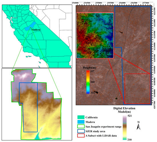
Figure 1.
An overview of the study area in the San Joaquin Experimental Range with false composite image and a subset with LiDAR data (right panel).
2.2. Data
2.2.1. LiDAR Data
Two airborne LiDAR datasets including DR LiDAR and FW LiDAR data were simultaneously collected through the National Ecological Observatory Network (NEON) Airborne Observation Platform (AOP) (Kampe et al., 2010) with an Optech Gemini instrument at a nominal range of 1000 m (the aircraft flew at 1000 m above ground level). FW LiDAR data acquired with this platform generated a 0.8 m diameter footprint, a spacing of about 0.524 m in the across-track direction and 0.5 m in the along-track direction. DR LiDAR data for corresponding study regions were also collected with the average point density approximately 6 points/m2 (ppm2). Both data sets were acquired in June 2013 during the leaf on season. These data can be downloaded from NEON data Portal (http://data.neonscience.org/home) and detailed technical specifications of data can be found in the study of [24].
Our study area is covered by two perpendicular direction flight lines, with four and two flight lines in an east-west direction and a north-south direction, respectively. In total, the study region was covered by 40,000,812 FWs, and each waveform is composed of 500 time bins with 1 ns temporal resolution. The tail of each waveform is filled with zero values to keep the length of waveforms constant. In fact, the zero values in the waveform represent non-record values. In addition to the waveform information, the corresponding waveform reference geolocation information was also used in this study. Specifically, seven basic reference geolocation attributes are directly used to geo-transform the waveform data to the HPC. The seven items are the Easting of first return xr (m), the Northing of first return yr (m), the height of first return zr (m), dxr (m), dyr (m), dzr (m), and first return reference bin location tr (leading edge 50% point of the first return).
2.2.2. Reference Data
The field data were collected through the NEON AOP and the Terrestrial Instrument System (TIS) programs (NEON, 2018a). In sum, there were 13 plots and totally 345 individual trees and shrubs (≤3 m) in our study area. These plots were designed for the long-term plant, insect and soil measurements following the protocol of the NEON Terrestrial Observation System (Meier and Jones, 2014) and each plot is restricted to a region 20 × 20 m. For each field-measured tree, key vegetation structure variables such as tree locations (Easing and Northing), tree height, and average crown width were provided (http://data.neonscience.org/prototype-search).
2.3. Methods
To get a better overview of the HPC generation process and their potential applications, we summarized the major steps of this study as shown in Figure 2. A detailed description of these steps can be found in subsequent sections.
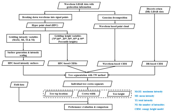
Figure 2.
The flowchart of utilizing the hyper point cloud to extract tree attributes.
2.3.1. From Raw Waveforms to Hyper Point Cloud
The routine for extracting FW LiDAR information is to convert part of waveform signals to discrete points with the decomposition or deconvolution methods, which has been proven useful for tree species identification, forest inventory, and biomass estimation [12,14,18,28]. However, most of the intensity information inherent in waveforms is ignored with the conventional methods, which undoubtedly degrades the value of FW LiDAR data. Moreover, the complicated waveform processing steps perplex users and further hinder the extensive use of FW LiDAR data for vegetation characterization. To tackle these challenges, we directly convert all raw waveform signals into points to form a point cloud, named the HPC, for subsequent analysis. A HPC is a set of data points converted from all waveform signals along the pulse path by combing waveform reference geolocation information (black) with raw waveform data (blue) (Figure 3).
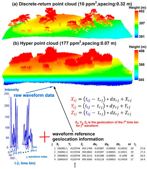
Figure 3.
Comparison of the discrete-return LiDAR point cloud and the hyper point cloud (HPC) over the same subset region. (a) Discrete-return LiDAR point cloud. (b) Illustration of the HPC generation process by combing raw waveform data (blue) and corresponding waveform reference geolocation information (black).
Specifically, we geo-transformed every time bin of the waveform into a point Pij = (Xij, Yij, Zij, Iij) (i = 1, …, nj, j = 1, …, m) through Equation (1) based on the whole return waveform signals and corresponding geo-reference data. Here, Iij is the intensity of the ith time bin for the jth waveform.
where , , is the geolocation of Iij, is the first return reference bin location for the jth waveform, , , are the position change for every nanosecond for the jth waveform, , are the Easting, Northing and height of the first return for the jth waveform. , , , are provided by the NEON geolocation dataset. Subsequently, we explored the potential of FW LiDAR data to characterize vegetation structure using the HPC.
2.3.2. Gridding of the Hyper Point Cloud
The HPC preserves as much information embed in original waveforms as possible and provides a convenient way to handle FW LiDAR data for most potential users. However, the large data volume of the HPC precludes its direct use for measuring vegetation structure. Additionally, not all signals converted from waveforms are useful for the subsequent analysis. Thus, we propose applying a grid-net method for the HPC to reduce the data volume and generalize the useful information it contains on the 3D vegetation structure.
In this study, we first explored the intensity variation in grid cells with different sizes to investigate the capability of waveform intensity information for segmenting tree objects and the spatial pattern of waveform intensity across various objects. Specifically, we projected the HPC’s intensities into XY planes to obtain the spatial distribution of energy with self-defined grid sizes. As shown in Figure 4, we directly applied a gridding process to the HPC and generated multiple grid-level variables such as the mean location of all intensities (Xc and Yc), the maximum intensity (MAXI), the mean intensity (MI), the total intensity of waveforms (TI) and the number of intensities (NI) for each grid. To find the appropriate grid size (based on the HPC density), multiple grid cell sizes, including 0.5 m, 0.8 m, 1 m, 1.5 m, 2 m, 3 m, 4 m and 5 m, were used. In addition to height information, PHs such as the 75th, 80th, 85th, 90th, 95th and 99th in each grid were also generated. At the current stage, we reduced the HPC to a manageable degree at grid level with various intensity and height metrics.
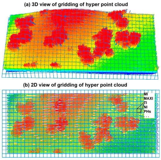
Figure 4.
The gridding of the hyper point cloud (HPC). (a) 3D view of the HPC with grid-nets. (b) Derivation of variables such as the mean intensity (MI), the maximum intensity (MAXI), the total intensity (TI), the number of intensities (NI) and multiple percentile heights (PHs) at the grid cell level with the gridding procedure from the 2D perspective.
2.3.3. The Intensity and Height Surfaces
To further investigate the intensity distribution of vegetation and ground objects at the local level, we assumed these variables such as the MI, MAXI and PHs were Z values like the height information of DR LiDAR data. Subsequently, we converted Xc, Yc and one of these variables to the point cloud as the LiDAR data exchange binary format (LAS) and generated the digital surface model (DSM) for each point cloud using the lasgrid function from LAStools [29]. Figure 5 exhibits an overview of preliminary results of digital surface model (DSM) form DR LiDAR data and the HPC with representative variables such as the MAXI, MI and 99th PH.
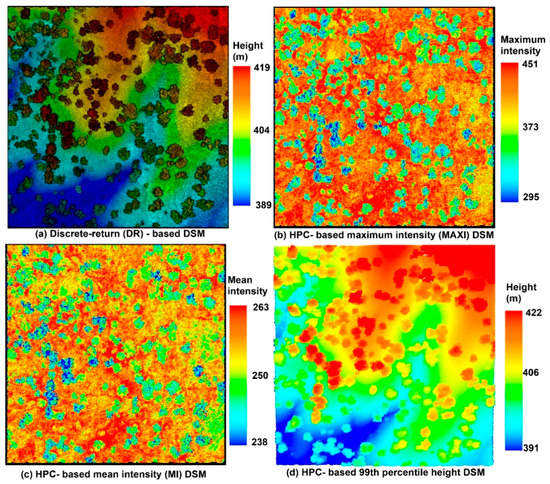
Figure 5.
Preliminary results of (a) the discrete-return (DR)-based digital surface model (DSM) and (b) the HPC-based MAXI DSM, (c) HPC-based MI DSM, and (d) HPC-based 99th percentile height (PH) DSM from the hyper point cloud (HPC).
It was evident that the HPC-based MAXI DSM, MI DSM and 99th PH DSM shared a similar spatial pattern with the DR-based DSM, which motivates us to further generate a surface analogous to the CHM surface. However, the HPC-based TI and NI DSMs did not provide as meaningful a spatial distribution as the HPC-based MAXI and MI DSMs based on the visual inspection. Thus, we did not carry out any further exploration of these two products for tree crown segmentation analysis in this study.
For visual analysis and semantic extraction of canopy information, a multi-level rescaling process was conducted on intensity-DSMs to generate CHM-like surfaces as shown in Figure 6. Specifically, the signs of values for the HPC-based intensity DSMs such as MAXI DSM and MI DSM were reversed to enable intensities over the vegetation higher than the ground region (Figure 6b). Subsequently, the absolute mean value of ground samples was added to these reversed intensities to generate positive intensity values for vegetation regions and negative values for the ground regions (Figure 6c). These negative values were reassigned to zero (Figure 6d). Furthermore, we rescaled the intensities to provide a more intuitive CHM-like surface (Figure 6e). To mitigate the effect of gaps on the surface, a smooth process was conducted to generate the no-gap surface as shown in Figure 6f, named it the HPC-based MAXI surface in the following sections.
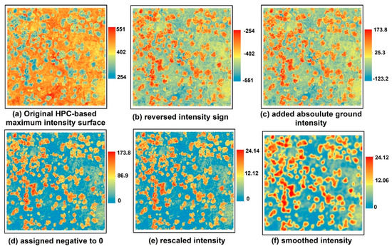
Figure 6.
An example of rescaling original HPC-based maximum intensity surface to generate a CHM-like surface.
For the HPC-based PH point clouds, we treated them as DR LiDAR data and generated the HPC-based PH CHM following the steps we described in previous studies [8,24]. Specifically, we first classified these HPC-based percentile heights point cloud into ground and non-ground categories using lasground function and then applied las2dem, lasgrid and lasmerge functions for these non-ground points to obtain the CHM. Simultaneously, the same procedures were applied to the DR LiDAR data and the waveform-based point cloud from the Gaussian decomposition [24] to generate DR-based CHM and waveform-based CHM.
2.3.4. Tree Crown Delineation
Tree crown segmentation is a preliminary and pivotal step for extracting and estimating individual tree attributes such as crown width and tree volume over large areas. Generally, the tree crown segmentation was conducted on the CHM derived from DR or FW LiDAR point cloud. In this study, we aim mainly to directly employ the HPC-based surfaces such as the MAXI intensity surface and PH CHMs to segment tree crowns and compare their results with conventional surfaces such as the DR-based and waveform-based CHMs.
Specifically, the tree crown segmentation was conducted on the DR and waveform-based CHMs, the HPC-based MAXI surface and HPC-based PH CHMs with the TW (the combination of TreeVaW and watershed algorithms) method [28]. First, the TW method adopted an adaptive variable window filtering approach [30] to identify tree tops using the local maxima algorithm. The core of the adaptive window filtering is that the size of the moving window varied with the height based on an empirical equation of the field-measured crown width (CW) and tree height (H). After the rescaling process, the HPC-based MAXI surface had a similar intensity range with the height range of CHMs, which enabled us to use the same empirical equations to initiate the tree top identification process. The minimum height (MINH) was the threshold used to filter ground for both CHMs and HPC-based intensity surface, while the MINH became the rescaled intensity instead of the height for the HPC-based intensity surface. The MINH was determined by averaging the heights or rescaled intensities from group samples in terms of visual inspection. To obtain reasonable tree top results, we refined the parameters with a trial and error method, with the ultimate parameters we used in this study summarized in Table 1. However, there is a distinct difference in the MINH between the LiDAR derived CHMs and the HPC-based MAXI surface. The main reason may be that the HPC-based MAXI surface stored relative intensity information rather than height information.

Table 1.
Key parameters for tree crown segmentation using the LiDAR derived CHMs, the HPC-based MAXI surface and percentile height CHMs (m).
As a further step, we followed the procedure described by Zhou et al. [28] to tackle the over-segmentation problem and acquire the adjusted tree top locations for the whole study. For each adjusted tree top, a tree crown was delineated using the marker-control watershed segmentation algorithm [31]. The tree location and tree crown results from the above step were compared with results from LiDAR derived CHMs and field-measured data to evaluate the performance of tree crown segmentation using the HPC-based MAXI surface and the HPC-based PH CHMs.
2.3.5. Individual Tree Intensity Distribution
Besides the exploration of FW LiDAR data at the local level in Section 2.3.4, we also investigated the intensity distribution of FW LiDAR data at individual tree level. Specifically, we employed the individual tree crowns obtained from the above step to subset the HPC and obtained individual trees’ HPCs. Subsequently, we applied a 0.8 m (the footprint diameter is approximately 0.8 m) grid-net described above to these individual HPCs and obtained corresponding grid statistics or variables such as the MI, MAXI, TI and NI (Figure 4). Three representative tree segments were chosen to demonstrate the intensity or energy distribution of individual trees in the contour line format.
2.3.6. Individual Tree Attributes
We next explored potential applications of the HPC-based surfaces for identifying tree top location, and estimating tree crown width and tree height using the delineated tree crowns and the HPC. Briefly, the tree top location in each delineated crown was identified as the MAXI’s location through the local maximal algorithm; the crown width was calculated as the diameter of each individual delineated tree crown by assuming that the tree crown was circular. To quantitatively assess the HPC-based MAXI surface and the HPC-based PH CHMs’ capacity for measuring these tree attributes, we computed the mean difference (MD) between the estimated attributes and the field-measured data, their corresponding standard deviation (SD) and root mean square error (RMSE). Additionally, the percentage of estimated tree locations within the 2.5 m buffer of field-measured tree locations (Pdis<2.5) was also calculated.
For the tree height estimation, we directly derived tree height from the CHMs (the DR-based, waveform-based and HPC-based PH) by obtaining the maximum value within a 2.5 m circle around each estimated tree location. However, the HPC-based MAXI surface only stored intensity information which was not directly relevant to tree height and required additional steps for estimating tree height from it. We considered two methods to extract tree height from fine resolution HPC-based MAXI surface alone: (1) building a linear relationship between intensity variables and heights using the training data (70% of all reference data) and applying this relationship to the testing data (30% of all reference data) to assess the performance of tree height estimation. The simple linear relationship used here was mainly to ensure the model’s generality and transferability. The intensity variables were extracted from 2.5 m circle buffers initiated from the identified tree locations and calculated the minimum, maximum, mean and total intensities in each buffer as variables; (2) combing tree top locations derived from the HPC-based MAXI surface with the HPC to estimate tree height through filtering procedures using intensity and height information. The assumption of this approach is that the ground and tree top correspond to the points whose intensities are around the MAXI of each estimated tree crown. More specifically, we first selected points within a circle of estimated tree top locations to obtain possible ground and top of the canopy points. The range of radius for the circle was determined with a trial-and-error approach that worked efficiently in our study site was 2–3 m. Next, these points whose intensity falling into the intensity range [MAXI − ratio * MAXI, MAXI + ratio * MAXI] were assumed to contain useful ground and tree height information as the filtered point cloud. Here, the MAXI represents the maximum intensity in the selected points in each circle. We achieve robust estimates when the ratio was within [0.02, 0.06]. Furthermore, the tree height was calculated as the average of difference between the tree top PH (97th, 98th, 99th) and ground PH (1st, 2nd, 3rd) of the filtered point cloud. These percentiles were mainly to avoid the negative effect of outliers and were determined based on the experiment of multiple adjacent ranges of percentiles. Additionally, multiple percentiles can mitigate the error caused by practical factors such as various terrain conditions and irregular tree structures. The effectiveness of this method was evaluated by comparing estimated tree height with corresponding field data.
3. Results
3.1. Hyper Point Cloud
The comparison between the DR LiDAR point cloud and the HPC over a small subset region is presented in Figure 3. Overall, the HPC was consistent with the DR point cloud to some extent in terms of the spatial arrangements of ground and vegetation. However, the HPC of a subset region was much denser than DR LiDAR point cloud with the point density, approximately 177 vs. 10 ppm2, and the average spacing among points was 0.07 vs. 0.32 m. As shown in Figure 3, more signals were over the top of the canopy and beneath the ground, which consequently contributed to larger ranges of height for the HPC. A closer examination revealed that the mid-story of vegetation for the HPC was also filled with signals. In contrast, most of the mid-story height levels of vegetation were empty for the DR point cloud. Nevertheless, the HPC did not present as explicit vegetation object shapes as the DR LiDAR point cloud. In sum, the HPC provides a new way to visualize FW LiDAR data and preserve a wealth of information inherent in FW LiDAR data with promising potentials for characterizing vegetation structure.
3.2. HPC-Based Intensity and Height Surfaces
Figure 5 illustrates the HPC-based intensity and PH DSMs with the LiDAR-derived DSM. Overall, these DSMs shared similar patterns with consistent spatial arrangements of vegetation and ground. For the HPC-based intensity DSMs, the vegetation parts (blue) are prone to have lower MAXI and MI values compared to the ground parts (red). The HPC-based PH DSM was almost identical to the DR-based DSM except for the height range. More specifically, the HPC-based PH DSM was consistently higher than DR-based DSM, at approximately 3 m.
To further demonstrate the potential usefulness of these products, we generated a CHM-like surface with multi-level rescaling steps. As an example, Figure 6 shows the detailed steps of rescaling the HPC-based MAXI surface over a subset region to elaborate on the usefulness of these steps. These steps are mainly intended to generate representative intensity information for distinguishing the vegetation and ground with the simple linear conversion.
The comparisons between these two HPC-based intensity surfaces (the MAXI and MI) and the HPC-based 99th PH CHM are shown in Figure 7. As expected, the HPC-based intensity surfaces exhibited a spatial pattern similar to CHMs after multi-level rescaling; the higher rescaled intensities corresponded to vegetation areas with high CHM values and smaller rescaled intensities were located on the ground with low CHM values. However, the height variance (the CHM) for vegetation was larger than the corresponding region’s rescaled intensity variance (the HPC-based intensity surfaces) with more homogenous intensity (red) (Figure 7c,d). Regarding the ground areas, more variations of the rescaled intensity for the HP-based intensity surfaces were observed compared to these CHMs, especially when the HPC-based MI surface was taken into account (Figure 7d). Interestingly, we found some “mixed” areas that could be classified as either ground or vegetation in both HPC-based intensity surfaces, as depicted with blue circles, while they were deemed to be the ground in the CHMs (Figure 7a,b) with low heights. Moreover, the HPC-based MI surface appeared to generate more “mixed” areas than the HPC-based MAXI surface, which gave rise to the problematic tree crown segmentation in the later stage. Therefore, the HPC-based MAXI surface might hold greater potential for characterizing vegetation and ground. For the HPC-based PH surfaces, the 99th PH CHM was prone to better captured the vegetation than 95th PH CHM with closer height values and less “noise” parts compared to the DR-based CHM.
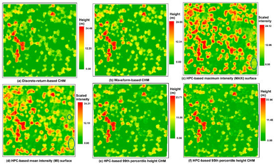
Figure 7.
Comparisons of the (a) DR-based CHM, (b) waveform-based CHM, (c) HPC-based maximum intensity (MAXI) surface, (d) HPC-based mean intensity (MAXI) surface, (e) HPC-based 99th PH CHM, and (f) HPC-based 95th PH CHM over a subset region.
3.3. Individual Tree Intensity Distribution
Beyond the local level, the energy (intensity) distributions of FW LiDAR data at the individual tree level were also examined, and three representative individual trees were selected as examples to demonstrate the spatial energy distribution patterns at the individual tree level. To get an overview of DR LiDAR point cloud and the HPC at individual tree level, we present them in Figure 8 with four intensity distributions of these trees in a contour line format. It was evident that the HPC was denser than DR LiDAR data, especially at the mid-story height levels of trees. Regarding the intensity distribution, these four intensity variables followed the anisotropic distribution, whether within one tree or across different trees (Figure 8). However, some consistent spatial distribution patterns were observed across different trees. For example, the individual trees’ MAXI and MI contours demonstrated that the original intensity value was increasing from the center to the boundary of tree crown with the lowest value in the center of tree crown. Conversely, the contours of the TI and NI exhibited totally opposite changing pattern, decreasing from the center to the boundary of tree crown, with the highest values at the center of tree crown. These individual tree level contours provided valuable insight into the potential of the HPC-based intensity surfaces for identifying tree top locations and delineating tree crowns.
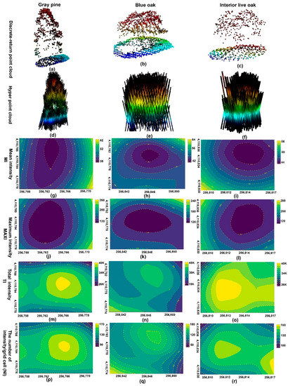
Figure 8.
First row: Discrete-return point cloud of three representative individual trees including the (a) gray pine, (b) blue oak and (c) interior live oak. Second row: The HPC of three individual trees (d), (e,f). Third row: The energy distributions of three representative individual trees (g–i) using mean intensity (MI). Fourth row: The energy distribution of three representative individual trees (j–l) using maximum intensity (MAXI); Fifth row: The energy distribution of three representative individual trees (m–o) using total intensity (TI). Sixth row: The energy distribution of three representative individual trees (p–r) using the number of intensity/grid cell (NI) (0.8 m). K: 1000.
3.4. Potential Applications
3.4.1. Tree Crown Delineation
Preliminary results of tree crown segmentation demonstrated that the HPC-based MAXI surface was superior to the MI surface for delineating tree crowns. One possible reason is that the MAXI is more likely to represent the top of canopy while the MI considered both the top and understory layers. The tree crown delineation relied more on the tree top surface. Thus, the subsequent tree attributes analysis was only conducted on the HPC-based MAXI surface. Various grid cell sizes affected performances of tree crown delineation using the HPC-based MAXI surface. As shown in Figure 9, several representative crown delineation results of HPC-based MAXI surfaces (black) and HPC-based PH CHMs’ (blue) are presented as compared to the DR-based, waveform-based CHMs (red). Based on visual inspection, there are no significant differences among tree crown segmentation results.
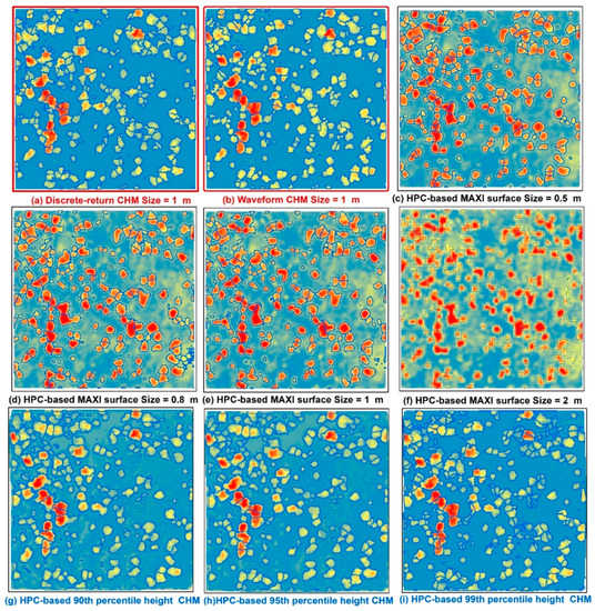
Figure 9.
Tree crown segmentation results using (a) discrete-return, (b) waveform-based CHMs (red), HPC-based intensity surfaces with different grid cell sizes (c) 0.5 m, (d) 0.8 m, (e) 1 m, and (f) 2 m (black), (g) HPC-based 90th PH, (h) 95th PH, and (i) 99th PH CHM (blue) over the subset region.
To further quantitatively assess the tree crown delineation results, Table 2 summarizes vegetation area, ratio of vegetation areas, and tree crown detection rate for both CHMs and WISs after being compared to reference data. As illustrated in the visual comparisons, the HPC-based MAXI surfaces with the fine grid cell sizes such as 0.5, 0.8 and 1 m can give comparable results as the LiDAR-derived CHMs with overall tree crown detection rate centering on 90%. However, results of tree crown detection rate significantly decrease when the grid cell size became larger than 1 m.
Table 2.
Summary statistics of comparisons among the DR-based CHM (DR-CHM), waveform-based CHM (waveform-CHM) and the HPC-based MAXI (HPC-MAXI) and the HPC-based percentile height (HPC-PH) surfaces over the study area.
Overall, visual comparisons of tree crown segmentation results between CHMs and the HPC-based MAXI surfaces (Figure 9c–f) reveal consistently satisfactory segmentation results, but the HPC-based MAXI surfaces are prone to generate additional tree crowns at “mixed” regions (red circle).
3.4.2. Individual Tree Attributes
We further assessed the accuracy of tree attributes extracted from the HPC-based MAXI surface and PH CHMs such as the crown width, tree top location and tree height. Overall, the HPC-based MAXI surface (≤1 m) and PH CHMs generated comparable estimates of the crown width, tree top location and tree height compared to the LiDAR derived CHMs in terms of MD, SD, RMSE and Pdis<2.5. Nevertheless, the crown width estimation results demonstrated that the HPC-based MAXI surfaces with fine resolution (≤1 m) yielded more accurate estimates than the LiDAR derived CHMs (e.g., RMSEHPC-MAXI0.5 = 2.39 vs. RMSEDR = 3.69 m) (Table 2). In contrast, tree top locations were better captured by the LiDAR-derived CHMs than the HPC-based MAXI surface from the perspective of the MD and RMSE. Among the HPC-based MAXI surfaces, coarse resolution surfaces were prone to give less accurate estimates and the HPC-MAXI0.5 outperformed other HPC-based intensity surfaces in terms of the crown width and tree location estimation results. Although the HPC-based PH DSMs appeared to be shifted form DR-based DSM, the various HPC-based PH CHMs demonstrated a promising estimation of crown width and tree location comparable to the LiDAR-derived CHMs with all RMSE values smaller than 3 m.
Regarding the tree height estimation, the HPC-based PH CHM almost yielded the same results as the LiDAR derived CHMs, especially for the 99th PH CHM (Table 3). Given that the HPC-based MAXI surface did not directly store height information like the CHMs, we proposed two methods to extract height information. Results of the first method using a linear relationship between height and rescaled intensity are demonstrated in Figure 10. A general trend emerges from this figure that higher heights are more likely to have higher rescaled intensities. However, there is a weak relationship between rescaled intensities and reference height with low R-square but acceptable RMSE (~2.5 m). Moreover, there is no significant difference among the use of minimum, maximum, mean and total rescaled intensities of the buffer to estimate tree height.
Table 3.
Tree height estimation using DR-based CHM, waveform-based CHM, the HPC-based MAXI surfaces with the first method (HPC-MAXI0.5_first & HPC-MAXI0.8_first) and the second method (HPC-MAXI0.5_s (before adjustment), HPC-MAXI0.5_s (after adjustment), HPC-MAXI0.8_s (before adjustment) & HPC-MAXI0.8_s (after adjustment)) and HPC-based PH (99th, 95th, 90th) CHMs.
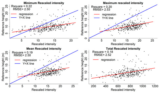
Figure 10.
The linear relationship between reference tree height and mean rescaled intensity (minimum, maximum, mean and total rescaled intensities) within the 2.5 m buffer of the waveform intensity surface (WIS, 0.5 m resolution).
For the second method, we obtained robust estimates of tree height using various tree top and ground percentiles with appropriate radius and filtering intensity ranges. The various tree top and ground percentiles used here were mainly intended to leverage the bias of the estimate. Our experiment showed that the choice of radius has a larger impact than the intensity range for accurately estimating tree height from the HPC. The suitable range for the radius is [2, 3] m, and the ratio of intensity range is [0.03, 0.06] according to our experiment. The preliminary results (before adjustment) of the second method indicated that tree height was overestimated consistently by approximately 1 m from the HPC-based MAXI surface (Figure 11a). After subtracting 1 m from original estimated heights, we obtained a smaller average bias (−1.10 vs. −0.10 m) and RMSE (1.78 vs. 1.40 m) of differences between the estimated tree height and reference tree height (Figure 11). In terms of the MD and RMSE, the second method outperformed the first method for estimating height information from the HPC-based MAXI surface. However, the height estimation results from the HPC-based MAXI surface did not generate as good results as the HPC-based PH CHMs. Among various PHs, the 99th HPC-based PH CHM gives the best height estimation result. Interestingly, all height estimation from FW LiDAR data, including waveform-based and HPC-based products, overestimated the tree height, with MD of less than zero, while DR LiDAR data underestimated the tree height.
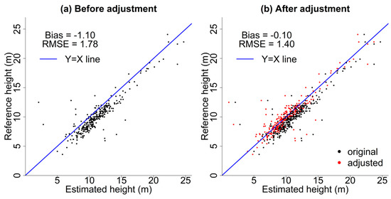
Figure 11.
The comparisons between (a) original height estimation from the HPC-based MAXI surface and (b) adjusted height estimation with simple subtraction refine process using the radius = 3 m and intensity range = 0.05.
4. Discussion
The emphasis of this study was on expanding the potential uses of FW LiDAR data from a new perspective and enhancing their value for vegetation characterization. We introduced the HPC and HPC-based products or concepts by directly using FW LiDAR data without complicated processing algorithms, and exemplified their uses for characterizing vegetation structure.
4.1. Hyper Point Cloud
A plethora of information inherent in FW LiDAR data is stored in the wave format, which cannot be easily processed by most practitioners to extract useful vegetation biophysical parameters. We proposed an approach to directly convert waveform data into a point cloud with a structure that is well known to remote sensing and ecological scientists. To some extent, this will alleviate the difficulty we experienced in understanding and employing sophisticated algorithms for extracting information from FW LiDAR data [24,25]. Moreover, our approach also provides a competitive alternative way to the conventional method for processing FW LiDAR data. Previous studies have explored potential uses of FW LiDAR for vegetation characterization such as tree species identification and global canopy height mapping using features extracted from waveforms [15,28]. However, some amount of raw information will automatically be lost during these existing procedures. With the advent of the HPC, all original information contained in FW LiDAR data is preserved by converting every signal of the waveforms into a point. However, the shape of the waveforms cannot be directly obtained, as with the Gaussian decomposition method, which can interpret the shape of waveforms through the estimated echo widths and amplitudes.
Additionally, how to directly visualize complete FW LiDAR data over a region like DR LiDAR data is still an open question that challenges the remote sensing community. The HPC provides a solution to this question and enables users to straightforwardly visualize FW LiDAR data using available handy tools designed for DR LiDAR data, as shown over a subset region (Figure 3) and individual trees (Figure 8). This point cloud is analogous in format to terrestrial LiDAR data, to some extent, with detailed information in the mid-story of the canopy. As anticipated, the HPC is approximately 18 times or more, on average (varies on the overlap of flight lines), denser than corresponding DR LiDAR data by keeping all signal intensities along the pulse path. It is worth noting that the vegetation or canopy parts of the HPC are composed of a substantial number of points instead of sparsely sampling points from the top of the canopy for the DR LiDAR point cloud (Figure 8). This could overcome the disadvantage of airborne DR LiDAR data that cannot provide detailed information in the mid-story of vegetation. Meanwhile, it also leaves us considerable room and flexibility to exploit their potential applications such as semantic segmentation and vegetation structure reconstruction.
Overall, the HPC, with its point cloud format and the rich information it contains, gives interpreters or users more accessibility and flexibility to investigate the potentials of FW LiDAR data for multiple purposes. Certainly, the HPC requires more storage space and calls for more efforts to exploit and interpret the ample information inherent in waveforms. However, there is little doubt that the HPC can render new perspectives on investigating vegetation structure and facilitate extensive applications of FW LiDAR data with the continued technological advances.
4.2. HPC-Based Intensity and Height Surfaces
To enhance the practical value and use efficiency of the HPC, we exemplify a grid-based statistical method to generate the thinned version of point cloud for characterizing vegetation structure. The HPC-based intensity (MAXI and MI) DSMs exhibit promising prospects for distinguishing vegetation and ground as shown in Figure 5. Interestingly, higher MAXI and MI are more likely to present at the ground sections rather than vegetation sections. The vegetation has a complex porous structure, while the ground is an impenetrable surface. Consequently, more energy loss occurs during the process of the pulse passing through the gaps of vegetation layers compared to directly interacting with ground given the same amount of pulse energy. This is also substantiated by the fact that the first peak intensity of the waveform (amplitude) generally has larger values than the subsequent amplitudes [24]. However, the vegetation could give rise to more signal returns that result in higher TI and NI for a given region. Surprisingly, the spatial patterns of the HPC-based TI and NI DSMs are not as evident as the HPC-based MI and MAXI DSMs (Figure 5). A closer examination of these HPC-based intensity DSMs reveals that a different number of overlapping flight lines mainly contributed to this discrepancy. At this point, the vegetation and ground can be well captured by the HPC-based intensity products.
LiDAR-derived CHM is deemed as the most fundamental and valuable model to characterize vegetation parameters such as tree height, crown width and biomass for complementing forest inventory [14,30,32,33]. The motivation for rescaling the original intensity information is to generate a CHM-like product and further assess the feasibility of the HPC-based intensity surface for augmenting or substituting CHM in the study of forest structure and improve the accuracy of estimating individual tree attributes. To generalize the rescaling steps and preserve original intensity information inherent in the HPC, all steps are done with simple linear conversion. Among four representative HPC-based intensity surfaces, the HPC-based MAXI surface is more likely to give us a better separation of vegetation and ground. The possible reason for this is that the MAXIs (amplitude) of waveforms generally correspond to the objects such as trees and ground that the pulses interact with, and different objects give different amplitude values. For instance, the waveforms coming from ground sections yield similar maximum intensities, while they differ significantly from the maximum intensities from vegetation components, which results in the discernible boundary between ground and vegetation. Of particular note, multiple possible variables or features such as intensity percentiles can also be extracted from the HPC. We encourage researchers to further exploit other variables or features from the HPC to further test their utilities and validity over various types of forest.
As expected, the HPC-based PH CHMs demonstrate the promising prospects of the PHs as surrogates for canopy structure variables from the HPC. These CHMs show consistent or identical spatial distribution with the DR-based and waveform-based CHMs. Overall, the proposed approaches for obtaining the HPC-based intensity and height surface not only expand existing approaches for processing FW LiDAR data, but also provide a new insight into fully using FW LiDAR data for characterizing canopy structure.
4.3. Individual Tree Intensity Distribution
Along with the HPC-based intensity and height surface results, the detailed energy distribution at the individual tree level is also examined (Figure 8). The waveform intensity contours of three representative trees provide a theoretical justification for potential applications of the HPC-based surfaces. For instance, the most inner contour of an individual tree is more prone to be the tree top locations and the outer contour is similar to the shape of a tree crown boundary.
The intensity contours such as the MAXI, MI, TI and NI at the individual tree level provide insight into the changing pattern of energy over the vegetation at a high level of detail. Both the MAXI and MI contours reveal that the intensities are increasing from the center of tree crown to the boundary of the tree. This can be explained by the fact that more energy loss occurs during the penetration process over the center of tree crown with taller vegetation, where more dense vegetation is present, compared to the boundary of the tree in general [34]. As a consequence, smaller amplitudes or maximum intensities were returned from the region with dense vegetation. Analogous to the TI and NI WISs, the TI and NI contours at the individual tree level exhibit decreasing pattern from the center of tree crown to the boundary of the tree. More signal returns are generated from the center of tree crowns or dense vegetation areas can attribute to this pattern. Additionally, there is a pronounced difference of contour center and changing patterns between the MAXI and MI, and the TI and NI contours. These inconsistencies are possibly due to the TI and NI contours being obtained from more “noise” in the point clouds resulted from multiple flight lines compared to the MAXI and MI contours. In addition, the lack of calibration or proper normalization steps for the TI and NI products also potentially counteract their usefulness for subsequent tree analysis. Of course, the calibration of the MAXI and MI products is also needed to enhance their capability for vegetation characterization or extend new potential applications. However, it is beyond the scope of this study to investigate proper intensity calibration procedures. Our further research will aim to explore the proper calibration or normalization steps for efficiently using the HPC or the HPC-based surfaces.
Although we only examine these four variables for the HPC, there is little doubt that other variables or features extracted from the HPC will be useful as competitive alternatives for solving potential research problems, such as using contour boundaries or intensity percentiles to estimate fuel loads of forests, crown base height, or to better characterize the horizontal and vertical vegetation structure. Overall, the contours of intensity distribution at the individual tree level provide a theoretical justification to extract attributes from the HPC-based surfaces for characterizing tree structure and ultimately promote the extensive use of FW LiDAR data.
4.4. Potential Applications
The HPC-based intensity and height surfaces provide a new perspective for employing intensity information to characterize vegetation structure and exhibits the HPC’s potential usefulness, which is expected to spur more efforts to explore these products for practical and scientific applications. We exemplify the utility of these surfaces for delineating tree crowns, identifying tree top locations, estimating crown width and tree height in this study. These applications offer an alternative way to extract information from FW LiDAR data and boost the use of information inherent in waveforms.
Tree crown segmentation is the fundamental procedure for forest inventory and monitoring, which is commonly conducted on the LiDAR-derived CHM [13,28,31]. Our tree detection comparisons suggest that the fine resolution HPC-based MAXI surfaces can generate comparable results to the DR and waveform-based CHMs with the tree detection rates being around 90%. The accurate tree detection and crown segmentation results render promising prospects for subsequent tree attribute estimation. Our results also suggest that the HPC-based intensity surfaces with various resolution are prone to detect additional vegetation areas compared to the CHMs. As noted from the blue circles in Figure 7, the WISs appear to have some “noise” compared to CHMs, but a closer examination reveals that these regions are covered with low vegetation (<3 m) such as California sagebrush. This finding may shed light on detecting understory layers or studying savanna ecosystems using intensity information of FW LiDAR data [24]. Overall, the performance of the WIS’s tree crown segmentation is comparable to the CHM and demonstrate the potential of the HPC-based MAXI surface as an alternative product to the CHM for vegetation characterization.
Results of individual tree attributes estimated from the HPC-based intensity and height surfaces further confirmed the promising prospect of the HPC. Compared to the tree location identification and crown width estimation, the tree height estimation from the HPC-based MAXI surface is less direct and more challenging to derive than the CHMs. We developed two methods to explore the potential of tree height estimation directly from the HPC-based MAXI surface. The motivation of the first method was to examine whether a simple relationship between the height and normalized intensity exists. Despite the fact that a parsimonious linear relationship does not exist in this study (low R-square), a general trend between the height and normalized intensity is observed without the field-based intensity calibration step. Nevertheless, this method holds promise for enhancing the tree height predictive capability after conducting proper calibrations. Compared to the results of the first method, the second method can achieve better results through additional processing steps. We integrated the HPC-based MAXI surface with the HPC to search possible points containing ground and tree top through the criteria such as the radius around the estimated tree locations and intensity ranges of these points. Moreover, our results may be improved with other possible tree height estimation methods such as combing the tree locations identified by the HPC-based MAXI surface with the height from the HPC-based PH CHM. Ultimately, these potential applications of the WIS exhibit promising prospects of HPC and provide significant implications for measuring fine-scale vegetation attributes with intensity information. As anticipated, the HPC-based PH CHMs outperform the HPC-based MAXI surface for estimating tree height and generate similar tree height estimation to the DR and waveform-based CHMs in terms of the MD and RMSE.
To the best of our knowledge, the concepts or products of the HPC, the HPC-based intensity and height surfaces are new to remote sensing and ecological communities. It is anticipated that these new concepts and products can pave a new way to make the most use of waveform intensity information, facilitate extensive use of FW LiDAR data and expand their promising applications for characterizing vegetation structure. A wealth of original information is contained in the HPC, but practical applications such as biomass estimation or fuel load assessment require us to identify representative and critical variables or features. We hope our potential application examples could encourage more efforts to recognize and draw out significant information from the HPC for characterizing vegetation structure. Moreover, there are also opportunities to advance the understanding the energy or radiative transfer modeling of vegetation through integrating optical earth observations with these products. Certainly, careful calibration of the intensity is needed to ensure the consistent performance or accuracy of models. Overall, the HPC and the HPC-based intensity and height surfaces presented in this study represent a new means for studying vegetation structure using FW LiDAR data and offer promising prospects for serving different user groups with a deep understanding of waveform intensity and height information.
5. Conclusions
Conventional ways of extracting FW LiDAR information, such as using the decomposition or waveform signatures, require sophisticated algorithms and deep understanding of waveform data, which curbs the widespread use of FW LiDAR data and further obstruct their potential and extensive applications for vegetation characterization. The HPC proposed in this study not only presents a direct way to visualize FW LiDAR data with available software, but also mitigates the technical barriers for most potential practitioners and further enables FW LiDAR data processing to become more accessible to remote sensing and ecological communities. Simultaneously, this product preserves as much information of raw FW LiDAR data as possible, offering users more flexibility to interpret and decode the information inherent in waveforms. The HPC-based intensity and height surfaces exemplify the potential applications of the HPC. These applications not only expand existing ways or products for vegetation characterization but may also provide an exciting new direction for vegetation structure characterization using intensity information of FW LiDAR data. The intensity distribution of vegetation at the tree level with contours provide the theoretical justification for subsequent individual tree analysis using the HPC-based MAXI surfaces. Individual tree attribute analysis, such as tree location identification, crown width and tree height estimation, provide initial proofs for the usefulness of the HPC and the HPC-based intensity and height surfaces from the practical perspective rather than just a conceptual approach. Despite that the HPC-based MAXI surface can achieve comparable or better results compared to the CHMs in some aspects, we made no attempt to substitute the CHM with the HPC-based MAXI surface but instead to complement each other for accurately characterizing vegetation structure using both height and intensity information. Given the high density and mid-story detection capacity of the HPC, it is feasible to analyze the detailed internal structure of individual trees or vegetation over a large region. Additionally, the contours of individual trees’ intensity distributions also provide insights into other potential applications, such as estimating the crown base heights and forest surface fuel load or even identifying tree species. Actually, the HPC-based intensity and height surfaces provides promising prospects in the 2D perspective, further research is also needed to develop approaches to obtain vegetation structure or biophysical attributes with detailed 3D reconstruction models using FW LiDAR data.
Author Contributions
T.Z. designed and conceptualized approaches to generate the HPC. S.P. provided guidance and feedback on methods and result demonstration. L.M. and K.Z. gave feedback and comments on the manuscript. K.K. provided reference data. All authors contributed to the editing of the manuscript.
Funding
This research was funded by the NSF Doctoral Dissertation Improvement Grant (DEB1702008) and NASA’s ICESat-2 SDT (Grant # NNX15AD02G).
Acknowledgments
We would like to thank the National Ecological Observatory Network (NEON) for providing waveform LiDAR and field data. Additionally, we greatly appreciate the constructive comments from two anonymous reviewers.
Conflicts of Interest
The authors declare no conflicts of interest.
References
- Falkowski, M.J.; Evans, J.S.; Martinuzzi, S.; Gessler, P.E.; Hudak, A.T. Characterizing forest succession with lidar data: An evaluation for the Inland Northwest, USA. Remote Sens. Environ. 2009, 113, 946–956. [Google Scholar] [CrossRef]
- Zhao, K.; Popescu, S.; Nelson, R. Lidar remote sensing of forest biomass: A scale-invariant estimation approach using airborne lasers. Remote Sens. Environ. 2009, 113, 182–196. [Google Scholar] [CrossRef]
- Dubayah, R.; Sheldon, S.; Clark, D.; Hofton, M.; Blair, J.; Hurtt, G.; Chazdon, R. Estimation of tropical forest height and biomass dynamics using lidar remote sensing at La Selva, Costa Rica. J. Geophys. Res. Biogeosci. 2010, 115. [Google Scholar] [CrossRef]
- Mallet, C.; Bretar, F. Full-waveform topographic lidar: State-of-the-art. ISPRS J. Photogramm. Remote Sens. 2009, 64, 1–16. [Google Scholar] [CrossRef]
- Chauve, A.; Vega, C.; Durrieu, S.; Bretar, F.; Allouis, T.; Pierrot Deseilligny, M.; Puech, W. Advanced full-waveform lidar data echo detection: Assessing quality of derived terrain and tree height models in an alpine coniferous forest. Int. J. Remote Sens. 2009, 30, 5211–5228. [Google Scholar] [CrossRef]
- Drake, J.B.; Dubayah, R.O.; Clark, D.B.; Knox, R.G.; Blair, J.B.; Hofton, M.A.; Chazdon, R.L.; Weishampel, J.F.; Prince, S. Estimation of tropical forest structural characteristics using large-footprint lidar. Remote Sens. Environ. 2002, 79, 305–319. [Google Scholar] [CrossRef]
- Wagner, W.; Hollaus, M.; Briese, C.; Ducic, V. 3D vegetation mapping using small-footprint full-waveform airborne laser scanners. Int. J. Remote Sens. 2008, 29, 1433–1452. [Google Scholar] [CrossRef]
- Zhou, T.; Popescu, S.C. Bayesian decomposition of full waveform LiDAR data with uncertainty analysis. Remote Sens. Environ. 2017, 200, 43–62. [Google Scholar] [CrossRef]
- Reitberger, J.; Krzystek, P.; Stilla, U. Analysis of full waveform LIDAR data for the classification of deciduous and coniferous trees. Int. J. Remote Sens. 2008, 29, 1407–1431. [Google Scholar] [CrossRef]
- Hancock, S.; Anderson, K.; Disney, M.; Gaston, K.J. Measurement of fine-spatial-resolution 3D vegetation structure with airborne waveform lidar: Calibration and validation with voxelised terrestrial lidar. Remote Sens. Environ. 2017, 188, 37–50. [Google Scholar] [CrossRef]
- McGlinchy, J.; van Aardt, J.A.N.; Erasmus, B.; Asner, G.P.; Mathieu, R.; Wessels, K.; Knapp, D.; Kennedy-Bowdoin, T.; Rhody, H.; Kerekes, J.P.; et al. Extracting Structural Vegetation Components From Small-Footprint Waveform Lidar for Biomass Estimation in Savanna Ecosystems. IEEE J. Sel. Top. Appl. Earth Obs. Remote Sens. 2014, 7, 480–490. [Google Scholar] [CrossRef]
- Cao, L.; Coops, N.; Hermosilla, T.; Innes, J.; Dai, J.; She, G. Using Small-Footprint Discrete and Full-Waveform Airborne LiDAR Metrics to Estimate Total Biomass and Biomass Components in Subtropical Forests. Remote Sens. 2014, 6, 7110–7135. [Google Scholar] [CrossRef]
- Reitberger, J.; Schnörr, C.; Krzystek, P.; Stilla, U. 3D segmentation of single trees exploiting full waveform LIDAR data. ISPRS J. Photogramm. Remote Sens. 2009, 64, 561–574. [Google Scholar] [CrossRef]
- Allouis, T.; Durrieu, S.; Véga, C.; Couteron, P. Stem volume and above-ground biomass estimation of individual pine trees from LiDAR data: Contribution of full-waveform signals. IEEE J. Sel. Top. Appl. Earth Obs. Remote Sens. 2013, 6, 924–934. [Google Scholar] [CrossRef]
- Lefsky, M.A.; Harding, D.J.; Keller, M.; Cohen, W.B.; Carabajal, C.C.; Del Bom Espirito-Santo, F.; Hunter, M.O.; de Oliveira, R. Estimates of forest canopy height and aboveground biomass using ICESat. Geophys. Res. Lett. 2005, 32, L22S02. [Google Scholar] [CrossRef]
- Harding, D.J.; Carabajal, C.C. ICESat waveform measurements of within-footprint topographic relief and vegetation vertical structure. Geophys. Res. Lett. 2005, 32, L21S10. [Google Scholar] [CrossRef]
- Anderson, K.; Hancock, S.; Disney, M.; Gaston, K.J.; Rocchini, D.; Boyd, D. Is waveform worth it? A comparison of LiDAR approaches for vegetation and landscape characterization. Remote Sens. Ecol. Conserv. 2016, 2, 5–15. [Google Scholar] [CrossRef]
- Yao, W.; Krzystek, P.; Heurich, M. Tree species classification and estimation of stem volume and DBH based on single tree extraction by exploiting airborne full-waveform LiDAR data. Remote Sens. Environ. 2012, 123, 368–380. [Google Scholar] [CrossRef]
- Hermosilla, T.; Ruiz, L.A.; Kazakova, A.N.; Coops, N.C.; Moskal, L.M. Estimation of forest structure and canopy fuel parameters from small-footprint full-waveform LiDAR data. Int. J. Wildland Fire 2014, 23, 224. [Google Scholar] [CrossRef]
- Wang, H.; Glennie, C. Fusion of waveform LiDAR data and hyperspectral imagery for land cover classification. ISPRS J. Photogramm. Remote Sens. 2015, 108, 1–11. [Google Scholar] [CrossRef]
- Finley, A.O.; Banerjee, S.; Cook, B.D.; Bradford, J.B. Hierarchical Bayesian spatial models for predicting multiple forest variables using waveform LiDAR, hyperspectral imagery, and large inventory datasets. Int. J. Appl. Earth Obs. Geoinf. 2013, 22, 147–160. [Google Scholar] [CrossRef]
- Babcock, C.; Finley, A.O.; Cook, B.D.; Weiskittel, A.; Woodall, C.W. Modeling forest biomass and growth: Coupling long-term inventory and LiDAR data. Remote Sens. Environ. 2016, 182, 1–12. [Google Scholar] [CrossRef]
- Wang, H.; Glennie, C.; Prasad, S. Voxelization of full waveform LiDAR data for fusion with hyperspectral imagery. In Proceedings of the 2013 IEEE International on Geoscience and Remote Sensing Symposium (IGARSS), Melbourne, VIC, Australia, 21–26 July 2013; pp. 3407–3410. [Google Scholar]
- Zhou, T.; Popescu, S.C.; Krause, K.; Sheridan, R.D.; Putman, E. Gold—A novel deconvolution algorithm with optimization for waveform LiDAR processing. ISPRS J. Photogramm. Remote Sens. 2017, 129, 131–150. [Google Scholar] [CrossRef]
- Wu, J.; van Aardt, J.; Asner, G.P. A comparison of signal deconvolution algorithms based on small-footprint LiDAR waveform simulation. IEEE Trans. Geosci. Remote Sens. 2011, 49, 2402–2414. [Google Scholar] [CrossRef]
- Roncat, A.; Bergauer, G.; Pfeifer, N. B-spline deconvolution for differential target cross-section determination in full-waveform laser scanning data. ISPRS J. Photogramm. Remote Sens. 2011, 66, 418–428. [Google Scholar] [CrossRef]
- Roncat, A.; Wagner, W.; Melzer, T.; Ullrich, A. Echo Detection and Localization in Full-Waveform Airborne Laser Scanner Data Using the Averaged Square Difference Function Estimator. Photogramm. J. Finl. 2008, 21, 62–75. [Google Scholar]
- Zhou, T.; Popescu, S.; Lawing, A.; Eriksson, M.; Strimbu, B.; Bürkner, P. Bayesian and Classical Machine Learning Methods: A Comparison for Tree Species Classification with LiDAR Waveform Signatures. Remote Sens. 2017, 10, 39. [Google Scholar] [CrossRef]
- Isenburg, M. LAStools—Efficient Tools for LiDAR Processing. Available online: http://www. cs. unc. edu/~ isenburg/lastools/ (accessed on 9 October 2012).
- Popescu, S.C.; Wynne, R.H.; Nelson, R.F. Estimating plot-level tree heights with lidar: Local filtering with a canopy-height based variable window size. Comput. Electron. Agric. 2002, 37, 71–95. [Google Scholar] [CrossRef]
- Chen, Q.; Gong, P.; Baldocchi, D.; Tian, Y.Q. Estimating basal area and stem volume for individual trees from lidar data. Photogramm. Eng. Remote Sens. 2007, 73, 1355–1365. [Google Scholar] [CrossRef]
- Zhao, K.; Suarez, J.C.; Garcia, M.; Hu, T.; Wang, C.; Londo, A. Utility of multitemporal lidar for forest and carbon monitoring: Tree growth, biomass dynamics, and carbon flux. Remote Sens. Environ. 2018, 204, 883–897. [Google Scholar] [CrossRef]
- Cao, L.; Coops, N.; Innes, J.; Dai, J.; She, G. Mapping Above- and Below-Ground Biomass Components in Subtropical Forests Using Small-Footprint LiDAR. Forests 2014, 5, 1356–1373. [Google Scholar] [CrossRef]
- Hovi, A. Towards an Enhanced Understanding of Airborne LiDAR Measurements of Forest Vegetation. Ph.D. Thesis, University of Helsinki, Helsinki, Finland, 2015. [Google Scholar]
© 2018 by the authors. Licensee MDPI, Basel, Switzerland. This article is an open access article distributed under the terms and conditions of the Creative Commons Attribution (CC BY) license (http://creativecommons.org/licenses/by/4.0/).