Atmosphere Boundary Layer Height (ABLH) Determination under Multiple-Layer Conditions Using Micro-Pulse Lidar

Abstract

Accurate estimation of the atmospheric boundary layer height (ABLH) is critically important and it mainly relies on the detection of the vertical profiles of atmosphere variables (temperature, humidity,’ and horizontal wind speed) or aerosols. Aerosol Lidar is a powerful remote sensing instrument frequently used to retrieve ABLH through the detection of the vertical distribution of aerosol concentration. A challenge is that cloud, residual layer (RL), and local signal structure seriously interfere with the lidar measurement of ABLH. A new objective technique presenting as giving a top limiter altitude is introduced to reduce the interference of RL and cloud layer on ABLH determination. Cloud layers are identified by looking for the rapid increase and sharp attenuation of the signal combined with the relative increase in the signal. The cloud layers whether they overlay the ABL are classified or are decoupled from the ABL are classified by analyzing the continuity of the signal below the cloud base. For cloud layer capping of the ABL, the limiter is determined to be the altitude where a positive signal gradient first occurs above the cloud upper edge. For a cloud that is decoupled from the ABL, the cloud base is considered to be the altitude limiter. For RL in the morning, the altitude limiter is the greatest positive gradient altitude below the RL top. The ABLH will be determined below the top limiter altitude using Haar wavelet (HM) and the curve fitting method (CFM). Besides, the interference of local signal noise is eliminated through consideration of the temporal continuity. While comparing the lidar-determined ABLH by HM (or CFM) and nearby radiosonde measurements of the ABLH, a reasonable concordance is found with a correlation coefficient of 0.94 (or 0.96) and 0.79 (or 0.74), presenting a mean of the relative absolute differences with respect to radiosonde measurements of 10.5% (or 12.3%) and 22.3% (or 17.2%) for cloud-free and cloudy situations, respectively. The diurnal variations in the ABLH determined from HM and CFM on four selected cases show good agreement with a mean correlation coefficient higher than 0.99 and a mean absolute bias of 0.22 km. Also, the determined diurnal ABLH are consistent with surface turbulent kinetic energy (TKE) combined with the time-height distribution of the equivalent potential temperature.

1. Introduction

The atmosphere boundary layer (ABL) is the lowest part of the troposphere that is directly influenced by Earth’s surface and responds to surface forcing over a short period of time [1]. This layer determines the air volume through which moisture, heat, momentum, and pollutants are vertically mixed and exchanged between the land surface and free atmosphere. In addition, the convective transportation as well as the effect of expansion in the deep convective boundary layer (CBL) plays an important role in local land-atmosphere interactions, meteorological processes, climate change, and the ecological equilibrium [2,3,4,5,6]. ABL height (ABLH) is a primary parameter characterizing the boundary layer and accurate estimation of it is critically necessary [7]. The ABLH can be determined from radiosonde-derived thermodynamic profiles, such as temperature, humidity, and horizontal wind speed (e.g., [8,9]). However, the detection is infrequent [7]. In recent years, the techniques based on remote sensing are attractive choices for ABLH determination, such as radar (e.g., [10,11]), sodar (e.g., [12]), lidar (e.g., [13,14]), etc.

Lidar measures ABLH usually by employing a profile analysis, such as aerosol and water vapor. Aerosols and water vapor have sources near the surface and are confined by the capping inversion at the ABL top. Higher aerosol concentrations are distributed in the ABL than in the free atmosphere, and usually, the ABL is moister than free atmosphere. The strongest negative gradient of aerosol concentration and water vapor occurs near the ABL top. In addition, within the entrainment zone, the entrainment of overlying less-polluted and drier air into the ABL yields increases in the water vapor flux and increases in the variation of aerosol concentrations. Therefore, the vertical distributions of aerosol and water vapor are good tracers for ABLH determination (e.g., [15,16,17,18,19]). The Raman lidar and the DIAL (Differential Absorption Lidar) are able to measure the vertical profile of water vapor with good resolution [20]. However, for ABLH determination, the water vapor lidar is less frequently used than the aerosol lidar. Aerosol lidar is more convenient for implementation in meteorology observation by considering the price and the dimensions. Micro-pulse lidar (MPL) is a powerful remote sensing instrument used to measure the vertical aerosol distribution (represented by the extinction coefficient) with an eye-safe laser [21,22]. The instrument measures the vertical distributions of aerosol backscattering in the lower troposphere with high temporal and spatial resolutions [23,24]. The data is valuable for ABLH retrieval [25]. Lidar-based methods for obtaining the ABLH have received increasing attention over the past decade. Several techniques, such as the gradient method (GM) [14,26,27], curve fitting method (CFM) [28,29,30], and wavelet covariance transform method (WM) [31,32,33], have been proposed and widely used to estimate the ABLH from lidar backscattering data. The most important and challenging part is to find the true ABLH when several local minima in signal gradients appear on the complex signal profiles because of cloud layers, elevated aerosol layers, signal noise, etc. For example, Toledo et al. [14] analyzed the performance of six numerical usually used methods on ABLH determination from lidar measurements and presented that there are big discrepancies between lidar and radiosounding retrievals when residual layers (RL) are present in the measurements. Generally, when a strong RL caps a neutral ABL or growing CBL in the morning, the strongest lidar signal gradient may occur at the RL top; the lidar-based techniques could fail to determine the true ABLH, but instead capture the RL height (RLH) [34]. In addition, under cloudy conditions, the strong decrease in the lidar backscatter signal at the cloud’s upper edge is similar to that at the ABL top, causing a result in which it is ambiguous whether the height determined by the lidar-based method is the true ABLH: When the ABL is capped by the cloud, the ABLH coincides with the cloud upper edge, and the ABLH can be measured by identifying the cloud upper edge [35]. If the cloud appears above the ABL, the ABL is entirely decoupled from the cloud, and the ABLH should be found below the cloud base. Therefore, for daytime ABLH retrieval based on lidar backscattering data, considering the effects of cloud layers and RL is crucial. Of course, several researchers have worked on it and many improvement techniques have been proposed (e.g., [36,37,38,39]).

Some studies have determined the ABLH in cloudy conditions below certain threshold altitudes to eliminate the cloud influence. For example, Wang [40] estimated the ABLH under cloudy conditions below 2.5 km above ground level (AGL) through gradient method using MPL data. However, the subjective threshold height may not be applicable for other geological locations with different ABL structures. Generally, the daytime depth of the continental ABL is on the order of 1 ~ 2 km, but in northwestern regions of China, such as in Dunhuang, the daytime ABLH can develop as high as 4 km AGL [41]. Haeffelin [37] improved the structure of the atmosphere (STRAT) method and proposed the 2-D version the algorithm (STRAT-2D) based on a 2-D edge detection method [42] to estimate the ABLH under cloudy conditions. The method is used to derive the mixed layer height (MLH) through the retrieval of the most significant gradients in the profiles with two-dimensional gradient analyses ($\sqrt{G_x^2+G_y^2}$, where $G_x$ and $G_y$ are the temporal and vertical gradients, respectively) [43,44]. At each time step, the STRAT-2D algorithm provides three different gradient heights: The greatest gradient, the second-greatest gradient, and the lowest altitude gradient. The mixing height is one of the three gradient heights. However, Cimini [45] indicates that correctly identifying the ABLH among height retrieved with key gradients is ambiguous when using lidar data alone, meaning that other complementary methods (such as the variance-based methodin [38]) or additional observations (such as the brightness temperature information in [45]) are required. Li [46] retrieved the ABLH from lidar data during cloudy conditions using the objective upper limit of the convective condensation level (CCL). Only the lidar signal below the CCL are utilized to retrieve the CBL height (CBLH). The interference caused by clouds is largely removed. It is a choice if thermodynamic profiles are available and CCL can be accurately calculated.

This study proposes a technique to reduce the interference of cloud layers, RL, and local signal noise on ABLH determination only based on lidar data over a semiarid region, meaning without the aid of other measurements or a complementary method. Thus, the exactitude of ABLH determination only depends on the observation accuracy of lidar data and the property of the lidar-based methods. The MPL data collected from SACOL (Semi-Arid Climate observatory and Laboratory) is used. The ABLH is retrieved using the Haar wavelet method (HM) and CFM below a determined top limiter altitude with consideration of the temporal continuity. The results are evaluated by comparison with the ABLH determined from the potential temperature gradient (theta-gradient) method (e.g., [9,47]) based on the vertical temperature profile collected from a nearby radiosonde site.

This paper is organized as follows. Section 2 gives a description of the data set [48]. Section 3 introduces the main techniques used to determine ABLH, including HM, CFM, and the theta-gradient method. Also, the section describes the new technique proposed in this study for eliminating the interference of cloud and RL, and the procedures to control the influence of the local signal structure in multiple aerosol layers to guarantee temporal continuity. Section 4 presents the results. Comparison of the lidar and radiosonde measurements of ABLH is provided, and the diurnal variations in ABLH on cases with strong RL in the morning or in cloudy conditions is presented. Section 5 presents a simple discussion and a brief summary is given in Section 6.

2. Materials

2.1. Micro Pulse Lidar (MPL)

The SACOL (35.57°N, 104.08°E) is located at the top of Tsuiying Mountain in the Yuzhong campus of Lanzhou University, which is 48 km away from central Lanzhou and is about 1965.8 m above sea level. The site is on the distinct, semiarid land surface of the Loess Plateau in Northwest China. The Micro-Pulse Lidar system (MPL-4B) installed at SACOL emits a laser pulse at a wavelength of 527 nm. The optical power measured by a lidar is proportional to the signal backscattered by molecules and particles present in the atmosphere [24]. The lidar signal can be expressed as:

$$P\left(Z\right)=C\frac{E}{Z^2}\beta \left(Z\right)T^2\left(Z\right)$$

(1)

where $\beta \left(Z\right)$ is the backscatter coefficient. $C$ is a system constant for a given lidar. $E$ is the laser output energy and $T$ is the atmosphere transmission. After range correcting and laser energy normalizing, the resulting signal is called the normalized relative backscatter, $X(z)$ (NRB), which is defined as:

$$X(z)=\frac{P\left(Z\right)Z^2}{E}=C\beta \left(Z\right)T^2\left(Z\right)$$

(2)

The MPL at SACOL records signals up to 20+ km at a vertical resolution of 75 m (or 30 m) for each minute [48]. There, the NRB values are interpolated to a 15 m space range using the Lagrange interpolation. The instrument effect, including the afterpulse, overlap, pulse energy, and detector noise, is corrected, detailed information about correcting procedures are given by Welton and Campbell. In the study, the lidar data below 4.3 km is used. In addition, because of the existence of a blind zone caused by the incomplete overlap between the lidar laser beam and its receiving optical axis, the application of the backscattering lidar in near-ground is limited [17,33]. The NRB in the lowest few hundred meters are removed.

2.2. Description of Evaluation Data

Radiosonde are launched twice a day (00:00 and 12:00 UTC (08:00 and 20:00 local standard time, LST)) at the Yuzhong site (35.87°N, 104.15°E; 1875 m above sea level (90.8 m lower than SACOL)) in Gansu Province. The radiosonde recorded vertical profiles of the temperature and specific humidity every second during the launching process [48]. The site is approximately 8.83 km from SACOL in a suburban-rural area of Lanzhou. Li [49] indicated that the Yuzhong L-band radiosonde allows for estimation of the SACOL ABLH because the two sites have similar underlying surfaces.

The Radiometrics Profiling Radiometers (TP/WVP-3000, Radiometrics) installed at SACOL provide the temperature and water vapor profiles from the surface to a height of 10 km. The vertical resolution is 100 m (250 m) below (above) 1000 m AGL, and the temporal resolution is 1 min [48]. The equivalent potential temperature, ${\theta }_e$ (${\theta }_e=\theta \exp \left(L_v{q}_s/c_{p}T\right)$, $\theta$, is the potential temperature, $L_v$ is the Latent heat of vaporization, and $c_p$ is the specific heat at constant pressure. $q_s$ and $T$ are the saturated specific humidity and temperature and could be calculated based on the pressure, temperature and water vapor profiles. ${\theta }_e$ is a conservative in either dry or wet adiabatic processes. Previous studies (e.g., [50,51]) have shown that the increase in ${\theta }_e$ at the bottom of the profile can be indicative of a MBL starting to develop, and in thermodynamic terms, changes in ${\theta }_e$ are significant in the MBL structure.

The three-axis Sonic Anemometer (CSAT3, Campbell) installed at SACOL observes the fluxes of momentum ($F$), CO₂, latent (H₂O), and sensible heat flux ($H$) at 3.0 m AGL of 30 min intervals. The 32 m Micrometeorological tower at SACOL can provide wind speed measurements (014A-L, Met One) at 1, 2, 4, 8, 16, and 32 m with a temporal resolution of 30 min [48]. The wind speed at any two heights can approximately estimate the ground-layer wind shear ($S$). The observations of the surface sensible heat flux, momentum flux, and wind shear can be combined to estimate buoyance and shear productions ($H$ and $M=F·S$) of ground-layer turbulent kinetic energy (TKE), which is a critical measure of the turbulent intensity.

3. Methods

3.1. Traditional Techniques

Two widely used methods, including the Haar wavelet covariance transform method (HM) [52] and the curve fitting method (CFM) [28], were used to determine the ABLH.

The wavelet covariance transform defined by Gamage and Hagelberg [53] is a means of finding step changes in a signal. The Haar step function provides a multi-scale local gradient analysis of the lidar signal to isolate the spikes due to aerosol concentrations. The Haar wavelet, $\phi$, and covariance transform, $w_f$, are defined by Equations (3) and (4) as follows [52]:

$$\phi \left(\frac{\left(z-z_m\right)}{\Delta h}\right)=\left\{\begin{array}{cc}+1:\hfill & z_m-\frac{\Delta h}{2}\le z\le z_m\\ -1:\hfill & z_m\le z\le z_m+\frac{\Delta h}{2}\\ 0:\hfill & \mathrm{elsewhere}\end{array}\right\}$$

(3)

$$w_f\left(\Delta h,z_m\right)=\frac{1}{\Delta h}{\int }_{z_b}^{z_t}X\left(z\right)\phi \left(\frac{z-z_m}{\Delta h}\right)dz$$

(4)

where $z$ is the measurement height, $\Delta h$ is the dilation of the Haar wavelet, which physically represents the thickness of the entrainment zone (EZT). $z_m$ is the translation of the Haar wavelet. $z_t$ and $z_b$ are the top and bottom altitudes in the backscatter signal profile. $X\left(z\right)$ represents the lidar NRB profile. The similarity between the lidar signal ($X(z)$) and the Haar wavelet ($\phi$) is described by the covariance transform ($w_f$). The ABLH determined by HM corresponds to the $z_m$ where the similarity ($w_f$) reaches its maximum. An example of an NRB profile with the shape of a Haar wavelet and the profile of the covariance transform is shown as Figure 1; the determined ABLH is approximately 2000 m. The selection of $\Delta h$ is key to successfully determining the ABLH. Li [46,49] showed that an appropriate value of $\Delta h=200\Delta z=300$ m ($\Delta z$ is the vertical resolution of the NRB, which is 15 m) is suitable for HM over SACOL. The lidar data used in this study was collected from the same observation site, and the initial value of the parameter, $\Delta h$, is valued as 300 m.

The CFM derives the ABLH from lidar data through fitting an idealized backscatter profile ($B\left(z\right)$) to the observed backscatter profile ($b\left(z\right)$) by minimizing the difference between the two profiles [28]. The idealized backscatter profile is defined as:

$$B\left(z\right)=\frac{B_m+B_u}{z}-\frac{B_m-B_u}{2}erf\left(\frac{z-z_m}{s}\right)$$

(5)

where $B_m$ is the mean backscatter in the ML, $B_u$ is the mean backscatter in the air immediately above the ML, and $s$ is related to the EZT as $EZT=2.77s$, where the so-called entrainment zone is the layer in which the mixing ratio of ML and overlying air lies in the range 0.05–0.95, for detailed information see [28]. $z_m$ is the MLH and it is located at the middle of EZ. Four parameters are determined by minimizing the root-mean-square deviation between $B\left(z\right)$ and $b\left(z\right)$. An idealized profile structure corresponding to Equation (5) is illustrated in Figure 2a and a real case for curve fitting is shown in Figure 2b.

Both HM and CFM are easily affected by the cloud layers, RL, and local signal structure. To eliminate the interference of RL and cloud layers, this study determined a top limiter altitude below which the ABLH was retrieved. In addition, the influences of the local signal structures, such as that caused by the advection aerosol layer, were also controlled through consideration of the temporal continuity. The detailed procedures are described in the following section.

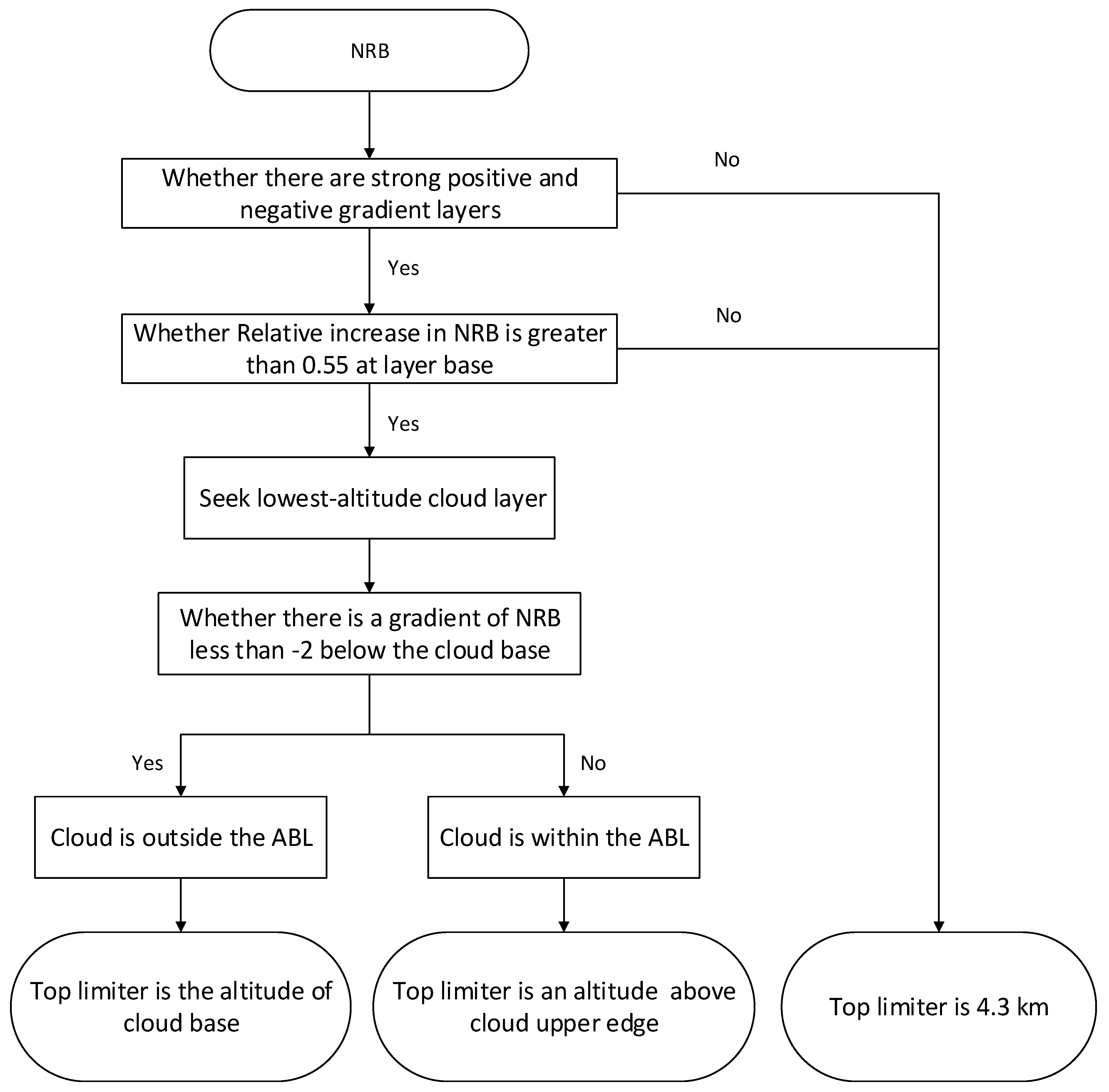
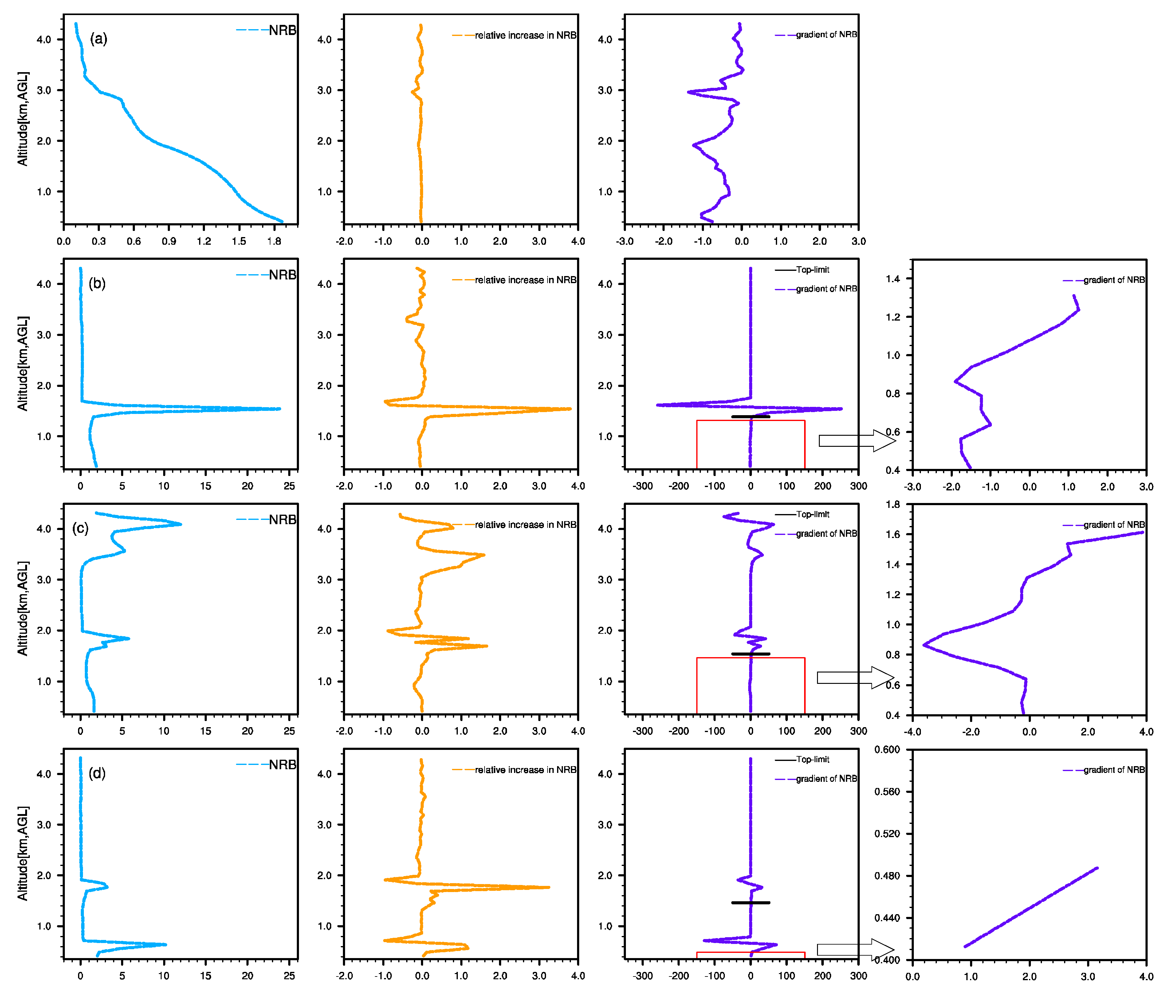
3.2. The Detailed Process for Improving the ABLH Determination

To eliminate the influence of cloud and RL, there are three major steps:

Firstly, it is important to accurately identify the cloud layers and RL on the signal profile. Backscatter signals tend to decrease linearly with height within the ABL, but increase upon interacting with clouds, elevated aerosol layer (such as RL), or random noise. Generally, the cloud base was defined as the height at which the backscatter signal reaches the maximum value [54]. Meanwhile, the strongest negative gradient often appears near the upper edge of clouds [55]. As an elevated high concentration aerosol layer, RL often occurs above the surface aerosol layer in the morning and the aerosol concentration strongly decreases near its top. That is, when the cloud layer or RL exists, a strong positive gradient with a strong negative gradient located above it can be simultaneously observed. Based on this characteristic, the cloud layers or RL can be found by seeking pairs of strong positive and negative gradients in the NRB profiles. In addition, Campbell [22] noted that for a cloud boundary to be observed, a one or two-bin relative increase in the NRB ($\left(X\left(z+\Delta z\right)-X\left(z\right)\right)/X\left(z\right)$) of at least 55% is required. Testing the empirical threshold based on many cloud cases proves that the threshold is applicable over SACOL. In this study, the strong gradient layers are identified as clouds while the relative increase in the NRB at the base of the layer is greater than or equal to 55%. Different to cloud, the magnitude of the lidar signal backscattered by RL is close to that by the near-surface aerosol layer. If the average value of the signal within the strong gradient layer is less than three to five times the average value of the signal below the bottom of the strong gradient layer, the strong gradient layer is identified as RL.

Secondly, it is necessary to classify whether the cloud caps the ABL or is decoupled from the ABL after cloud identification. To identify the lowest-altitude cloud, when the cloud layer is decoupled from the ABL, there must be a strong decrease in the signal below the cloud base reflecting the ABL structure. Instead, when the ABL is capped by the cloud, the aerosol concentration below the cloud base should be uniform vertically because of well mixing. Based on many cloudy cases, it was found that for the MPL signal profile over SACOL, if clouds are visually located above the top of the ABL, a strong signal gradient of at least less than −2 generally exists below the bottom of the cloud. Therefore, in this study, if there is at least one signal gradient that is less than the empirical threshold of −2 below the lowest cloud base, the cloud is classified as outside the ABL. In contrast, the cloud is thought to cap the ABL top.

The last step is to determine the top limiter altitude. When the lowest-altitude cloud caps the ABL, the top limiter is the altitude where a positive signal gradient first appears above the lowest cloud upper edge; it is really necessary and useful if there are more than one cloud layers. Conversely, if the lowest-altitude cloud is above the ABL, the lowest-altitude cloud base is considered to be the top altitude limiter. For a situation in which no cloud layers were identified, 4.3 km was considered to be the altitude limiter as the lidar signal only below the altitude was used in the study. A simpler flowchart for determination of the top altitude limiter aimed at cloud is presented in Figure 3. For RL in the morning, the top limiter is defined as the altitude of the strongest positive gradient below the RL top. The ABLH will be found below the top limiter altitude and it is expected to effectively eliminate the interference by cloud and RL.

Figure 4 plots the NRB, the relative increase in NRB ($\left(X\left(z+\Delta z\right)-X\left(z\right)\right)/X\left(z\right)$), and gradient of the NRB ($d\left(X\left(z\right)\right)/d\left(z\right)$) with the determined top limiter in four typical cloudy situations. Figure 4a,b are plotted at 14:15 and 10:15 LST on 09 June 2007, and Figure 4c,d are plotted at 13:45 and 10:15 LST on 28 October 2007, respectively. Figure 4a illustrates an example of a cloud-free ABL. Under this condition, the NRB decreases nearly linearly with height, as the NRB gradient and relative increase in NRB are both close to zero. In such situations, the altitude limiter is 4.3 km AGL. In Figure 4b, a sharp increase at approximately 1.4 km AGL and a sudden decrease at 1.6 km AGL are observed in the NRB, which correspond to the greatest positive gradient and strongest negative gradient appearing in the gradient profile. A relative increase in the NRB that is much larger than 0.55 is distinctly observed at the layer base, which indicates that the strong-gradient layer is a cloud layer. Figure 4c shows an example of the two strongest gradient layers along the signal gradient profile. Near the two positive gradient heights, the relative increases are both greater than 0.55, which indicates that the strongest gradient layers are both clouds. Moreover, below the cloud base in Figure 4b,c, some signal gradients (at approximately 1.0 km AGL) less than −2.0 occur (shown as the last column), which proves that the lowest-altitude clouds are above the ABL top and the heights of the cloud base are regarded as the top limiters (black solid lines). Figure 4d also shows two cloud layers, which are similar to those in Figure 4c. The difference is that the signal is continuous and there is no strong negative signal gradient less than −2.0 below the lowest altitude cloud base, which demonstrates that the lowest-altitude cloud caps the ABL. In such a situation, the top altitude limiter is defined as the height at which a positive gradient first appears above the upper edge of the cloud.

After eliminating the influence of cloud and RL, the interference by the local signal structure, such as that caused by the advection aerosol layer, must be taken into consideration, especially when gradient-based methods, such as HM, are used. Generally, the HM determines the ABLH as the altitude where the covariance transform ($w_f$) between the lidar signal and wavelet reaches a maximum. In this study, the determined height did not always corresponds to the maximum of the covariance transform. At the moments in the presence of elevated aerosols layers (not including RL) or local signal noise, the $w_f$ is ordered from largest to smallest in the vertical, the altitude is the determined ABLH at which a larger $w_f$ occurs, meanwhile, the height is closest to the ABLH at the former moment. That is, the difference between the determined ABLH at two adjacent moments (10 min intervals) is less than 0.3 km. Relative to HM, the CFM generally produces a stable ABLH and is less affected by the local signal structure. After these constraints, if the ABLH determined by HM or CFM still present significant discontinuity at a moment, it is replaced by the average of the former and later retrievals.

3.3. The Evaluation Method

The daytime ABLH is associated with features in the vertical gradients of the atmospheric thermodynamic structure. In theory, near the ABL top, there will be a sharp increase in potential temperature and, meanwhile, a sharp decrease in specific humidity [56]. The level of the strongest theta gradient is indicative of a transition from a convectively less stable region below to a more stable region above [8]. The theta-gradient is used to determine the ABLH for evaluation of the height retrieved from the above lidar-based methods, but meanwhile, the specific humidity profile is taken into consideration to ensure that there is no significant error in radiosonde-determined ABLH.

4. Results

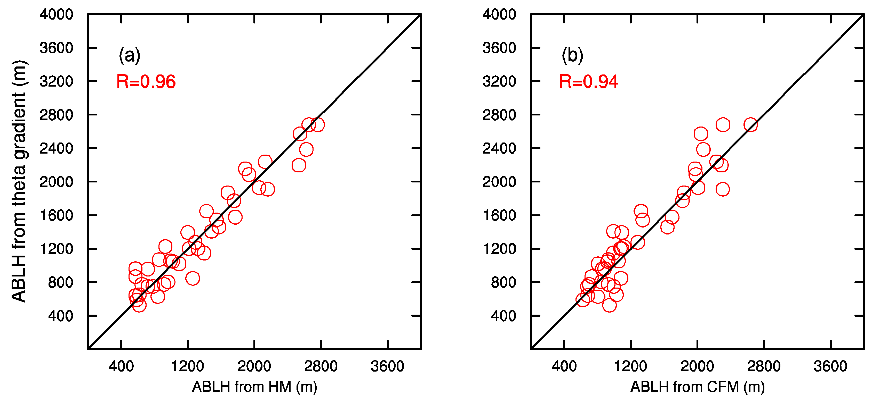
4.1. Comparisons between Lidar and Radiosonde Measurements of ABLH

The L-band radiosonde could provide accurate thermodynamic profiles, such as temperature and humidity, for the troposphere [57,58]. The ABLH determined from radiosonde-derived profiles are usually used to evaluate the ABLH retrieved from other measurements [14,59,60]. This study also evaluated the accuracy of lidar-measurements of ABLH by comparison with the radiosonde-determined ABLH. At 00:00 UTC (08:00 LST), ABLH is often a few hundred meters where the lidar signal is inaccurate because of the overlap factor. The radiosonde-derived profiles only at 12:00 UTC (20:00 LST) were selected to evaluate the lidar measurements of the ABLH.

ABLH determined by lidar-based methods (HM and CFM) were compared with that determined by the theta-gradient method as shown in Figure 5, Figure 6, Figure 7 and Figure 8. At 12:00 UTC on 17 January 2011 (cloud-free situation), the height determined from the theta-gradient is 1.07 km (Figure 5a), which is a little higher than the heights retrieved by lidar-based methods, 0.86 km by HM and 0.93 km by CFM, respectively (Figure 5b). At 12:00 UTC on 3 September 2010, there is a cloud layer above 3.0 km. Without any limitation, the HM and CFM capture the upper edge of the cloud (between 3.1 and 3.2 km) shown as Figure 6b. With the top limiter (cloud base), the heights determined from HM and CFM are between 1.5 and 1.6 km (Figure 6c), which are very close to the theta-gradient determined ABLH (Figure 6a) and the differences are less than 0.1 km. As the cloud layer is identified, and the cloud base is determined as the top limiter, the ABLH is successfully retrieved. In addition, the determined height at 12:00 UTC on 41 cloud-free cases and 20 cloudy cases from September 2010 to November 2011 were further compared. The number of cases was limited due to the lack of lidar and radiosonde data during the period, as well as the removal of some data with observed errors. Shown as Figure 7, in cloud-free situations, the ABLH determined by HM (or CFM) have high consistencies with the radisonde-determined ABLH with a correlation coefficient of 0.96 (or 0.94), with a mean bias of 0.14 km (or 0.17 km) and with mean relative absolute differences with respect to the radiosonde retrievals of 10.5% (or 12.3%) (

Table 1. Correlation coefficients (R), absolute height differences (mean and standard deviation (std) in km) between ABLH determined by theta gradient and by the Haar wavelet covariance transform method (HM) or curve fitting method (CFM) in different situations, as well as mean value of relative absolute differences relative to theta-gradient-determined ABLH (rd, in 100%).

Situations	Method	R	mean	std	rd
Cloud-free situation	HM	0.96	0.14	0.11	10.5
	CFM	0.94	0.17	0.13	12.3
Cloudy situation (without top limiter)	HM	0.09	0.83	0.90	66.1
	CFM	0.11	0.67	0.64	53.7
Cloudy situation (with top limiter)	HM	0.74	0.28	0.24	22.3
	CFM	0.79	0.22	0.18	17.2

). The comparisons in cloudy conditions are plotted in Figure 8. Without any limitation (blue open dots), on most cases, the heights determined from HM (or CFM) are much higher than those resulting from the theta gradient, with a correlation coefficient of 0.09 (or 0.11). The mean bias is 0.14 km (or 0.17 km) with a high fluctuation of the deviation (std) of 0.90 km (or 0.64 km) (Table 1). The great difference between the lidar and radiosonde measurement of ABLH is mainly caused by the cloud layers that are decoupled with the ABL. Given the top limiter (red star), the height determined by HM (or CFM) showed better concordance with those by theta gradient with a good correlation coefficient of 0.74 (or 0.79). The mean bias between HM (or CFM) and theta gradient determined ABLH is 0.28 km (or 0.22 km) with a low std of 0.24 km (or 0.18 km), while the mean relative absolute differences with respect to the radiosonde retrievals is 22.3% (or 17.2%), below 20% on average (Table 1). Overall, the results of the comparison show that relatively reliable ABLH can be determined from the lidar data in the absence of clouds. However, cloud layers, especially those decoupled from the ABL, can seriously interfere the lidar-measurements of ABLH. The top limiter improves the ABLH determination in cloudy situations.

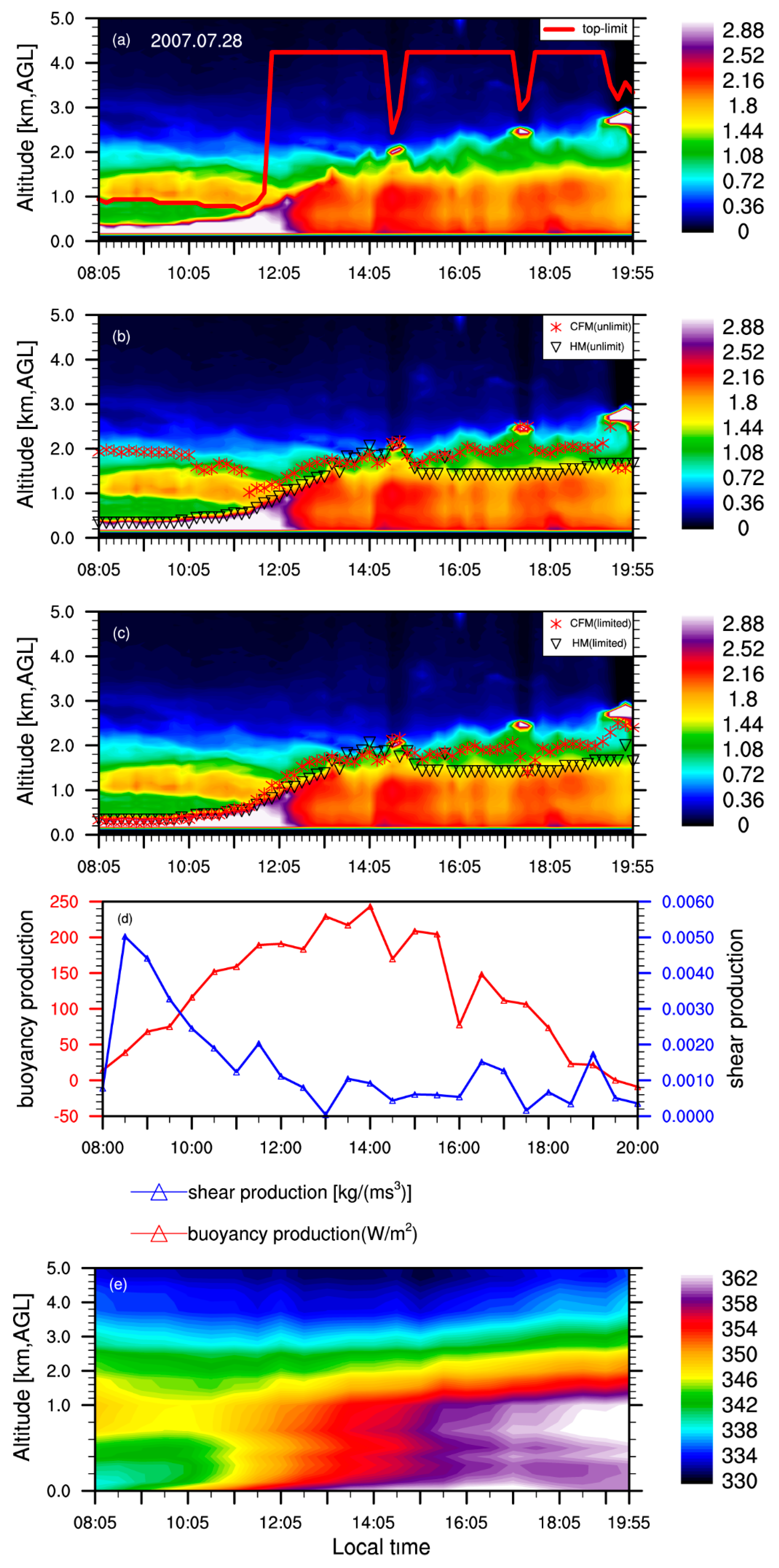
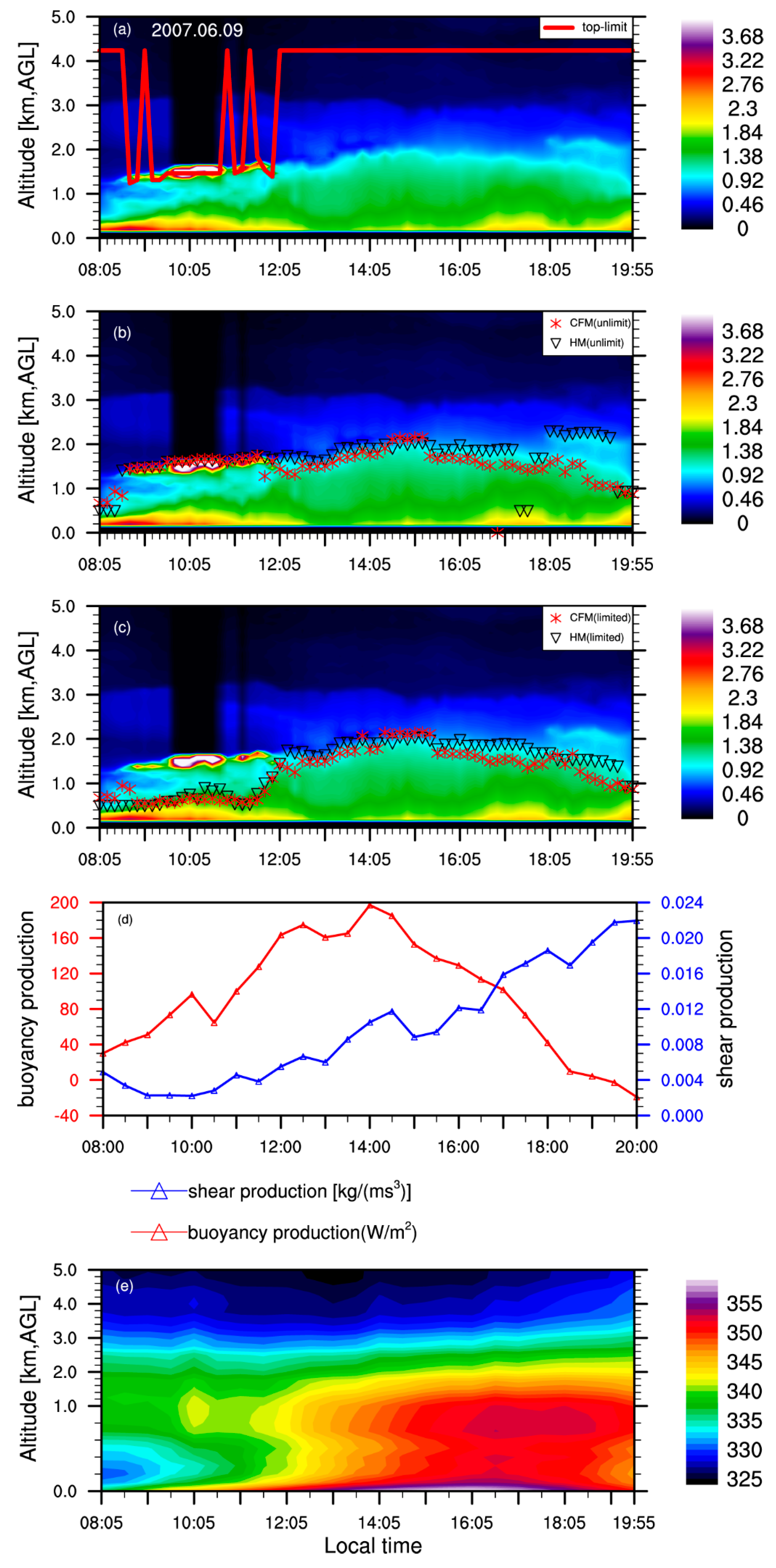
4.2. Diurnal Cycle of the ABLH

The diurnal cycle variation in ABLH were analyzed to show the proposed technique clearly, and to further test its ability for improving ABLH determination in the presence of RL, cloud layers, and local signal structures. The NRB were averaged every 10 min, correspondingly, the ABLH were calculated at a time interval of 10 min. As the nocturnal stable ABLH is usually shallower than the lidar blind zone, the study only focuses on daytime (8:05 to 19:55 LST) ABLH retrieval. To understand the diurnal cycle of the ABLH, diurnal variations in both the buoyance and shear productions of ground-layer TKE were analyzed. In addition, the distribution of ${\theta }_e$ could reflect the stratified stability, which is of importance for daily ABL developing, and the time-height distribution of ${\theta }_e$ is presented as well.

4.2.1. Residual Layer Exists in the Morning

In the morning, the RL frequently appears in the lower troposphere, with the result being that the lidar measurements of ABLH may be seriously influenced. On 28 July 2007 (Figure 9), the boundary layer diurnal variation can be divided into three stages. The time-height distribution of the NRB (Figure 9a) shows that in the morning before 11:00 LST, above the near-surface aerosol layer, there is a distinct aerosol layer between 0.8 km and 1.6 km AGL, which is a residual aerosol layer of daytime CBL the day before. During the period, the buoyancy production of surface TKE is positive and increases rapidly, the shear production decreases after 8:30 LST (Figure 9d), meaning that the mechanical turbulence weakens and the thermal forced turbulent mixing is enhanced. Simultaneously, the distribution of ${\theta }_e$ (Figure 9e) shows that the near-surface temperature is relatively low and the inversion structure is distinct, indicating a weak thermal forcing by the surface. Weak surface thermal forcing and stable stratification result in a low ABLH. For ABLH retrieval, without any limitation, while the HM performs well, the CFM captures the height close to RLH (Figure 9b). However, on other cases, when the signal negative gradient at the RL top is stronger than at the top of the near surface aerosol layer, the gradient-based methods, such as HM, are easily affected by the RL. After giving the top limiter (red solid line in Figure 9a), the low ABLH in the morning has been successfully retrieved by both CFM and HM (Figure 9c).

After 11:00 LST, the buoyancy production of surface TKE continues increasing and becomes strongest around 14:00 LST, and the shear production is weak (Figure 9d). The turbulence is mainly thermally forced. As strengthening of the near surface thermal forcing and the upward heat transport occurs, the CBL starts to grow rapidly and the strength of the capping inversion is reduced until its disappearance (Figure 9e). Correspondingly, the near-surface aerosols are transported upward and the aerosols are well mixed in the entire CBL. The ABLH retrieved from HM and CFM with the top limiter clearly shows the CBL growth process (Figure 9c). At approximately 15:30 LST, the buoyancy production of ground-layer TKE starts to decrease rapidly, but remains positive until 19:30 LST (Figure 9d). The lidar signal shows that the CBL no longer develops since 14:00 LST and the HM and CFM successfully determined the stable ABLH in the afternoon (Figure 9c).

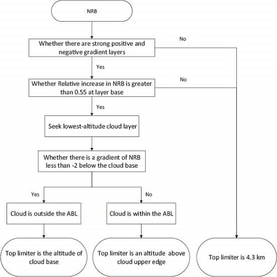
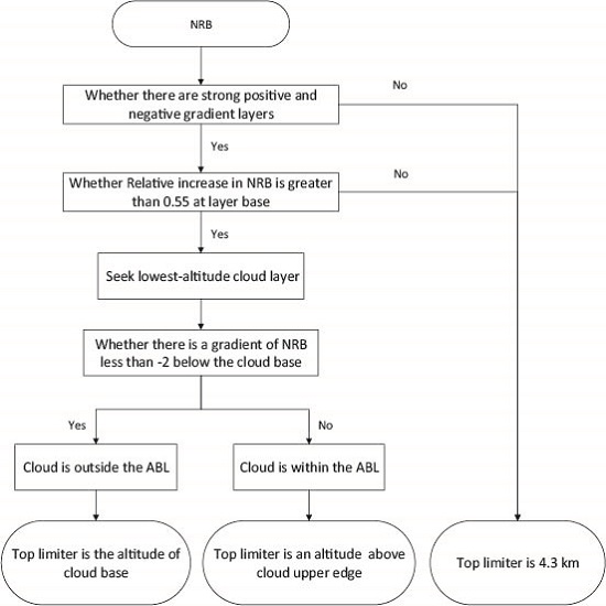
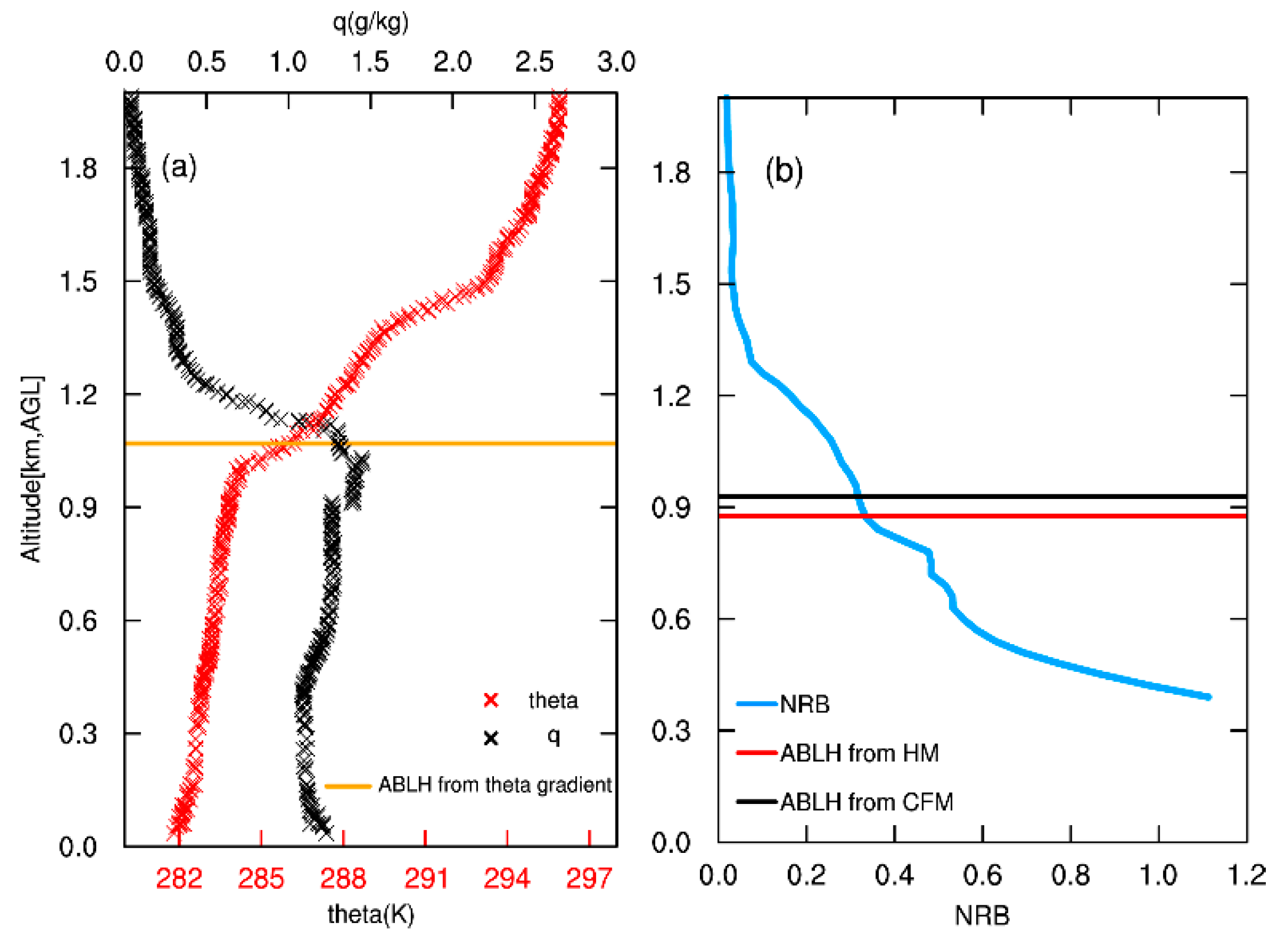
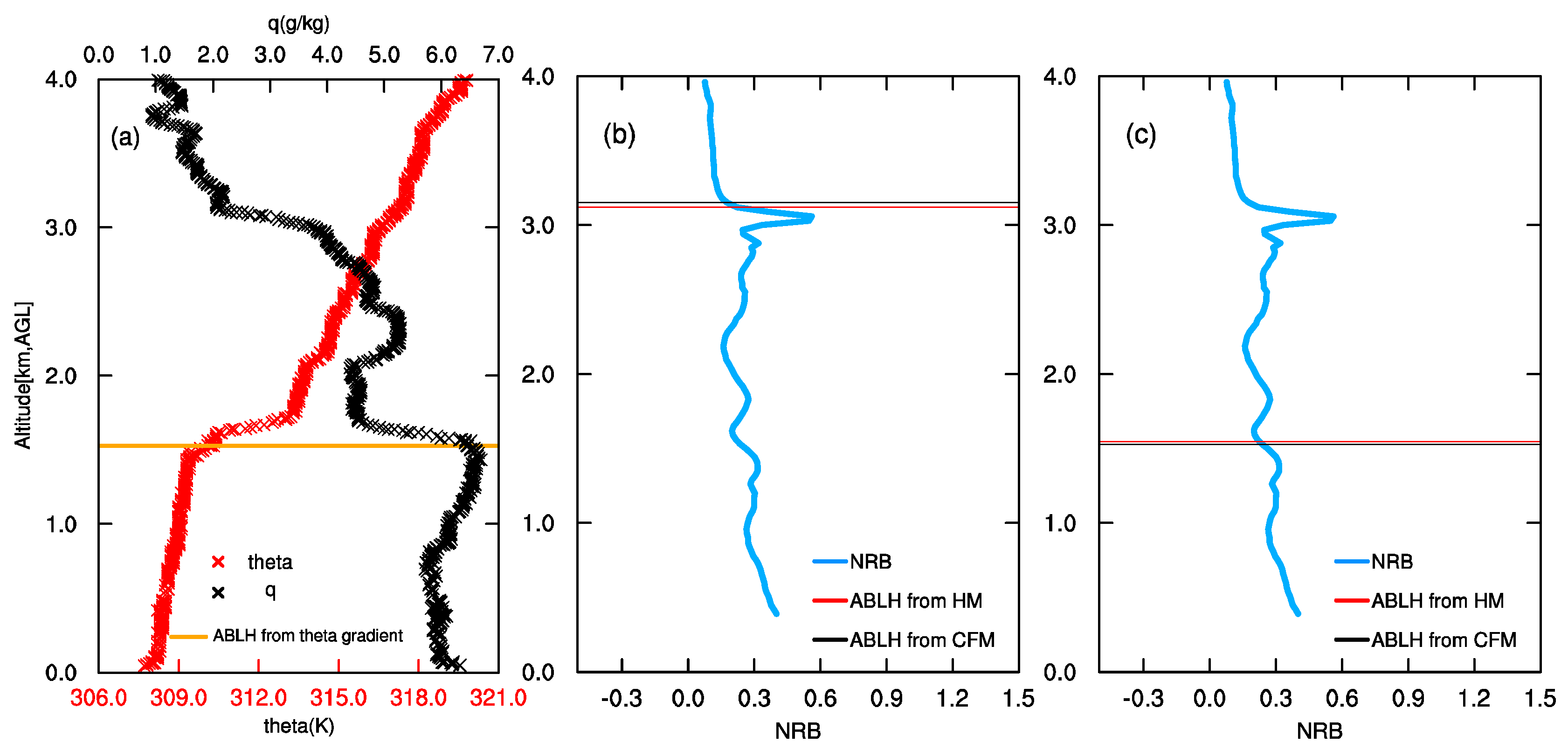
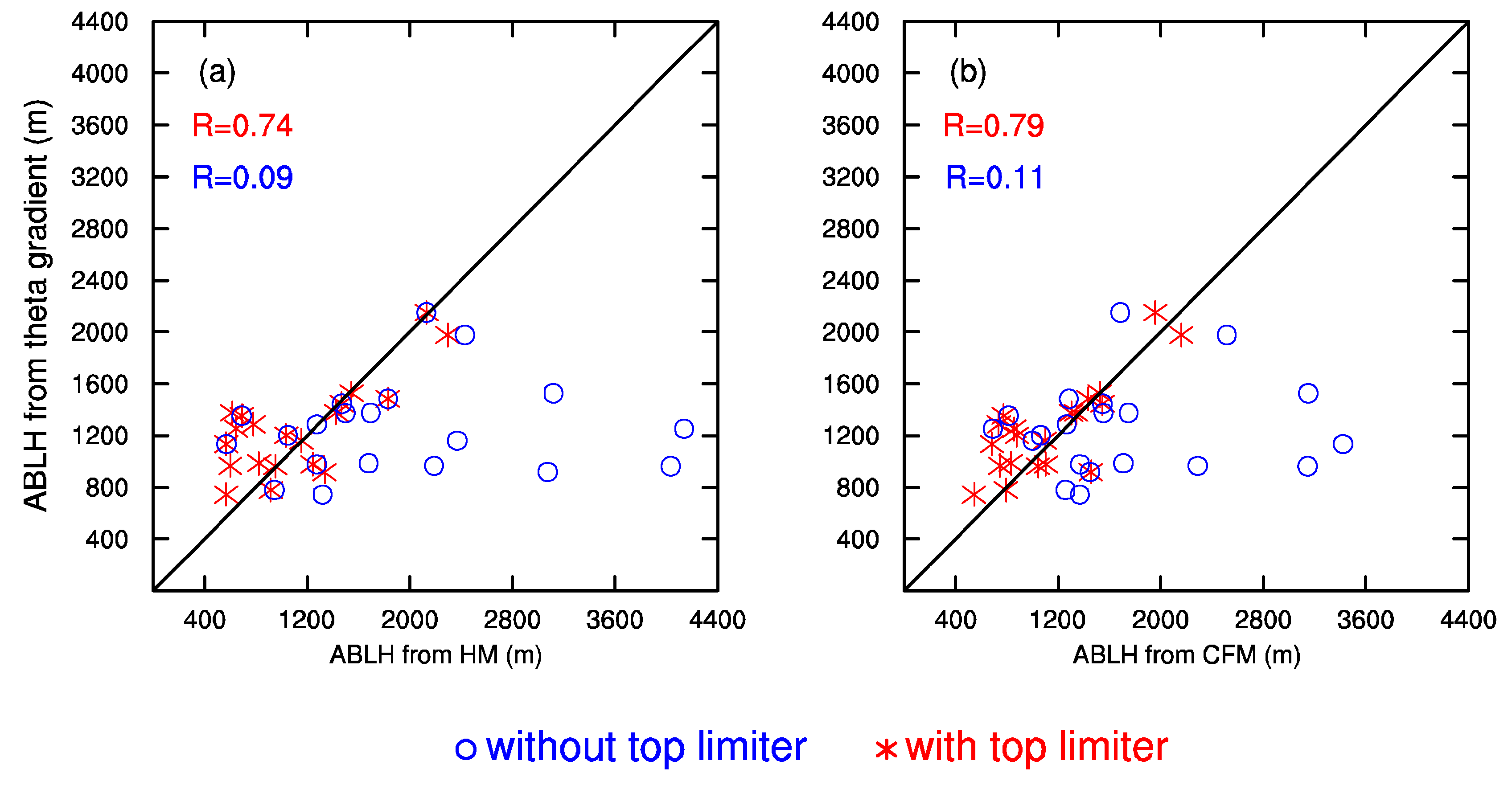
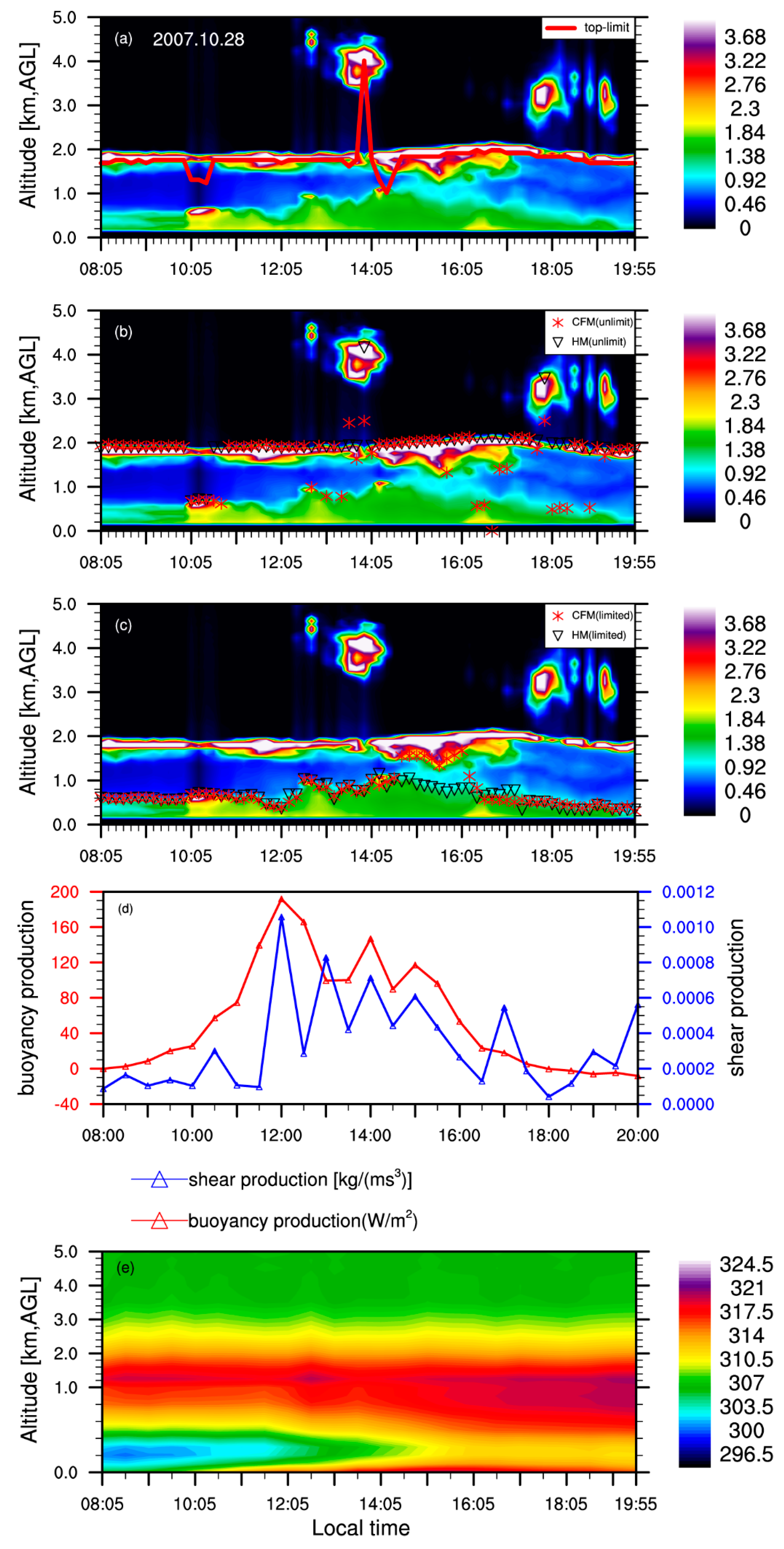
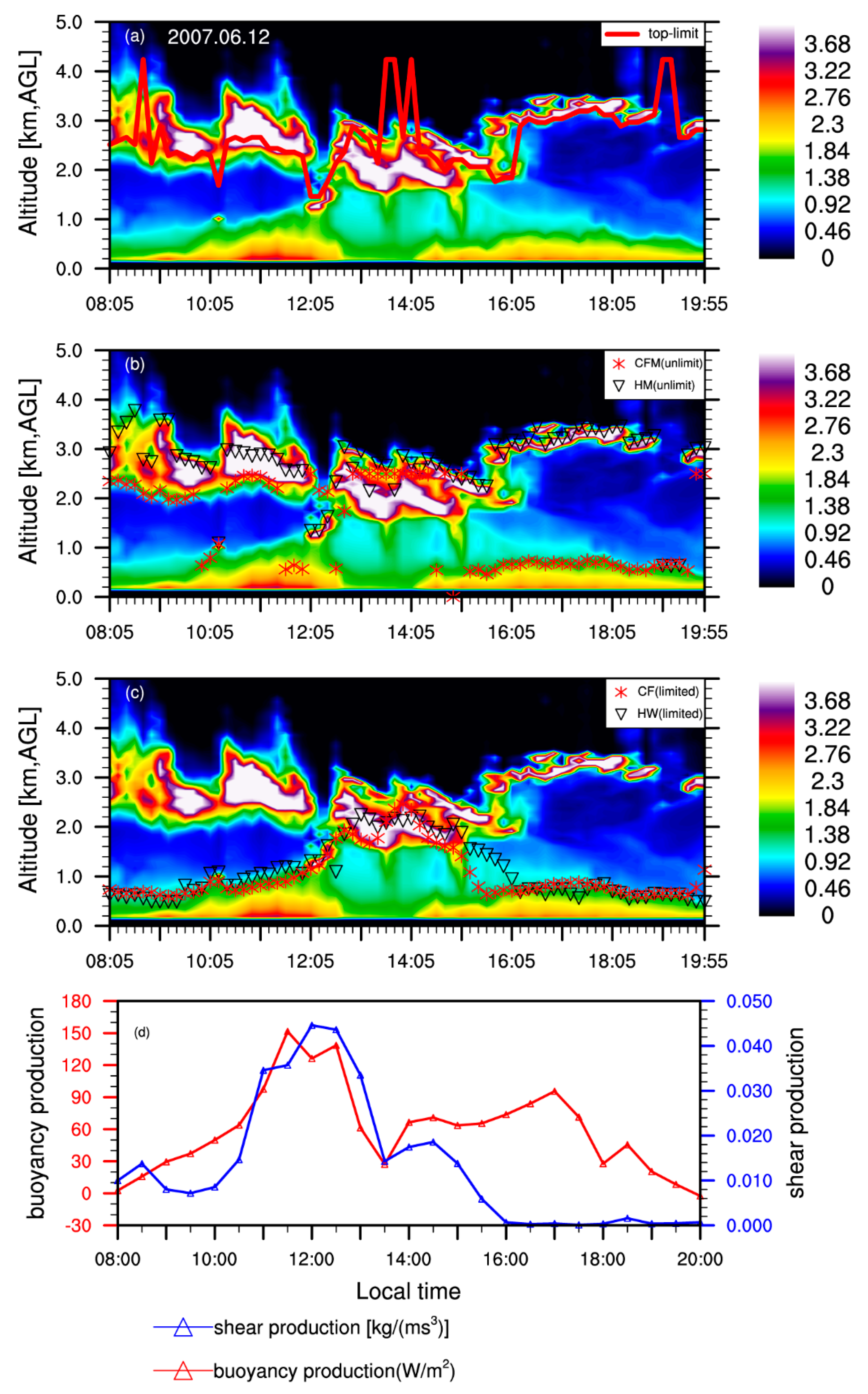
4.2.2. ABLH Retrieval in Cloudy Situations

Three cases are presented below (Figure 10, Figure 11 and Figure 12) showing the ABLH diurnal variation in different cloudy situations, and the potential of the technique proposed in this study for identifying cloud layers and eliminating their effect is discussed.

On 09 June 2007, there is a cloud layer above 1.2 km AGL between 9:00 and 11:00 LST (Figure 10a), which is presented as a white region, and above it the signal is completely attenuated. The cloud layer is followed by clear sky conditions throughout the day. Below the cloud base, there is a distinct surface aerosol layer and a strong signal negative gradient, indicating that the cloud is decoupled from the ABL. The cloud seriously influences the ABLH determination as HM and CFM capture the upper edge of the cloud (Figure 10b). Before 11:00 LST, both buoyancy and shear production of the ground-layer TKE strengthen over time (Figure 10d). There is a deep inversion layer and the upper levels are gradually heated (Figure 10e). After defining the cloud base as the top limiter altitude, the HM and CFM are able to accurately capture the slowly increasing ABLH as shown in Figure 10c.

Later, both buoyancy and shear productions of surface TKE continue to increase quickly (Figure 10d). At approximately 14:00 LST, the capping inversion is completely eroded (Figure 10e). Correspondingly, during this period, the lidar signal clearly shows the CBL growth process. As the CBL grows, the aerosols are transported upward and are well mixed within the CBL (Figure 10a). From14:00 to 18:00 LST, the buoyancy production decreases rapidly, but remains positive (Figure 10d), meaning that the CBL no longer develops further. The temperature tends to be well distributed in the vertical (Figure 10e). The signal shows that the ABLH remains nearly constant (Figure 10a). After 18:00 LST, the solar radiation decreases, and the surface begins to cool. The downward heat flux induces a weak capping inversion (Figure 10e) and the ABLH begins to descend as shown by lidar measures in Figure 10a. For the cloud-free situation after 11:00 LST, both HM and CFM successfully retrieve the ABLH. During 18:20 and 19:40 LST, the HM is originally affected by the local signal structure possibly caused by aerosol advection appearing at approximately 2 km AGL (Figure 10b). However, after considering temporal continuity, a more reasonable ABLH is retrieved as shown as Figure 10c.

On the second case of 28 October 2007 (Figure 11), there is a thin cloud layer above 1.7 km AGL, which exits throughout the entire day. Below the cloud base, the lidar signal distributes discontinuously in the vertical, and there are strong negative gradients (Figure 11a). The cloud is decoupled from the ABL. During most of the time, without any limitation, the HM and CFM capture the upper edge of the cloud, but falsely retrieve the true lower ABLH (Figure 11b). The time-height cross-section of the ${\theta }_e$ (Figure 11e) shows that there is strong and deep capping inversion throughout the entire day, and after 14:00 LST, the strength of the inversion layer gradually weakens, but is never completely eroded. The stable stratification limits the growth of ABL and the ABLH is low throughout the day (Figure 11c). At 10:00 LST, there is a lower cloud layer located at approximately 0.6 km AGL, the lidar backscatter is largely uniform below the cloud base, and the cloud caps the top of ABL. The determined ABLH is consistent with the upper edge of the lowest-altitude cloud. Between 15:00 and 18:00 LST, the CFM determines the ABLH at the cloud base height, which is a little higher than that determined by HM.

Figure 12 shows another case, 12 June 2007, which is a cloudy day. Without any limitation, the HM and CFM both capture the upper edge of the cloud (Figure 12b). Because of the thick cloud layers, the temperature and water vapor profiles provided by the radiometers are of poor quality, and only ground-layer TKE is considered. Before 12:00 LST, below the cloud base, the signal decreases distinctly and a strong negative gradient exists. The cloud is above the ABL top and the height of the cloud base is determined to be the top limiter (Figure 12a). Both buoyancy and shear productions of surface TKE are enhanced continuously (Figure 12d), and the ABLH increases due to both thermal and possibly also mechanical turbulence. Between 12:00 and 14:00 LST, the presence of the cloud layer results in the surface sensible heat flux decreasing rapidly (Figure 12d). On the other hand, the shear production of surface TKE decreases rapidly because of both the wind shear and momentum flux decrease (not shown). These phenomenon indicate that the boundary layer becomes homogeneous during the period likely due to the radiational cooling from the cloud promoting turbulent mixing [10,61]. Therefore, the aerosol concentration below the cloud base is well mixed and the cloud caps the ABL top (Figure 12a). The ABLH should be the same as the height of the cloud upper edge. Between 14:00 and 17:00 LST, as the cloudiness decreases, the surface sensible heat fluxes increase again, and the shear production of surface TKE continues decreasing after strong mixing (Figure 12d). Although surface thermal forcing increases, the promoting effect caused by the cooling at the cloud top weakens, which results in an overall reduction in the ABLH. After 17:00 LST, the cloud layer basically disappears, and with the shotwave radiation decreasing, the surface sensible heat flux decreases, and the ABLH decreases further. This case shows that the development mechanism of the ABL is relatively complex in cloudy situations, and the CBL could be forced by both mechanisms of surface heating and the radiational cooling from clouds. For the entire day, as presented in Figure 10c, after giving the top limiter altitude, both HM and CFM determine the ABLH with a reasonable level of accuracy.

Above all, the elevated aerosol layers, such as RL in the early morning as well as cloud layers, produce serious interference on lidar measurements of ABLH. The top limiter proposed in this study performs well on eliminating the disturbance of RL and the cloud layer. Meanwhile, the operation for controlling the interference of local signal structure in multiple aerosol layers to guarantee the temporal continuity is effective. Thus, the diurnal variation of ABLH can be successfully determined by HM and CFM, and the determined results by the two lidar-based methods show good agreement on the four selected cases with a mean correlation coefficient higher than 0.99, with a mean bias of 0.22 km and a low fluctuation of deviation (see

Table 2. Correlation coefficients (R) and absolute height differences (mean and standard deviation (std) in km) between ABLH retrieved by HM and CFM based on lidar data of four selected cases.

Date	R	mean	std
2007.07.28	0.998	0.25	0.21
2007.06.09	0.993	0.32	0.37
2007.10.28	0.993	0.13	0.22
2007.06.12	0.997	0.16	0.15

).

5. Discussion

Lidar is a powerful instrument for determination of the atmosphere boundary layer, but special designed algorithms are necessary to determine ABLH in conditions, such as appearance of cloud, elevated aerosol layers, local signal structure, or noise. The method explored in the study performs well on improving lidar measurements of ABLH in the appearance of cloud, elevated aerosol layers, local signal structure, or noise. However, the limitation of the technique is unavoidable. Firstly, in this study, cloud layers were divided into two situations according to their locations, one is outside the ABL and the other is within the ABL. When the cloud is within the ABL, it caps the ABL top in default and the upper edge of the cloud is defined as the ABLH. However, in fact, in some rare cases, some cloud layers are within the ABL, but not at the ABL top. In such a situation, it is really difficult to accurately determine ABLH based on lidar data, and of course, defining the cloud upper edge as the ABLH is not appropriate. Secondly, two thresholds were used when determining the top limiter to eliminate the cloud interference, one is for cloud layer identification, and the other is for classifying if the cloud is outside the ABL. The determination of the threshold relies on statistics and experience, and the threshold determined over SACOL does not necessarily apply to other observation sites. However, the principle for threshold determination is clear and reasonable, and it can be referenced for lidar measurements of ABLH in multiple-layer conditions.

6. Conclusions

Within this study, a new technique was described for elimination of the disturbance of cloud, the residual aerosol layer, and local signal structure or noise on lidar measurements of ABLH over SACOL in Northwest China. The major components of the technique are (1) identification of the RL and cloud layers from the lidar signal gradient and combining them with the relative increase in lidar signal, (2) classification of whether the cloud caps the ABL or is decoupled from the ABL by analysis of the signal continuity and finding a strong negative signal gradient smaller than an experienced threshold of −2.0 below the cloud base, (3) determination of a top limiter altitude below which the ABLH is retrieved, and (4) elimination of the influence of the local signal noise through consideration of temporal continuity. In detail, the top limiter altitude was determined as follows: When cloud caps the ABL top, the top limiter is the altitude at which a positive gradient first occurs above the upper edge of the cloud; when the cloud is decoupled from the ABL, the cloud base is defined as the top limiter; the altitude at which the strongest positive gradient occurs below the RL top is considered to be the top limiter to eliminate the RL effect. The ABLH was determined from HM and CFM below the top limiter altitude with consideration of the continuity characteristic in time.

For evaluation of the results, 41 temperature profiles in cloud-free situations as well as 20 temperature profiles under cloudy conditions at 12:00 UTC (20:00 LST) from September 2010 to November 2011 provided by radiosonde were utilized to retrieve the ABLH by the theta-gradient method to compare with the lidar-determined ABLH. In cloud-free situations, a good agreement was found between lidar-determined ABLH by HM (or CFM) and radiosonde-based retrievals with a correlation coefficient of 0.96 (or 0.94), a mean absolute bias of 0.14 km (0.17 km), and a mean relative absolute difference with respect to the radiosonde retrievals of 10.5% (or 12.3%). In cloudy situations, extensive differences appeared between the lidar-derived and radiosonde-based estimations of ABLH. The lidar-determined heights were usually much higher than radiosonde-based ABLH because lidar-based methods without a top limiter often capture the cloud upper edge. After setting the top limiter altitude, the ABLH retrieved from the two measurements showed better agreement with a correlation coefficient of 0.79 (or 0.74), a mean absolute bias of 0.28 km (0.22 km), and a mean relative absolute difference with respect to the radiosonde retrievals of 22.3% (or 17.2%) when CFM (or HM) was utilized. That is, the technique effectively eliminated the disturbance of cloud layers on ABLH determination.

The diurnal variations in the ABLH in a case with distinct RL in the morning and in three cases with different cloud situations were also analyzed. The diurnal cycle of ABLH were explained through variations in the buoyancy and shear production of surface TKE combined with the time-height distribution of the equivalent potential temperature (${\theta }_e$). When strong RL capped the near-surface aerosol layer in the morning, the strongest gradient sometimes occurred at the RL top, CFM and HM maybe captured the RL top, but not the top of the lower neutral ABL or the growing CBL. Taking the altitude of the strongest positive gradient below the RL top as the top altitude limiter can effectively control the RL influence on the ABLH retrieval. In cloudy situations, the HM and CFM usually obtained the upper edge of the cloud, but could not accurately capture the true ABLH because of the strong decrease in the signal caused by the cloud layers. Below the top limiter, the diurnal variations in the ABLH on four selected cases retrieved from the HM and CFM agreed well with a mean correlation higher than 0.99 and a mean bias of 0.22 km, and the results were consistent with surface TKE production combined with the time-height distribution of the ${\theta }_e$. In addition, for the diurnal cycle of ABLH, considering the temporal continuity characteristic to reduce the interference of local multiple aerosol layers or signal noise was necessary. The case analysis also shows that, when clouds caps the ABL, the convective boundary layer could be forced by both the heating of the surface and the radiational cooling from the cloud.

References

1. Stull, R.B. An Introduction to Boundary Layer Meteorology. Atmos. Sci. Libr. 1988, 8, 89. [Google Scholar]
2. Betts, A.K. Climate-Convection Feedbacks: Some Further Issues. Clim. Chang. 1998, 39, 35–38. [Google Scholar] [CrossRef]
3. Culf, A.D. Equilibrium evaporation beneath a growing convective boundary layer. Bound.-Layer Meteorol. 1994, 70, 37–49. [Google Scholar] [CrossRef]
4. Therry, G.; Lacarrère, P. Improving the Eddy Kinetic Energy model for planetary boundary layer description. Bound.-Layer Meteorol. 1983, 25, 63–88. [Google Scholar] [CrossRef]
5. Maronga, B.; Raasch, S.J. Large-Eddy Simulations of Surface Heterogeneity Effects on the;Convective Boundary Layer During the LITFASS-2003 Experiment. Bound.-Layer Meteorol. 2013, 146, 17–44. [Google Scholar] [CrossRef]
6. Hu, X.M.; Nielsengammon, J.W.; Zhang, F. Evaluation of Three Planetary Boundary Layer Schemes in the WRF Model. J. Appl. Meteorol. Climatol. 2010, 49, 1831–1844. [Google Scholar] [CrossRef] [Green Version]
7. Seibert, P.; Beyrich, F.; Gryning, S.E.; Joffre, S.; Rasmussen, A.; Tercier, P. Review and intercomparison of operational methods for the determination of the mixing height. Atmos. Environ. 2000, 34, 1001–1027. [Google Scholar] [CrossRef]
8. Seidel, D.J.; Ao, C.O.; Li, K. Estimating climatological planetary boundary layer heights from radiosonde observations: Comparison of methods and uncertainty analysis. J. Geophys. Res. Atmos. 2010, 115. [Google Scholar] [CrossRef] [Green Version]
9. Hennemuth, B.; Lammert, A. Determination of the Atmospheric Boundary Layer Height from Radiosonde and Lidar Backscatter. Bound.-Layer Meteorol. 2006, 120, 181–200. [Google Scholar] [CrossRef]
10. Scipión, D.E.; Chilson, P.B.; Fedorovich, E.; Palmer, R.D. Evaluation of an LES-Based Wind Profiler Simulator for Observations of a Daytime Atmospheric Convective Boundary Layer. J. Atmos. Ocean. Technol. 2008, 25, 1423–1436. [Google Scholar] [CrossRef] [Green Version]
11. Scipión, D.; Palmer, R.; Chilson, P.; Fedorovich, E.; Botnick, A. Retrieval of convective boundary layer wind field statistics from radar profiler measurements in conjunction with large eddy simulation. Meteorol. Z. 2009, 18, 175–187. [Google Scholar] [CrossRef]
12. Beyrich, F. Mixing height estimation from sodar data—A critical discussion ☆. Atmos. Environ. 1997, 31, 3941–3953. [Google Scholar] [CrossRef]
13. Luo, T.; Yuan, R.; Wang, Z. Lidar-based remote sensing of atmospheric boundary layer height over land and ocean. Atmos. Meas. Tech. 2014, 7, 173–182. [Google Scholar] [CrossRef] [Green Version]
14. Toledo, D.; Cordoba-Jabonero, C.; Adame, J.A.; Morena, B.D.L.; Gil-Ojeda, M. Estimation of the atmospheric boundary layer height during different atmospheric conditions: A comparison on reliability of several methods applied to lidar measurements. Int. J. Remote Sens. 2017, 38, 3203–3218. [Google Scholar] [CrossRef]
15. Cohn, S.A.; Angevine, W.M. Boundary Layer Height and Entrainment Zone Thickness Measured by Lidars and Wind-Profiling Radars. J. Appl. Meteorol. Climatol. 2000, 39, 1233–1247. [Google Scholar] [CrossRef]
16. Frioud, M.; Mitev, V.; Matthey, R.; Häberli, C.H.; Richner, H.; Werner, R.; Vogt, S. Elevated aerosol stratification above the Rhine Valley under strong anticyclonic conditions. Atmos. Environ. 2003, 37, 1785–1797. [Google Scholar] [CrossRef]
17. Sicard, M.; Pérez, C.; Rocadenbosch, F.; Baldasano, J.M.; García-Vizcaino, D. Mixed-Layer Depth Determination in the Barcelona Coastal Area From Regular Lidar Measurements: Methods, Results and Limitations. Bound.-Layer Meteorol. 2006, 119, 135–157. [Google Scholar] [CrossRef]
18. Couvreux, F.; Guichard, F.; Austin, P.H.; Chen, F. Nature of the Mesoscale Boundary Layer Height and Water Vapor Variability Observed 14 June 2002 during the IHOP_2002 Campaign. Mon. Weather Rev. 2009, 137, 414–432. [Google Scholar] [CrossRef]
19. Hennemuth, B.; Linné, H.; Bösenberg, J.; Ertel, K.; Leps, J.P. Vertical profiles of water vapour fluxes in the convective boundary layer, measured by ground-based Differential Absorption Lidar and Heterodyne Doppler Lidar. In Proceedings of the 16th Symposium on Boundary Layers and Turbulence, Portland, OR, USA, 9–13 August 2004. [Google Scholar]
20. Renaut, D.; Capitini, R. Boundary-Layer Water Vapor Probing with a Solar-Blind Raman Lidar: Validations, Meteorological Observations and Prospects. J. Atmos. Ocean. Technol. 1988, 5, 585–601. [Google Scholar] [CrossRef]
21. Spinhirne, J.D. Micro Pulse Lidar. IEEE Trans. Geosci. Remote Sens. 1993, 31, 48–55. [Google Scholar] [CrossRef]
22. Campbell, J.R.; Hlavka, D.L.; Spinhirne, J.D.; Turner, D.D.; Flynn, C.J. Operational cloud boundary detection and analysis from micropulse lidar data. In Proceedings of the Eighth ARM Science Team Meeting, Tucson, AZ, USA, 23–27 March 1998; pp. 119–122. [Google Scholar]
23. Zhou, T.; Hailing, X.; Jianrong, B.; Zhongwei, H.; Jianping, H.; Jinsen, S.; Beidou, Z.; Wu, Z. Lidar Measurements of Dust Aerosols during Three Field Campaigns in 2010, 2011 and 2012 over Northwestern China. Atmosphere 2018, 9, 173. [Google Scholar] [CrossRef]
24. Xie, H.; Zhou, T.; Fu, Q.; Huang, J.; Huang, Z.; Bi, J.; Shi, J.; Zhang, B.; Ge, J. Automated detection of cloud and aerosol features with SACOL micro-pulse lidar in northwest China. Opt. Express 2017, 25, 30732–30753. [Google Scholar] [CrossRef] [PubMed]
25. He, Q.S.; Mao, J.T.; Chen, J.Y.; Hu, Y.Y. Observational and modeling studies of urban atmospheric boundary-layer height and its evolution mechanisms. Atmos. Environ. 2006, 40, 1064–1077. [Google Scholar] [CrossRef]
26. Hayden, K.L.; Anlauf, K.G.; Hoff, R.M.; Strapp, J.W.; Bottenheim, J.W.; Wiebe, H.A.; Froude, F.; Martin, J.; Steyn, D.; McKendry, I.G. The vertical chemical and meteorological structure of the boundary layer in the Lower Fraser Valley during Pacific 93. Atmos. Environ. 1997, 31, 2089–2105. [Google Scholar] [CrossRef]
27. Wulfmeyer, V. Investigation of Turbulent Processes in the Lower Troposphere with Water Vapor DIAL and Radar-RASS. J. Atmos. Sci. 1998, 56, 1055–1076. [Google Scholar] [CrossRef]
28. Steyn, D.G.; Baldi, M.; Hoff, R.M. T’he Detection of Mixed Layer Depth and Entrainment Zone Thickness from Lidar Backscatter Profiles. J. Atmos. Ocean. Technol. 1999, 16, 953–959. [Google Scholar] [CrossRef]
29. Münkel, C.; Eresmaa, N.; Räsänen, J.; Karppinen, A. Retrieval of mixing height and dust concentration with lidar ceilometer. Bound.-Layer Meteorol. 2007, 124, 117–128. [Google Scholar] [CrossRef]
30. Dang, R.J.; Li, H.; Liu, Z.; Yang, Y. Statistical analysis of relationship between daytime lidar-derived planetary boundary layer height and relevant atmospheric variables in the semiarid region in northwest China. Adv. Meteorol. 2016, 2016, 1–13. [Google Scholar] [CrossRef]
31. Brooks, I.M. Finding Boundary Layer Top: Application of Wavelet Covariance Transform to Lidar Backscatter Profiles. J. Atmos. Ocean. Technol. 2003, 20, 1092–1105. [Google Scholar] [CrossRef]
32. Davis, K.J.; Gamage, N.; Hagelberg, C.R.; Kiemle, C.; Lenschow, D.H.; Sullivan, P.P. An Objective Method for Deriving Atmospheric Structure from Airborne Lidar Observations. J. Atmos. Ocean. Technol. 2000, 17, 1455–1468. [Google Scholar] [CrossRef]
33. Sawyer, V.; Li, Z. Detection, variations and intercomparison of the planetary boundary layer depth from radiosonde, lidar and infrared spectrometer. Atmos. Environ. 2013, 79, 518–528. [Google Scholar] [CrossRef]
34. Wang, Z.; Cao, X.; Zhang, L.; Notholt, J.; Zhou, B.; Liu, R.; Zhang, B. Lidar measurement of planetary boundary layer height and comparison with microwave profiling radiometer observation. Atmos. Meas. Tech. Discuss. 2012, 5, 1965–1972. [Google Scholar] [CrossRef] [Green Version]
35. Angevine, W.M.; White, A.B.; Avery, S.K. Boundary-layer depth and entrainment zone characterization with a boundary-layer profiler. Bound.-Layer Meteorol. 1994, 68, 375–385. [Google Scholar] [CrossRef]
36. Liu, B.M.; Ma, Y.Y.; Wei, G.; Zhang, M.; Yang, J. Improved Two-wavelength Lidar algorithm for Retrieving Atmospheric Boundary Layer Height. J. Quant. Spectrosc. Radiat. Transf. 2018, 224, 55–61. [Google Scholar] [CrossRef]
37. Haeffelin, M.; Angelini, F.; Morille, Y.; Martucci, G.; Frey, S.; Gobbi, G.P.; Lolli, S.; O’Dowd, C.D.; Sauvage, L.; Xueref-Rémy, I.; et al. Evaluation of Mixing-Height Retrievals from Automatic Profiling Lidars and Ceilometers in View of Future Integrated Networks in Europe. Bound.-Layer Meteorol. 2012, 143, 49–75. [Google Scholar] [CrossRef]
38. Pal, S.; Haeffelin, M.; Batchvarova, E. Exploring a geophysical process-based attribution technique for the determination of the atmospheric boundary layer depth using aerosol lidar and near-surface meteorological measurements. J. Geophys. Res.-Atmos. 2013, 118, 9277–9295. [Google Scholar] [CrossRef] [Green Version]
39. Pal, S. Monitoring Depth of Shallow Atmospheric Boundary Layer to Complement LiDAR Measurements Affected by Partial Overlap. Remote Sens. 2014, 6, 8468–8493. [Google Scholar] [CrossRef] [Green Version]
40. Wang, C.; Shi, H.; Jin, L.; Chen, H.; Wen, H. Measuring boundary-layer height under clear and cloudy conditions using three instruments. Particuology 2016, 28, 15–21. [Google Scholar]
41. Ma, M.J.; Pu, Z.X.; Wang, S.G.; Zhang, Q. Characteristics and Numerical Simulations of Extremely Large Atmospheric Boundary-layer Heights over an Arid Region in North-west China. Bound.-Layer Meteorol. 2011, 140, 163–176. [Google Scholar] [CrossRef]
42. Canny, J. A Computational Approach to Edge Detection. IEEE Trans. Pattern Anal. Mach. Intell. 1986, 6, 679–698. [Google Scholar] [CrossRef]
43. Schween, J.H.; Hirsikko, A.; Löhnert, U.; Crewell, S. Mixing-layer height retrieval with ceilometer and Doppler lidar: From case studies to long-term assessment. Atmos. Meas. Tech. 2014, 7, 4275. [Google Scholar] [CrossRef] [Green Version]
44. Morille, Y.; Haeffelin, M.; Drobinski, P.; Pelon, J.J. STRAT: An Automated Algorithm to Retrieve the Vertical Structure of the Atmosphere from Single-Channel Lidar Data. J. Atmos. Ocean. Technol. 2007, 24, 761–775. [Google Scholar] [CrossRef] [Green Version]
45. Cimini, D.; Angelis, F.D.; Dupont, J.C.; Pal, S.; Haeffelin, M. Mixing layer height retrievals by multichannel microwave radiometer observations. Atmos. Meas. Tech. Discuss. 2013, 6, 2941–2951. [Google Scholar] [CrossRef]
46. Li, H.; Yang, Y.; Hu, X.-M.; Huang, Z.W.; Wang, G.Y.; Zhang, B.D. Application of Convective Condensation Level Limiter in Convective Boundary Layer Height Retrieval Based on Lidar Data. Atmosphere 2017, 8, 79. [Google Scholar] [CrossRef]
47. Reuder, J.; Båserud, L.; Jonassen, M.O.; Kral, S.T.; Müller, M. Exploring the potential of the RPA system SUMO for multipurpose boundary-layer missions during the BLLAST campaign. Atmos. Meas. Techn. 2016, 9, 2675–2688. [Google Scholar]
48. SACOL Science Team; Dang, R.J.; Yang, Y. Micro-Pulse Lidar Data and Elevation Data. Available online: https://data.mendeley.com/submissions/ees/edit/tgc39sk74k?submission_id=ATMENV_25544token=c0659ba0-df72-43fa-8b67-8d0c69ebb5f5 (accessed on 28 December 2018).
49. Li, H.; Yang, Y.; Hu, X.M.; Huang, Z.; Wang, G.; Zhang, B.; Zhang, T. Evaluation of retrieval methods of daytime convective boundary layer height based on Lidar data. J. Geophys. Res. Atmos. 2017, 122, 4578–4593. [Google Scholar] [CrossRef]
50. Osborne, S.R.; Johnson, D.W.; Wood, R.; Bandy, B.J.; Andreae, M.O.; O’Dowd, C.D.; Glantz, P.; Kevin, J.N.; Christoph, G.; Rudolph, J.; et al. Evolution of the aerosol, cloud and boundary-layer dynamic and thermodynamic characteristics during the 2nd Lagrangian experiment of ACE-2. Tellus Ser. B-Chem. Phys. Meteorol. 2000, 52, 375–400. [Google Scholar] [CrossRef]
51. Nicholls, S. The dynamics of stratocumulus: Aircraft observations and comparisons with a mixed layer model. Q. J. R. Meteorol. Soc. 2010, 110, 783–820. [Google Scholar] [CrossRef] [Green Version]
52. Stanković, R.S.; Falkowski, B.J. The Haar wavelet transform: Its status and achievements. Comput. Electr. Eng. 2003, 29, 25–44. [Google Scholar] [CrossRef] [Green Version]
53. Gamage, N.; Hagelberg, C. Detection and Analysis of Microfronts and Associated Coherent Events Using Localized Transforms. J. Atmos. Sci. 1993, 50, 750–756. [Google Scholar] [CrossRef]
54. Eberhard, W.L. Cloud Signals from Lidar and Rotating Beam Ceilometer Compared with Pilot Ceiling. J. Atmos. Ocean. Technol. 1986, 3, 499–512. [Google Scholar] [CrossRef] [Green Version]
55. Wang, Z.; Sassen, K. Cloud Type and Macrophysical Property Retrieval Using Multiple Remote Sensors. J. Appl. Meteorol. 2001, 40, 1665–1683. [Google Scholar] [CrossRef]
56. Garratt, J.R. Review: The Atmospheric Boundary Layer; Cambridge University Press: Cambridge, UK, 1992; pp. 89–134. [Google Scholar]
57. Tao, S. Error Analyses for Temperature of L Band Radiosonde. Meteorological 2006, 32, 46–51. [Google Scholar]
58. Bian, J.; Vömel, H.; Duan, Y.; Xuan, Y.; Lü, D. Intercomparison of humidity and temperature sensors: GTS1, Vaisala RS80, and CFH. Adv. Atmos. Sci. 2011, 28, 139–146. [Google Scholar] [CrossRef]
59. Piironen, A.K.; Eloranta, E.W. Convective boundary layer mean depths and cloud geometrical properties obtained from volume imaging lidar data. J. Geophys. Res. Atmos. 1995, 100, 25569–25576. [Google Scholar] [CrossRef] [Green Version]
60. Granados-Muñoz, M.J.; Navas-Guzmán, F.; Bravo-Aranda, J.A.; Guerrero-Rascado, J.L.; Lyamani, H.; Fernández-Gálvez, J.; Alados-Arboledas, L. Automatic determination of the planetary boundary layer height using lidar: One-year analysis over southeastern Spain. J. Geophys. Res. Atmos. 2012, 117. [Google Scholar] [CrossRef] [Green Version]
61. Rogers, D.P.; Korain, D. Radiative Transfer and Turbulence in the Cloud-topped Marine Atmospheric Boundary Layer. J. Atmos. Sci. 1992, 49, 1473–1486. [Google Scholar] [CrossRef]
Figure 1. (a) A normalized relative backscatter (NRB) profile (left) and the shape of the Haar wavelet, (b) the resulted covariance transform, w f as Δ h = 600 .
Remotesensing 11 00263 g001
Figure 2. (a) An idealized backscatter profile, and (b) a real case for the curve fitting procedure.
Remotesensing 11 00263 g002
Figure 3. Major steps for determining the top limiter to eliminate the cloud effect on atmosphere boundary layer height (ABLH) retrieval in the new technique.
Remotesensing 11 00263 g003
Figure 4. Vertical distributions of normalized relative lidar backscatter signal (NRB) (the first column), relative increase in NRB (the second column), gradient of NRB with the determined top limiter (the third column), and the gradient of NRB only below the lowest cloud layer (the last column) on typical situations: (a) Cloud-free, observed at 14:15 local standard time (LST), 09 June 2007; (b) one cloud layer is observed at 10:15 LST, 09 June 2007; (c,d) more than one cloud layers are observed, the lowest-altitude cloud in (c) (at 13:45 LST, 28 October 2007) is decoupled from the ABL while in (d) (at 10:15 LST, 28 October 2007) is within the ABL.
Remotesensing 11 00263 g004
Figure 5. Vertical profiles of (a) potential temperature (theta) and specific humidity (q) at Yuzhong site, (b) lidar NRB at SACOL (Semi-Arid Climate observatory and Laboratory). The ABLH determined using different methods are marked in each panel. The profile was observed at 12:00 UTC on 17 January 2011 (In cloud-free condition).
Remotesensing 11 00263 g005
Figure 6. Similar to Figure 5, but for a cloudy case (12:00 UTC on 3 September 2010). Vertical profiles of (a) potential temperature (theta) and specific humidity (q) at Yuzhong site, (b) or (c) lidar NRB at SACOL, the ABLH retrieved by the Haar wavelet method (HM) and curve fitting method (CFM) (b) directly, (c) below the determined top limiter.
Remotesensing 11 00263 g006
Figure 7. Comparison between radiosonde-determined (vertical coordinate) and lidar measurement (horizontal coordinate) of ABLH by HM (a) or CFM (b) on 41 cases in cloud-free situations. The correlation coefficients are represented by R. The black solid line is the 1:1 line.
Remotesensing 11 00263 g007
Figure 8. Similar to Figure 7, but in cloudy situations. The blue open dots represent the comparison results of ABLH determined by theta gradient (vertical coordinate) and determined by HM (a) or CFM (b) (horizon coordinate) without height limitation, the red stars indicate the comparison results after the top limiter is given for HM and CFM. R represents the correlation coefficients, blue represents no top limiter, and red represents with the top limiter.
Remotesensing 11 00263 g008
Figure 9. Lidar measurements of ABLH over SACOL on 28 July 2007. (a) Time-height cross-section of the NRB, red solid line is the determined top altitude limiter, (b) ABLH determined directly from the HM and CFM, (c) ABLH determined from the HM and CFM below the top limiter. (d) Diurnal cycles of buoyancy production and shear production for ground-layer turbulent kinetic energy (TKE), (e) time-height cross-section of equivalent potential temperature ( θ e ).
Remotesensing 11 00263 g009
Figure 10. Same as in Figure 9, but on 9 June 2007.
Remotesensing 11 00263 g010
Figure 11. Same as in Figure 9, but on 28 October 2007.
Remotesensing 11 00263 g011
Figure 12. Same as in Figure 9, but on 12 June 2007. The radiometrics profiling radiometer data quality were seriously affected by clouds and there was no equivalent potential temperature data available.
Remotesensing 11 00263 g012