Article

Measurement of Planetary Boundary Layer Winds with Scanning Doppler Lidar

1
School of Earth and Environmental Sciences, Seoul National University, Seoul 08826, Korea
2
Research Center for Atmospheric Environment, Hankuk University of Foreign Studies, Yongin 17035, Korea
3
School of Urban and Environmental Engineering, Ulsan National Institute of Science and Technology, Ulsan 44919, Korea
*
Author to whom correspondence should be addressed.
Remote Sens. 2018, 10(8), 1261; https://doi.org/10.3390/rs10081261
Submission received: 19 June 2018 / Revised: 7 August 2018 / Accepted: 8 August 2018 / Published: 10 August 2018
(This article belongs to the Special Issue Remote Sensing of the Atmospheric Boundary Layer)

Abstract

:
The accurate measurement of wind profiles in the planetary boundary layer (PBL) is important not only for numerical weather prediction, but also for air quality modeling. Two wind retrieval methods using scanning Doppler light detection and ranging (lidar) measurements were compared and validated with simultaneous radiosonde soundings. A comparison with 17 radiosonde sounding profiles showed that the sine-fitting method was able to retrieve a larger number of data points, but the singular value decomposition method showed significantly smaller bias (0.57 m s−1) and root-mean-square error (1.75 m s−1) with radiosonde soundings. Increasing the averaging time interval of radial velocity for obtaining velocity azimuth display scans to 15 min resulted in better agreement with radiosonde soundings due to the signal averaging effect on noise. Simultaneous measurements from collocated wind Doppler lidar and aerosol Mie-scattering lidar revealed the temporal evolution of PBL winds and the vertical distribution of aerosols within the PBL.

Graphical Abstract

1. Introduction

Understanding planetary boundary layer (PBL) winds is important for air quality modeling, because winds within the PBL have a significant influence on the dispersion and transport of aerosols and their precursors [1,2]. Winds within the PBL also play an important role in numerical weather prediction (NWP) as a major driver of PBL dynamics and mass advection [3,4]. The need to obtain realistic diurnal cycles of PBL winds has also been recognized for various environment-related problems, such as wind energy and visibility, as well as construction engineering [5]. Despite its importance, the complex structure and evolution of PBL and winds within the PBL in urban environments have been poorly understood due to lack of comprehensive observations [6].
Various remote sensing techniques have been used to continuously measure atmospheric variables, such as temperature, turbulence, winds, and aerosol distribution within the PBL [7,8]. Light detection and ranging (lidar) systems, in particular, have been used for atmospheric research since the 1960s [9,10]. With the growth of the wind energy industry, wind measuring techniques using wind Doppler lidar (WDL) systems have developed steadily and have gained widespread acceptance since the 1990s [11]. Continuous WDL observations provide information regarding the temporal evolution of wind profiles within the PBL, which is useful as input and validation data for air quality and NWP modeling. However, wind retrievals from WDL are sensitive to the strength of the signal backscattered by atmospheric particulate tracers (i.e., aerosols). Therefore, a quality check for the removal of noise from measurements and an assessment of each system’s performance are necessary [12,13].
The objectives of this study are to ensure the performance and reliability of winds measured by the scanning Doppler lidar and to investigate the evolution of wind profiles within the PBL. We firstly evaluate wind profiles from two WDL retrieval algorithms by comparison with radiosonde soundings and discuss several critical factors in the WDL wind retrieval process. Diurnal variations of wind profiles and aerosol distributions in the PBL are also investigated using simultaneous measurements of WDL and aerosol Mie-scattering lidar.

2. Instrumentation and Measurements

2.1. Principle of the Wind Doppler Lidar

A WDL utilizes the Doppler frequency shifts of photons when they are scattered by moving aerosols [14]. By measuring the frequency shift in the lidar pulse and using the following Doppler shift equation (Equation (1); [15]), it is possible to retrieve the speed at which aerosols or molecules are moving with respect to the line of sight (LOS) of the laser beam—that is, the component of the wind speed in the direction of the laser beam (the so-called radial or LOS velocity).
Δ f = f   f 0 =   2 f 0 v r / c ,
where f 0 and f indicate the frequency of the outgoing beam and returning lidar signal, respectively, v r is the radial velocity, and c is the speed of light. The meridional ( u ), zonal ( v ), and vertical ( w ) wind components are retrieved through various methods from radial velocities ( v r ) and its behavior with the LOS direction. To retrieve the wind vector ( V ), the lidar system assumes that wind is horizontally homogeneous and requires measurements of radial velocities from at least three different directions.

2.2. Wind Data Retrieval Processes

Two major measuring techniques are capable of retrieving wind vectors from radial velocity measurements: the velocity–azimuth display (VAD) technique and the Doppler beam swinging (DBS) technique [9,15,16]. The VAD technique makes a conical scan at a fixed elevation angle and retrieves wind vectors using the radial velocity azimuth distribution. The DBS technique, on the other hand, takes observations of v r at two or three different azimuth angles of fixed elevation angle and one in the vertical to retrieve the wind vector.
This study carried out a comparison of two wind retrieval methods for radial velocities from VAD scans: the sine-fitting method and the singular value decomposition (SVD) method. The sine-fitting method uses the azimuth angular distribution of radial velocity to find a fitted sine-curve function in the form noted in [15]. This is an example of such an equation:
v r = a + b cos ( θ θ m a x ) .
The wind vector is calculated using Equation (3) with the same constants as in Equation (2):
V = ( u ,   v ,   w ) =   ( b sin θ m a x / cos φ ,   b cos θ m a x / cos φ ,   a / sin φ ) .
Constants a , b , and θ m a x in Equation (2) are the offset, amplitude, and phase shift of the sine curve that best fit the VAD scan. θ and φ represent the azimuth and elevation angle of the lidar beam, respectively.
On the other hand, the SVD method solves the following equation [13]:
V r = A   V V r =   ( v r 1 v r 2 v r n ) ,   A =   ( s i n θ 1 c o s φ c o s θ 1 c o s φ s i n φ s i n θ 2 c o s φ s i n θ n c o s φ c o s θ 2 c o s φ c o s θ n c o s φ s i n φ s i n φ ) , V =   ( u v w ) .
Here, v r n is the radial velocity observed at the nth pointing direction of the WDL, at an azimuth angle of θ n and an elevation angle of φ . Vector V r is referred to as the VAD scan and the constituents ( v r n ) are the mean of radial velocities observed at the nth pointing direction. The matrix A is composed of the azimuth and elevation angle data of the LOS. In solving the overdetermined Equation (4), a method of least squares is needed, and this study uses the SVD method due to its advantages, as referred to in [13]. The matrix A is decomposed using SVD to Equation (5), which in turn is used in Equation (6) to obtain the solution V.
A = U W B T
V = ( A T A ) 1 A T V r = A + V r = B W 1 U T V r
W is a diagonal matrix with singular values of A as its diagonal elements, and A + stands for the Moore–Penrose pseudoinverse of matrix A. Equation (6) holds, because A T A is invertible.

2.3. Measurements

Measurements of PBL winds were made with a compact and portable scanning WDL manufactured by MITSUBISHI ELECTRIC (Model: LR-S1D2GA, Japan; http://www.mitsubishielectric.co.jp/lidar/products/all-fiber/index.html) at two locations in Seoul during the period from April 2016 to October 2017: the Seoul National University Gwanak campus (hereafter, referred to as ‘Gwanak’; [17]) and Jungnang [18] (Figure 1). The instrument specifications are given in Table 1. Due to its vulnerability to precipitation, the measurements were made intermittently in non-precipitating conditions. The technical specifications of the WDL operation, consistent throughout the study period, are given in Table 2. Of the scanning methods provided by the WDL system, the plan position indicator (PPI) mode, which makes a conical scan of fixed elevation angle, was used. The elevation angle was fixed at 80° due to limits in measurements at lower angles caused by obstacles (mountains and buildings), and to maximize the observation altitude range. The azimuth scanning range was set from −90° to 90° from its heading direction and scanning speed was set at 1° s−1. The range resolution was set at 75 m and the minimum range of observation was 60 m. Since the number of gates of the instrument is 20 points, the maximum detection distance from the WDL was 1560 m during the study period. Noise due to electronics (i.e., ground noise) was removed by measuring the returning signal with the laser detector covered each time the WDL system was newly set up for observation.
For the validation of the WDL performance in wind retrievals, 17 radiosonde soundings from the same site as the WDL were used for comparison. Two types of radiosondes, the Jinyang RSG-20A GPS radiosonde (Ansung, Korea; http://www.jinyangind.com/eng/system_uass.html) at Gwanak and the Meteomodem M10 radiosonde (URY, France; http://www.meteomodem.com/m10.html) at Jungnang, were used in this study. The accuracy of wind speed is 0.2 m s−1 (Jinyang RSG-20A GPS radiosonde) and 0.15 m s−1 (Meteomodem M10 radiosonde), respectively. The wind direction accuracy of the Jinyang RSG-20A GPS radiosonde is 5° for wind speeds smaller than 5 m s−1 and 2° for winds excessing 5 m s−1, while 1° for the Meteomodem M10 radiosonde.

3. Results and Discussion

3.1. Comparison of Wind Retrieval Processes

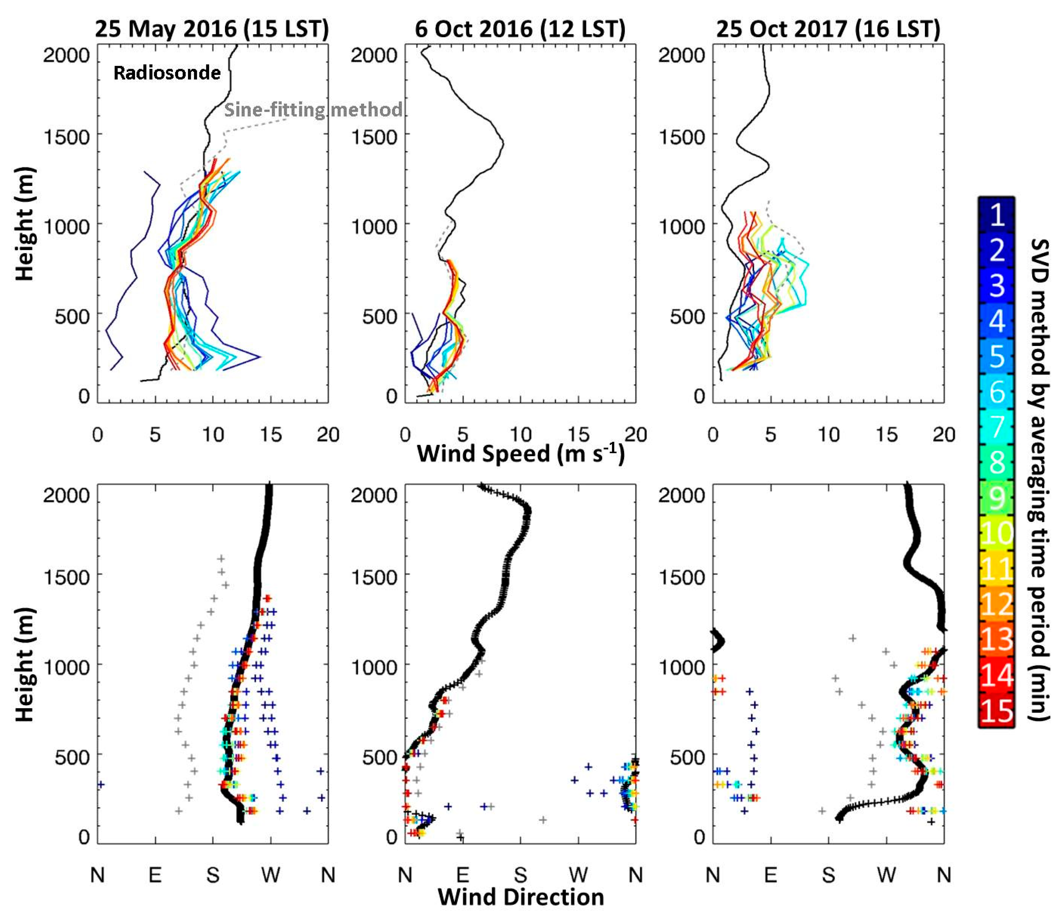
Figure 2 shows examples of comparisons of WDL wind profiles retrieved using the sine-fitting and SVD methods with those from collocated radiosonde soundings. The profiles of wind speed and wind direction by the sine-fitting method were calculated every 3 min, whereas wind profiles by the SVD method were retrieved for various time intervals to check the sensitivity of wind retrievals to the VAD scan from 1 to 15 min, as notated by different colors in Figure 2. The wind profiles seen in Figure 2 by both methods were averaged from 15 min after the start time of the radiosonde flight. The detection range of the WDL varied not only according to the atmospheric conditions, but also by the retrieval method. Because the distribution of aerosols within the PBL has a large variance according to atmospheric conditions (e.g., mixing height, stability, advection, diffusivity, etc.), the detection range of the WDL shows large variations from case to case. The sine-fitting method showed higher detection ranges than the SVD method, because the sine-fitting method was able to retrieve winds with a smaller number of radial velocity measurements than the SVD method. However, this may lead to higher uncertainty in the results from the sine-fitting method, especially in wind observations at higher altitudes, where the number of radial velocities used to retrieve per wind vector is smaller than that of lower altitudes. Differences in the detection range within the SVD method were also observed with variation in the averaging time interval. Wind profiles retrieved from longer averaging time intervals resulting in longer detection ranges can be attributed to the accumulation of data points at higher heights with increasing time. Variation in time-averaging intervals with the SVD method not only resulted in changes of the detection range, but also in the final retrieved wind speed and wind direction values. Wind profiles retrieved from different VAD scans of different averaging time intervals in Figure 2 show that retrievals with longer averaging time intervals have better agreement with radiosonde soundings.
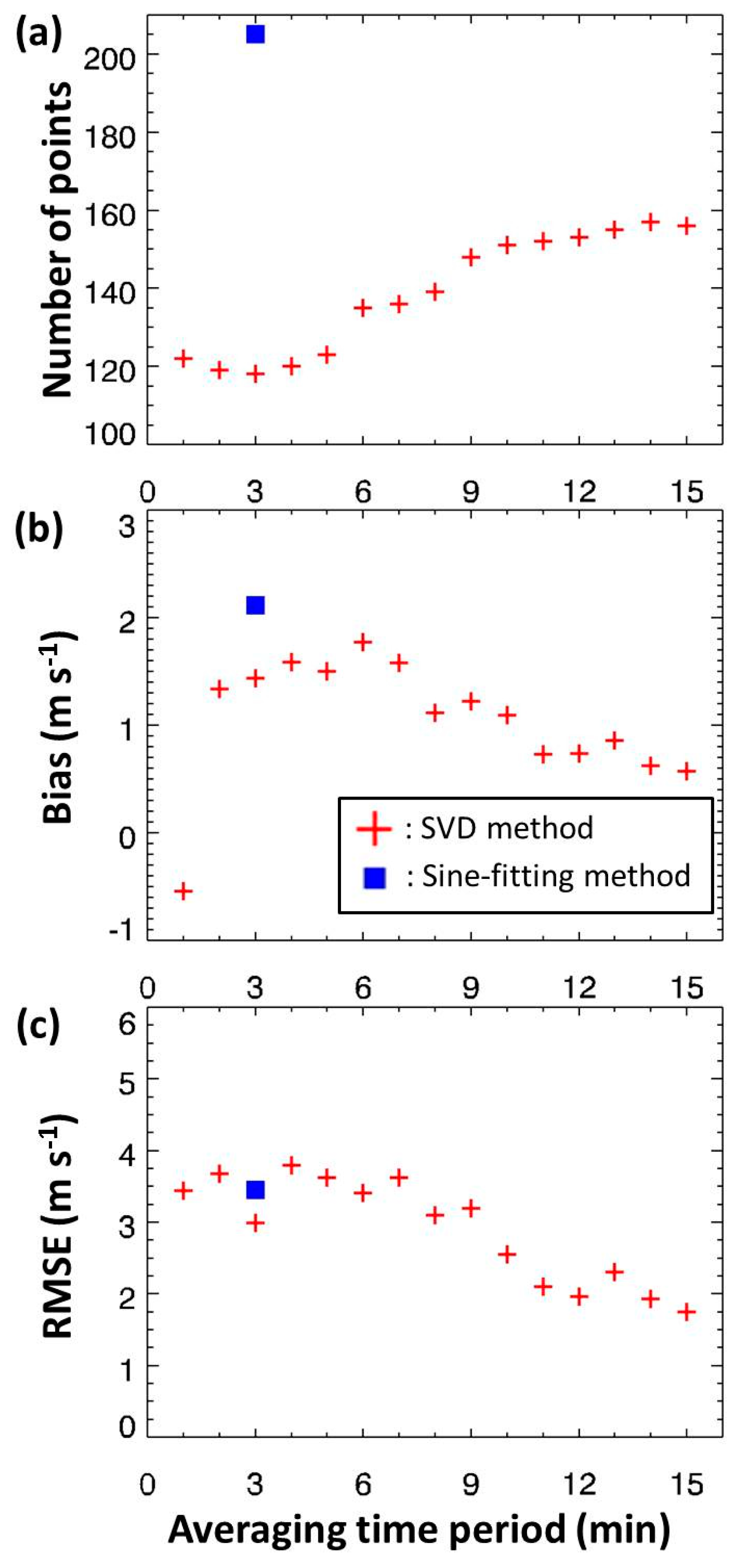
A statistical analysis was done for a comprehensive investigation of the relation between averaging time period and the wind speed/wind direction retrievals from the WDL compared with radiosonde soundings for all points from all 17 experiment data points (
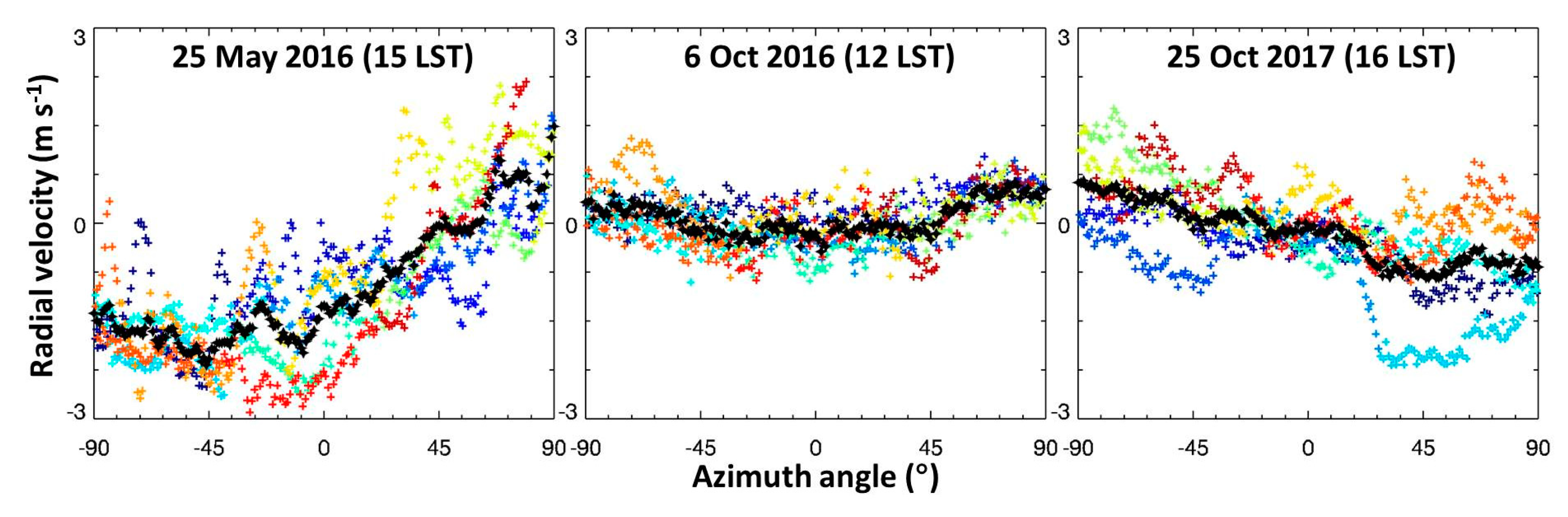
Figure 3). While the sine-fitting method allowed a larger number of simultaneous data points (205) to be collected, the maximum number of wind points retrieved using the SVD method was 157 at an averaging time interval of 14 min. This coincides with the fact that the overall retrieval range of the SVD method was shorter than that of the sine-fitting method, because the latter is insensitive to a few missing points. Notably, the SVD method fails to retrieve wind vectors for VAD scans with missing values. As the averaging time interval increases, there are fewer missing points in the averaged VAD scan, resulting in higher number of simultaneous points. The bias and root-mean-square error (RMSE) between WDL measurements and radiosonde soundings showed a decreasing tendency with longer averaging time intervals, indicating that increasing the averaging time interval had a positive effect on the accuracy of the lidar wind retrievals. This can be explained by investigating the radial velocity distribution with the azimuth angle, as shown in Figure 4. The colored points in Figure 4 indicate the radial velocity observed at the third gate (approximately 200 m altitude) at each azimuth angle of the lidar during the 15 min after the start of the flight of the radiosonde. Each color indicates the minute during which the radial velocity was measured (i.e., initial VAD scan). Because the scanning speed of the lidar was set at 1° s−1, for each azimuth, the radial velocity was measured during one second. Existing variances in the angular distribution of radial velocities during 15 min can lead to variances in the wind vectors retrieved depending on the used VAD. Radial velocities plotted in black are the average radial velocity at each azimuth angle (i.e., 15-min-averaged VAD scan). Comparing the initial VAD scan with the 15-min-averaged VAD scan shows a smoother plot for the latter. Because the WDL assumes horizontal homogeneity in winds, the smoother the VAD scan, the more stable the results. With a longer averaging time interval, the VAD scan is smoothed, and thus, the bias and RMSE compared with radiosonde soundings decrease. A significant improvement in the bias and RMSE can be noticed when the averaging time interval is longer than 11 min. Bias and RMSE with radiosonde soundings showed minimum values for wind profiles retrieved using the SVD method with 15-min-averaged VAD scans (0.62 m s−1 and 1.93 m s−1, respectively).
Considering the VAD scans in Figure 4 to be cosine functions, the amplitudes of the VAD scans are proportional to the magnitude of wind speed. Comparing the three examples given in Figure 4, the wind speed was strongest for 25 May 2016, the wind speed retrieved from the VAD scan of 25 May 2016 in Figure 4 being 5.75 m s−1. The corresponding values for the other two cases were 3.99 m s−1 and 3.62 m s−1, respectively. It should be noted that VAD scans can be affected not only by noise, but also by the horizontal homogeneity of winds. From the perspective of wind homogeneity, the 15-min-averaged VAD scan of 6 October 2016, showing the smallest variance in radial velocity with time, can be said to best represent the actual wind out of the three cases in Figure 4. In other words, small variance in radial velocity distribution with time indicates a wind field with less small-scale turbulence than VAD scans showing large variance with time.
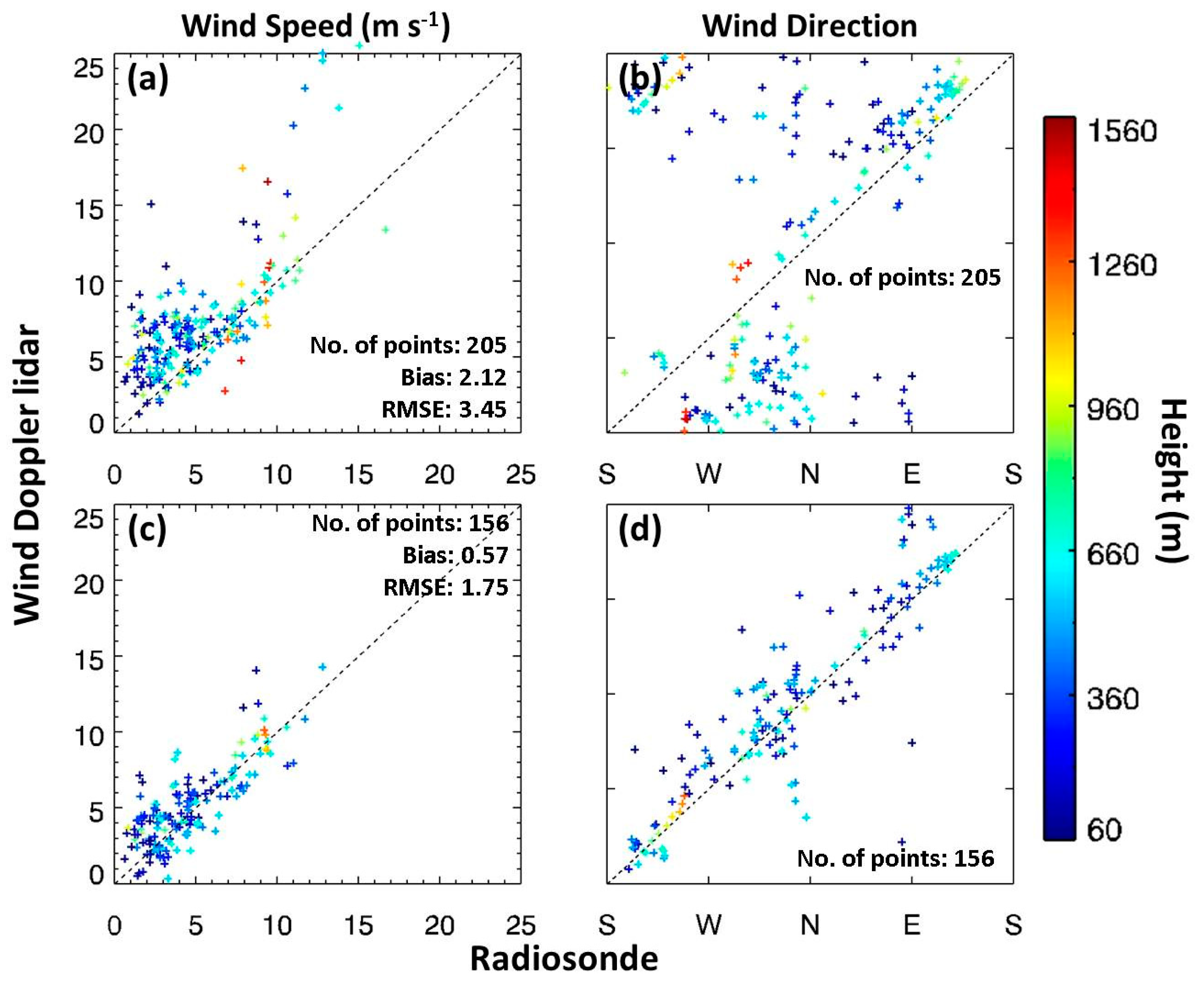
A scatterplot of radiosonde observations compared with WDL retrievals is given in Figure 5. Although the number of points is larger when using the sine-fitting method (Figure 5a,b), the bias and RMSE in wind speed show a large improvement (with the bias decreasing from 2.12 to 0.57 m s−1 and the RMSE decreasing from 3.45 to 1.75 m s−1) when using the SVD method (Figure 5c). Moreover, it should be noted that the majority of wind vectors from higher altitudes (1 km) show large bias from the radiosonde data (Figure 5a,b). This observation coincides with the discussion from Figure 2, where the sine-fitting method shows lower accuracy at higher altitudes. On the other hand, horizontal drifting of the radiosonde (0.7–4.5 km horizontal drifts during a 1.5 km ascent) may also contribute to the increase of bias between the radiosonde sounding and the WDL wind profiles with height. There is a significant improvement in wind direction results when using the SVD method (Figure 5d). Because the wind direction is calculated using the angle of the meridian ( u ) and zonal ( v ) components of wind, improvement in the wind direction can lead to the assumption that the accuracy of the retrievals of u , v , and consequently, w has undergone significant improvement.

3.2. Diurnal Variation of Winds

Diurnal variations in wind speed and direction retrieved using the SVD method on 15-min-averaged VAD scans were investigated for two cases with significantly different temporal variations in wind profiles (Figure 6 and Figure 7). 
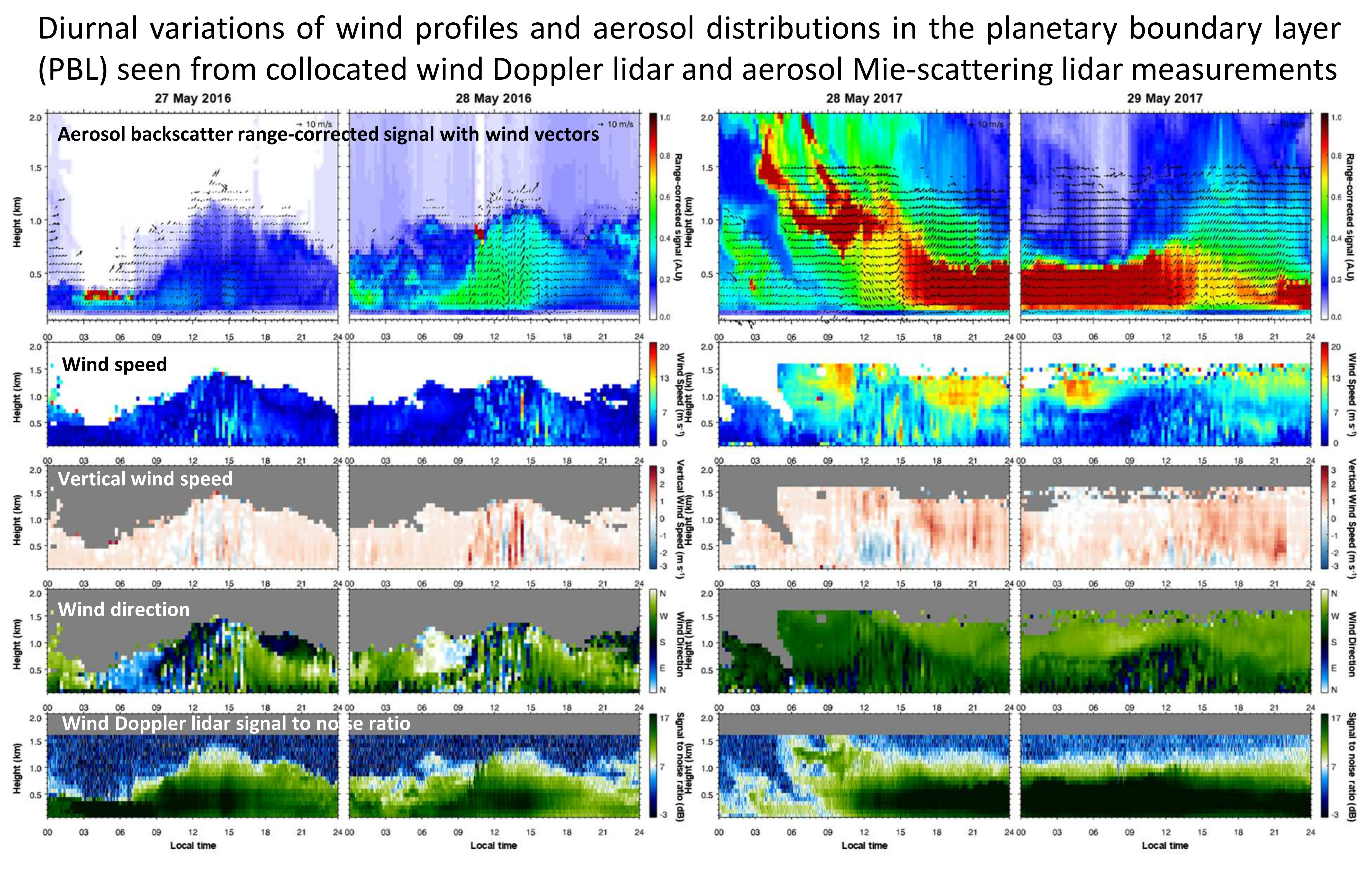
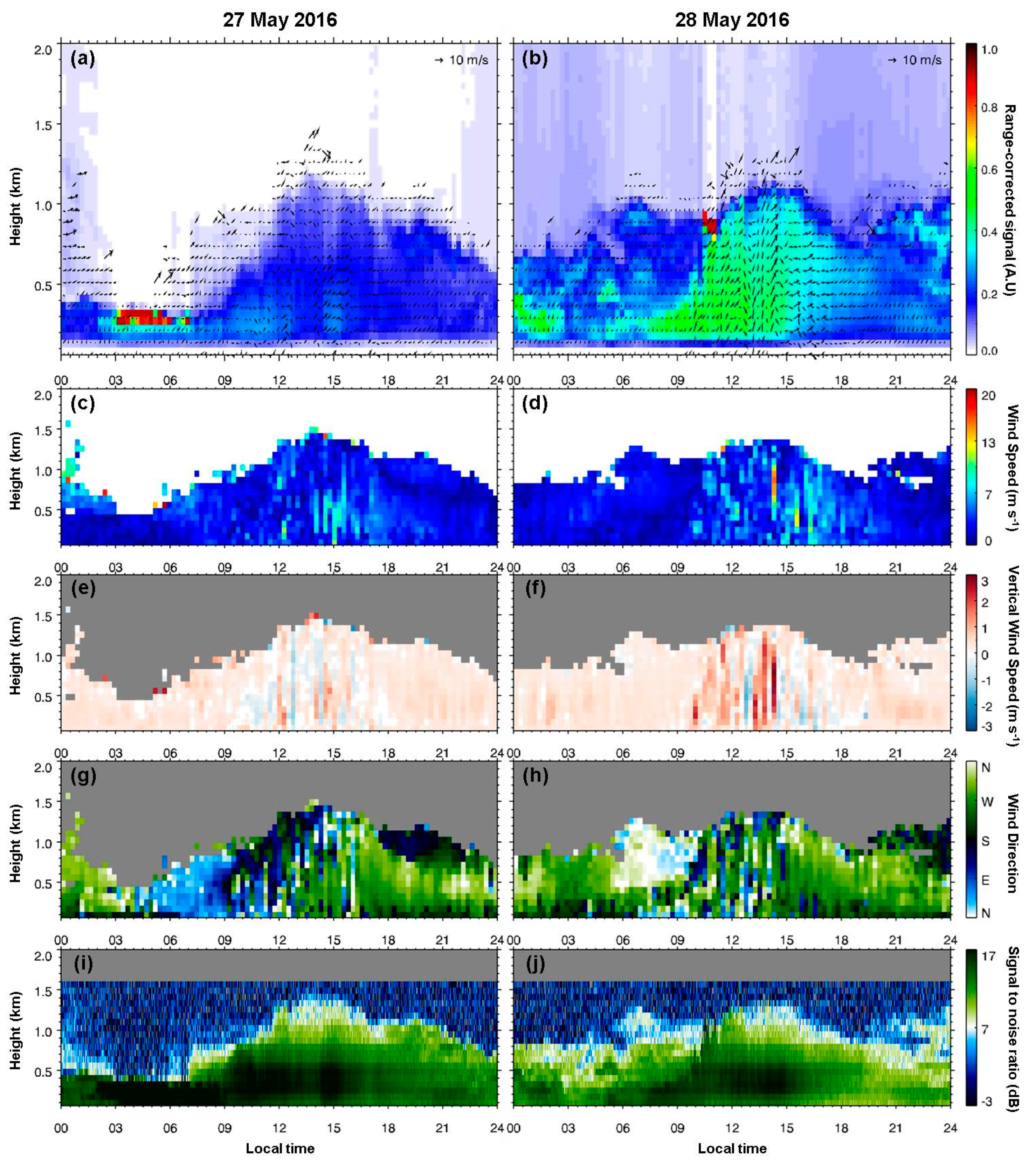
Figure 6 shows the daily plots of wind speed and direction on 27 (left panel) and 28 (right panel) May 2016, observed at the Gwanak site, during which time the wind profiles displayed characteristics close to a convective boundary layer, showing large variation in wind speed and direction between day and night as a result of the thermal heating of the surface [19]. Wind speeds were low during the night (2.28 m s−1) and higher wind speeds were observed during the daytime (10:00–17:00 local time; 3.58 m s−1). Vertical wind speed also showed similar diurnal variation. However, during the afternoon, rapid changes between updrafts and downdrafts were observed (the vertical wind speed variation of 0.32 m2 s−2 during the day was significantly larger than that during the night (0.06 m2 s−2)), implying that turbulence of the boundary layer was thermally induced. While a consistent weak updraft was observed apart from the turbulent hours, strong updrafts were observed during the afternoon of 28 May 2016. This strong updraft coincided with the sudden thickening of the aerosol layer, leading to the inference that convection played an important role in the transportation of aerosols to higher altitudes (i.e., vertical mixing of aerosols in the PBL).
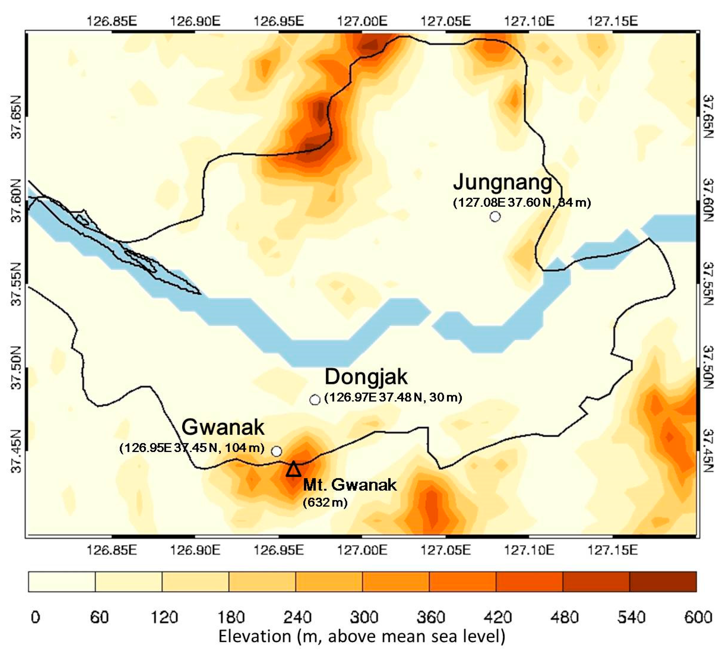
Meanwhile, the change in the diurnal wind direction during 27–28 May 2016 showed the typical pattern of valley and mountain breezes. Due to the inhomogeneity in surface heating, valley winds blew during the day. As shown in Figure 1, the Gwanak observational site was situated on the northward slope of Mt. Gwanak (632 m above the mean sea level), and thus, the valley winds are northeasterly winds. During the night, mountain (i.e., southwesterly) winds were observed.
Diurnal variation in the WDL detection range, with shorter detection limits during the night and early morning, and maximum ranges during the afternoon, was noted. Combining this observation with a collocated aerosol Mie-scattering lidar, we could see that the evolution of the thickness of the aerosol layer near the surface matched the variation in maximum observation range of the WDL (Figure 6a,b). As previously mentioned, the signal-to-noise ratio (SNR) of the WDL was especially sensitive to the aerosol loading in the atmosphere. As shown in Figure 6i,j, the SNR typically decreases with height. However, the existence of an aerosol layer aloft (as was the case close to midnight on 28 May 2016) was accompanied by a higher SNR. Note that the value of 7 dB is specially indicated in white to notify the WDL observation limit set by the manufacturer.
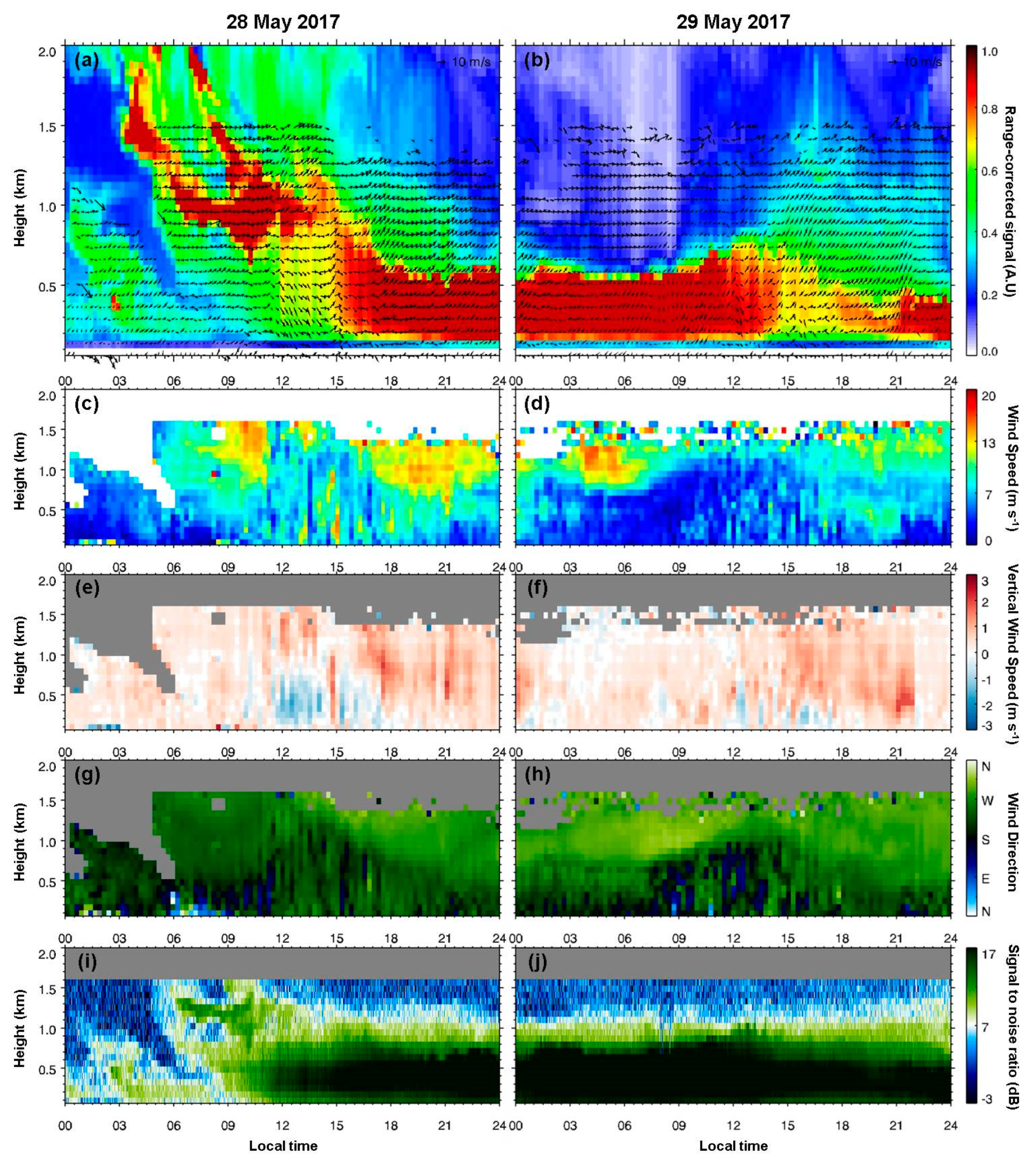
Figure 7 shows the profiles of wind speed and direction from 28–29 May 2017, which differs from Figure 6 in temporal variation. Winds were more influenced by the synoptic weather pattern than thermally induced convection. Wind shear was clearly observed during this period, and westerlies were consistent throughout the whole period. Wind speed did not show drastic changes throughout the day, as evidenced by the average wind speed of 7.59 ± 3.07 m s−1 between 10:00 and 20:00 local time and 7.11 ± 3.55 m s−1 during the rest of the day. This observation differs greatly from the temporal variation of wind speed in the case in Figure 6. Unlike in Figure 6, the WDL detection range did not show a large temporal variation, especially during 29 May 2017, and the WDL provided close-to-consistent observations up to its maximum detection range during the entire day. This was possible due to a thick aerosol layer that was advected from around 1.5 km at 5:00 local time down to the surface (Figure 7a). A downdraft observed at noon on 28 May 2017 coincided with the sudden downward entrainment of the aerosol layer, gradually increasing the aerosol loading at the near surface (Figure S1). On the other hand, a slight reduction in surface aerosol concentration was induced by the strong updrafts at 15:00 local time on 29 May 2017. However, it is difficult to conclude that downdrafts result in aerosol entrainment to the surface and updrafts in diffusion, because even for the days given in Figure 7, the relationship between vertical wind and aerosol movement is not consistent. Further studies with more observation data are needed for a comprehensive understanding of the mechanism between aerosol advection and winds within the PBL.

4. Conclusions

In this study, two wind retrieval methods, namely, the sine-fitting method and the SVD method, were compared using simultaneous radiosonde soundings as reference data. The sine-fitting method was employed by the instrument manufacturer and independent wind data (wind speed and wind direction) were retrieved by applying the SVD to the radial velocity, lidar elevation, and azimuth angle data. Comparing 17 radiosonde sounding experiments, it was concluded that the sine-fitting method showed better performance with regard to the number of points, but the SVD method resulted in significantly smaller bias and root-mean-square error with radiosonde soundings. Increasing the averaging time interval of the velocity azimuth display scans when using the SVD method resulted in significant improvement of the WDL wind retrieval accuracy. The daily wind profiles observed with the WDL for the two cases, namely, thermally induced boundary layer dynamics (27–28 May 2016) and boundary layer dynamics influenced by the synoptic weather pattern to a greater extent (28–29 May 2017), showed very different characteristics. While the wind speed and wind direction showed large variation throughout the day due to thermally induced flows for the former case, wind profiles were more consistent for the latter. For the case of 28–29 May 2017, in particular, we could define aspects where wind variation affected the advection of aerosols within the PBL. More case studies using the improved WDL wind retrieval method and additional observations will help improve our understanding of winds into the PBL and their effects on aerosol vertical distribution. Such an investigation will also provide valuable information for air quality modeling.

Supplementary Materials

The following are available online at https://www.mdpi.com/2072-4292/10/8/1261/s1, Figure S1: PM10 and PM2.5 surface concentration observed at ground station Dongjak (refer to Figure 1) on 28 and 29 May 2017 (data sourced from www.airkorea.or.kr).

Author Contributions

S.-W.K. and S.P. were primarily responsible for the original idea and experimental design. S.P., S.-W.K., and M.-S.P. conducted the experiments, and C.-K.S. provided several helpful suggestions to improve the quality of the paper.

Funding

This research was funded by the Korea Meteorological Administration Research and Development Program under grant KMI2018-05010. C.-K. Song was supported by the National Strategic Project-Fine Particle of the NRF funded by the Ministry of Science and ICT (MSIT), the Ministry of Environment (ME), and the Ministry of Health and Welfare (MOHW) (grant No. NRF-2017M3D8A1092021).

Conflicts of Interest

The authors declare no conflict of interest.

References

  1. Reitebuch, O.; Strassburger, A.; Emeis, S.; Kuttler, W. Nocturnal secondary ozone concentration maxima analysed by sodar observations and surface measurements. Atmos. Environ. 2000, 34, 4315–4329. [Google Scholar] [CrossRef]
  2. Ouwersloot, H.; Vilà-Guerau de Arellano, J.; Nölscher, A.; Krol, M.; Ganzeveld, L.; Breitenberger, C.; Mammarella, I.; Williams, J.; Lelieveld, J. Characterization of a boreal convective boundary layer and its impact on atmospheric chemistry during HUMPPA-COPEC-2010. Atmos. Chem. Phys. 2012, 12, 9335–9353. [Google Scholar] [CrossRef] [Green Version]
  3. Baker, W.E.; Atlas, R.; Cardinali, C.; Clement, A.; Emmitt, G.D.; Gentry, B.M.; Hardesty, R.M.; Källén, E.; Kavaya, M.J.; Langland, R. Lidar-measured wind profiles: The missing link in the global observing system. Bull. Am. Meteorol. Soc. 2014, 95, 543–564. [Google Scholar] [CrossRef]
  4. Davies, F.; Middleton, D.; Bozier, K. Urban air pollution modelling and measurements of boundary layer height. Atmos. Environ. 2007, 41, 4040–4049. [Google Scholar] [CrossRef]
  5. Zhang, D.-L.; Zheng, W.-Z. Diurnal cycles of surface winds and temperatures as simulated by five boundary layer parameterizations. J. Appl. Meteorol. 2004, 43, 157–169. [Google Scholar] [CrossRef]
  6. Barlow, J.F.; Dunbar, T.M.; Nemitz, E.G.; Wood, C.R.; Gallagher, M.W.; Davies, F.; O’Connor, E.; Harrison, R.M. Boundary layer dynamics over London, UK, as observed using Doppler lidar during REPARTEE-II. Atmos. Chem. Phys. 2011, 11, 2111–2125. [Google Scholar] [CrossRef] [Green Version]
  7. Emeis, S.; Schäfer, K. Remote Sensing Methods to Investigate Boundary-layer Structures relevant to Air Pollution in Cities. Bound.-Lay. Meteorol. 2006, 121, 377–385. [Google Scholar] [CrossRef]
  8. Emeis, S.; Schäfer, K.; Münkel, C. Surface-based remote sensing of the mixing-layer height–A review. Meteorol. Z. 2008, 17, 621–630. [Google Scholar] [CrossRef] [PubMed]
  9. Strauch, R.G.; Merritt, D.A.; Moran, K.P.; Earnshaw, K.B.; Kamp, D.V.D. The Colorado Wind-Profiling Network. J. Atmos. Ocean. Technol. 1984, 1, 37–49. [Google Scholar] [CrossRef]
  10. Weitkamp, C. Lidar: Range-Resolved Optical Remote Sensing of the Atmosphere; Springer Science & Business: New York, NY, USA, 2006; Volume 102, ISBN 0387251014. [Google Scholar]
  11. Pearson, G.; Davies, F.; Collier, C. Remote sensing of the tropical rain forest boundary layer using pulsed Doppler lidar. Atmos. Chem. Phys. 2010, 10, 5891–5901. [Google Scholar] [CrossRef] [Green Version]
  12. Bingöl, F.; Mann, J.; Foussekis, D. Conically scanning lidar error in complex terrain. Meteorol. Z. 2009, 18, 189–195. [Google Scholar] [CrossRef]
  13. Päschke, E.; Leinweber, R.; Lehmann, V. An assessment of the performance of a 1.5 μm Doppler lidar for operational vertical wind profiling based on a 1-year trial. Atmos. Meas. Tech. 2015, 8, 2251–2266. [Google Scholar] [CrossRef] [Green Version]
  14. Sroga, J.T.; Eloranta, E.W.; Barber, T. Lidar Measurement of Wind Velocity Profiles in the Boundary Layer. J. Appl. Meteorol. (1962–1982) 1980, 19, 598–605. [Google Scholar] [CrossRef] [Green Version]
  15. Werner, C. Doppler Wind Lidar. In Lidar: Range-Resolved Optical Remote Sensing of the Atmosphere; Weitkamp, C., Ed.; Springer: New York, NY, USA, 2005; pp. 325–354. ISBN 978-0-387-25101-1. [Google Scholar]
  16. Browning, K.; Wexler, R. The determination of kinematic properties of a wind field using Doppler radar. J. Appl. Meteorol. 1968, 7, 105–113. [Google Scholar] [CrossRef]
  17. Kim, S.-W.; Berthier, S.; Raut, J.-C.; Chazette, P.; Dulac, F.; Yoon, S.-C. Validation of aerosol and cloud layer structures from the space-borne lidar CALIOP using a ground-based lidar in Seoul, Korea. Atmos. Chem. Phys. 2008, 8, 3705–3720. [Google Scholar] [CrossRef] [Green Version]
  18. Park, M.-S. Overview of Meteorological Surface Variables and Boundary-Layer Structures in the Seoul Metropolitan Area during the MAPS-Seoul Campaign. Aerosol Air Qual. Res. 2018, in press. [Google Scholar] [CrossRef]
  19. Pearson, G.; Davies, F.; Collier, C. An Analysis of the Performance of the UFAM Pulsed Doppler Lidar for Observing the Boundary Layer. J. Atmos. Ocean. Technol. 2009, 26, 240–250. [Google Scholar] [CrossRef]
Figure 1. Geological location of the Gwanak, Jungnang, and Dongjak sites, and topography of the Seoul metropolitan area.
Remotesensing 10 01261 g001
Figure 2. Examples of 15-min-averaged wind profiles using the sine-fitting method and singular value decomposition (SVD) method and radiosonde soundings. The colors indicate profiles retrieved from velocity–azimuth display (VAD) scans of different averaging time periods. LST stands for local standard time.
Remotesensing 10 01261 g002
Figure 3. (a) Number of data points, (b) bias, and (c) root-mean-square error (RMSE) between radiosonde and wind Doppler lidar wind speed from the sine-fitting method and for variation in the averaging time interval in the SVD method.
Remotesensing 10 01261 g003
Figure 4. Examples of angular distribution of radial velocity from the third gate (approximately 200 m altitude) observed by the wind Doppler lidar during the 15 min after the start of the radiosonde flight. The colored points indicate the initial VAD scan with each color indicating the minute during which the data point was measured (i.e., data points with the same color were measured during the same minute). The black points indicate the 15-min-averaged VAD scan.
Remotesensing 10 01261 g004
Figure 5. Scatter plot of wind speed (left column: a,c) and direction (right column: b,d) from radiosonde soundings (x-axis) and wind Doppler lidar measurements (y-axis), using the sine-fitting method (upper panel: a,b) and the SVD method (lower panel: c,d).
Remotesensing 10 01261 g005
Figure 6. Diurnal variation in the aerosol backscatter range-corrected signal with wind vectors (a,b), wind speed (c,d), vertical wind speed (e,f), wind direction (g,h) and wind Doppler lidar signal-to-noise ratio (i,j) measured during 27 May 2016 (left column) and 28 May 2016 (right column).
Remotesensing 10 01261 g006
Figure 7. Diurnal variation of the aerosol backscatter range-corrected signal with wind vectors (a,b), wind speed (c,d), vertical wind speed (e,f), wind direction (g,h), and wind Doppler lidar signal-to-noise ratio (i,j) measured during 28 May 2017 (left column) and 29 May 2017 (right column).
Remotesensing 10 01261 g007
Table 1. Instrument specifications of the scanning Doppler light detection and ranging (lidar, LR-S1D2GA).
Wavelength1.55 μm
Pulse repetition rate16 kHz
Doppler velocity range−30 m s−1–30 m s−1
Range resolution30 m, 75 m, 150 m (user-defined)
Average power7 W (@ 75 m resolution)
Table 2. Technical specifications of the scanning Doppler lidar.
Scanning ModePlan Position Indicator (PPI)
Sampling frequency16 kHz
Scanning speed1° s−1
Range resolution75 m
Zenith angle80°
Azimuth angle−90°–90°

