Radar Scatter Decomposition to Differentiate between Running Ice Accumulations and Intact Ice Covers along Rivers

Abstract

For ice-jam flood forecasting it is important to differentiate between intact ice covers and ice runs. Ice runs consist of long accumulations of rubble ice that stem from broken up ice covers or ice-jams that have released. A water wave generally travels ahead of the ice run at a faster celerity, arriving at the potentially high flood–risk area much sooner than the ice accumulation. Hence, a rapid detection of the ice run is necessary to lengthen response times for flood mitigation. Intact ice covers are stationary and hence are not an immediate threat to a downstream flood situation, allowing more time for flood preparedness. However, once ice accumulations are moving and potentially pose imminent impacts to flooding, flood response may have to switch from a mitigation to an evacuation mode of the flood management plan. Ice runs are generally observed, often by chance, through ground observations or airborne surveys. In this technical note, we introduce a novel method of differentiating ice runs from intact ice covers using imagery acquired from space-borne radar backscatter signals. The signals are decomposed into different scatter components—surface scattering, volume scattering and double-bounce—the ratios of one to another allow differentiation between intact and running ice. The method is demonstrated for the breakup season of spring 2018 along the Athabasca River, when an ice run shoved into an intact ice cover which led to some flooding in Fort McMurray, Alberta, Canada.

1. Introduction

Ice-jam releases can be quite detrimental to flood-prone areas for a number of reasons. The water wave and running ice accumulation created by the release of impounded water and ice can travel at high velocities of up to almost 11 m/s [1,2] leading to high rates of water level rise with very little notice in high flood risk areas. This is particularly difficult for emergency measure coordination when evacuations in such high flood hazard areas are required. The extra water and ice can also exasperate an existing ice-jam situation by adding ice to the ice-jam volume and flow to increase backwater staging. The momentum of the additional water and ice flow can shove into the existing jam to thicken its cover, which in turn increases the jam’s underside roughness to augment backwater staging. Hence, from an ice-jam flood forecasting perspective, it is important to distinguish between ice upstream of a flood-prone area, that is; (i) intact or (ii) running and accompanying a water wave. Intact ice provides some delay in the time when the ice can potentially become a hazard to the downstream-lying areas of flood risk. The running ice generally stems from broken up ice covers or ice-jam releases. The arrival of the ice accumulation in the flood-prone area is more imminent, reducing the time for flood preparedness and potentially having to switch from flood mitigation activities to an evacuation mode of the flood management plan.

Much work has already been carried out to study the behaviour of ice-jam releases and their effects on existing downstream ice covers, ice-jams and open water stretches. Earlier work established empirical criteria to determine the onset of breakup. Guo [3] successfully used the shear stress of the water flow on the ice cover as a criterion for ice cover breakup. Ettema [4] emphasised the important role confluences play as conducive locations for the jamming and release of ice accumulations. Jasek [5] studied ice-jam releases and their effects along the Porcupine and Yukon rivers in the Yukon Territory of Canada. Shen and Liu [6] studied a rare occurrence of an ice-jam on the Shokotsu River in Japan showing that, not only the rapid flow increase from snowmelt but also geomorphological characteristics at the jam location (rapid reduction in slope and width in the flow direction) were responsible for the mechanical breakup that led to jamming of the resulting ice accumulations. Beltaos and Burrell [7,8] studied field data of ice-jam release waves (javes) on the Little Southwest Miramichi, Restigouche and Saint John rivers in New Brunswick to characterise parameters describing the waveforms. Once the parameters have been calibrated, particularly celerities of the leading edge and crest of the waves, flow velocities, discharges and shear stress induced by the javes can be quantified. Kowalczyk Hutchinson and Hicks [2] and She et al. [9] investigated ice-jam releases along the Athabasca River and provided a protocol for the collection of data required for numerical modelling of ice-jam releases. Nafziger et al. [10] studied the effects of ice runs in sequence along the Hay River and paid particular attention to the changes in shape and celerity of water wave and ice run hydrographs. Beltaos [1] investigated ice-jam release waves in the lower Mackenzie River and the upper channels of the river’s delta. Shen et al. [11] applied the model DynaRICE, a two-dimensional flow and ice model, to study the behaviour of ice-jam releases and highlighted the importance of upstream flood waves in instigating ice-jam releases. Kolerski and Shen [12] applied the model to calculate bed shear stress during the release of an ice-jam along the St. Clair River, flowing from the Laurentian great lake Lake Huron to Lake St. Clair. They established that there needs to be a substantial increase in the stress for backwater from ice-jamming and subsequent ice-jam release to occur. Knack et al. [13] applied the same model to the Saint-John River in New Brunswick, Canada, to simulate ice cover breakup and found that much of the breakup occurrences along that river are due to accumulations from upstream ice-jam release surges.

In general, several insights can be gleaned and summarized from these studies in regard to an ice-jam flood forecasting context. Firstly, both water waves and ice runs disperse as they travel along the river. The celerity of the water waves is generally faster than those of the ice runs. This adds complexity to flood forecasting efforts since the rising flood waters precede the arrival of the running ice accumulation. The ice run can be readily detected by observations from the ground or aerial surveys, which do not provide enough warning for the arrival of the water wave. Secondly, fluvial geomorphology has a marked influence on the hydrograph shapes and travel as they advance along the river. For instance, ice run surface concentrations and celerities can increase when the ice accumulation passes through a width constriction along the river and river segments that are deep. As the slope of the river decreases, as in delta channels, breakup of the ice cover is mostly caused by upstream-originating ice-jam release waves. Thirdly, there are differences in the surge behaviours depending if they are impeded (the water and ice flow into an existing ice cover or jam) or unimpeded (the water and ice flow along an open stretch of water). Stalled jams, when the flow of ice temporarily stops or slows down allowing backwater staging to increase before releasing again, can accentuate wave peaks potentially resulting in more havoc in the flood-prone area.

All of these studies relied on ground observations, either through inspection, recording instrumentation, photography (trail cameras), aerial surveys (helicopter or fixed-wing airplane), numerical modelling and space-borne remote sensing. The use of satellite imagery to distinguish between intact and running ice has thus far not been reported in the scientific literature.

In this technical note, we introduce a novel methodology of differentiating between the two ice covers, intact and running ice, using microwave backscatter signals from the RADARSAT-2 sensor. The sensor allows the transmission and receiving of electromagnetic waves polarised in both horizontal (H) and vertical (V) planes, from which four different transmission-receiving combinations (quad-polarisation) can be acquired; HH, HV, VH, and VV. The four backscatter signals (HH, HV, VH, and VV) can be decomposed into surface backscattering, volume scattering, and double bounce scattering components using the Freeman–Durden decomposition technique [14]. The Freeman–Durden decomposition is a physical-based model, first developed to estimate the contribution of volume scattering from randomly oriented dipoles, surface scattering of first-order Bragg surface, and double bounce scattering, to the total backscatter [14]. The backscattering components of C-band SAR (Synthetic Aperture Radar) images decomposed using the Freeman–Durden decomposition technique have been used to distinguish between solid and macro-porous ice covers and monitoring river ice cover development along the Slave River [15,16]. According to the authors’ knowledge, no other applications of this method to river ice has been reported in the scientific literature, since it has only recently been applied in the river ice context.

For snow-covered freshwater ice covers, double bounce scattering of SAR–freshwater ice interaction is typically in a small and negligible magnitude. For a SAR sensor with specific SAR parameters (i.e., wavelength and look angle), the surface scattering component is controlled by the roughness and the permittivity (Ɛ) contrast between air (Ɛ~1.0), snow (dry snow: Ɛ: 1.0–2.0), ice (Ɛ~3.7), and water (Ɛ~80), and volume scattering is controlled by the physical properties of snow and ice [17,18]. For an interface with similar magnitude of surface roughness, the larger the permittivity contrast, the larger the reflection coefficient at the interface thus resulting in the larger surface backscattering. The discussion in this paper is based on C-band SAR. Dry snow on the ice surface and the air/snow interface have limited contribution to the backscattering decomposition components of C-band SAR image [19,20]. The surface scattering component of SAR–freshwater ice interactions is mainly determined by the effective roughness of the ice–water interface due to the large dielectric contrast of water and ice, followed by the roughness of the snow–ice–water interface [15,18,20,21]. However, the ice–water interface in a river typically is smoothed due to thermal erosion and thus has limited contribution to the surface scattering. In addition, the C-band radar pulse usually cannot penetrate the ice layers of consolidated ice covers and reach the bottom ice because of the absorption and reflection of different mediums with variable permittivity [21]. Hence, the main contributor of surface scattering of river ice is the roughness of the snow–ice interface. When the surface of ice covers becomes wet during the ice breakup season, the increased dielectric contrast between the snow/air–ice interface would result in the increase in surface backscattering. The volume scattering is mainly determined by physical properties of ice covers, which mainly refer to the inclusions, including air bubbles, dead vegetation, and sediments in ice covers, as well as the porosity of ice covers.

Ice runs typically have a wetter surface and a greater porosity than intact ice covers, and therefore ice runs are expected to have higher surface scattering due to the increased dielectric contrast of the snow/air–ice interface and a larger volume scattering because of increased porosity of ice covers. Hence, in this paper, we apply the surface backscattering and volume backscattering of the Freeman–Durden decomposition, and the ratio of volume and surface scattering to differentiate between intact and running ice to provide valuable information for ice-jam predictions in a flood forecasting context.

2. Study Site

The study site is the Athabasca River near Fort McMurray, Alberta, Canada extending approximately 200 km from the mouth of the House River to approximately 15 km downstream of the Clearwater River mouth (see Figure 1). The reach upstream of Fort McMurray is relatively steep (slope ≈ 0.001), narrow (width of 150–250 m) and sinuous, interspersed with many rapids making this stretch conducive to the generation of a thick consolidated ice cover during river freeze-up and to sequences of ice-jamming and release during ice cover breakup. The fluvial geomorphology changes abruptly at Fort McMurray when the river flows into a reach with a bed that is much flatter (slope ≈ 0.0003) and wider (width = 300–700 m). Although less sinuous, this reach is interlaced with islands providing many sites for the arrest of ice flow and the formation of ice-jams. The inflow from the Clearwater River tributary in this area also provides an additional source of ice and water. However, the tributary also buffers flood staging when Athabasca River water backs up into the Clearwater River when flood waves and ice runs flow along the Athabasca River through and past the Fort McMurray area. This buffering can slow down the flood wave and ice run enough to allow ice to jam downstream of the Clearwater River mouth, exasperating backwater staging. The rising water levels also extend upstream along the Clearwater River to pose a flood hazard to the downtown area of Fort McMurray.

Ice cover breakup monitoring is carried out every spring by scientists and engineers from Alberta Environment and Park’s (AEP) River Forecasting Centre. Important Athabasca River gauges are used to track water level elevations, shown in Figure 1, including the one just upstream of Grand Rapids, those just downstream of Crooked and Cascade rapids and the one at the Athabasca River Bridge. Other gauges along the Athabasca River are usually available, but failed during the spring of 2018 breakup period, hence are not shown in Figure 1.

Trail cameras, aerial surveys and satellite images are also used to monitor the progression of spring breakup. Products from RADARSAT-2 and SENTINEL-1 satellite imagery provide classifications of the ice cover into sheet or rubble ice, both intact ice covers, and open water stretches [22]. However, a classification between intact ice covers and moving/floating ice that constitute ice runs is not yet integrated in the classification protocol. Oftentimes, the satellite imagery is not available because acquisitions conflict with other end users or due to long revisit intervals, hence some optical satellite sensors such as the Terra and Aqua sensors of the MODIS (Moderate Resolution Imaging Spectroradiometer) mission have been drawn upon to fill in time gaps. Optical imagery is limited, though, to cloud-free and daytime observations. It is hoped that with the launch of the Radarsat Constellation Mission (RCM) in February 2019, a more reliable and frequent imagery source will be made available which is desperately needed in an ice-jam flood forecasting context. The reader is referred to Lindenschmidt et al. [23] for an example of the requirements of an ice-jam flood forecasting system.

3. Methods

To differentiate the ice runs from intact ice, the Freeman–Durden decomposition [14] was applied to the SQ5W RADARSAT-2 images acquired at 06:57 on 26 April 2018. The incidence angle of a SQ5W RADARSAT-2 image ranges from 22.5° to 26.0° and the nominal range resolution is between 20.6 and 23.6 m. We used the Freeman–Durden decomposition because it has performed well in monitoring ice cover development [16]. Mermoz et al. [21] also applied a similar but mathematics-based decomposition approach, the Cloude–Pottier decomposition method [24], to determine ice thicknesses. The scattering mechanism of surface scattering and volume scattering on differentiating the ice covers of ice runs and intact ice covers dominated by consolidated ice are proposed in Figure 2.

A mask was applied to isolate the river. Prior to decomposition, the SQ5W image was orthorectified in PCI Geomatica 2017 using the Radar-Specific Model and the ASTER Global Digital Elevation Model Version 2 (GDEM V2). The pixel size of the image was resampled to 25 m using the nearest neighbour method and Sigma Nought radiometric correction was also applied. The orthorectified and radiometrically corrected image was then despeckled by applying a boxcar filter within a 5 × 5 pixel moving window using the PoLSAR Boxcar Filter in the Focus Module of PCI Geomatica 2017. Finally, the asymmetric covariance matrix of the despeckled SQ5W image was converted to a symmetric covariance matrix and the Freeman–Durden decomposition was applied to the symmetric covariance matrix to decompose the total power to the contribution of surface scattering, volume scattering and double bounce in the Focus Module of PCI Geomatica 2017.

The decomposed volume, surface backscattering, and their ratio were used to differentiate ice covers of ice runs from intact ice covers. MODIS images (used for validation of ice cover conditions when cloud free), aerial photographs, and gauge hydrographs at the Grand Rapids, Crooked Rapids, Cascade Rapids, and Fort Murray Bridge, taken in the ice breakup time of the winter of 2017–2018 were used to support the analysis. A flowchart has been provided in Figure 3.

4. Ice Cover Breakup of Spring 2018

On 24 April 2018, the ice cover along the river stretch of interest was intact, as evidenced in the Terra MODIS imagery acquired on that day (figure not shown). The following day, deterioration of the ice cover was quite advanced with some areas exhibiting the opening up of water leads in the ice cover, particularly near rapids.

As reported by Alberta Parks and Environment [25,26] and referring to the ice map in Figure 4, some sections along the intact ice cover (orange) between Grand Rapids and Crooked Rapids had moved and broken up resulting in accumulations of rubble ice at the downstream ends of open water stretches (dark blue in Figure 4) approximately 1 to 3 km in length. Some stretches where the ice had broken but not moved were flooded with water (light blue in Figure 4) or had open leads (Figure 5b). Some ice accumulations had resulted in the formation of small ice-jams approximately 2 km in length (red in Figure 4, Figure 5a). The ice cover between Crooked Rapids and Fort McMurray remained intact (Figure 5c). The river downstream of the Clearwater River mouth was open for approximately 15 km (Figure 5d).

Some movement of the ice cover became first evident in the water level hydrographs recorded at Grand Rapids at 10:15 on 25 April 2018 (Figure 6a). Breakup of the ice cover was first recorded at Grand Rapids at midnight, during the night from 25 to 26 April 2018 (Figure 6b). The wave of this breaking front propagated downstream to arrive at the Crooked Rapids gauge 7 hours later (Figure 6c), at the Cascade Rapids gauge (Figure 6d) and at the bridge gauge (Figure 6e), all during the same morning. The breaking front wave tripped the ice movement indicators at 07:00 and 07:45, respectively at Crooked and Cascade rapids (Figure 6f,g). The RADARSAT-2 image was acquired three minutes before ice movement was recorded at Crooked Rapids, dedicating Crooked Rapids to a threshold location, upstream of which the ice was running and downstream of which the ice cover was still intact. The breakup reached the Fort McMurray bridge at approximately 10:00 (Figure 6e) with a large amount of ice and water being forced into the Fort McMurray area. Celerities of this impeded breaking front (propagating downstream into an intact ice cover) decreased in the downstream direction from an average of 3.87 m/s between Grand and Crooked rapids, 3.67 m/s between Crooked and Cascade rapids, and 3.12 m/s between Cascade Rapids and the bridge.

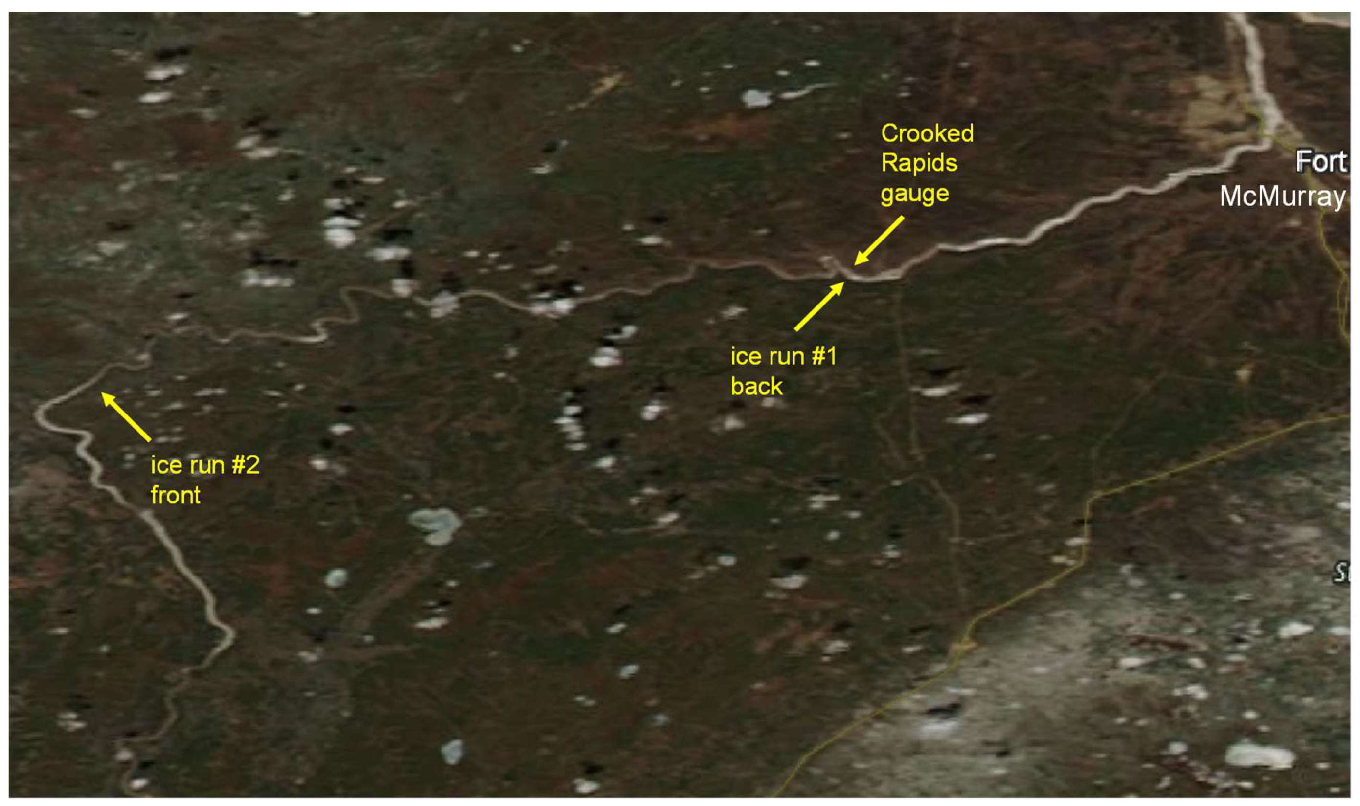
An ice run that began far upstream of our study site, indicated as ice run #2 in Figure 7 and Figure 8, arrived at the Crooked Rapids gauge at 18:30 on 26 April 2018 (Figure 6h) and progressed further downstream, arriving at the Cascade Rapids gauge approximately a half hour later (Figure 6i). The celerity of this unimpeded ice run front (propagating downstream into open water or water with free-floating ice) between these two gauges averaged 4.85 m/s, which is faster than the previously propagating impeded breaking front. This ice run added water and ice (Figure 6j) to the already high water and ice flows at the bridge.

Both ice movement indicators at Crooked and Cascade rapids recorded movement of the ice run for approximately 26.5 h, until 09.35 and 10:00 on 27 April 2018 at the respective gauges (Figure 6k,l).

5. Results and Discussion

The top panel of Figure 9 shows longitudinal profiles of the surface scattering, volume scattering, and double bounce averaged along the course of the river. The double bounce was very small in relation to the other two scatter components. Surface scattering overpowered volume scattering for most of the stretch, in particular the stretch with intact ice. However, in the stretch with running ice, upstream of the Crooked Rapids gauge (35 to 48 river km), the volume scatter did appear to approach the same power contribution as surface scattering. This was more differentiated in the ratio volume scattering/surface scattering as shown in the bottom panel of Figure 9. Intact ice has a very low volume to surface scattering ratio, while an ice run has a much larger volume/surface ratio.

The power contribution of the volume scatter did become substantial downstream of the bridge where the local ice cover may have broken up and formed consolidated ice covers. Unfortunately, photographs were not taken during this time to provide evidence, however, a stretch of open water between −3.5 and −5 river-km did point to an area where the ice cover had broken up from which the rubble ice would had to have travelled downstream to shove into the downstream ice cover to form a jam between −5 and −8 river-km. Water levels recorded at the bridge (Figure 6m) did indicate some staging at the time the RADARSAT-2 image was acquired. For open water, almost all of the transmitted microwaves were reflected and scattered forward from the water surface, hence little scatter components remained.

Some higher volume scatter relative to the surface scatter was shown a few kilometres upstream of the bridge, between 4 and 6 river-km (top panel of Figure 9), with a relative strong volume scatter/surface scatter ratio (bottom panel of Figure 9). This may be due to some breakup of the local ice cover, however, this was difficult to verify since no photographic evidence was available for this stretch at that time.

Figure 10 shows a spatial representation of the decomposed scatter components at Crooked Rapids. This area represents the transition from running ice and intact ice. Again, the double bounce signal was minute and need not to be shown in the figure. However, both the surface and volume scatter components, respectively the top and middles panels of the figure, had higher values in the ice run stretch (upstream of the gauge) than the intact ice stretch (downstream of the gauge), which coincides with the results shown in Figure 10. More distinction in the transition from running to intact ice can be seen in the map of the volume scatter/surface scatter ratio, shown in the bottom panel of Figure 10. The running ice will be more porous and wetter, hence exhibit more surface scattering, whereas the intact ice will retain more volume scattering due to its continuous, solid medium.

The river reach with ice runs showed higher volume and surface scattering and a larger volume to surface scattering ratio than the reach covered by intact ice. The dramatically increased volume scattering of ice runs is probably attributed to the interactions of radar pulse between adjacent broken ice in ice runs (increased porosity of ice runs). However, numerical modelling and more images at ice breakup are needed to confirm this finding in the future. For intact ice, volume scattering mainly stems from the inclusions (e.g., air bubbles, sediments, and air bubbles) in ice covers [19,21]. The amount of such inclusions determines the contribution of volume scattering to the total backscattering. The large surface scattering was attributed to the rough air–ice interface [17], while the contribution of the ice–water interface in a high flow river channel was negligible because the bottom of ice is typically smooth in a river with high water flow due to the thermal erosion. In this regard, the larger surface scattering of ice runs may result from the increased surface roughness, compared to intact ice. In addition, broken ice covers of ice runs tend to have a wetter surface, compared to the intact ice covers, which would also account for the higher surface scattering as a result of an increased dielectric contrast of the air–ice interface.

Applying Freeman–Durden decomposition to C-band quad-pol RADARSAT-2 images has demonstrated great potential to differentiate ice runs from intact ice in this study. Nevertheless, further research or observation data is needed to investigate the sources of the high volume scattering and large ratio of volume to surface scattering near and downstream of the bridge.

6. Conclusions

Using the Freeman–Durden decomposition method, intact ice and running ice were successfully differentiated from quad-pol RADARSAT-2 imagery. This novel method of using space-borne imagery to provide wider coverage of ice characteristics along rivers can be very useful in an ice-jam flood forecasting context. Characterising the difference between running and stationary ice covers helps determine the potential timing of the arrival of water and ice run waves which can lead to ice-jam backwater staging and flooding in high flood risk areas. This methodology will also refine an ice-jam flood forecasting approach using a stochastic modelling approach first applied to the town of Fort McMurray in the spring of 2018. A second attempt of stochastic ice-jam flood forecasting is planned for the spring breakup of 2019 and it is hoped that differentiating between running ice and intact ice can help better quantify the volumes of ice available for ice-jamming in the town.

References

- Beltaos, S. Hydrodynamic properties of ice-jam release waves in the Mackenzie Delta, Canada. Cold Reg. Sci. Technol. 2014, 103, 91–106. [Google Scholar] [CrossRef]
- Kowalczyk Hutchinson, T.; Hicks, F. Observations of ice jam release waves on the Athabasca River near Fort McMurray, Alberta. Can. J. Civ. Eng. 2007, 34, 473–484. [Google Scholar]
- Guo, Q. Applicability of criterion for onset of river ice breakup. J. Hydraul. Eng. 2002, 128, 1023–1026. [Google Scholar] [CrossRef]
- Ettema, R.; Muste, M.; Kruger, A. Ice jams in river confluences. In Cold Regions Research and Engineering Laboratory Report 99-6; U.S. Army Corps of Engineers: Hanover, NH, USA, 1999. [Google Scholar]
- Jasek, M. Ice jam release surges, ice runs, and breaking fronts: Field measurements, physical descriptions, and research needs. Can. J. Civ. Eng. 2003, 30, 113–127. [Google Scholar] [CrossRef]
- Shen, H.T.; Liu, L. Shokotsu River ice jam formation. Cold Reg. Sci. Technol. 2003, 37, 35–49. [Google Scholar] [CrossRef]
- Beltaos, S.; Burrell, B. Determining ice-jam-surge characteristics from measured wave forms. Can. J. Civ. Eng. 2005, 32, 687–698. [Google Scholar] [CrossRef]
- Beltaos, S.; Burrell, B. Field measurements of ice-jam-release surges. Can. J. Civ. Eng. 2005, 32, 699–711. [Google Scholar] [CrossRef]
- She, Y.; Andrishak, R.; Hicks, F.; Morse, B.; Stander, E.; Krath, C.; Keller, D.; Abarca, N.; Nolin, S.; Nzokou Tanekou, F.; et al. Athabasca River ice jam formation and release events in 2006 and 2007. Cold Reg. Sci. Technol. 2009, 55, 249–261. [Google Scholar] [CrossRef]
- Nafziger, J.; She, Y.; Hicks, F. Celerities of waves and ice runs from ice jam releases. Cold Reg. Sci. Technol. 2016, 123, 71–80. [Google Scholar] [CrossRef]
- Shen, H.T.; Gao, L.; Kolerski, T.; Liu, L. Dynamics of Ice Jam Formation and Release. J. Coast. Res. 2008, 52, 25–31. [Google Scholar] [CrossRef]
- Kolerski, T.; Shen, H.T. Possible effects of the 1984 St. Clair River ice jam on bed changes. Can. J. Civ. Eng. 2015, 42, 696–703. [Google Scholar] [CrossRef]
- Knack, I.M.; Shen, H.T. A numerical model study on Saint John River ice breakup. Can. J. Civ. Eng. 2018, 45, 817–826. [Google Scholar] [CrossRef]
- Freeman, A.; Durden, S.L. A three-component scattering model for polarimetric SAR data. IEEE Trans. Geosci. Remote Sens. 1998, 36, 963–973. [Google Scholar] [CrossRef]
- Lindenschmidt, K.-E.; Das, A.; Chu, T. Air pockets and water lenses in the ice cover of the Slave River. Cold Reg. Sci. Technol. 2017, 136, 72–80. [Google Scholar] [CrossRef]
- Lindenschmidt, K.-E.; Li, Z. Monitoring river ice cover development using the Freeman–Durden decomposition of quad-pol RADARSAT-2 images. J. Appl. Remote Sens. 2018, 12, 026014. [Google Scholar] [CrossRef]
- Ulaby, F.T.; Moore, R.K.; Fung, A.K. Microwave Remote Sensing: Active and Passive. Volume 1—Microwave Remote Sensing Fundamentals and Radiometry, Addison-Wesley, Reading, Massachusetts; Artech House Publishers: Norwood, MA, USA, 1981. [Google Scholar]
- Gunn, G.E. Re-Evaluating Scattering Mechanisms in Snow-Covered Freshwater Lake Ice Containing Bubbles Using Polarimetric Ground-Based and Spaceborne Radar Data. Ph.D. Thesis, University of Waterloo, Waterloo, ON, Canada, 2015. [Google Scholar]
- Gherboudj, I.; Bernier, M.; Leconte, R. A backscatter modeling for river ice: Analysis and numerical results. IEEE Trans. Geosci. Remote Sens. 2010, 48, 1788–1798. [Google Scholar] [CrossRef]
- Atwood, D.K.; Gunn, G.E.; Roussi, C.; Wu, J.; Duguay, C.; Sarabandi, K. Microwave backscatter from Arctic lake ice and polarimetric implications. IEEE Trans. Geosci. Remote Sens. 2015, 53, 5972–5982. [Google Scholar] [CrossRef]
- Mermoz, S.; Allain-Bailhache, S.; Bernier, M.; Pottier, E.; Van Der Sanden, J.J.; Chokmani, K. Retrieval of river ice thickness from C-band PolSAR data. IEEE Trans. Geosci. Remote Sens. 2014, 52, 3052–3062. [Google Scholar] [CrossRef]
- Puestow, T.; Cuff, A.; Richard, M.; Tolszczuk-Leclerc, S.; Proulx-Bourque, J.-S.; Deschamps, A.; van der Sanden, J.; Warren, S. The River Ice Automated Classifier Tool (RIACT). CGU HS Committee on River Ice Processes and the Environment. In Proceedings of the 19th Workshop on the Hydraulics of Ice Covered Rivers, Whitehorse, YT, Canada, 9–12 July 2017. [Google Scholar]
- Lindenschmidt, K.-E.; Carstensen, D.; Fröhlich, W.; Hentschel, B.; Iwicki, S.; Kögel, M.; Kubicki, M.; Kundzewicz, Z.W.; Lauschke, C.; Łazarów, A.; et al. Development of an ice-jam flood forecasting system for the lower Oder River—Requirements for real-time predictions of water, ice and sediment transport. Water 2019, 11, 95. [Google Scholar] [CrossRef]
- Cloude, S.; Pottier, E. An entropy based classification scheme for land applications of polarimetric SAR. IEEE Trans. Geosci. Remote Sens. 1997, 35, 68–78. [Google Scholar] [CrossRef]
- Alberta Environment and Parks. 2018 Athabasca River Report No. 5 – River Ice Observation Report. River Forecasting Centre, Alberta Environment and Parks, 25 April 2018. Available online: http://environment.alberta.ca/forecasting/RiverIce/pubs/rfs_ice_observation_report_20180425_173000.pdf (accessed on 2 February 2019).
- Alberta Environment and Parks. 2018 Athabasca River Report No. 5 – River Ice Observation Map. River Forecasting Centre, Alberta Environment and Parks, 25 April 2018. Available online: https://environment.alberta.ca/forecasting/RiverIce/pubs/rfs_ice_observation_map_20180425_174500.pdf (accessed on 2 February 2019).
Figure 1.
Athabasca River near Fort McMurray, Alberta.
Figure 2.
The scheme of surface and volume scattering of fully polarimetric SAR (Synthetic Aperture Radar) images for differentiating (a) intact ice covers and (b) ice runs (adapted from Gherboudj et al. [19]).
Figure 3.
The procedures of image processing and differentiation of ice covers of ice runs and intact ice covers.
Figure 4.
Ice map of the Athabasca and Clearwater rivers near Fort McMurray from 25 April 2018 (data source: [26]).
Figure 5.
(a) Small ice-jam downstream of Grand Rapids; (b) Open lead in intact ice cover at Crooked Rapids; (c) Intact ice extending 6 km upstream of bridges; (d) Intermittent ice cover downstream of Clearwater River mouth. (source: [26]).
Figure 6.
Gauges from hydrographs during the April 2018 breakup event.
Figure 7.
MODIS Terra image acquired 26 April 2018 11:35 MST.
Figure 8.
MODIS Aqua image acquired 26 April 2018 13:23 MST.
Figure 9.
Longitudinal profile of averaged backscatter components (top panel) and ratio of volume scattering/surface scattering (bottom panel).
Figure 10.
Surface scatter (top panel), volume scatter (middle panel) and volume scatter/surface scatter ratio (bottom panel) (RADARSAT-2 Data and Products © MacDonald, Dettwiler and Associates Ltd—All Rights Reserved. RADARSAT is an official trademark of the Canadian Space Agency).
© 2019 by the authors. Licensee MDPI, Basel, Switzerland. This article is an open access article distributed under the terms and conditions of the Creative Commons Attribution (CC BY) license (http://creativecommons.org/licenses/by/4.0/).
Share and Cite
MDPI and ACS Style
Lindenschmidt, K.; Li, Z. Radar Scatter Decomposition to Differentiate between Running Ice Accumulations and Intact Ice Covers along Rivers. Remote Sens. 2019, 11, 307. https://doi.org/10.3390/rs11030307
AMA Style
Lindenschmidt K, Li Z. Radar Scatter Decomposition to Differentiate between Running Ice Accumulations and Intact Ice Covers along Rivers. Remote Sensing. 2019; 11(3):307. https://doi.org/10.3390/rs11030307
Chicago/Turabian StyleLindenschmidt, Karl–Erich, and Zhaoqin Li. 2019. "Radar Scatter Decomposition to Differentiate between Running Ice Accumulations and Intact Ice Covers along Rivers" Remote Sensing 11, no. 3: 307. https://doi.org/10.3390/rs11030307
Note that from the first issue of 2016, this journal uses article numbers instead of page numbers. See further details here.