Competition and Burn Severity Determine Post-Fire Sapling Recovery in a Nationally Protected Boreal Forest of China: An Analysis from Very High-Resolution Satellite Imagery

Abstract

Anticipating how boreal forest landscapes will change in response to changing fire regime requires disentangling the effects of various spatial controls on the recovery process of tree saplings. Spatially explicit monitoring of post-fire vegetation recovery through moderate resolution Landsat imagery is a popular technique but is filled with ambiguous information due to mixed pixel effects. On the other hand, very-high resolution (VHR) satellite imagery accurately measures crown size of tree saplings but has gained little attention and its utility for estimating leaf area index (LAI, m²/m²) and tree sapling abundance (TSA, seedlings/ha) in post-fire landscape remains untested. We compared the explanatory power of 30 m Landsat satellite imagery with 0.5-m WorldView-2 VHR imagery for LAI and TSA based on field sampling data, and subsequently mapped the distribution of LAI and TSA based on the most predictive relationships. A random forest (RF) model was applied to assess the relative importance and causal mechanisms of spatial controls on tree sapling recovery. The results showed that pixel percentage of canopy trees (PPCT) derived from VHR imagery outperform all Landsat-derived spectral indices for explaining variance of LAI (R²_VHR = 0.676 vs. R²_Landsat = 0.427) and TSA (R²_VHR = 0.508 vs. R²_Landsat = 0.499). The RF model explained an average of 55.5% (SD = 3.0%, MSE = 0.382, N = 50) of the variation of estimated LAI. Understory vegetation coverage (competition) and post-fire surviving mature trees (seed sources) were the most important spatial controls for LAI recovery, followed by burn severity (legacy effect), topographic factors (environmental filter) and nearest distance to unburned area (edge effect). These analyses allow us to conclude that in our study area, mitigating wildfire severity and size may increase forest resilience to wildfire damage. Given the easily-damaged seed banks and relatively short seed dispersal distance of coniferous trees, reasonable human help to natural recovery of coniferous forests is necessary for severe burns with a large patch size, particularly in certain areas. Our research shows the VHR WorldView-2 imagery better resolves key characteristics of forest landscapes like LAI and TSA than Landsat imagery, providing a valuable tool for land managers and researchers alike.

1. Introduction

Wildfire has been well recognized as a crucial process governing the dynamics of forest structure, composition and function in boreal forests [1,2]. Severe burns can cause abrupt changes to forest ecosystem by killing living plants, consuming organic matter, and altering biophysical environments [3,4,5]. In general, forest ecosystems are resilient and able to recover key functional and compositional attributes after disturbances [6,7,8]. However, the resilience of boreal forests is decreasing due to a misalignment between changing fire regimes and vulnerable ecosystem states [9,10,11]. Biome transitions in boreal forests, including shifts from forests to treeless steppes and an increase in deciduous trees, are thought to be exacerbated by changing fire regimes [12,13,14,15]. In addition, both fire frequency and severity in boreal ecosystems is predicted to increase in the future [16,17,18,19]. Research on the spatial controls of forest restoration post-fire is essential for understanding how boreal ecosystems respond to changing fire regimes and advancing ecologically sound policies in boreal fire management and restoration.

Tree sapling regeneration is strongly correlated to the future successional trajectory of burned forests and thus can be used to anticipate future compositional and structural dynamics [20,21]. Structural attributes of regeneration observed in the field, such as abundance, biomass, and species composition, can be used to determine the strength of post-fire forest recovery [21,22,23,24]. Field-based inventory approaches can provide first-hand information, but this is a labor-intensive and time-consuming process with limited utility for long-term monitoring over a broad spatial scale. On the other hand, remote sensing is a novel and cost-effective technique for monitoring forest ecosystems [25], as well as for evaluating fire-related characteristics such as burn severity [26,27], burned area [28], and monitoring post-fire vegetation recovery [29,30,31].

Satellite imagery for monitoring post-fire vegetation dynamics assumes that the remotely sensed surface reflectance can capture spectral signal variations that correspond to vegetation recovery. Vegetation indices were designed to reflect vegetation photosynthesis and were widely accepted as surrogates of canopy attributes, biomass, or tree coverage across global forest ecosystems [30,32]. However, spectral variation as exhibited in satellite imagery is not a biophysical parameter that can precisely characterize structure or function of forest ecosystems [33]. Forest recovery is typically described ambiguously in terms of changes in vegetation index or greenness in remote sensing literatures, however little attention has been paid to investigate whether such remotely sensed spectral information can reflect key forest structures in newly established boreal forest stands [34,35]. On the other hand, structural attributes rather than spectral variations are the critical indicators of forest ecosystem functions (i.e., carbon sequestration and water budgets) [36,37], and are thus more important for assessing forest recovery for management and scientific perspectives.

Tree sapling abundance (TSA), the number of tree saplings per unit area, is a crucial attribute of the post-fire forest stands as it determines the future successional trajectory of forests [38,39]. Burned areas with high TSA have a higher possibility of developing as forests through succession and recovery processes, while burned areas with few tree saplings may take a longer time to approach canopy closure. The spatial distribution of TSA is thus a critical reference for directing artificial management measures that aim to promote forest restoration post-fire. Leaf area index (LAI) is another structural attribute with critical importance to forest productivity and biomass accumulation through influencing forest canopy photosynthesis [40,41]. LAI can be measured rapidly in the field and is one of the few forest structures that is well-linked to optical remote sensing at various spatial scales [42,43].

Spatially monitoring these two structural attributes is essential for understanding the functional dynamics of post-fire forest ecology but presents a challenge for traditional remote sensing approaches. In post-fire landscapes, tree sapling distribution usually exhibits a high degree of heterogeneity as a result of interactions among seed availability (legacy effects), filter effects from environmental factors, inter- and intraspecific competition and edge effects [23,44]. Previous studies aimed at disentangling these effects were dependent on field investigations but very high-resolution (VHR) satellite imagery, which can provide fine details of post-fire landscapes (<1 m), is a promising approach that has not previously been utilized for tree saplings. The high resolution of VHR imagery is significant in allowing for accurate assessment of tree sapling crown size, but very few studies have investigated the utility of VHR imagery for monitoring forest structural attributes in newly reestablished stands.

Based on this, we sought to address the following questions: (1) How do the performances of VHR and Landsat imagery differed for delineating the spatial distribution of TSA and LAI in the early post-fire landscape; (2) which spatial controls (interspecific competition, legacy effects, environmental filters or edge effects) are most important in the recovery of LAI and TSA post-fire; and (3) how do these spatial control factors influence (inhibiting or facilitating) spatial distribution of LAI and TSA post-fire?

2. Materials and Methods

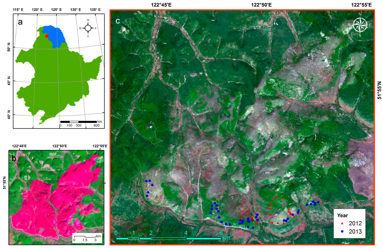
2.1. Study Area

The study was conducted in Huzhong National Natural Reserve of Great Xing’an Mountains (Figure 1), where primary forests are well protected since all logging has been prohibited since 1958. In this area, post-fire forests follow a natural recovery process and successional trajectory without artificial seeding or plantation. A strict ban on logging of natural forests has been enforced across the Great Xing’an Mountains since April 2014, thus historical fires in the nature reserve will provide valuable insight for understanding how resilient this forest is in responding to wildfire and for refining post-fire management practices. The particular fire (Lat/Lon: 122°50′E, 51°53′N) we studied was ignited by lightning on 17 June 2000 and lasted for seven days [45]. It burned an area approximately 7735 ha, most of which was moderate-high severity with high tree mortality rates [26,39].

The pre-fire forests were dominated by Dahurian larch (Larix gmelinii), a deciduous conifer, and a few deciduous broadleaf species of birch (Betula platyphylla) and aspen (Populus davidiana and Populus suaveolens) [46]. Some evergreen conifers including Scotch pine (Pinus sylvestris var. mongolica) and Korean spruce (Picea koraiensis) were also sparsely distributed. The understory layer was the primary fuel bed and source of ladder fuels [45], which consisted of evergreen shrubs (e.g., Pinus pumila, Ledum linnaeus and Vaccinium vitisidaea), deciduous shrubs (e.g., Betulafruticosa and Rhododendron dauricum linnaeus) and some herbaceous plants (e.g., Chamaenerion angustifolium, Carex appendiculata and Rubus linnaeus) that varied with edaphic and topographic conditions [47]. This area has a relatively short growing seasons (150 days) and frost-free period (~80–100 days), with a mean annual temperature of approximately −4.7 °C and mean annual precipitation of about 460 mm [26]. The topography is mountainous with elevation ranges from 760 m to 1300 m.

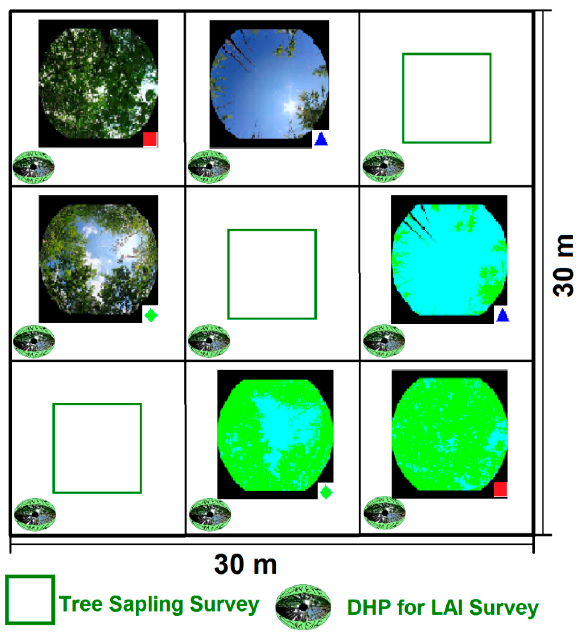
2.2. Field Data Collection

For field data collection, we focused our attention on two structural attributes of post-fire vegetation, TSA and LAI, which can be easily evaluated in the field. In summers of 2012 and 2013, our field crews collected 70 plots of sapling inventory data for both TSA and LAI (Figure 1), with plot size set to 30 m × 30 m in order to match the spatial resolution of Landsat imagery and to minimize potential scale issues. This will improve the accuracy of linkage between in situ measurement and Landsat spectral properties. All sites were at least 150 m from roads to eliminate edge effect and were selected according to severity and topographic positions. Within each plot, we set three 5 m × 5 m quadrants along the diagonal (~42 m) to survey sapling stems with a height greater than 1.5 m (Figure 2). We did not distinguish between tree species (although most were white birch and larch) as they were not differentiable in VHR imagery due to very similar spectral signature and highly mixed in situ. All saplings were counted based on the number of stems (>1.5 m) because asexual resprouting of white birch is common. TSA was calculated as the mean number of saplings and was normalized to saplings per hectare.

LAI was measured using a digital hemispherical photography (DHP) system using a Canon EOS 60D Digital Single Lens Reflex camera and a Sigma 8-mm F3.5 EX DG Fisheye lens. We followed the user manual of CAN-EYE software (Version 6.3.3, National Institute of Agronomical Research, Toulouse, France) to calibrate our DHP system and derive the parameters for establishing the projection functions [48]. Using a 1920 × 1280 pixels parameter for digital photograph, our calibration process generated accurate projection functions that are comparable with results as shown in user manual (see Appendix A). The DHP system was installed to a tripod with a fixed 0.70 m height. Within each sampling plot, we took nine upward digital photographs distributed as shown in Figure 2. Following the recommendation of the user manual, the limit of the circle of interest was set as 60° in CAN-EYE software to avoid mixed pixels effects in the blended photograph edges. Other input parameters were set as either default values or derived from photographs automatically. Given this procedure, dead standing stems with large diameter had the potential to influence the LAI estimation, so we manually masked them during the image process in CAN-EYE software to reduce the overestimation. The canopy of surviving trees was retained, however, because their greenness was involved in Landsat spectral signals and not possible to isolate.

2.3. Remote Sensing for Estimating Vegetation Coverage

2.3.1. Remote Sensing Data Process

The cloud-free WorldView-2 (DigitalGlobe. Inc., Herndon, VA, USA, Figure 1) image was acquired on 1 June 2014 at 2 m spatial resolution including four multispectral bands (Blue 450–510 nm; Green 510–580 nm, Red 705–745 nm, and near infrared (NIR) 860–1040 nm) and 0.5 m spatial resolution for panchromatic band (450–800 nm). We used the Pan Sharpening toolbox in ENVI 5.3 software (Harris Geospatial Solution. Inc., Washington, DC, USA) to perform image fusion, and improved the spatial resolution of multispectral bands to 0.5 m. The WorldView-2 imagery had been geo-spatially projected using the Universal Transverse Mercator (UTM) coordinate system based on WGS-84 ellipsoid with a nominal positioning accuracy of 3.5 m. It is accurately overlapped with Landsat imageries, which have 30-m spatial resolution.

To produce time-synchronous comparisons between Landsat and field survey, the spectral indices were extracted according to the year when the TSA and LAI data were collected in the field. In addition, we used the same field data for the Landsat-derived indices of 2014 in order to form an unbiased comparison with WorldView-2 data. We obtained 8 Landsat-5 TM, Landsat-7 ETM+, and Landsat-8 OLI surface reflectance images (path-row: 122/24 and 121/24, time: 2010, 2012–2014) from the EROS Science Processing Architecture (ESPA) system of the USGS (

Table 1. Detailed information of Landsat scenes. Invalid pixels are cloud, shadow and null value pixels.

Satellite	Sensor	Acquisition Date	Path-Row	Percentage of Invalid Pixels	Usage
Landsat-5	TM	5 September 2011	122-24	3.6%	Reference Image
Landsat-7	ETM+	30 August 2012	122-24	21.7%	Spectral Indices
Landsat-7	ETM+	8 September 2012	121-24	33.1%	Spectral Indices
Landsat-8	OLI	25 August 2013	122-24	36.8%	Spectral Indices
Landsat-8	OLI	3 September 2013	121-24	13.3%	Spectral Indices
Landsat-8	OLI	21 August 2014	121-24	33.2%	Spectral Indices
Landsat-7	ETM+	29 August 2014	121-24	35.0%	Spectral Indices
Landsat-7	ETM+	5 September 2014	122-24	31.0%	Spectral Indices

). Atmospheric and topographic correction had been carried out for these before distribution. Due to the lack of cloud-free days over the study area during the time periods assessed, we used “cloud masking” to remove cloud and shadow pixels [49], and then carried out image mosaic to fill data-gap for each year. Although the intra-annual Landsat imageries have very close observation dates, we still applied the iteratively re-weighted multivariate alteration detection (IR-MAD) approach to minimize spectral inconsistency among Landsat sensors [50,51]. The Landsat-5 imagery of 2011 was used as the reference imagery for band-by-band radiometric normalization. The mean correlation coefficients (for 6 bands) of four target imageries were each higher than 0.95, indicating good performance of IR-MAD for radiometric normalization.

2.3.2. Landsat-Derived Spectral Indices

Vegetation indices developed from remote-sensed Red and NIR bands, such as the Normalized Differenced Vegetation Index (NDVI), are often used as indicators of vegetation recovery in many forest ecosystems [31]. But saturation issues with vegetation indices are widely reported [34,52], especially in areas covered with dense vegetation, which may limit the strength of vegetation indices for detecting structural changes related to forest recovery [30]. Spectral indices derived from the shortwave infrared (SWIR) bands, which are sensitive to water content in vegetation foliage, are proving to be good indicators of post-fire recovery in many forest ecosystems [34,53,54]. In addition, components of Tasseled Cap (TC) transformation (i.e., brightness, greenness and wetness) and their modified spectral indices are also commonly used for monitoring forest disturbance and forest recovery [55]. Different indices may provide different perspectives of forest recovery. Therefore, it is critical to elucidate which Landsat-derived spectral indices have the feasibility to depict post-fire tree sapling attributes in our ecosystem. Such efforts can be helpful to provide an in-depth understanding of what remote sensing indices mean in the field. To comprehensively investigate the performance of Landsat-derived spectral indices on estimating TSA and LAI, we calculated nine commonly-used spectral indices (

Table 2. Formulas of nine Landsat-derived spectral indices. Spectral Index Abbreviation: NDVI—Normalized Difference of Vegetation Index; EVI—Enhanced Vegetation Index [56]; SAVI—Soil Adjusted Vegetation Index [52]; MSAVI—Modified Soil Adjusted Vegetation Index [52]; NBR—Normalized Burn Ratio [54]; NDMI—Normalized Difference Moisture Index [57]; TCA—Tasseled Cap Angle [55]; TCW—Tasseled Cap Wetness. Note: spectral bands are different between Landsat5/7 and Landsat 8.

Spectral Index	Spectral Index
$NDVI=\frac{{\rho }_{NIR}-{\rho }_{Red}}{{\rho }_{NIR}+{\rho }_{Red}}$	$NBR=\frac{{\rho }_{NIR}-{\rho }_{SWIR2}}{{\rho }_{NIR}+{\rho }_{SWIR2}}$
$EVI=\frac{2.5\times ({\rho }_{NIR}-{\rho }_{Red})}{{\rho }_{NIR}+6\times {\rho }_{Red}-7.5\times {\rho }_{Blue}+1}$	$NDMI=\frac{{\rho }_{NIR}-{\rho }_{SWIR1}}{{\rho }_{NIR}+{\rho }_{SWIR1}}$
$EVI2=\frac{2.5\times ({\rho }_{NIR}-{\rho }_{Red})}{{\rho }_{NIR}+2.4\times {\rho }_{Red}+1}$	$TCA=\arctan (\frac{T{C}_{Greeness}}{T{C}_{Brightness}})$
$SAVI=\frac{{\rho }_{NIR}-{\rho }_{Red}}{1.5\times \left({\rho }_{NIR}+{\rho }_{Red}+0.5\right)}$	$\begin{array}{ll}TCW=0.1446\times & {\rho }_{Blue}+0.1761\times {\rho }_{Green}+0.3322\times {\rho }_{Red}\\ & +0.3396\times {\rho }_{NIR}-0.621\times {\rho }_{SWIR1}\\ & -0.4186\times {\rho }_{SWIR2}-3.3828\end{array}$
$MSAVI=0.5\times (2\times {\rho }_{NIR}+1-\sqrt{{\left(2\times {\rho }_{NIR}+1\right)}^2-8\times \left({\rho }_{NIR}-{\rho }_{Red}\right)})$

) to analyze their explanatory strength.

2.3.3. Image Textures of WorldView-2 Imagery

The WorldView-2 has limited spectral bands that cannot sufficiently support to calculate much spectral indices, but it offers image textures to improve the land cover mapping [58,59] and estimation of forest structures [60,61], yet its performance in estimating attributes of sapling tree was not verified. Using the panchromatic band of WorldView-2 imagery, we calculated 13 image texture variables, which consist of five occurrence measures and eight co-occurrence measures. The occurrence measures directly use the number of occurrences of each gray level within a given moving window for calculating summaries of statistics (i.e., Range, Mean, Variance, Entropy and Skewness). The co-occurrence measures are second-order statistical calculations involving the spatial relationships among neighboring pixels. The grey level co-occurrence matrix, which is a function of both the angular relationship and distance between a central pixel and its neighboring pixels, was used to calculate eight statistical measures including mean, variance, homogeneity, contrast, dissimilarity, entropy, angular second moment (ASM), and correlation.

Calculation of image texture is influenced by the window size as it determines the number of surrounding pixels. Wood, et al. [62] suggested that a small window size for image texture analysis may best match the spatial scale at which the forest structure varies. We tested three kinds of window size, including 5 × 5, 15 × 15 and 25 × 25, but did not find notable differences for subsequent analysis. We chose a 5 × 5 window size for all texture variable calculations because it matches the spatial size of a single tree sapling and since it was the least costly in computing time. We did not calculate image texture for Landsat imagery because our field plots had identical spatial size with Landsat pixel, which means the measured TSA and LAI can only reflect within-pixel (30 m) variations. All image texture variables were computed using ENVI 5.3 software (Harris Geospatial Solution. Inc., Herndon, VA, USA).

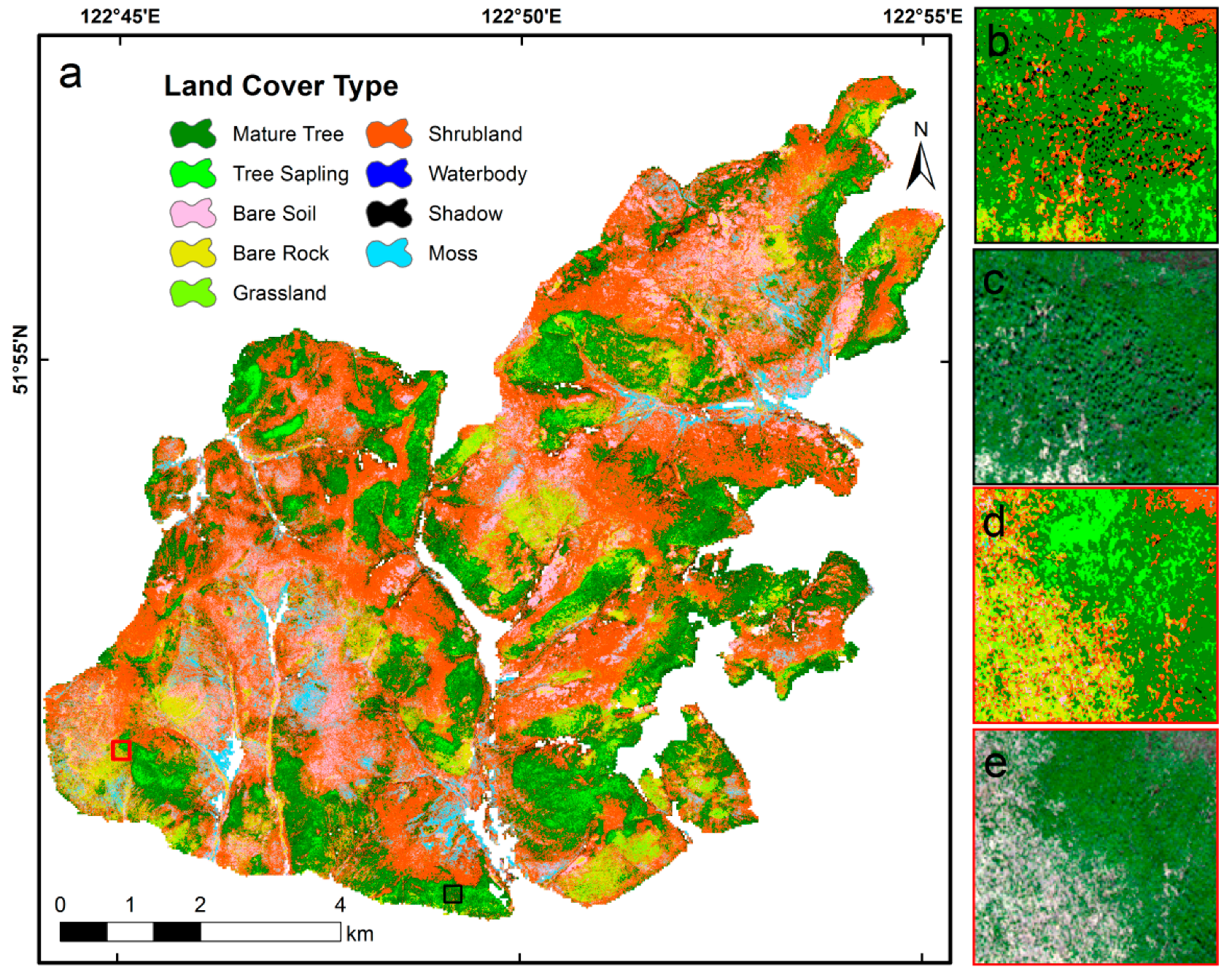
2.3.4. Land Cover Mapping of WorldView-2 Imagery

We used the per-pixel classification method to obtain the land cover information from the 0.5 m WorldView-2 imagery. According to our field knowledge and visual interpretation of the imagery, we used a classification scheme consisting of 9 popular objects in the field during the preliminary analysis. We used the support vector machine (SVM) approach to carry out the land cover classification. The SVM is a supervised classifier that has been widely applied for land cover and land use mapping through the local to global spatial scales [63,64]. Training pixels were selected with very high confidence based on our knowledge. We chose over 3000 training pixels for each land cover type in order to provide sufficient model training and avoid overfitting problem [65]. We calculated the Jeffries–Matusita distance (JMD) to evaluate the separability of training pixels, defined as:

$$JM{D}_{xy}=2\left(1-e^{-B}\right)$$

where B is the Bhattacharyya distance, which is usually used for indicating dissimilarity between two distributions:

$$B=\frac{1}{8}{\left(x-y\right)}^t{\left(\frac{\sum x+\sum y}{2}\right)}^{-1}\left(x-y\right)+\frac{1}{2}ln\left(\frac{\left|\frac{\sum x+\sum y}{2}\right|}{\sqrt{\left|\sum x\right|\times \left|\sum y\right|}}\right)$$

In this equation, x and y are two vectors of spectral and textural signatures and $\sum x$ and $\sum y$ are covariance matrix of x and y respectively [66]. The JMD will be close to 2 when spectral and textural signatures of two classes are completely different (high separability), and close to 0 when spectral and textural signatures are identical (low separability).

Classification accuracy was evaluated based on additional pixels (~1000 pixels for each class) that were independently selected from the training pixels. Using the confusion matrix approach [67], we calculated the Cohen’s Kappa coefficient to evaluate overall classification accuracy, and used the omission error and commission error to evaluate accuracy of individual class. The ability to distinguish tree saplings from the surviving trees was desired to refine our research. However, we found low separability between these two classes (

Table 3. Description of predictors used in random forest models.

Predictor	Category	Description
dNBR	Legacy effect	Indicator of burn severity, calculated based on bi-temporal difference of NBR. Higher dNBR values represent higher tree mortality and more combustion of surface organic matters.
Shadow	Legacy effect	Surrogate amount of surviving trees post-fire. This is derived from the 0.5 m land cover map of WorldView-2. Higher shadow coverage indicates more surviving trees (and likely higher seed availability).
Elevation	Topography filter	Altitude of a given site.
TPI	Topography filter	Topographic position index. A positive TPI value indicates a higher altitude than neighborhood pixels, while a negative TPI value indicates a lower altitude than surrounding areas. A TPI value of 0 indicates a flat area or an area near mid-slope.
TWI	Topography filter	Topographic wetness index. TWI values typically range from 3 to 30. Higher TWI values indicate high soil moisture potential.
Solar radiation	Topography filter	Incoming solar radiation from a raster surface during the growing season. Higher values indicate higher exposure to solar radiation. Southern-facing slopes usually have higher solar radiation.
Understory coverage	Competition	Percentage of pixels classified as understory (grasslands and shrublands) in land cover map of WorldView-2 for each 30 m × 30 m site. Higher understory coverage indicates more space occupied by understory plants. Understory plants do not include tree sapling here.
Nearest Distance	Edge Effect	The nearest distance to unburned areas. It reflects the potential of a given site to receive seed source from unburned areas with proximity to unburned forests indicating a higher likelihood of receiving seeds.

). We also found low separability between grasslands and shrublands and therefore combined those classes for the further analysis (but reported accuracies evaluated based on the nine-class scheme).

2.4. Statistical Analysis

2.4.1. Compare Performance of Landsat and WorldView-2 on Predicting TSA and LAI

To match the spatial size of field data, we conducted spatial aggregation to obtain statistical measures for information derived from WorldView-2 data. For the land cover map, we used a moving window (60 × 60 pixels), whose spatial size is consistent with spatial resolution of Landsat imagery, to compute the percentage of pixels that were classified as the canopy trees (i.e., tree saplings and mature trees), denoted as PPCT. For image texture, we conducted spatial aggregation to obtain the mean value for each texture variable. Given high collinearity among image texture variables, pairwise Pearson correlation coefficients (r) calculated from the “Hmisc” package in R 3.4.1 (R Development Core Team 2017, Boston, MA, USA) were used as the criteria based on randomly sampled 300 pixels. We used a forward stepwise method combined with variance inflation factors (VIF) functions in the “car” package to drop variables with high collinearity by applying a stringent threshold of 3, following recommendation of Zuur, et al. [68]. Landsat spectral indices often show collinearity as their computation may use the same spectral bands. Because of this we only retained two co-occurrence texture variables (i.e., mean and ASM) and one occurrence texture variable (i.e., Entropy) as they represented low correlations (|r| < 0.50). We retained all spectral indices for the further analysis to allow us to investigate the usage of a spectral index in monitoring post-fire vegetation dynamics.

The presence of spatial autocorrelation in dependent variables may violate the assumption that all observations are independent, which will inflate the significance and affect the coefficient estimates. Using functions in the “ape” package [69], we calculated the Moran’s I index to examine spatial autocorrelations in our measured TSA and LAI respectively. Moran’s I is similar to a correlation coefficient ranging between −1 and 1. Higher positive values indicate greater similarity, while lower negative values indicate stronger dissimilarity. Autocorrelation was found significant at α < 0.05 level, but very weak for both TSA (Moran’s I = 0.18) and LAI (Moran’s I = 0.20). It suggested our field observations on TSA and LAI have low spatial dependence, and the subsequent analysis will not be strongly influenced by spatial autocorrelation.

The coefficient of determination (R²) was used to evaluate the explanatory power of remotely sensed variables for variations of field-measured TSA and LAI. Because the LAI is partially determined by tree density, it is not surprising that our LAI data represented very high correlation (r = 0.783, p < 0.01) with TSA data. We retained both variables for the remote sensing analysis as they reflect different perspectives of forest structure and may be sensitive to different spectral bands. Before parameterizing the regression model, we applied the Shapiro-Wilk test and histogram approach to detect whether the normality assumption is violated [70]. If the null hypothesis (i.e., samples came from a normally distributed population) was rejected at α < 0.05 level, we applied logarithm transformation to mitigate skew. Homogeneity of variance was evaluated using the Fligner–Killeen test [71]. The test results indicated that the null hypothesis (i.e., all populations variances are equal) was not violated in any regression model. Outliers (Cook’s distance greater than four times of the mean) were detected and removed. The Landsat indices and WorldView-2 variables with the highest R2 were used to predict TSA and LAI through the post-fire landscape.

2.4.2. Evaluation of Relative Importance Using Random Forest Model

We used the random forest (RF) model in the “randomForest” package to evaluate the relative importance of spatial controls on determining TSA and LAI. The RF model is a machine learning algorithm with advantages for dealing with nonlinear relationships, multi-collinearity, and complex interactions without imposing assumptions on data distribution [72]. Based on a bootstrap subsampling (bagging) scheme, the RF model can generate multiple regression trees with low variance that can be combined for an accurate prediction. The best split of node is chosen from the random subsets of predictor variables to ensure that all predictors are tested. For each individual tree, the remaining (i.e., out-of-bag, OOB) data that not drawn into training subset is used for unbiased model validation [73]. We used the variance explained (R²) to evaluate the goodness of fit of RF model for training data. It is calculated based on the internal OOB error rate in terms of mean of squared residuals (MSE):

$$MSE=n^{-1}{\displaystyle \sum }_1^n{(y_i-{\widehat{y}}_i^{OOB})}^2$$

where ${\widehat{y}}_i^{OOB}$ is the average of the OOB predictions for observation i. The R² is calculated as:

$${\mathrm{R}}^2=\frac{MSE}{{\widehat{\sigma }}_y^2}$$

The most important variable will cause highest degradation on model fit when it is omitted.

Predictors were spatial variables representing gradients of burn severity, topography and understory vegetation abundance (Table 3). Burn severity was evaluated based on a quadratic correlation model (R² = 0.856), which was developed from the difference between the normalized burned ratio (dNBR) and field-sampled severity measures [26]. We applied a 30 m resolution digital elevation model (DEM) to generate topographic variables reflecting elevation, topographic relief, topographic wetness, and the total solar radiation of growing season (April to October). Understory vegetation abundance was derived from WorldView-2 land cover map. Similar to PPCT, we calculated the coverage of understory vegetation (i.e., shrubland and grassland) using a 30 m × 30 m moving window aggregation approach. We also found that the shadow pixels largely reflected mature trees in our WorldView-2 imagery. We used the coverage of tree shadow as a surrogate to represent the number of surviving mature trees post-fire. This is similar to Berner, et al. [74], who applied the tree shadow coverage as a surrogate of tree biomass. To understand the edge effects of unburned areas on post-fire recovery, we also calculated the nearest distance to the edge of unburned area as a predictor. The remote sensed TSA and LAI were used as the response variables for two RF models respectively. We generated random samplings based on a 150 m sampling space to balance the spatial autocorrelation and the maximum sampling number (~500 points). To reduce the risk of stochastic errors and create stable model outputs, we carried out 50 RF modeling trials independently and used the average value as the final result.

3. Results

3.1. Accuracy Assessment of WorldView-2 Classification

Relatively high pairwise JMD values (

Table 4. Pairwise Jeffries–Matusita distance (JMD, values within brackets) and confusion matrix for evaluating intra-classes separability and classification accuracies respectively. The bold represents the number of verified samples.

Class	Mature Tree	Tree Sapling	Bare Soil	Bare Rock	Grass-Land	Shrub-Land	Water Body	Shadow Area	Moss
Mature Tree	958	671			0	0		16
Tree Sapling	(1.83)	342
Bare Soil	(2.00)	(2.00)	919		1	59	1
Bare Rock	(2.00)	(2.00)	103 (1.99)	1029
Grassland	(1.97)	6 (2.00)	3 (1.99)	12 (1.99)	403	10
Shrubland	42 (1.98)	1 (2.00)	6 (1.95)	(2.00)	661 (1.46)	960			43
Water Body	(2.00)	(2.00)	(2.00)	(2.00)	(2.00)	(2.00)	1082	109
Shadow Area	(1.99)	(2.00)	(2.00)	(2.00)	(1.98)	(2.00)	(1.86)	908
Moss	(2.00)	(2.00)	(1.97)	(2.00)	(2.00)	4 (2.00)	(2.00)	(2.00)	1000

) indicated very high spectral dissimilarity among the most of land cover classes. The overall accuracy of classification was 81.3% and the Cohen’s Kappa coefficient was 0.790. Mature trees had strong spectral similarity with tree saplings, resulting in a high rate of commission errors (41.6%) for mature tree classification and high omission error (66.5%) for tree sapling classification. Similarly, spectral separability between shrublands and grasslands was also relatively low, preventing us from distinguishing the two classes in subsequent analyses. Mature trees and tree saplings together occupied about 23.6% of the total burned area, while shrublands and grasslands occupied approximately 51.9% of the total burned area (Figure 3). Bare rock, where vegetation has difficulty establishing, accounted about 10.2% of the total burned area. The remaining 14.3% consisted of bare soil, water bodies, shadow areas and moss.

3.2. Correlations between Remote Sensed Variables and LAI and TSA

All Landsat-derived indices exhibited significant correlations with LAI and TSA (

Table 5. Coefficients of linear regression models for evaluating relationships between remotely sensed variables and leaf area index (LAI) and tree sapling abundance (TSA). Landsat-derived spectral index abbreviations see footnote of Table 2. PPCT—Pixel Percentage of Canopy Tree; Co_Means—Means of Co-occurrence Texture; ASM—Angular Second Moment. RMSE—Root Mean Square Error.

Satellite Imagery	Predictor	LAI €			TSA €
		R2 †	RMSE	Outliers	R2	RMSE	Outliers
Landsat (2010–2013)	EVI €	0.283 **	0.390	3	0.409 **	1.048	3
	EVI2	0.427 **	0.348	4	0.299 **	1.111	3
	MSAVI €	0.282 **	0.396	2	0.251 **	1.188	1
	NBR	0.418 **	0.354	2	0.499 **	0.953	5
	NDMI	0.337 **	0.376	2	0.369 **	1.077	3
	NDVI €	0.376 **	0.367	3	0.316 **	1.13	2
	SAVI €	0.339 **	0.380	2	0.311 **	1.134	2
	TCA	0.405 **	0.354	4	0.351 **	1.076	4
	TCW	0.331 **	0.379	3	0.385 **	1.052	4
Landsat (2014)	EVI	0.171 **	0.412	3	0.173 **	1.196	3
	EVI2	0.377 **	0.359	2	0.322 **	1.09	2
	MSAVI €	0.394 **	0.357	3	0.333 **	1.081	3
	NBR	0.489 **	0.331	5	0.450 **	1.022	3
	NDMI	0.385 **	0.360	3	0.478 **	0.983	4
	NDVI €	0.374 **	0.360	2	0.324 **	1.088	2
	SAVI €	0.368 **	0.362	2	0.304 **	1.105	2
	TCA	0.455 **	0.339	3	0.395 **	1.037	3
	TCW	0.333 **	0.379	3	0.384 **	1.053	4
WorldView-2 (2014)	PPCT €	0.676 **	0.257	4	0.508 **	0.977	2
	Entropy €	0.008	0.437	3	0.038	1.282	3
	Co_Means	0.008	0.437	4	0.002	1.275	3
	ASM €	0.089 *	0.418	4	0.005	1.316	2

^€: Model fits using logarithmic transformation; ^†: Significance code: ** p < 0.01; * p < 0.05.

). In two Landsat cases, the EVI2 (R² = 0.427, RMSE = 0.348, Figure 4a) and NBR (R² = 0.489, RMSE = 0.331, Figure 4d) were found the most explanative Landsat-derived indices for LAI, while the NBR (R² = 0.499, RMSE = 0.953, Figure 4b) and NDMI (R2 = 0.478, RMSE = 0.983, Figure 4e) were the most explanative variables for TSA. Spectral indices derived from SWIR bands (e.g., NBR and NDMI) generally performed better than vegetation indices (e.g., NDVI, EVI, and SAVI). The PPCT variable of WorldView-2 (VHR) explained the highest proportions of variance for LAI (R² = 0.676, RMSE = 0.257, Figure 4c) and TSA (R² = 0.508, RMSE = 0.977, Figure 4f) among all variables, but image texture represented relatively weak correlations (Table 5).

The spatial distributions of LAI (Figure 5a) and TSA (Figure 5b) 14 years post-fire were mapped based on the correlation models with highest R² in Table 5. We found about 51.1% (~4098 ha) of the burned area exhibited high LAI recovery (greater than 1), which corresponded to approximately 10,790~74,380 sapling/ha TSA. About 14.6% (~1169 ha) of the burned area exhibited moderate LAI recovery (between 0.5 and 1) of 4770~10,680 sapling/ha, and approximately 2745 ha of the burned area exhibited recovered poor recovery (LAI < 0.5, and TSA < 4630 sapling/ha).

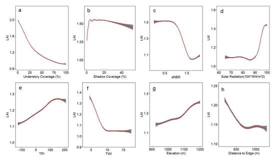
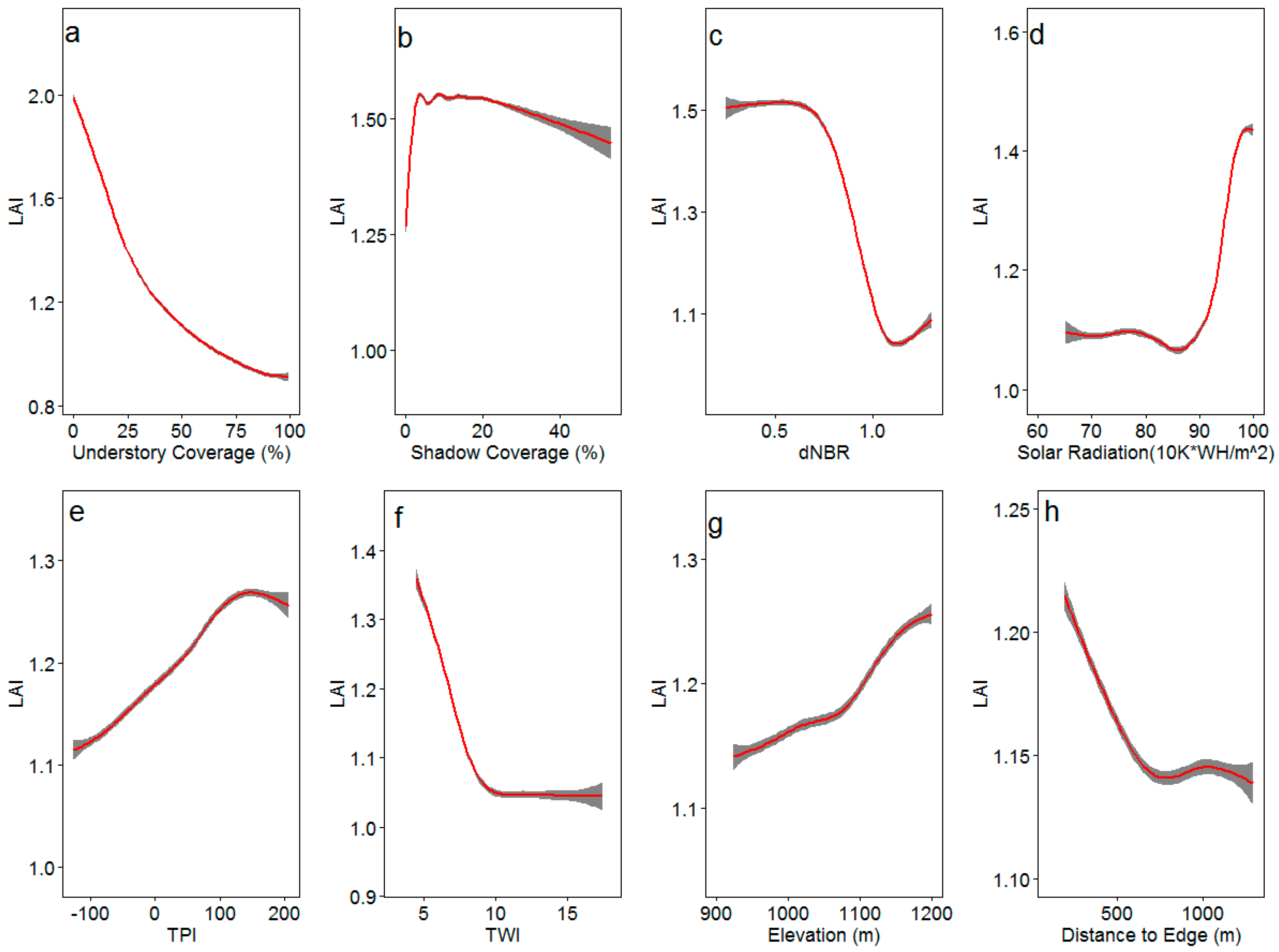
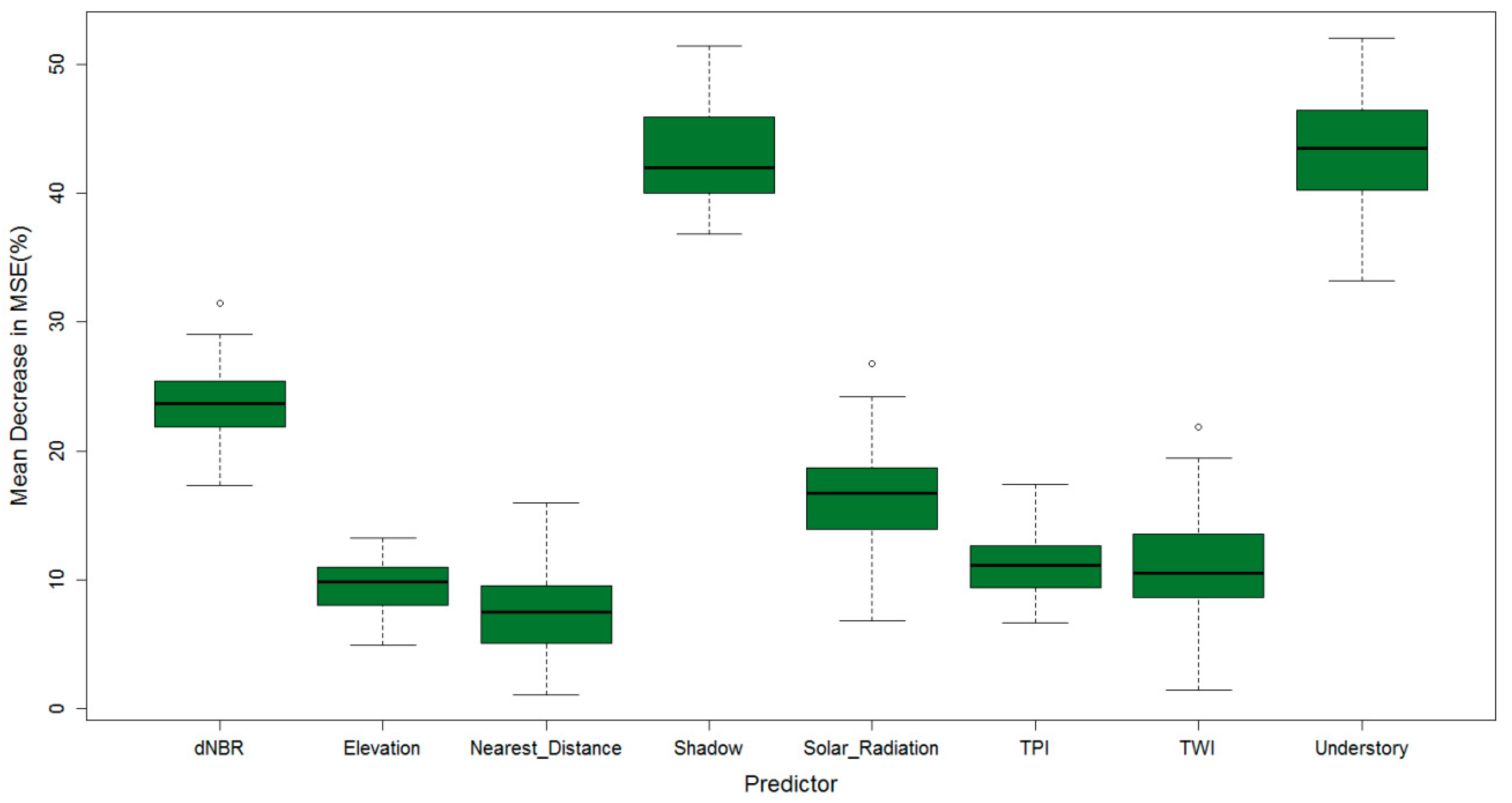
3.3. Relative Importance of Predictors to LAI Recovery

Because WorldView-2 derived PPCT was the most predictive indicator for both LAI and TSA, and LAI and TSA are highly correlated with each other, the RF model produces the same results for both LAI and TSA. Thus we only represented the RF model results for LAI. The 50 RF models explained a maximum of 62.4% (Mean R² = 55.5%, SD = 3.0%, MSE = 0.382, N = 50) of the variation in estimated LAI. The coverage of understory vegetation and shadow pixels were the top-two most important predictor variables, decreasing MSE about 43.3% (SD = 4.6%) and 42.89% (SD = 3.8%) respectively when incorporated in RF models (Figure 6). The dNBR contributed about a 23.4% (SD = 2.9%) decrease in MSE, while contributions of topography variables ranged from 9.6% to 16.7%, followed by Solar Radiation (SD = 3.7%), Topographic Position Index (TPI) (SD = 2.3%), TWI (SD = 3.9%) and Elevation (SD = 2.1%). The edge effect was found to be the least important factor, contributing about a 7.2% (SD = 3.2%) decrease in MSE.

4. Discussion

4.1. Remotely Sensed Estimation of LAI and TSA

Our field investigation suggests that the LAI is highly correlated with TSA in early post-fire landscapes. Given that surveying TSA in the field is time-consuming and labor intensive, utilizing a DHP system can be a more efficient way to monitor post-fire tree sapling recovery. We found that all Landsat-derived spectral indices exhibited statistically significant correlations with both LAI and TSA, but the variance explained was usually less than 50%. EVI2 and NBR were the most predictive spectral indices for LAI and TSA respectively, but we found that NBR performed consistently well for simulating LAI and TSA in two Landsat analysis cases. This suggests that NBR may be the best choice for monitoring post-fire vegetation dynamics in our study area. A similar finding was also reported by Chen, et al. [75], who found that NBR is the most sensitive indicator of post-fire vegetation recovery in the Black Hills National Forest of the USA, suggesting that the value of NBR extends beyond our boreal forest study system. Previous studies have also shown that NBR is better than NDVI for quantifying burn severity [26,76], further supported by Kennedy, Yang and Cohen [54] and White, Wulder, Hermosilla, Coops and Hobart [53], who concluded that the NBR is a very useful indicator for detecting fire disturbance and monitoring post-fire vegetation trajectory.

Although Landsat-derived spectral indices exhibited significant correlations with the LAI and TSA, we found that the WorldView-2 (VHR) imagery performed even better. PPCT had a stronger explanatory power for LAI than for TSA because our DHP measurement of LAI consisted of canopy foliage of both surviving trees and tree saplings. The in-field upward canopy photograph results closely match PPCT derived from WorldView-2 imagery, further confirming the value of this technique. However, PPCT cannot wholly reflect TSA as there were surviving trees that exhibited disproportionately large canopy projection areas in the imagery when compared to tree saplings. The low spectral separability of surviving trees and tree saplings limited the applicability of WorldView-2 imagery for monitoring TSA.

Image textures are commonly used as auxiliary inputs to provide spatial features that spectral information cannot characterize. Many previous studies have reported that including image textures as predictors can improve the estimation of forest structural parameters such as tree diameter [77], stand density [61] and crown diameter [78]. However, image textures did not exhibit strong explanatory power to either LAI or TSA in our study. One reason is that crown shadow is an important factor in representing spatial variation as reflected in the imagery [61]. In contrast to the coarse surface of mature forests, the post-fire landscape where dominated by tree sapling that did not represent very strong shadow effects (contrasts) in the imagery (Figure 3c). In addition, the value of textural features has no explicit relationship to spectral features and the same value of textural attributes may represent very different land surface properties. For example, post-fire landscapes usually exhibit high homogeneity, however similar homogeneity values may be corresponding to different land cover compositions.

4.2. The Response of Forest Recovery to Spatial Controls

We found that including surrogates of intra-specific competition (i.e., understory coverage) and density of surviving trees (i.e., shadow coverage) greatly improved model fit. According to partial dependence curves, we found a negative effect of understory (grass and shrub species) coverage on tree sapling regeneration (Figure 7a). Understory species usually act as pioneers in post-disturbance landscapes and rapidly occupy available spaces and resources. In addition, some understory species are resistant to wildfire and recover rapidly. By comparison, tree saplings may require longer timespans to establish; they will compete with understory species for available resources and may be limited by seed availability.

Tree sapling regeneration (estimated by LAI) is very sensitive to shadow coverage, suggesting that even a few surviving trees can strongly promote post-fire recovery (Figure 7b). The nearest distance to unburned area, which reflects the importance of seed inputs from out of the burned area, significantly impacted LAI recovery with areas near the edge of boundaries having a higher opportunity to receive seeds from unburned areas. Our results showed that edge effects extend for a distance of approximately 700 m for this fire (Figure 7h), which can partially explain why the core area exhibited poor tree recovery. Trees that survive fire are thus critical for supporting reestablishment of tree community post-burn [79,80]. Nonetheless, if the number of surviving trees was over a certain threshold, canopy closure was negatively affected because our study area was dominated by mature larch forests, which have wide tree spacing and relatively open canopies. Surviving trees may prevent the establishment of saplings, likely through resource competition.

Burn severity is often described as a legacy effect as high severity fires have a long-term impact on forest ecosystems through removing surface organic layers and creating canopy openings through killing nearly all large trees. Burn severity is well-reported to have adverse effects on forest restoration in boreal forests [81] and subalpine forest ecosystems [82]. Our results suggest that high severity burns decrease tree sapling regeneration post-fire, consistent with previous findings in similar ecosystems. In our study wildfire exerted limited effects on tree recovery when dNBR was lower than 0.730 (Figure 7c), which is related to low severity (dNBR < 0.418) and moderate severity (dNBR < 0.942) levels according to published thresholds from Fang and Yang [26]. Surviving trees contributed a large part of canopy foliage at low and moderate burn severity areas and combining with tree sapling foliage to result in high post-fire LAI under low and moderate burn severities. We found that LAI recovery decreases dramatically with dNBR increasing, implying that moderate to high severity fires have profound effects on diminishing forest resilience. Severe fire behavior may cause crown fires in our study area [45], which will destroy areal seed banks in serotinous cones of coniferous trees [8]. At the same time, severe surface fires will consume fine fuels such as litters and soil organic materials, create exposure of soil and base rock, and destroy surface seed beds. Given the key roles of coniferous tree species on maintaining the unique functions of boreal forest communities [9,14,23], recovery of coniferous tree species has raised increasing concerns [10,21]. Coniferous tree species have relatively shorter seed dispersal distance (e.g., larch < 150 m, and Scotch pine ~ 500 m) than broadleaf trees (e.g., birch and aspen > 1000 m) due to heavier seed mass [83,84]. Many studies found that Great Xing’an boreal forests will experience severe fire activities that were characterized as more frequent and large burns with higher severity along with climatic changes and fuel accumulation [18,85,86]. It is not difficult to speculate that coniferous forests may experience more recovery limitations, which has been validated in boreal forests of Central Siberian [84] and North America [8,11]. Besides, very high severity fires may have also killed broadleaf tree species and understory species whose roots would otherwise provide a source of asexual reproduction even if above-ground portions are killed, creating opportunities for primary succession.

Topography is usually considered an environmental filter because it theoretically determines the drainage, thermal, solar radiation, surface roughness and other site factors which are usually exert considerable influence on tree species distribution and growth [87,88]. Total solar radiation during the growing season is typically the most important topographical factor and we found that LAI increased significantly when solar radiation exceeded 90,000 WH/m² (Figure 7d). At our study site, southern slopes and flat areas favored broad leaf tree species, such as white birch and aspen, that can regenerate through roots sprouting [21,47]. The TPI, TWI and elevation shared similar relative importance. Higher TPI indicates higher slope position (Figure 7e), and thereby sites that tend to have good drainage and open space to accept seed rain, especially low weight seeds of white birch and aspen dispersed via wind.

Our results suggest that TWI is inversely related to LAI (Figure 7f) while elevation has a positive influence LAI (Figure 7g). TWI is known to have a strong direct relationship with soil moisture in boreal forests ecosystems [89] and our findings are consistent with Cai, Yang, Liu, Hu and Weisberg [21], who reported similar relationships between soil moisture, elevation and broad leaf tree sapling abundance through field investigation. However, while Cai, Yang, Liu, Hu and Weisberg [21] found moist soil valley bottoms favorable for larch saplings, our study finds them to be more limited in terms of tree recovery than more elevated locations. One explanation is that at our site permafrost is usually present in those moist valleys [90], and the seasonal thaw may prevent seed germination. In addition, moss (Sphagnum cuspidatulum) and grass (Carex appendiculata) is often thick in moist valley bottoms and can prevent larch seed from encountering the mineral soil necessary for their establishment.

5. Conclusions

Our study is one of very few to investigate the utility of VHR satellite imagery for monitoring post-fire forest structural attributes (specifically tree sapling regeneration) in terms of LAI and TSA. We found that WorldView-2 VHR imagery outperforms Landsat imagery but still has some limitations. In particular, the high price of VHR imagery as well as the cost of associated computing resources may limit its practical usage. However, this may change in the future as costs are reducing for both UAV Photogrammetry and the launch of VHR satellites, potentially increasing accessibility by those managing forest resources [91,92], including the monitoring of post-fire forest recovery [93]. Our study shows that spectral variations can provide more useful information than image textures for the retrieval of parameters of tree saplings. Tree saplings provide very similar spectral signatures to surviving mature trees in our ecosystem, but this limitation may be less significant in other ecosystems exhibiting vegetation phenology differences or other unique characteristics that can be reflected in VHR imagery. Recognizing surviving mature trees in post-fire landscapes is of critical significance for quantifying post-fire landscape resilience. Our work suggests that shadow analysis can provide useful information for identifying surviving trees and this method merits further study as quick post-fire assessment of surviving trees through VHR imagery may provide useful information for forest managers, such as identifying locations where artificial regeneration may be needed.

Given that seed banks of coniferous tree species are easily damaged, and their seed dispersal distances are relatively short, our results suggested that combined natural forest restoration and proper human help (i.e., aerial seeding) for coniferous forests is necessary in our study area, especially following wildfires that burned severely across large geographic areas. In these areas, northern slopes and valley bottoms where solar radiation is low may require extra attentions from forest managers. While our work also suggests that understory plants can inhibit tree sapling recovery, a more thorough assessment of the effects of understory plants (e.g., soil and water retention) is required for ecological sound design and planning to assist land managers in making decisions about where across the landscape to prioritize reforestation efforts. Decreasing severity and size of wildfires through fuel management is known to improve the resilience of forest ecosystems [94,95,96]. Although edge effects did not exhibit a strong effect in our study due to continuous distribution of this high severity fire [26], islands of unburned patch may play important roles in accelerating natural forest recovery post-fire.

References

1. Bond-Lamberty, B.; Peckham, S.D.; Ahl, D.E.; Gower, S.T. Fire as the dominant driver of central Canadian boreal forest carbon balance. Nature 2007, 450, 89–92. [Google Scholar] [CrossRef] [PubMed] [Green Version]
2. Rogers, B.M.; Soja, A.J.; Goulden, M.L.; Randerson, J.T. Influence of tree species on continental differences in boreal fires and climate feedbacks. Nat. Geosci. 2015, 8, 228–234. [Google Scholar] [CrossRef] [Green Version]
3. Keane, R.E.; Agee, J.K.; Fule, P.; Keeley, J.E.; Key, C.; Kitchen, S.G.; Miller, R.; Schulte, L.A. Ecological effects of large fires on US landscapes: Benefit or catastrophe? Int. J. Wildland Fire 2008, 17, 696–712. [Google Scholar] [CrossRef]
4. Kasischke, E.S.; Johnstone, J.F. Variation in postfire organic layer thickness in a black spruce forest complex in interior Alaska and its effects on soil temperature and moisture. Can. J. For. Res. 2005, 35, 2164–2177. [Google Scholar] [CrossRef]
5. Bowd, E.J.; Banks, S.C.; Strong, C.L.; Lindenmayer, D.B. Long-term impacts of wildfire and logging on forest soils. Nat. Geosci. 2019. [Google Scholar] [CrossRef]
6. Anderson-Teixeira, K.J.; Miller, A.D.; Mohan, J.E.; Hudiburg, T.W.; Duval, B.D.; Delucia, E.H. Altered dynamics of forest recovery under a changing climate. Glob. Chang. Biol. 2013, 19, 2001–2021. [Google Scholar] [CrossRef] [PubMed] [Green Version]
7. Seidl, R.; Rammer, W.; Spies, T.A. Disturbance legacies increase the resilience of forest ecosystem structure, composition, and functioning. Ecol. Appl. 2014, 24, 2063–2077. [Google Scholar] [CrossRef] [PubMed] [Green Version]
8. Johnstone, J.F.; Allen, C.D.; Franklin, J.F.; Frelich, L.E.; Harvey, B.J.; Higuera, P.E.; Mack, M.C.; Meentemeyer, R.K.; Metz, M.R.; Perry, G.L. Changing disturbance regimes, ecological memory, and forest resilience. Front. Ecol. Environ. 2016, 14, 369–378. [Google Scholar] [CrossRef]
9. Chapin, F.; McGuire, A.; Ruess, R.; Hollingsworth, T.; Mack, M.; Johnstone, J.; Kasischke, E.; Euskirchen, E.; Jones, J.; Jorgenson, M. Resilience of Alaska’s boreal forest to climatic change. Can. J. For. Res. 2010, 40, 1360–1370. [Google Scholar] [CrossRef]
10. Johnstone, J.F.; Hollingsworth, T.N.; Chapin, F.S.; Mack, M.C. Changes in fire regime break the legacy lock on successional trajectories in Alaskan boreal forest. Glob. Chang. Biol. 2010, 16, 1281–1295. [Google Scholar] [CrossRef] [Green Version]
11. Hart, S.J.; Henkelman, J.; McLoughlin, P.D.; Nielsen, S.E.; Truchon-Savard, A.; Johnstone, J.F. Examining forest resilience to changing fire frequency in a fire-prone region of boreal forest. Glob. Chang. Biol. 2018. [Google Scholar] [CrossRef]
12. Scheffer, M.; Hirota, M.; Holmgren, M.; Van Nes, E.H.; Chapin, F.S., 3rd. Thresholds for boreal biome transitions. Proc. Natl. Acad. Sci. USA 2012, 109, 21384–21389. [Google Scholar] [CrossRef] [Green Version]
13. Wolken, J.M.; Hollingsworth, T.N.; Rupp, T.S.; Chapin, F.S.; Trainor, S.F.; Barrett, T.M.; Sullivan, P.F.; McGuire, A.D.; Euskirchen, E.S.; Hennon, P.E.; et al. Evidence and implications of recent and projected climate change in Alaska’s forest ecosystems. Ecosphere 2011, 2, 1–35. [Google Scholar] [CrossRef]
14. Beck, P.S.; Goetz, S.J.; Mack, M.C.; Alexander, H.D.; Jin, Y.; Randerson, J.T.; Loranty, M. The impacts and implications of an intensifying fire regime on Alaskan boreal forest composition and albedo. Glob. Chang. Biol. 2011, 17, 2853–2866. [Google Scholar] [CrossRef] [Green Version]
15. Johnstone, J.F.; Chapin, F.S. Fire Interval Effects on Successional Trajectory in Boreal Forests of Northwest Canada. Ecosystems 2006, 9, 268–277. [Google Scholar] [CrossRef]
16. Wang, X.; Thompson, D.K.; Marshall, G.A.; Tymstra, C.; Carr, R.; Flannigan, M.D. Increasing frequency of extreme fire weather in Canada with climate change. Clim. Chang. 2015, 130, 573–586. [Google Scholar] [CrossRef]
17. de Groot, W.J.; Flannigan, M.D.; Cantin, A.S. Climate change impacts on future boreal fire regimes. For. Ecol. Manag. 2013, 294, 35–44. [Google Scholar] [CrossRef]
18. Liu, Z.H.; Yang, J.; Chang, Y.; Weisberg, P.J.; He, H.S. Spatial patterns and drivers of fire occurrence and its future trend under climate change in a boreal forest of Northeast China. Glob. Chang. Biol. 2012, 18, 2041–2056. [Google Scholar] [CrossRef]
19. Turetsky, M.R.; Kane, E.S.; Harden, J.W.; Ottmar, R.D.; Manies, K.L.; Hoy, E.; Kasischke, E.S. Recent acceleration of biomass burning and carbon losses in Alaskan forests and peatlands. Nat. Geosci. 2010, 4, 27–31. [Google Scholar] [CrossRef]
20. Johnstone, J.F.; Chapin Iii, F.S.; Foote, J.; Kemmett, S.; Price, K.; Viereck, L. Decadal observations of tree regeneration following fire in boreal forests. Can. J. For. Res. 2004, 34, 267–273. [Google Scholar] [CrossRef]
21. Cai, W.; Yang, J.; Liu, Z.; Hu, Y.; Weisberg, P.J. Post-fire tree recruitment of a boreal larch forest in Northeast China. For. Ecol. Manag. 2013, 307, 20–29. [Google Scholar] [CrossRef]
22. Liu, Z.; Yang, J. Quantifying ecological drivers of ecosystem productivity of the early-successional boreal Larix gmelinii forest. Ecosphere 2014, 5, art84. [Google Scholar] [CrossRef]
23. Brown, C.D.; Liu, J.; Yan, G.; Johnstone, J.F. Disentangling legacy effects from environmental filters of postfire assembly of boreal tree assemblages. Ecology 2015, 96, 3023–3032. [Google Scholar] [CrossRef]
24. Mack, M.C.; Treseder, K.K.; Manies, K.L.; Harden, J.W.; Schuur, E.A.G.; Vogel, J.G.; Randerson, J.T.; Chapin, F.S. Recovery of Aboveground Plant Biomass and Productivity After Fire in Mesic and Dry Black Spruce Forests of Interior Alaska. Ecosystems 2008, 11, 209–225. [Google Scholar] [CrossRef] [Green Version]
25. Masek, J.G.; Hayes, D.J.; Joseph Hughes, M.; Healey, S.P.; Turner, D.P. The role of remote sensing in process-scaling studies of managed forest ecosystems. For. Ecol. Manag. 2015, 355, 109–123. [Google Scholar] [CrossRef] [Green Version]
26. Fang, L.; Yang, J. Atmospheric effects on the performance and threshold extrapolation of multi-temporal Landsat derived dNBR for burn severity assessment. Int. J. Appl. Earth Obs. Geoinf. 2014, 33, 10–20. [Google Scholar] [CrossRef]
27. French, N.H.F.; Kasischke, E.S.; Hall, R.J.; Murphy, K.A.; Verbyla, D.L.; Hoy, E.E.; Allen, J.L. Using Landsat data to assess fire and burn severity in the North American boreal forest region: An overview and summary of results. Int. J. Wildland Fire 2008, 17, 443–462. [Google Scholar] [CrossRef]
28. Parks, S.A. Mapping day-of-burning with coarse-resolution satellite fire-detection data. Int. J. Wildland Fire 2014, 23, 215–223. [Google Scholar] [CrossRef]
29. Yang, J.; Pan, S.; Dangal, S.; Zhang, B.; Wang, S.; Tian, H. Continental-scale quantification of post-fire vegetation greenness recovery in temperate and boreal North America. Remote Sens. Environ. 2017, 199, 277–290. [Google Scholar] [CrossRef]
30. Veraverbeke, S.; Gitas, I.; Katagis, T.; Polychronaki, A.; Somers, B.; Goossens, R. Assessing post-fire vegetation recovery using red–near infrared vegetation indices: Accounting for background and vegetation variability. ISPRS J. Photogramm. Remote Sens. 2012, 68, 28–39. [Google Scholar] [CrossRef] [Green Version]
31. Goetz, S.J.; Fiske, G.J.; Bunn, A.G. Using satellite time-series data sets to analyze fire disturbance and forest recovery across Canada. Remote Sens. Environ. 2006, 101, 352–365. [Google Scholar] [CrossRef]
32. Lu, D.; Chen, Q.; Wang, G.; Liu, L.; Li, G.; Moran, E. A survey of remote sensing-based aboveground biomass estimation methods in forest ecosystems. Int. J. Digit. Earth 2014, 9, 63–105. [Google Scholar] [CrossRef]
33. Glenn, E.; Huete, A.; Nagler, P.; Nelson, S. Relationship between remotely-sensed vegetation indices, canopy attributes and plant physiological processes: What vegetation indices can and cannot tell us about the landscape. Sensors 2008, 8, 2136–2160. [Google Scholar] [CrossRef]
34. Chu, T.; Guo, X. Remote Sensing Techniques in Monitoring Post-Fire Effects and Patterns of Forest Recovery in Boreal Forest Regions: A Review. Remote Sens. 2014, 6, 470–520. [Google Scholar] [CrossRef]
35. Gitas, I.; Mitri, G.; Veraverbeke, S.; Polychronaki, A. Advances in remote sensing of post-fire vegetation recovery monitoring-a review. In Remote Sensing of Biomass-Principles and Applications; InTech: Vienna, Austria, 2012. [Google Scholar]
36. Nolan, R.H.; Lane, P.N.J.; Benyon, R.G.; Bradstock, R.A.; Mitchell, P.J. Changes in evapotranspiration following wildfire in resprouting eucalypt forests. Ecohydrology 2014, 7, 1363–1377. [Google Scholar] [CrossRef]
37. Bond-Lamberty, B.; Wang, C.; Gower, S.T. Net primary production and net ecosystem production of a boreal black spruce wildfire chronosequence. Glob. Chang. Biol. 2004, 10, 473–487. [Google Scholar] [CrossRef]
38. Alexander, H.D.; Mack, M.C.; Goetz, S.; Loranty, M.M.; Beck, P.S.A.; Earl, K.; Zimov, S.; Davydov, S.; Thompson, C.C. Carbon Accumulation Patterns During Post-Fire Succession in Cajander Larch (Larix cajanderi) Forests of Siberia. Ecosystems 2012, 15, 1065–1082. [Google Scholar] [CrossRef] [Green Version]
39. Cai, W.H.; Yang, J. High-severity fire reduces early successional boreal larch forest aboveground productivity by shifting stand density in north-eastern China. Int. J. Wildland Fire 2016, 25. [Google Scholar] [CrossRef]
40. Chen, J.M.; Rich, P.M.; Gower, S.T.; Norman, J.M.; Plummer, S. Leaf area index of boreal forests: Theory, techniques, and measurements. J. Geophys. Res. Atmos. 1997, 102, 29429–29443. [Google Scholar] [CrossRef] [Green Version]
41. Bond-Lamberty, B.; Wang, C.; Gower, S.T.; Norman, J. Leaf area dynamics of a boreal black spruce fire chronosequence. Tree Physiol. 2002, 22, 993–1001. [Google Scholar] [CrossRef] [Green Version]
42. Chen, J.M.; Cihlar, J. Retrieving leaf area index of boreal conifer forests using Landsat TM images. Remote Sens. Environ. 1996, 55, 153–162. [Google Scholar] [CrossRef]
43. Jonckheere, I.; Fleck, S.; Nackaerts, K.; Muys, B.; Coppin, P.; Weiss, M.; Baret, F. Review of methods for in situ leaf area index determination: Part I. Theories, sensors and hemispherical photography. Agric. For. Meteorol. 2004, 121, 19–35. [Google Scholar] [CrossRef]
44. Hollingsworth, T.N.; Johnstone, J.F.; Bernhardt, E.L.; Chapin III, F.S. Fire severity filters regeneration traits to shape community assembly in Alaska’s boreal forest. PLoS ONE 2013, 8, e56033. [Google Scholar] [CrossRef]
45. Fang, L.; Yang, J.; White, M.; Liu, Z. Predicting Potential Fire Severity Using Vegetation, Topography and Surface Moisture Availability in a Eurasian Boreal Forest Landscape. Forests 2018, 9, 130. [Google Scholar] [CrossRef]
46. Li, X.; He, H.S.; Wu, Z.; Liang, Y.; Schneiderman, J.E. Comparing effects of climate warming, fire, and timber harvesting on a boreal forest landscape in Northeastern China. PLoS ONE 2013, 8, e59747. [Google Scholar] [CrossRef]
47. Wang, C.; Gower, S.T.; Wang, Y.; Zhao, H.; Yan, P.; Lamberty, B.P. The influence of fire on carbon distribution and net primary production of boreal Larix gmelinii forests in north-eastern China. Glob. Chang. Biol. 2001, 7, 719–730. [Google Scholar] [CrossRef]
48. Weiss, M.; Baret, F. CAN_EYE V6.4.91 USER MANUAL. Available online: https://www6.paca.inra.fr/can-eye/content/download/3052/30819/version/4/file/CAN_EYE_User_MaManu.pdf (accessed on 5 March 2019).
49. Zhu, Z.; Woodcock, C.E. Object-based cloud and cloud shadow detection in Landsat imagery. Remote Sens. Environ. 2012, 118, 83–94. [Google Scholar] [CrossRef]
50. Canty, M.J.; Nielsen, A.A. Automatic radiometric normalization of multitemporal satellite imagery with the iteratively re-weighted MAD transformation. Remote Sens. Environ. 2008, 112, 1025–1036. [Google Scholar] [CrossRef] [Green Version]
51. Roy, D.P.; Kovalskyy, V.; Zhang, H.K.; Vermote, E.F.; Yan, L.; Kumar, S.S.; Egorov, A. Characterization of Landsat-7 to Landsat-8 reflective wavelength and normalized difference vegetation index continuity. Remote Sens. Environ. 2016, 185, 57–70. [Google Scholar] [CrossRef] [Green Version]
52. Qi, J.; Chehbouni, A.; Huete, A.; Kerr, Y.; Sorooshian, S. A modified soil adjusted vegetation index. Remote Sens. Environ. 1994, 48, 119–126. [Google Scholar] [CrossRef]
53. White, J.C.; Wulder, M.A.; Hermosilla, T.; Coops, N.C.; Hobart, G.W. A nationwide annual characterization of 25 years of forest disturbance and recovery for Canada using Landsat time series. Remote Sens. Environ. 2017, 194, 303–321. [Google Scholar] [CrossRef]
54. Kennedy, R.E.; Yang, Z.; Cohen, W.B. Detecting trends in forest disturbance and recovery using yearly Landsat time series: 1. LandTrendr—Temporal segmentation algorithms. Remote Sens. Environ. 2010, 114, 2897–2910. [Google Scholar] [CrossRef]
55. Gómez, C.; White, J.C.; Wulder, M.A. Characterizing the state and processes of change in a dynamic forest environment using hierarchical spatio-temporal segmentation. Remote Sens. Environ. 2011, 115, 1665–1679. [Google Scholar] [CrossRef]
56. Jiang, Z.; Huete, A.; Didan, K.; Miura, T. Development of a two-band enhanced vegetation index without a blue band. Remote Sens. Environ. 2008, 112, 3833–3845. [Google Scholar] [CrossRef]
57. Jin, S.; Sader, S.A. Comparison of time series tasseled cap wetness and the normalized difference moisture index in detecting forest disturbances. Remote Sens. Environ. 2005, 94, 364–372. [Google Scholar] [CrossRef]
58. Puissant, A.; Hirsch, J.; Weber, C. The utility of texture analysis to improve per-pixel classification for high to very high spatial resolution imagery. Int. J. Remote Sens. 2005, 26, 733–745. [Google Scholar] [CrossRef]
59. Lu, D.; Weng, Q. A survey of image classification methods and techniques for improving classification performance. Int. J. Remote Sens. 2007, 28, 823–870. [Google Scholar] [CrossRef] [Green Version]
60. Beguet, B.; Guyon, D.; Boukir, S.; Chehata, N. Automated retrieval of forest structure variables based on multi-scale texture analysis of VHR satellite imagery. ISPRS J. Photogramm. Remote Sens. 2014, 96, 164–178. [Google Scholar] [CrossRef]
61. Kayitakire, F.; Hamel, C.; Defourny, P. Retrieving forest structure variables based on image texture analysis and IKONOS-2 imagery. Remote Sens. Environ. 2006, 102, 390–401. [Google Scholar] [CrossRef]
62. Wood, E.M.; Pidgeon, A.M.; Radeloff, V.C.; Keuler, N.S. Image texture as a remotely sensed measure of vegetation structure. Remote Sens. Environ. 2012, 121, 516–526. [Google Scholar] [CrossRef]
63. Mountrakis, G.; Im, J.; Ogole, C. Support vector machines in remote sensing: A review. ISPRS J. Photogramm. Remote Sens. 2011, 66, 247–259. [Google Scholar] [CrossRef]
64. Gong, P.; Wang, J.; Yu, L.; Zhao, Y.; Zhao, Y.; Liang, L.; Niu, Z.; Huang, X.; Fu, H.; Liu, S. Finer resolution observation and monitoring of global land cover: First mapping results with Landsat TM and ETM+ data. Int. J. Remote Sens. 2013, 34, 2607–2654. [Google Scholar] [CrossRef]
65. Beleites, C.; Neugebauer, U.; Bocklitz, T.; Krafft, C.; Popp, J. Sample size planning for classification models. Anal. Chim. Acta 2013, 760, 25–33. [Google Scholar] [CrossRef] [Green Version]
66. Bruzzone, L.; Roli, F.; Serpico, S. An extension to multiclass cases of the Jeffries–Matusita distance. IEEE Trans. Geosci. Remote Sens. 1995, 33, 1318–1321. [Google Scholar] [CrossRef]
67. Congalton, R.G. A review of assessing the accuracy of classifications of remotely sensed data. Remote Sens. Environ. 1991, 37, 35–46. [Google Scholar] [CrossRef]
68. Zuur, A.F.; Ieno, E.N.; Elphick, C.S. A protocol for data exploration to avoid common statistical problems. Methods Ecol. Evol. 2010, 1, 3–14. [Google Scholar] [CrossRef]
69. Paradis, E.; Claude, J.; Strimmer, K. APE: Analyses of phylogenetics and evolution in R language. Bioinformatics 2004, 20, 289–290. [Google Scholar] [CrossRef]
70. Royston, P. Approximating the Shapiro-Wilk W-Test for non-normality. Stat. Comput. 1992, 2, 117–119. [Google Scholar] [CrossRef]
71. Conover, W.J.; Johnson, M.E.; Johnson, M.M. A comparative study of tests for homogeneity of variances, with applications to the outer continental shelf bidding data. Technometrics 1981, 23, 351–361. [Google Scholar] [CrossRef]
72. Prasad, A.M.; Iverson, L.R.; Liaw, A. Newer classification and regression tree techniques: Bagging and random forests for ecological prediction. Ecosystems 2006, 9, 181–199. [Google Scholar] [CrossRef]
73. Cutler, D.R.; Edwards, T.C., Jr.; Beard, K.H.; Cutler, A.; Hess, K.T.; Gibson, J.; Lawler, J.J. Random forests for classification in ecology. Ecology 2007, 88, 2783–2792. [Google Scholar] [CrossRef]
74. Berner, L.T.; Beck, P.S.A.; Loranty, M.M.; Alexander, H.D.; Mack, M.C.; Goetz, S.J. Cajander larch (Larix cajanderi) biomass distribution, fire regime and post-fire recovery in northeastern Siberia. Biogeosciences 2012, 9, 3943–3959. [Google Scholar] [CrossRef] [Green Version]
75. Chen, X.; Vogelmann, J.E.; Rollins, M.; Ohlen, D.; Key, C.H.; Yang, L.; Huang, C.; Shi, H. Detecting post-fire burn severity and vegetation recovery using multitemporal remote sensing spectral indices and field-collected composite burn index data in a ponderosa pine forest. Int. J. Remote Sens. 2011, 32, 7905–7927. [Google Scholar] [CrossRef]
76. Epting, J.; Verbyla, D.; Sorbel, B. Evaluation of remotely sensed indices for assessing burn severity in interior Alaska using Landsat TM and ETM+. Remote Sens. Environ. 2005, 96, 328–339. [Google Scholar] [CrossRef]
77. Ozdemir, I.; Karnieli, A. Predicting forest structural parameters using the image texture derived from WorldView-2 multispectral imagery in a dryland forest, Israel. Int. J. Appl. Earth Obs. Geoinf. 2011, 13, 701–710. [Google Scholar] [CrossRef]
78. Song, C.; Dickinson, M.B.; Su, L.; Zhang, S.; Yaussey, D. Estimating average tree crown size using spatial information from Ikonos and QuickBird images: Across-sensor and across-site comparisons. Remote Sens. Environ. 2010, 114, 1099–1107. [Google Scholar] [CrossRef]
79. Meigs, G.; Krawchuk, M. Composition and Structure of Forest Fire Refugia: What Are the Ecosystem Legacies across Burned Landscapes? Forests 2018, 9, 243. [Google Scholar] [CrossRef]
80. Jõgiste, K.; Korjus, H.; Stanturf, J.A.; Frelich, L.E.; Baders, E.; Donis, J.; Jansons, A.; Kangur, A.; Köster, K.; Laarmann, D. Hemiboreal forest: Natural disturbances and the importance of ecosystem legacies to management. Ecosphere 2017, 8. [Google Scholar] [CrossRef]
81. Johnstone, J.F.; Chapin, F.S. Effects of Soil Burn Severity on Post-Fire Tree Recruitment in Boreal Forest. Ecosystems 2006, 9, 14–31. [Google Scholar] [CrossRef]
82. Chambers, M.E.; Fornwalt, P.J.; Malone, S.L.; Battaglia, M.A. Patterns of conifer regeneration following high severity wildfire in ponderosa pine–dominated forests of the Colorado Front Range. For. Ecol. Manag. 2016, 378, 57–67. [Google Scholar] [CrossRef]
83. Zhao, F.; Qi, L.; Fang, L.; Yang, J. Influencing factors of seed long-distance dispersal on a fragmented forest landscape on Changbai Mountains, China. Chin. Geogr. Sci. 2015, 26, 68–77. [Google Scholar] [CrossRef]
84. Tautenhahn, S.; Lichstein, J.W.; Jung, M.; Kattge, J.; Bohlman, S.A.; Heilmeier, H.; Prokushkin, A.; Kahl, A.; Wirth, C. Dispersal limitation drives successional pathways in Central Siberian forests under current and intensified fire regimes. Glob. Chang. Biol. 2016, 22, 2178–2197. [Google Scholar] [CrossRef]
85. Fang, L.; Yang, J.; Zu, J.; Li, G.; Zhang, J. Quantifying influences and relative importance of fire weather, topography, and vegetation on fire size and fire severity in a Chinese boreal forest landscape. For. Ecol. Manag. 2015, 356, 2–12. [Google Scholar] [CrossRef]
86. Wu, Z.; He, H.S.; Yang, J.; Liu, Z.; Liang, Y. Relative effects of climatic and local factors on fire occurrence in boreal forest landscapes of northeastern China. Sci. Total Environ. 2014, 493, 472–480. [Google Scholar] [CrossRef]
87. Franklin, J.; McCullough, P.; Gray, C. Terrain variables used for predictive mapping of vegetation communities in Southern California. In Terrain Analysis: Principles and Applications; Wiley: New York, NY, USA, 2000; pp. 331–353. [Google Scholar]
88. Siegert, C.; Levia, D.; Hudson, S.; Dowtin, A.; Zhang, F.; Mitchell, M. Small-scale topographic variability influences tree species distribution and canopy throughfall partitioning in a temperate deciduous forest. For. Ecol. Manag. 2016, 359, 109–117. [Google Scholar] [CrossRef]
89. Sörensen, R.; Zinko, U.; Seibert, J. On the calculation of the topographic wetness index: Evaluation of different methods based on field observations. Hydrol. Earth Syst. Sci. Discuss. 2006, 10, 101–112. [Google Scholar] [CrossRef]
90. Bai, X.; Yang, J.; Tao, B.; Ren, W. Spatio-Temporal Variations of Soil Active Layer Thickness in Chinese Boreal Forests from 2000 to 2015. Remote Sens. 2018, 10, 1225. [Google Scholar] [CrossRef]
91. Bagaram, M.B.; Giuliarelli, D.; Chirici, G.; Giannetti, F.; Barbati, A. UAV remote sensing for biodiversity monitoring: Are forest canopy gaps good covariates? Remote Sens. 2018, 10, 1397. [Google Scholar]
92. Torresan, C.; Berton, A.; Carotenuto, F.; Di Gennaro, S.F.; Gioli, B.; Matese, A.; Miglietta, F.; Vagnoli, C.; Zaldei, A.; Wallace, L. Forestry applications of UAVs in Europe: A review. Int. J. Remote Sens. 2017, 38, 2427–2447. [Google Scholar] [CrossRef]
93. Aicardi, I.; Garbarino, M.; Lingua, A.; Lingua, E.; Marzano, R.; Piras, M. Monitoring Post-Fire Forest Recovery Using Multitemporal Digital Surface Models Generated from Different Platforms. Earsel Eproc. 2016, 15, 1–8. [Google Scholar]
94. Stephens, S.L.; Moghaddas, J.J.; Edminster, C.; Fiedler, C.E.; Haase, S.; Harrington, M.; Keeley, J.E.; Knapp, E.E.; McIver, J.D.; Metlen, K.; et al. Fire treatment effects on vegetation structure, fuels, and potential fire severity in western U.S. forests. Ecol. Appl. Publ. Ecol. Soc. Am. 2009, 19, 305–320. [Google Scholar] [CrossRef] [Green Version]
95. Stevens-Rumann, C.; Shive, K.; Fulé, P.; Sieg, C.H. Pre-wildfire fuel reduction treatments result in more resilient forest structure a decade after wildfire. Int. J. Wildland Fire 2013, 22, 1108. [Google Scholar] [CrossRef]
96. Lydersen, J.M.; Collins, B.M.; Brooks, M.L.; Matchett, J.R.; Shive, K.L.; Povak, N.A.; Kane, V.R.; Smith, D.F. Evidence of fuels management and fire weather influencing fire severity in an extreme fire event. Ecol. Appl. Publ. Ecol. Soc. Am. 2017, 27, 2013–2030. [Google Scholar] [CrossRef]
Figure 1. Spatial location of the study area (a, red dot) in Great Xing’an Mountains (a, in blue) of northeastern China (a, in green). The false color Landsat image (b, R: TM7, G: TM4, B: TM3) acquired on 24 May 2002 exhibits an overview of two-year post-fire landscape, while the WorldView-2 image (c) shows the post-fire landscape after 14 years recovery. The red and blue dots are field plots explored in 2012 and 2013, respectively.
Remotesensing 11 00603 g001
Figure 2. Layout of sampling plot. Three 5 m × 5 m quadrates are used for tree sapling abundance survey. Nine fish-eye photos were used for estimation of leaf area index. Three upward digital hemispherical photography (DHP, top-left) pictures show examples of in situ canopy measurement, while tree processed pictures (low-right) show corresponding classification results (see marks) in CAN-EYE software. The black areas in mid-right picture (blue triangle) represent masked dead standing stems in corresponding DHP picture (top-middle).
Remotesensing 11 00603 g002
Figure 3. Land cover mapping of the burned area (a) based on WorldView-2 imagery. Small windows (be) show zoomed views of land cover maps (b,d) compared to the RGB imageries (c,e) for two sites (black box for b,c, red box from d,e) respectively.
Remotesensing 11 00603 g003
Figure 4. Scatter plots depict the best relationships (Table 4) between leaf area index (LAI) and two Landsat indices (a,b), and WroldView-2 case (c); and relationships between Tree sapling abundance (TSA) and two Landsat indices (d,e), and WroldView-2 case (f).
Remotesensing 11 00603 g004
Figure 5. Two maps show spatial distribution of Leaf Area Index (LAI, a) and Tree Sapling Abundance (TSA, b) based on Pixel Percentage of Canopy Tree (PPCT) derived from WorldView-2 image.
Remotesensing 11 00603 g005
Figure 6. Relative importance from 50 random forest models, measured as the normalized difference between the mean square errors (MSE) when permuting the out-of-bag portion of the data and the MSE when permuting given variable. Magnitude of decrease of in MSE indicates relative importance of predictor variable (see Table 3 for variable abbreviations).
Remotesensing 11 00603 g006
Figure 7. Partial dependence plots of a-h show influences of eight selected spatial controls (variable names see x-axis) on forest recovery in terms of leaf area index (LAI). Variable abbreviations were described in Table 3.
Remotesensing 11 00603 g007