Ship Profile Imaging Using Multipath Backscattering


1
IMT Atlantique (ex Telecom-Bretagne), 29280 Plouzane, France
2
ENSTA Bretagne, 29806 Brest, France
*
Author to whom correspondence should be addressed.
†
Airbus Defense and Space, Communications, Intelligence and Security, Airbus Defense and Space Metapole.
Remote Sens. 2019, 11(7), 748; https://doi.org/10.3390/rs11070748
Submission received: 7 February 2019
/
Revised: 15 March 2019
/
Accepted: 20 March 2019
/
Published: 27 March 2019
(This article belongs to the Section Remote Sensing Image Processing)
Abstract
:This paper addresses the estimation of the height of a point scatterer over a sea surface via multipath exploitation for a High Range Resolution radar that is using pulse range compression, such as Synthetic Aperture Radars. We first focus our attention on the physical model, in particular on the specular/diffuse reflection coefficients, this coefficients being derived from the empirical Miller Brown and Vegh model. The gravity waves are also simulated since they modify the acquisition geometry such as the local grazing angle. Secondly, the signal model is derived, thus allowing an easy derivation of the time delays (direct echo and replicas), these time delays being converted into a height estimation for possible automatic ship recognition applications. Our algorithm is a non-conventional radar signal processing, in other words it uses the backscattered pulse over before range compression and demodulation. The aim of the paper is to understand for which radar and sea parameters, as well as acquisition scenes, it is possible to extract the scatterer height information using the multipath of the backscattered electromagnetic wave.
1. Introduction
Automatic Target Recognition (ATR) is the most widely used approach for classification of ships for marine surveillance applications. Command, Control, Communications, Computers, and Intelligence (C4I) systems use High Range Resolution radars (HRRs) [1] to image the marine scene of interest. In fact identifying ships is the main purpose of a marine defence information system, by answering to the basic question whether the detected ship is a foe or friend. For this reason, an accurate 3-D ship reconstruction greatly improves the ATR process by comparing the reconstructed ship shape with shapes in a database. Our approach is based on the scatterer center identification and localization [2,3], which requires a fine understanding of the physical phenomena. In fact, in this approach, ATR involves locating point scatterers on these ship profiles. Inverse Synthetic Aperture Radar (ISAR) has been investigated for imaging 2-D profiles of ships. In this kind of imaging, the motion of the ship, in particular involuntary displacements due to roll pitch and yaw, are used to vertically locate the point scatterer and thus to create a 2-D profile of the ship. However, this solution is not valid for small sea states where these motions do not exist. Moreover, the improvements in hull design lead to much more stable ships. On the other hand, marine targets over the sea introduce multipath returns in the received radar signal. These returns are generally considered as interferences. In this paper, we propose to exploit this multipath backscattering to image a 2-D profile of the ship with a single sensor for automatic ship recognition purposes (not tackled in this paper). We relate the location problem in the vertical dimension to a time delay (between replicas) estimation problem. Thus, we locally construct a “2-D image” that is the planar coordinates within the radar image plus the scatterer height (as in the ISAR case) by a non-conventional radar approach.
Unlike the urban environment (see [4,5,6,7] for instance), not many papers are available on the use of multipath propagation in a marine environment for ship recognition applications. Models for multipath propagation have been reported in literature [8,9,10]. Recently, the influence of the sea surface geometry has been taken into account in the path difference computation of the multipath propagation [11]. Several papers study the influence of multipath propagation in a marine environment for 2-D imaging algorithms. In [12], the effects of multipath on ISAR imaging are investigated. In [13,14], simulations of respectively ISAR and Synthetic Aperture Radar (SAR) images of marine scene include multipath effects. Liu et al. addressed the time delay estimation problem for multipath returns for HRR radars [15]. Channel parameters are estimated with time delay estimation algorithms working in the frequency domain to improve ship classification performance. Classification of ships in the presence of multipath is investigated in [16]. Solutions are proposed to mitigate the influence of multipath propagation on ship classification in [17] since multipath propagation degrades ship classification performance. Time Reversal techniques are also used to mitigate multipath influence on ISAR imaging in [18]. Multipath also affects tracking performance [19,20,21] and time delay estimation [15]. In that particular case, time delay estimation is a challenging task since the coupling echoes are coherent replicas of the direct returns [22]. They are generally closely spaced and highly correlated in the case of multipath propagation [23]. The estimation of the number of coherent signals fails with information criterion techniques [24,25] based on the sample covariance matrix [26]. In the same way, all the algorithms based on the MUltiple SIgnal Classification (MUSIC) algorithm [27] fail to correctly estimate delays when the signals are closely spaced or highly correlated [23]. Our height estimation technique exploits the specular/diffuse reflection of the electromagnetic (EM) wave on the sea surface and is fairly unique compared to the previously mentioned methods. To our knowledge, multipath has never been used to localize the point scatterer in the vertical plane in marine environment. We assume an active sensor, a HRR radar, this radar being an on-shore/Airborne unmanned Vehicule (AUV)-borne or airborne. In particular, we have focused our attention on the algorithm performance with regard to the acquisition geometry that is the height of the sensor and its distance to the ship as usual when exploiting multipath information. In order to study the influence of the geophysical parameters on the performance of the height estimation algorithm, our approach assumes a sea surface with (gravity) waves and the roughness of which is mainly due to wind-(capillary) wave interactions. Obviously, radar parameters, such as polarization and resolution are a priori key parameters of algorithm performance. Thus the two main scopes of this paper follow:
- First, to propose and evaluate the performance of a height estimation algorithm.
- Second, to evaluate the influence of some relevant sea/geometry/radar parameters on the multipath propagation echoes and on the height estimation.
In order to present the height estimation problem, this paper is divided into three parts. In Section 2, we present the multipath propagation model of the electromagnetic (EM) wave above a rough sea surface by taking into account the specular reflection on the sea surface. In particular, we derive the received signal, under the multipath assumption, from an empirical physical model (the Miller Brown and Vegh model). The influence of the parameter of interest, the time delay between replicas, is detailed in this physical/signal model. Section 3 is devoted to the problem of observing distinct replicas in the range compressed profile in order to propose a realistic (i.e., in accordance with the proposed signal/model and the usual operational conditions) and a (very) simple algorithm to extract this parameter of interest. As previously stated, one of our aims is to estimate the limiting parameter of the scatterer height estimation in a non-conventional radar signal processing framework but not to propose an optimal algorithm. Section 4 presents results of simulations of pulse responses for a point scatterer above a rough sea surface with multipath echoes. A discussion on physical/geophysical assumptions and their effects on the algorithm performance concludes our paper (Section 4.4). For the sake of simplicity, all the radar/ship/sea parameters are summarized in Table 1 with the values used in the simulations of Section 4.
2. EM Wave Back-Scattering over a Rough Sea Surface
The first challenge of imaging marine targets is to understand the propagation of the EM wave above a rough sea surface, in particular multipath propagation. In fact, multipath propagation depends on several factors, in particular on sea state parameters. The first subsection describes the framework of our study on multipath propagation in order to reconstruct a (vertical) 2-D profile of a ship. The second subsection briefly introduces the sea surface modelling, either the wave motion or the sea roughness giving the specular/diffuse reflection coefficient associated with this roughness. The third and four subsections detail the parameters involved in the signal return, in particular the delay between the multipath backscattering, this parameter being of interest to estimate the height of the scatterer.
2.1. Physical Background and Signal Model
Figure 1 shows several possible radar-ship geometries and EM wave propagation in marine environment under these different geometric assumptions where the specular reflection hypothesis is considered (identical incident and reflected angles, denoted ). A monostatic radar is located at height above the sea surface (mean level) whereas the scatterer is at (also mean level). According to the model proposed by Shtager [28] and discussed again by Sletten [29], we restrict the number of paths to 4 (taking into account more paths does not increase meaningfully the accuracy of the model [28]). Considering firstly the EM specular reflection over the sea surface, in all the geometry models depicted in Figure 1, 4 paths of propagation are visible.
- The direct path return corresponds to the signal that propagates toward and from the ship along the path . The length of this path is denoted (the round trip length is ).
- The direct-indirect path return follows either the path or the path . It is the first order multipath since there is only one reflection over the sea surface. The length of the path is denoted and the total length of this path is . Since the EM wave can be reflected first either on the sea surface or on the point scatterer, there are two direct-indirect paths that are coherently added at the receiver.
- The indirect path corresponds to the path , which is the second order multipath with two reflections over the sea surfx1ace, the round trip length being .
All these paths are depicted in Figure 2.
As detailed in Section 2.3, the key parameter is the path difference defined as since it can be related to the height of the point scatterer . In the configuration of small sea states, the existence of the specular reflection is ensured, since we are close to a plane air-sea interface, this plane being tilted according to the wave slope as seen in the next section. Moreover, we assume that there is only one point of specular reflection in the case of small sea states. This latter assumption could be re-examined in particular for waves travelling across the radar beam and with steep slopes or possibly for a duct propagation for grazing angles [30]. Multipath propagation due to specular reflection creates attenuated and delayed replicas of the direct-direct echo, in other words the received signal is given by:
where t is the time, A is the antenna gain (reception and emission), is the known transmitted waveform, is a complex white Gaussian noise with zero mean, P is the number of replicas of the transmitted waveform, and are respectively the attenuation and delay of replica p (the number of replica is obviously dependant on the number of point scatterers within the radar beam as well as their attenuation as discussed in Section 2.3). In the frequency domain, Equation (1) can be rewritten as:
(resp. ) being the Fourier transform of (resp. ). For HRR, the usual waveform is a chirp of duration , the expression of which is for where is the central frequency and , is the chirp bandwidth, has been chosen in order to have a mean power of 10 kW. In what follows, we consider only the antenna noise the expression its power (that is the variance of ) is given by , with k the Boltzmann’s constant and T the temperature (see [31] for a complete review of all atmospheric noises). The focusing process involves convoluting with where is a tapering window (possibly being uniform). The resolution is given by the width of the main lobe at −3 dB then the range resolution is . In order to be as clear as possible, we focus our attention on the case in what follows, the case of several point scatterer being detailed in Section 4.4. Expressions of and , needed to estimate the scatterer height, are described for each coupling replicas in Section 2.3 and Section 2.4. However, before detailing these expressions, the sea surface modelling has to be briefly exposed in the next subsection.
2.2. Sea Surface Model and Roughness
The sea surface height and slope along a unit vector (by convention the unit vector of the radar LOS is ) can be described as
with the 2-D wavenumber (of magnitude and argument , the reference angle being the radar line of sight, LOS), is the hydrodynamic angular frequency and is the random Fourier coefficient at this wavenumber. Obviously the sea surface elevations, at different sea surface points, are not independent since they are all derived from Equation (3). The dispersion relationship depends on and this relationship is different below and above a cut-off wavenumber for gravity/capillary waves as seen below. The statistics of the height and slope of the sea surface have been widely studied. In particular, nonlinearities i.e., the phase coupling between the wave components is well documented (see [32,33,34,35,36] among the important literature on sea surface nonlinear modelling). For weak sea states, our assumption, we consider that there are not any coupling effects for gravity waves and thus the sea surface statistics (height and slopes) are Gaussian. This assumption on waves statistics does not induce that the backscattering is Gaussian due to possible gravity/capillary wave coupling as observed in [37,38] for instance. The sea surface spectrum can be expressed as the sum of two spectra:
is the main direction of the sea surface propagation with regard to the radar line of sight, the gravity wave spectrum (dominant for low wavenumber, ) and the capillary wave spectrum (dominant for high wavenumber, ). In this expression conveys the upwind/downwind asymmetry for capillary and gravity waves. Expression , and are derived from [37] but being the JONSWAP spectrum, it is also given in [39]. As stated in the previous section have some effects on the acquisition scene geometry of the multipath backscattering and for this reason (as detailed in Section 2.4), we focus on this points. interfere in the diffuse component, but we derive this diffuse component through an empirical model as seen in the next section. In Section 4, we only consider fully developed wind sea (that is a wave age of 0.84 [40]) and only the wind speed is relevant to parametrize . During the pulse illumination, the sea surface is modelled as a rough frozen surface, but it moves slightly between two pulses (the evolution is given by Equation (3) by changing t into , being the Pulse Radar Frequency). This change induces the evolution of the local sea slope (i.e., in Figure 1c) but does not have any additional effects, such as Doppler effect for instance.
2.3. Attenuation and Scattering
Several approaches have been developed for modelling multipath propagation effects. A popular model in radar community is based on the empirical model (over the ocean) by Miller Brown and Vegh (MBV) [10,41,42,43], which takes into account the specular and diffuse bistatic reflection. In particular, Global Positioning System (GPS) scattering modelling for sea states estimates is based on this empirical model [44], but it can be used for marine target backscattering [43]. In this model, the sea surface roughness factor is defined as
where (see Section 2.1) is the grazing and for low sea states, the sea surface roughness is a function of the wind speed (see [41]).
As usual, in the MBV model, we have a specular reflection and a diffuse reflection. The specular reflection is given by (see [45]), where
- is the Fresnel reflection coefficient which depends on the EM wave polarization, the grazing angle (see Figure 1) and the sea relative permittivity that is and . The sea dielectric constant is a function of the radar frequency, the salinity and the sea surface temperature [46]. We adopt the following conditions: a sea temperature of 20 C, a sea salinity of 35 PSU and for the considered frequency range we have .
- is the specular attenuation due to surface roughness. Under the assumption of gaussianity for the wave heights, Ament [9] (Equation (6a)), Miller and Brown [41] (Equation (6b)) and Beard [45] (Equation (6c)) derived the following expressions:with the modified Bessel function of order 0. The different attenuation factors are drawn in Figure 3 for different frequency values and incident angles.
- D is the divergence, depending on the geometry model and the values of which are given in Table 2.
When capillary (wind) waves are present on the sea surface, the diffuse component, denoted cannot be neglected. In fact, this diffuse component comes from a glistening surface [8] but also to capillary waves (wavelength below ). In the remaining part of the paper, we chose to model the diffuse component by an incoherent term whose magnitude follows a Rayleigh law of parameter and whose phase follows a uniform law over [45,46].
Improvement of the MBV model can be found in [48,49], within the two-scale model framework (i.e., introducing the arbitrary threshold between the gravity/capillary waves as in Equation (4)). The Small Slope Approximation (SSA) avoids this arbitrary thresholding. In this framework, the expression of the specular and diffuse components can be calculated by jointly integrating over the sea surface and wave vector space [50,51,52,53,54] (and thus using explicit expression of and in Equation (4)). In particular the specular contribution is given by matrix V and the first and second orders of diffuse scattering ( in the MBV model) by matrices B and in [51], but for our purpose the MBV model is sufficient. In our simulation, we have made the assumption that the coefficient varies from pulse to pulse in order to be as general as possible. Thus, even when the sea is flat and the simulation is noise free, the estimates are different due to the randomness of the reflection coefficient. As observed in Figure 3, the lower the wind sea, the higher the sea surface reflection. In fact the ripples generated by the wind change the plane into a rough surface. The diffuse component is low for low wind speeds, first increases with this wind speed (ripples at the resonant Bragg wavelength are created) and dwindles (these ripples disappear). As expected, the grazing angle has to be as small as possible to observe high values of and but this is not the optimal case for exploiting multipath information as detailled later in Section 4.
According to the sea surface modelling (Section 2.2), the EM model of reflection/backscattering (this section) and the radar cross section definition [1], the coefficients of Equation (1) are given by:
- is the monostatic target RCS in the direct path direction with an incident/backscattering angle of (see Figure 2), the reference being the symmetry axis of the point scatterer assumed laying in the horizontal plane. is the monostatic target RCS in the indirect path (incident/backscattering angle of (Figure 2)). is the Indirect/Direct bistatic RCS (incident angle /backscattering angle and the Direct/Indirect bistatic RCS incident angle /backscattering angle , see Figure 2). We have considered three kinds of scatterer for which the monostatic ( and ) and the bistatic ( and ) RCSs are given in Table 3. For an isotropic point scatterer such as the sphere, we have . and can be different such as in the case of the cylinder. For this point scatterer, when the incident/scattering angles are not close to the horizontal plane and , then the backscattered energy is weak. The trihedral is a difficult scatterer for our approach since it is a well know isotropic scatterer for monostatic RCSs, but not for bistatic RCSs (unlike the sphere) thus the direct-direct and indirect-indirect backscattering can be fairly strong while the direct-indirect backscattering can be weak, thus leading to a confusion between the two replicas and to a estimate that is twice the true value. In Section 4, we test our algorithm for small scatterers that is m for the sphere, m m for the cylinder and m for the trihedral and large scatterers with the dimension m, m m and m.
In the next section, we detail the height estimates based on this signal model.
2.4. Delay
As previously stated in Section 2.1, the path (length/time) difference is the main parameter in order to determine . According to the previous definitions, the path difference is related to the delay:
The spherical earth expressions of and (and thus ) are fairly complicated to estimated (see Table 2 and Appendix A ) and generally the assumption of flat earth is sufficient in operational conditions. For smooth sea surface and flat earth, the expression are much simpler, since we have (triangle with the dashed base in Figure 2) and (triangle with the dotted base in Figure 2), and since we assume and , we approximate and thus giving:
In Equation (10), is a known quantity (since the sensor height is known) and and can be estimated from the radar signal, as detailed below. According to the sea surface modelling of Section 2.2 the reflection point (M) can be shifted (upward or downward, see Figure 1), this shift being denoted . As well, a displacement occurs for the scatterer denoted . At point M, the surface can be also tilted due to the sea surface slope, inducing an additional angle denoted with the horizontal plane (see Figure 1c) changing the grazing angle into (in particular for and ). These three quantities are not independent, as seen in Section 2.2. Equation (3) show that and the slope at point M are not independent but also that and are not independent, since they are distant by in Equation (3). As previously said, these additional parameters (, and the slope at point M) are unknown and not measurable and induce a bias in the scatterer height estimate. Thus, we have assumed the flat earth/smooth sea modelling to estimate , keeping in mind that these estimates are disturbed by the sea wave motion. The idea is to remove the biases due to the sea surface motion by averaging the scatterer height estimates over several pulses, since the mean of these biases is null. However, in order to robustify the final estimate we have to average the estimate of each pulse over the longest possible time, i.e., using a low .
3. Point Scatterer Height Estimation
In this section, we discuss the resolution (i.e., the separation) of the multipath echoes, in order to design an algorithm to estimate . According to the results of this first subsection, we propose an algorithm to estimate of the point scatterer height in a second subsection.
3.1. Resolved and Unresolved Replicas
As seen in Equation (10), the key parameter for deriving is (or equivalently ). Two cases of multipath backscattering are possible either replicas are completely separated in different distance bins of the radar range profile or they overlap within one or two bins without a clear separation. A straightforward criterion to decide whether the multipath echoes are resolved is that the two replicas are not in the same main lobe at −3 dB, in other words . Thus, we define as the minimum scatterer height to have resolved replicas.
As seen in this expression, in order to observe resolved replicas, the radar has to be the highest possible and the closest possible to the ship (which is not realistic in operational situations). In Figure 4, we have depicted for the two extremal radar resolutions (0.5 and 10 m) considered in this paper. As seen in these figures, except the optimal case of a radar with a resolution equal to 0.5 m and a sensor height equal 300 or 1000 m (UAV, airborne sensor), the other cases show that, for operational contexts, replicas are not resolved. For instance, is higher than 10 m for all the other resolutions and for a distance between the sensor and the ship of 10 km at 0.5 m resolution. Thus, separated replicas are barely observed in operational cases.
In Figure 5, we have depicted a zoom on a compressed range profile obtained for three radar resolutions and the two polarizations. As expected, replicas and the energy inside the main lobe are slightly stronger in HH polarization than in VV polarization for each case of study (see Section 2.3). Replica are clearly separated only for the 0.5 m resolution and HH polarization and a slight sidelobe dissymmetry is observable. For the other two resolutions, only one peak is visible for all polarizations. For HH polarization, the maximum location is shifted a few meters behind the true main lobe location (as well we observed cases where it is shifted before the true location), due to the overlapping of the main lobe and a replica. In some cases, it is also possible to confuse a replica and a sidelobe of the main backscattering (Figure 5a). This confusion occurs when the reflection coefficient is weak and thus the indirect replica cannot be observed. In this case, the probability of confusing a sidelobe of the direct echo with the first replica is given by according to Equation (1). T is a constant depending on the first sidelobe level, i.e., −13 dB for a uniform (rectangular) weighting and −30 dB for a Hamming weighting. However, this probability of confusion remains weak for a uniform window and completely null for a Hamming window and generally this sidelobe is hidden by the antenna noise as seen in Section 4. Moreover, in case of sidelobe-replica confusion, the estimated height scatterer is twice the resolution (distance between the mainlobe and sidelobe as seen in Figure 5). Thus, such an height estimate has to be carefully inspected.
3.2. Estimate
According to the previous section, the most current case is when the main return and its replicas are gathered within one or several adjacent range bins (and are not distinguishable) and thus the delay cannot be retrieved by simply measuring the distance between the backscattering replicas in the focussed radar image. Even if the replicas are observable, this method leads to an estimate only given by a multiple of the resolution as seen in the previous section and thus it can be fairly inaccurate in an ATR process. From Equation (2), considering for a unique point scatterer, we derive
Since the time difference between the replicas is small, we assume that the diffuse component is identical for all the replica that is and is simply denoted . Thus, from Equation (12), the proposed algorithm involves first dividing the Fourier transform of the received signal by (instead of multiplying it by unlike the adapted filter process, i.e., pulse compression), and performing inverse Fourier transform (as for the adapted filter process). Two examples of inverse Fourier transform of are given in Figure 6 and Figure 7. In particular, in Figure 6, we observe that the direct-indirect replica can have a higher energy level than the direct backscattering in particular for HH polarization ( is lower than 1 but there are two direct-indirect paths). For VV polarization replicas are difficultly observable (and detectable as seen below). Thus, the problem is to detect “peaks”, theoretically located at , in the inverse Fourier transform of . Unlike the usual approaches for which the bandwidth is the main feature, a key parameter in our approach is the sampling period in the inverse Fourier transform of since the peaks corresponding to the direct path and the replicas have to be clearly separated and the time delay has to be estimated the most accurately as possible. However the bandwidth has to be large enough in order to design strong peaks in this inverse Fourier Transform of but not to large to induce a strong noise level as seen in Section 2.1. A straightforward approach is to use the modulated pulses with a sampling frequency equal (at least) to the Shannon frequency. However due to the large amount of samples to be processed in this case, it is also of interest to consider sampling frequencies lower than the Shannon frequency (in order to derive estimates in real time). The peak (outlier) detection is based on the values overpassing a threshold. When there is not any point scatterer backscattering, the time samples (of the inverse Fourier transform of ) are Gaussian complex circular noise and thus the amplitude is Rayleigh distributed. The scaling (variance) parameter of the Rayleigh distribution being given by the noise variance, this variance has to be estimated over time samples assumed to be free of point backscattering (as usual). Thus, the threshold is derived from the Rayleigh distribution with a probability of false alarms equal to .
In our simulation, we observe several cases of incoherent estimate.
- The most obvious case is when there is not any detected replica. An example of this case is given in Figure 6, in which we do not observe any replicas for = 1000 m for both polarizations (a) and (b) while replicas are observed for = 300 m (c) and (d). However for VV polarization (d), the replica has the same level as the noise for a resolution of m (blue dotted line) and cannot be detected, unlike for m (dotted green line). In the HH case, several replicas are observable and thus can be robustly estimated.
- A less frequent case is when the replicas are not detected but a spurious (noise) peak is detected leading to a false scatterer height estimate. Some estimates are wrong and coherent (we discuss this point below), but some other values overpass the current point scatterer heights on a ship (that we limit the ship air draught to 60 m).
In these two cases (no detection, aberrant height estimate), the pulse is discarded in the final estimate. On the first simulations, we observe that the sources of misestimates are different for low and high point scatterer height:
- Low scatterer height can be missed when the direct backscattering and the replicas are too close to be distinguished (obviously the limit case is a height of 0 m for which all the replicas overlap).
- High scatterer height can suffer of spurious peaks due to a larger number of time samples between the direct backscattering and the replicas.
For these reasons, we consider these two heights of scatterer in the next section. As seen in Figure 7, for which the radar parameters and the acquisition geometry are the same, for the scatterer height of 3 m (a) and (b), we observe two replicas in the two polarizations (and lead to robust estimates) while for = 20 m and polarization VV only one replica is observable and cannot be detected (close the noise level) for this polarization, showing thus that the scatterer heigh interferes in the estimate bias and variance.
4. Simulation and Results
In this section, we present the results for several cases of acquisition. We have separately simulated the backscattering of two point scatterer heights as stated in the previous section. We have also considered several geometries of acquisition. For instance, we have set the projected distance between the ship and the sensor, d, first at 1,3 (for validation) and later 5, 10 km (for performance estimate). We have considered an on-shore radar ( m), an AUV-borne radar ( m) and an airborne radar ( m). Due to the large amount of parameters involved in the simulations (shown in Table 1), we have first focused our attention on the more relevant radar parameters. These radar parameters are the central radar frequency fixed to three different values, that are, 0.1, 0.5 and 1 GHz (since the EM diffuse component and the RCS depend on the frequency), the resolution to 0.5, 5 and 10 m (the bandwidth and the antenna noise power being derived from these resolutions, see Section 2), the polarization and, obviously, the sampling frequency as previously stated. The sampling frequency is a key parameter to accurately retrieve the spacing between the replicas as stated in Section 3.2. For this reason, we test 0.5, 1 and 2 GHz sampling frequencies. In all the simulations presented below, we have simulated a moving sea surface (randomly initialized), with a random diffuse coefficient (see Section 2.2), this coefficient being different for each pulse. Thus, the path difference and the reflection angle at sea surface reflection point M are calculated for each pulse. We have simulated a signal acquisition of 500 pulses (i.e., over 10 s) and performed the estimate over each pulse. For each simulation, the number of operable pulses, the relative bias, that is the absolute value of the difference between the estimate mean and the true height value divided by this height value, and the normalized standard deviation (the standard deviation divided by the true scatterer height) are our three metrics of performance. The last two quantities are estimated only over the operable pulses and can be also expressed as a percentage of the true value departure. Moreover, before performing the final estimation (by averaging the value estimated for each pulse), we estimate the histogram of . In fact, when a spurious detected peak leads to a realistic but false estimate, thus this (random) value is rare within the set of the estimated values (over all the pulses). It can be discarded by taking only into account the value close to maximum of the estimate histogram in the bias and standard deviation calculation. In what follows, we focus our attention on the case m (UAV) and m (airborne) since the simulations are not exploitable for on shore radars (few operable pulses), since the delay between the replicas is too weak. From a global point of view, we have obtained of percentage around 60% of operable pulses leading to a 12% of bias estimate and an standard deviation of 2% showing that our approach can lead to operational results for ship profile imaging. In the next three sections, we detail the effects of the sea, radar parameters and scene geometry on the performance of our algorithms. Results displayed in Figure 8, Figure 9 and Figure 10 are obtained by averaging the three metrics over all the simulations/results for a given parameter value (for instance all the simulations/results with sampling frequency equal to 0.5 GHz whatever the other parameters are). For the sake of comparison, some additional results are given in Table 4.
4.1. Sea Parameters
A first observation is that the sea parameters have little effect on the performance. The direction of the wind/wave propagation has not any effects since, for instance, the percentage of operable pulses is about 65% for = 5 m and 55% for = 10 m, the relative bias is about 12% and the normalized standard deviation is about 2%, whatever the wind speed and direction of propagation are. Thus, under the hypothesis of sea weak states, our algorithm is robust to the sea parameters (and could be tested for higher sea state) unlike the other two groups of parameters as detailed in the next two sections. However, the bias observed in the estimates is due to sea level variations (that is non null values of and ) as stated in Section 2.1 during the 500 simulated pulses (10 s). For weak sea states, the sea motions do not allow an averaging of the estimates able to remove this bias. A longer simulation time, with possibly a lower PRF would improve the results, but this longer observation time is not necessary realistic in operational conditions and the weak value of this bias is not an impediment for “3-D” target reconstruction.
4.2. Radar Parameters
Figure 8 shows that the results are generally satisfying for the considered central frequency range. In particular the percentage of operable pulses is between 70 and 90% for or 10 m, but much lower for resolution m (as discussed below), with a slight decrease between 0.5 and 1 GHz. Additional simulations, not presented here, exhibit also a slight decrease between 1 and 5 GHz but a very strong dwindling for central frequencies higher than 5 GHz due to the decrease of (compare the values of Figure 3). As previously stated, for m the higher level of noise due to a larger bandwidth for this resolution, explains these less good results than for the other resolutions. A deeper inspection of the relative bias shows that the resolution of 5 m provides the lowest relative bias (5% unlike the 1 % for the other resolutions with a relative standard deviation of 1%). As stated in Section 2.1, a sufficient large bandwidth is required to design (detectable) strong peaks in the inverse Fourier transform of , but a too large bandwidth increases the noise level, and thus to apply our approach a trade off on the bandwidth has to be found unlike the conventional approach for which a large bandwidth, and thus a fine resolution, is wished.
As previously stated, the sampling frequency is a key parameter. In particular, the results decrease for a sampling frequency equal to 0.5 GHz in some acquisition configurations (see Figure 9). This can be explained by the fact that the replicas are close (long distance between the radar and the target and low scatterer height) and thus can overlap and be confused in a single peak, for a weak sampling frequency but be separated for higher frequencies, for instance 1 or 2 GHz. Thus, for usual configurations of acquisition the lower limit of the sampling frequency is 1 GHz. Nowadays, recorders at this rate are available. However, in current radar systems, the demodulation is analogically performed and the pulse is numerically processed (e.g., compressed) after demodulation while our algorithm implies sampling the modulated pulse for scatterer height extraction.
As seen in Table 4, the polarization has little effect on the algorithm performance. Obviously the results for each polarization are dependent on the grazing angle as seen in Section 2.1. In particular HH polarization leads to a Fresnel coefficient equals to −1 for a null grazing angle and decreases to 0.8 for high angles. The VV Fresnel coefficient has the same values at the extremal angle values (0–90 degrees), but it is also well-known to have a local minimal, the Brewster angle. According to the permittivity value given in Section 2.3, this angle is about 10 degrees and downs to 0.1. Thus, around this angle values only the HH polarization can estimate the scatterer height as seen in Table 4 in which the number operable pulses is slightly higher for HH than for VV. However the relative bias and standard deviation are of the same order and thus the difference of performance between the two polarizations is not so important.
4.3. Scene Geometry
A main limitation of our approach is the projected distance d between the ship and the radar. As seen in Section 2.4, dwindles with d. Moreover the backscattered energy also decreases with this distance. These two additional effects lead to a regular decrease of the number of operable pulses with the distance as seen in Figure 10. According to the scene parameters used in the simulations, our algorithm is efficient as far as 5 km to the target. However, the operational distance can be enlarged by first increasing the radar mean power and second using only high sampling frequencies. In fact the percentage of operable pulses is about 4% for GHz unlike 1% for GHz (as presented in Figure 10). Others algorithmic solutions are proposed in Section 4.4.
The sensor altitude impacts the results since an altitude of 1000 m provides better results than a 300 m altitude since the delay is larger in the airborne case, but also by the fact that we are far from the Brewster ( far from 10 degrees) and in this case polarization VV gives also good results for the reason previously exposed. The relative bias and relative standard deviation are also smaller in this case.
Obviously the kind of (small/large) scatterer impacts the algorithm performance as expected. However small scatterer has 50% of operable pulses but downs to only 36% for the cylinder. However, this first result is rather satisfying. For large point scatterers (and thus high RCSs) the number of operable pulses is higher 70% for the three kinds of scatterer. As previously stated, for the trihedral, we have observed misestimates due to the confusion between the direct-indirect and indirect-indirect replicas, but since we have only considered values close to the maximum of the estimate histogram, the effects of the confusion are vanished in the final estimate.
As expected the scatterer height has some effects on the results of our approach. There is a small and not significant difference in the operable pulse percentage. The denormalized bias and standard deviation (from Table 4) are respectively of 51 cm and of 10 cm for a scatterer height of 3 m and a bias of 132 cm and standard deviation of 7 cm. Thus the main difference lays in the real estimate bias due to stronger effects of sea surface slope, but generally our approach gives the vertical location of the point scatterer within a good margin for ATR purpose as staed in introduction.
4.4. Discussion
The two points that we want to discuss about are the case where several point scatterers contribute to the received radar signal and other methods to improve the results.
- As stated in Section 2.1, we have limited our study to one point scatterer with its replicas. This may be unrealistic since, for an antenna (real) aperture of , the imaged area is 175 m large at 10 km and then can contain several scatterers. In Figure 11, we have depicted the case of the joint backscattering of the two scatterers. For estimating the height, these scatterers is reduced to determine the pairing between the direct backscattering with its corresponding replica. Since, we consider configurations for which the radar is above the ship, the direct backscattering are the two first detected peaks. Moreover the direct backscattering of the highest point (20 m in our case) corresponds the first peak (since it has the smallest path length) while its corresponding replica is the latest one (largest path length). For VV polarization, the pairing is fairly straightforward since only the direct-indirect replica can be observed, with the drawback that if only the direct backscattering (of each point scatterer) is detected, then we conclude that only one scatterer is present at a false altitude, which is the difference of height of the two scatterers. For HH polarization, the pairing links the direct backscattering and the indirect replica. Thus in order to avoid false estimate, the peak equally distant (corresponding to the direct-indirect case) from these two extremals (direct and indirect replicas) has to be removed before continuing the pairing for the other point scatterer. Once, the highest point scatterer height is estimated, the peaks of its direct backscattering and its replica have to removed, and then the process is iterated with second highest point scatterer and can be generalized to several scatterers. Obviously, more complex scenario with lacking replicas can occur. It this case, the comparison of several pulse results can remove incoherent/false height estimates.
- As seen in the previous section, detecting peaks in the inverse Fourier transform of , due to direct and indirect backscattering, is hampered by first a too large bandwidth and second a too weak sampling frequency. A more drastic limitation is the radar-target distance. Apart the hardware (mean power, sampling frequency) several algorithmic improvements are possible. For instance the level of detection can be decreased and thus the probability of peak detection (due to replica) increases, increasing thus the number of operable pulses. misestimates can be identified by comparing the results of estimates for all the pulses (through the histogram or clustering algorithm for instance). Moreover, more refined algorithms (than thresholding value for detecting peaks) could also improve the results of our approach for operational conditions. For instance a MUSIC approach [27] can be applied in the frequency domain to determine the peak location in the time domain. Others algorithms, such as Weighted Fourier Transform and RELAXation based (WRELAX) [59] devoted to the delay estimation could also be applied to our multipath detection problem and lead to more robust results.
5. Conclusions
In this paper, we discuss the use of multipath propagation echoes to estimate a point scatterer height above a rough sea surface for HRR radar, this being possible in a marine environment due to the presence of multipath returns. We have shown that the multipath echoes depend on many parameters (point scatterer height, radar distance, etc.) which can lead either to resolved or non resolved echoes in range. We have proposed a method that gives good estimates in many acquisition geometries. Unlike usual approaches, the range resolution is not a key parameter in order to have an accurate location of the direct return and then a reliable scatterer height estimate. In fact, the sampling frequency is the main feature of the algorithm performance. On the other hand, the sea surface parameters have little effect on the algorithm performance, this being a crucial point for an operational purpose. The next step is to test our algorithm on real data, the data must be sampled at a sufficient rate to obtain accurate estimates of the parameter of interest.
Author Contributions
J.-M.L.C. and J.H. were mainly involved in the study of the EM multipath backscattering (target and sea) modeling, the algorithm design, the software development and simulations and finally in the paper writing. A.K. was involved in the multipath modeling and the paper reading and improvement.
Funding
The authors would like to thank the French military procurement agency Direction Generale de l’Armement (DGA) and Airbus Defense and Space for their funding.
Conflicts of Interest
The authors declare no conflict of interest.
Appendix A. Path Difference Formulas for a Spherical Earth
To obtain and values, a cubic equation in must be solved:
The solution is the following:
where
and
All the computations are detailed in [47]. To sum up, the values of interest are:
with and . The length of the direct return is expressed as:
References
- Wehner, D.R. High Resolution Radar; Artech House: Norwood, MA, USA, 1995. [Google Scholar]
- Potter, L.; Moses, R. Attributed scattering centers for SAR ATR. IEEE Trans. Image Process. 1997, 6, 79–91. [Google Scholar] [CrossRef] [Green Version]
- Belloni, C.; Balleri, A.; Aouf, N.; Merlet, T.; Le Caillec, J.M. SAR Image Dataset of Military Ground Targets with Multiple Poses for ATR. In Proceedings of the SPIE Security + Defence 2017: Target and Background Signatures III, Warsaw, Poland, 11–14 September 2017; Volume 10432. [Google Scholar]
- Laribi, A.; Hahn, M.; Dickmann, J.; Waldschmidt, C. Vertical digital beamforming versus multipth height finding. In Proceedings of the 2017 IEEE MTT-S International Conference on Microwaves for Intelligent Mobility (ICMIM), Nagoya, Japan, 19–21 March 2017; pp. 99–102. [Google Scholar]
- Sume, A.; Gustafsson, M.; Herberthson, M.; Janis, A.; Nilsson, S.; Rahm, J.; Orbom, A. Radar Detection of Moving Targets Behind Corners. IEEE Trans. Geosci. Remote Sens. 2011, 49, 2259–2267. [Google Scholar] [CrossRef] [Green Version]
- Setlur, P.; Negishi, T.; Devroye, N.; Erricolo, D. Multipath Exploitation in Non-LOS Urban Synthetic Aperture Radar. IEEE J. Sel. Top. Signal Process. 2014, 8, 137–152. [Google Scholar] [CrossRef] [Green Version]
- Zetik, R.; Eschrich, M.; Jovanoska, S.; Thoma, R.S. Looking behind a corner using multipath-exploiting UWB radar. IEEE Trans. Aeros. Electron. Syst. 2015, 51, 1916–1926. [Google Scholar] [CrossRef]
- Barton, D.K. Low-Angle Radar Tracking. In Proceedings of the IEEE; IEEE: Piscataway, NJ, USA, 1974; pp. 687–705. [Google Scholar]
- Ament, W. Towards a theory of reflection by a rough surface. IRE Proc. 1953, 41, 142–146. [Google Scholar] [CrossRef]
- Haspert, K.; Tuley, M. Comparison of predicted and measured multipath impulse responses. IEEE Trans. Aerosp. Electron. Syst. 2010, 47, 1696–1708. [Google Scholar] [CrossRef]
- Duan, C.; Hu, W.; Du, X. Probability Model of multipath delays in radar echoes of scattering centers above ocean surface. Electron. Lett. 2012, 48, 177–179. [Google Scholar] [CrossRef]
- Berizzi, F.; Diani, M. Multipath Effects on ISAR Image Reconstruction. IEEE Trans. Aerosp. Electron. Syst. 1998, 34, 645–653. [Google Scholar] [CrossRef]
- Gao, J.; Su, F.; Cao, X.; Xu, G. Simulation of ISAR Imaging of ships with Multipath Effects. In Proceedings of the Second IEEE Conference on Industrial Electronics and Applications, Harbin, China, 23–25 May 2007; pp. 1484–1488. [Google Scholar]
- Xu, X.; Wang, Y.; Qin, Y. SAR Image modeling of ships over sea surface. In Proceedings of the SAR Image Analysis, Modeling, and Techniques, Stockholm, Sweden, 11–14 September 2006; Volume 6363. [Google Scholar]
- Liu, H.; Su, H.; Shui, P.; Bao, Z. Multipath Signal Resolving and Time Delay Estimation for High Range Resolution Radar. In Proceedings of the IEEE International Radar Conference, Arlington, VA, USA, 9–12 May 2005. [Google Scholar]
- Schimpf, H. The Influence of Multipath on Ship ATR Performance. In Proceedings of the Defense, Security and Sensing 2011 Conference: Automatic Target Recognition XXI, Orlando, FL, USA, 25–29 April 2011; Volume 8049. [Google Scholar]
- Schimpf, H. The mitigation of the influence of Multipath on the Ground-Based Classification of ships. In Proceedings of the 2011 12th International Radar Symposium, Leipzig, Germany, 7–9 September 2011; pp. 787–802. [Google Scholar]
- de Arriba-Ruiz, I.; Perez-Martinez, F.; Munoz-Ferreras, J.M. Time-Reversal-Based Multipath Mitigation Technique for ISAR Images. IEEE Trans. Geosci. Remote Sens. 2013, 51, 3119–3139. [Google Scholar] [CrossRef]
- Bar-Shalom, Y.; Kumar, A.; Blair, W.D.; Groves, G.W. Tracking Low Elevation Targets in the presence of multipath propagation. IEEE Trans. Aerosp. Electron. Syst. 1994, 30, 973–980. [Google Scholar] [CrossRef]
- Bruder, J.A.; Saffold, J.A. Multipath Effects on low-angle tracking at millimetre-wave frequencies. In IEE Proceedings F—Radar and Signal Processing; IET: Stevenage, UK, 1991; Volume 138, pp. 172–185. [Google Scholar]
- Chung, M.S.; Lim, J.S.; Park, D.C. Monopulse Tracking with Phased Array Search Radar in the presence of specular reflection from sea surface. IEEE Trans. Aerosp. Electron. Syst. 2006, 42, 1459–1463. [Google Scholar]
- Krim, H.; Viberg, M. Two Decades of Array Signal Processing Research. IEEE Trans. Signal Process. 1996, 13, 67–94. [Google Scholar] [CrossRef]
- Krim, H.; Proakis, J.G. Smoothed eigenspace-based parameter estimation. Autom. Spec. Issue Stat. Signal Process. Control 1994, 30, 27–38. [Google Scholar] [CrossRef]
- Akaike, H. Information Theory and an extension of the maximum likelihood principle. In Proceedings of the 2nd International Symposium on Information Theory, Tsahkadsor, Armenia, 2–8 September 1971; pp. 267–281. [Google Scholar]
- Rissanen, J. Modeling by shortest data description. Automatica 1978, 14, 465–471. [Google Scholar] [CrossRef]
- Cho, C.M.; Djuric, P.M. Detection and Estimation of DOA’s of Signals via Bayesian Predictive Densities. IEEE Trans. Signal Process. 1994, 42, 3051–3061. [Google Scholar]
- Schmidt, R.O. Multiple Emitter Location and Signal Parameter Estimation. Ph.D. Thesis, Stanford University, Stanford, CA, USA, 1981. [Google Scholar]
- Shtager, E.A. An estimation of sea surface influence on radar reflectivity of ships. IEEE Trans. Antennas Propag. 1999, 47, 1623–1627. [Google Scholar] [CrossRef]
- Sletten, M.A.; Trizna, D.B.; Hansen, J.P. Ultrawide-Band Radar Observations of Multipath Propagation over the sea surface. IEEE Trans. Antennas Propag. 1996, 44, 646. [Google Scholar] [CrossRef]
- Karimian, A.; Yardim, C.; Gerstoft, P.; Hodgkiss, W.; Barrios, A. Multiple Grazing Angle sea clutter Modelling. IEEE Trans. Antennas Propag. 2012, 60, 4408–4417. [Google Scholar] [CrossRef]
- Assembly, T.I.R. RECOMMENDATION ITU-R P.372-12; Technical Report; International Telecommunication Union: Geneva, Switzerland, 2015. [Google Scholar]
- Lake, B.; Yuen, H.; Rungaldier, H.; Ferguson, W. Nonlinear deep-water waves; theory and experiments parts 2 Evolution of a continuous wave train. J. Fluid Mech. 1977, 83, 49–77. [Google Scholar] [CrossRef]
- Elfouhaily, T.; Thomson, D.; Vandemark, D.; Chapron, B. Truncated Hamiltionian versus surface perturbation in nonlinear wave theories. Waves Random Media 2000, 10, 103–116. [Google Scholar] [CrossRef]
- Barrick, D.; Weber, B. On the nonlinear theory for gravity waves on the ocean’s surface. Part II: Interpretation and applications. J. Phys. Oceanogr. 1977, 7, 11–21. [Google Scholar] [CrossRef]
- Krasitskii, V. On the reduced equations in the Hamiltonian theory of weakly nonlinear surface waves. J. Fluid Mech. 1994, 272, 1–20. [Google Scholar] [CrossRef]
- Hasselmann, K. On the non-linear energy transfer in a gravity-wave spectrum. Part 1 General Theory. J. Fluid Mech. 1961, 12, 481–500. [Google Scholar] [CrossRef]
- Elfouhaily, T.; Thompson, D.; Vandemark, D.; Chapron, B. Weakly nonlinear theory and sea bias estimations. J. Geophys. Res. 1999, 104, 7641–7647. [Google Scholar] [CrossRef]
- Hara, T.; Plant, W. Hydrodynamic Modulation of Short Wind-Wave Spectra by Long Waves and its Measurement Using Microwave Backscatter. J. Geophys. Res. 1994, 99, 9767–9784. [Google Scholar] [CrossRef]
- Hasselmann, K.; Raney, R.; Plant, W.; Alpers, W.; Schuman, R.; Lyzenga, D.; Rufenach, C.; Tucker, M. Theory of Synthetic Aperture Radar Ocean Imaging: A MARSEN view. J. Geophys. Res. 1985, 90, 4659–4686. [Google Scholar] [CrossRef]
- Elfouhaily, T.; Chapron, B.; Katsaros, K. A unified directional spectrum for long and short wave. J. Geophys. Res. 1997, 102, 15781–15796. [Google Scholar] [CrossRef]
- Miller, A.R.; Brown, R.M.; Vegh, E. New Derivation for the rough surface reflection coefficient and for the distribution of sea-wave elevations. IEE Proc. H 1984, 131, 114–116. [Google Scholar] [CrossRef]
- TS Hristov, K.A.; Friehe, C. Scattering properties of the Ocean Surface: The Miller-Brown-Vegh model revisted. IEEE Trans. Antennas Propag. 2008, 56, 1103–1109. [Google Scholar] [CrossRef]
- Sinha, A.; Bar-Shalom, Y.; Blair, W.D.; KiruBaraJan, T. Radar measurement extraction in the presence of sea surface multipath. IEEE Trans. Aerosp. Electron. Syst. 2003, 39, 550–567. [Google Scholar] [CrossRef]
- Elfouhaily, T.; Thompson, D.; Linstrom, L. Delay-Doppler analysis of bistatically reflected signals from the ocean surface: Theory and application. IEEE Trans. Geosci. Remote Sens. 2010, 40, 560–573. [Google Scholar] [CrossRef]
- Beard, C. Coherent and Incoherent scattering of microwaves from the ocean. IEEE Trans. Antennas Propag. 1961, 9, 470–483. [Google Scholar] [CrossRef]
- Klein, L.A.; Swift, C.T. An improved model for the dielectric constant of sea water at microwaves frequencies. IEEE Trans. Antennas Propag. 1977, 25, 104–111. [Google Scholar] [CrossRef]
- Blake, L.V. Radar Range Performance Analysis; Chapter all; Artech House: Norwood, MA, USA, 1986. [Google Scholar]
- Zavorotny, V.; Voronovich, A. Two-Scale Model and Ocean Radar Doppler spectra at moderate and low-grazing angles. IEEE Trans. Antennas Propag. 1998, 46, 84–92. [Google Scholar] [CrossRef]
- Arnold-Bos, A.; Khenchaff, A.; Martin, A. Bistatic Radar Imaging of the Marine Environment–Part I: Theoretical background. IEEE Trans. Geosci. Remote Sens. 2007, 45, 3372–3383. [Google Scholar] [CrossRef]
- Voronovich, A. Small-slope approximate for electromagnetic wave scattering at a rough surface interface of two dielectric half-spaces. Waves Random Media 1994, 4, 337–367. [Google Scholar] [CrossRef]
- Voronovich, A.; Zavorotny, V. Theoretical model for scattering or radar signals in Ku- and C-Band from a rough sea surface with breaking waves. Waves Random Media 2001, 11, 247–269. [Google Scholar] [CrossRef]
- Voronovich, A.; Zavorotny, V. Full-Polarization Modeling of Monostatic and Bistatic Radar Scattering from a Rough Sea Surface. IEEE Trans. Antennas Propag. 2014, 62, 1362–1371. [Google Scholar] [CrossRef]
- Voronovich, A.; Zavorotny, V. The effect of steep waves on polarisation Ration at Low Grazing Angles. IEEE Trans. Geosci. Remote Sens. 2000, 38, 366–373. [Google Scholar] [CrossRef]
- Zavorotny, V.; Voronovich, A. Scattering of GPS signals from the Ocean with wind remote sensing application. IEEE Trans. Geosci. Remote Sens. 2000, 38, 951–964. [Google Scholar] [CrossRef]
- Kuttler, J.; Dockery, G. Theoretical description of the parabolic approximation/Fourier split-step method of representing electromagnetic propagation in the troposphere. Radio Sci. 1991, 26, 527–533. [Google Scholar] [CrossRef]
- Levy, M. Parabolic Equation Methods for Electromagnetic Wave Propagation; IET: Stevenage, UK, 2009. [Google Scholar]
- Dockery, G.; Kuttler, J. An improved impedance boundary condition algorithm for Fourier split-step solutions of the parabolic wave equation. IEEE Trans. Antennas Propag. 1996, 36, 1592–1599. [Google Scholar] [CrossRef]
- Peters, L. Passive bistatic radar enhancement devices. Proc. IEE 1962, 109, 1–10. [Google Scholar] [CrossRef]
- Li, J.; Wu, R. An efficient algorithm for time delay estimation. IEEE Trans. Signal Process. 1998, 46, 2231–2235. [Google Scholar]
Figure 1.
Multipath propagation for different geometry models.
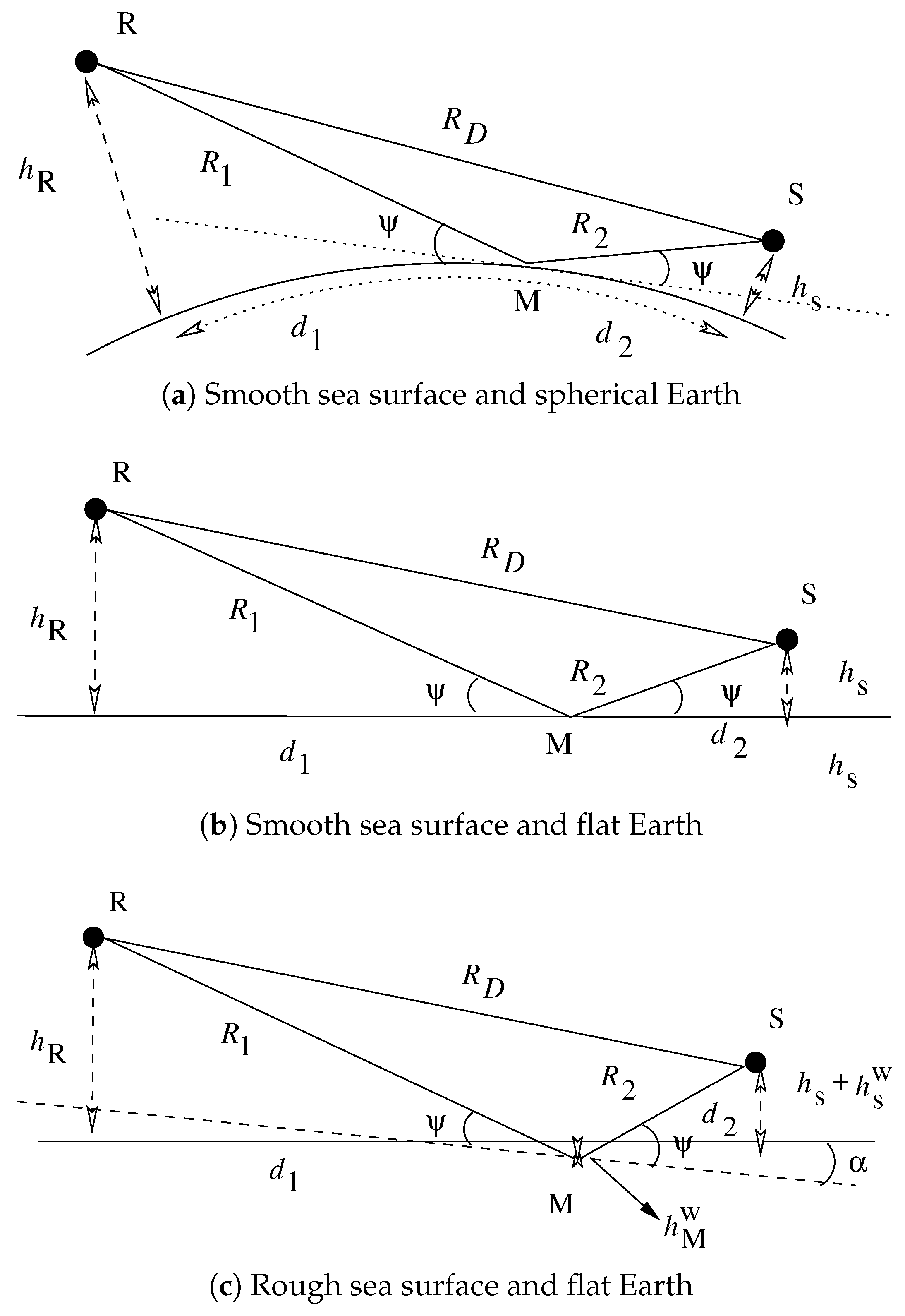
Figure 2.
Direct (red), Direct-Indirect and Indirect-Direct (blue), Indirect (green) paths and associated dimensions.
Figure 2.
Direct (red), Direct-Indirect and Indirect-Direct (blue), Indirect (green) paths and associated dimensions.
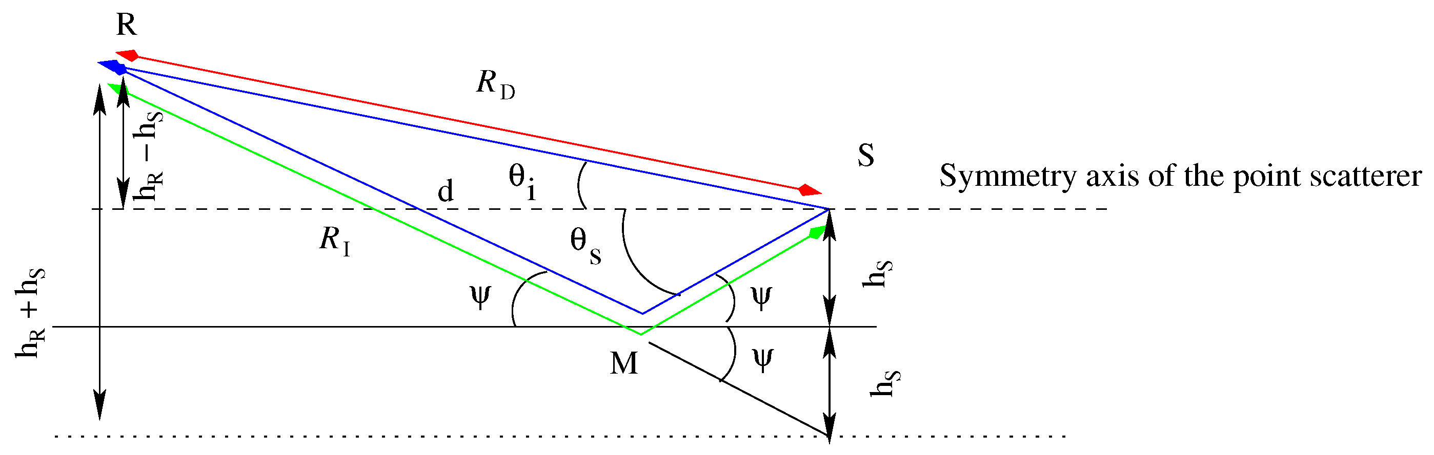
Figure 3.
and values for different grazing angles and radar frequencies.

Figure 4.
for = 0.5 m (left) and = 10 m (right).
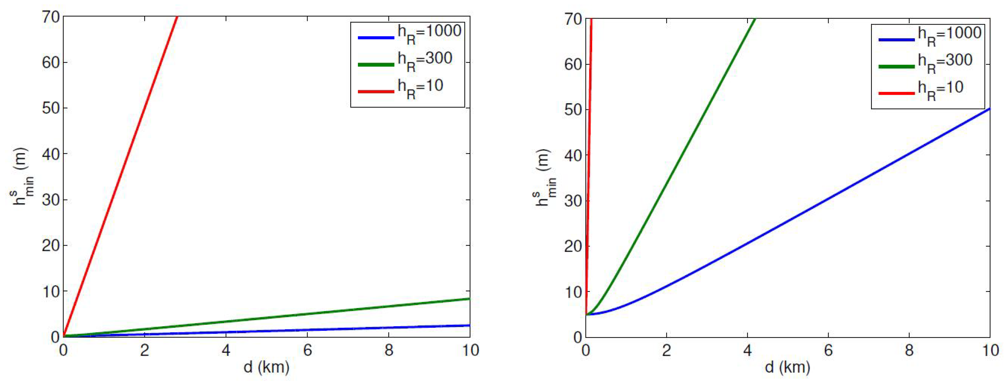
Figure 5.
Compressed range profile for = 3 m, = 1000 m, d = 10,000 m for a flat sea surface and without noise. The true scatterer location is at 0 meters in the six subfigures.
Figure 5.
Compressed range profile for = 3 m, = 1000 m, d = 10,000 m for a flat sea surface and without noise. The true scatterer location is at 0 meters in the six subfigures.

Figure 6.
Example of inverse Fourier transform of for GHz, m, m for m, HH (a) and VV (b) and m HH (c) and VV (d).
Figure 6.
Example of inverse Fourier transform of for GHz, m, m for m, HH (a) and VV (b) and m HH (c) and VV (d).

Figure 7.
Example of inverse Fourier transform of for = 0.1 GHz, m, m for m, HH (a) and VV (b) and m HH (c) and VV (d).
Figure 7.
Example of inverse Fourier transform of for = 0.1 GHz, m, m for m, HH (a) and VV (b) and m HH (c) and VV (d).

Figure 8.
Percentage of operable pulses (a), relative bias (b) and relative standard deviation (c) as a function of the central frequency , polarization and resolution .
Figure 8.
Percentage of operable pulses (a), relative bias (b) and relative standard deviation (c) as a function of the central frequency , polarization and resolution .
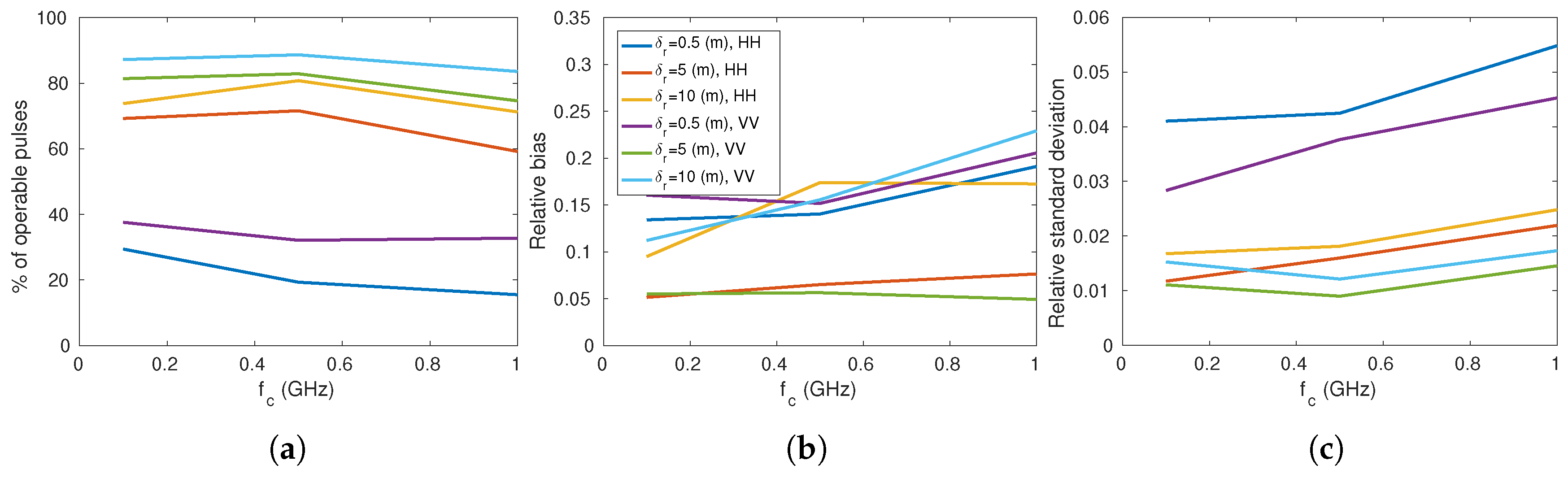
Figure 9.
Percentage of operable pulses (a), relative bias (b) and relative standard deviation (c) as a function of the sampling frequency , the radar height , the scatterer height and the projected radar distance d.
Figure 9.
Percentage of operable pulses (a), relative bias (b) and relative standard deviation (c) as a function of the sampling frequency , the radar height , the scatterer height and the projected radar distance d.
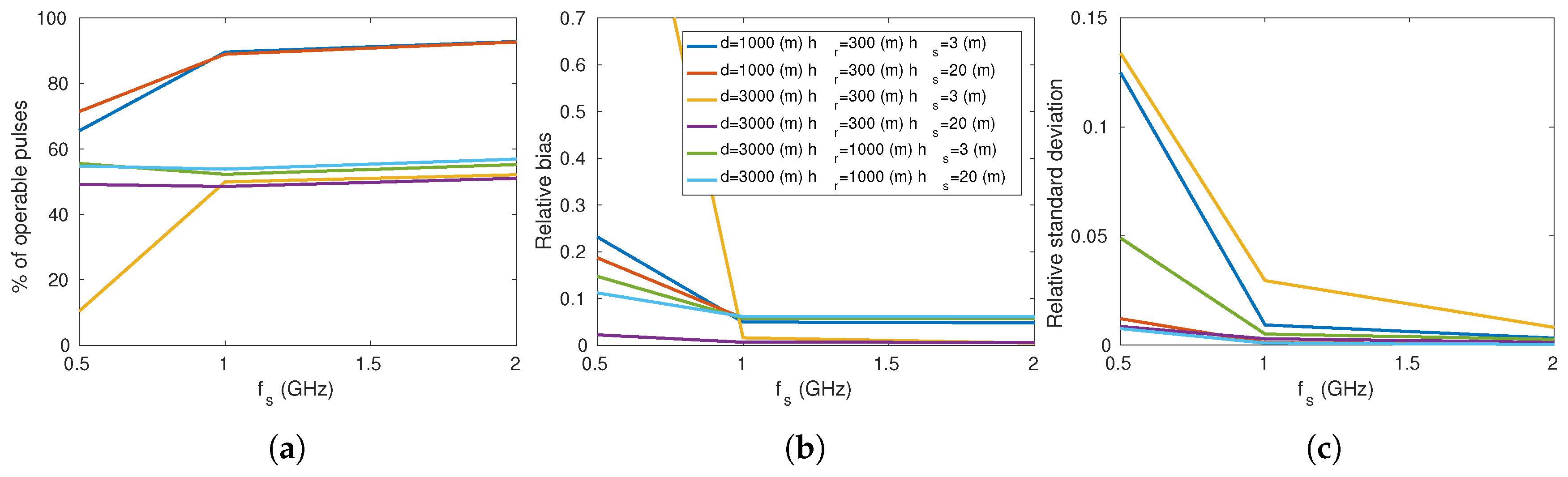
Figure 10.
Percentage of operable pulses (a), relative bias (b) and relative standard deviation (c) as a function of the projected radar distance d, the radar height , the scatterer height ( m, = 0.5 GHz, = 1 GHz).
Figure 10.
Percentage of operable pulses (a), relative bias (b) and relative standard deviation (c) as a function of the projected radar distance d, the radar height , the scatterer height ( m, = 0.5 GHz, = 1 GHz).
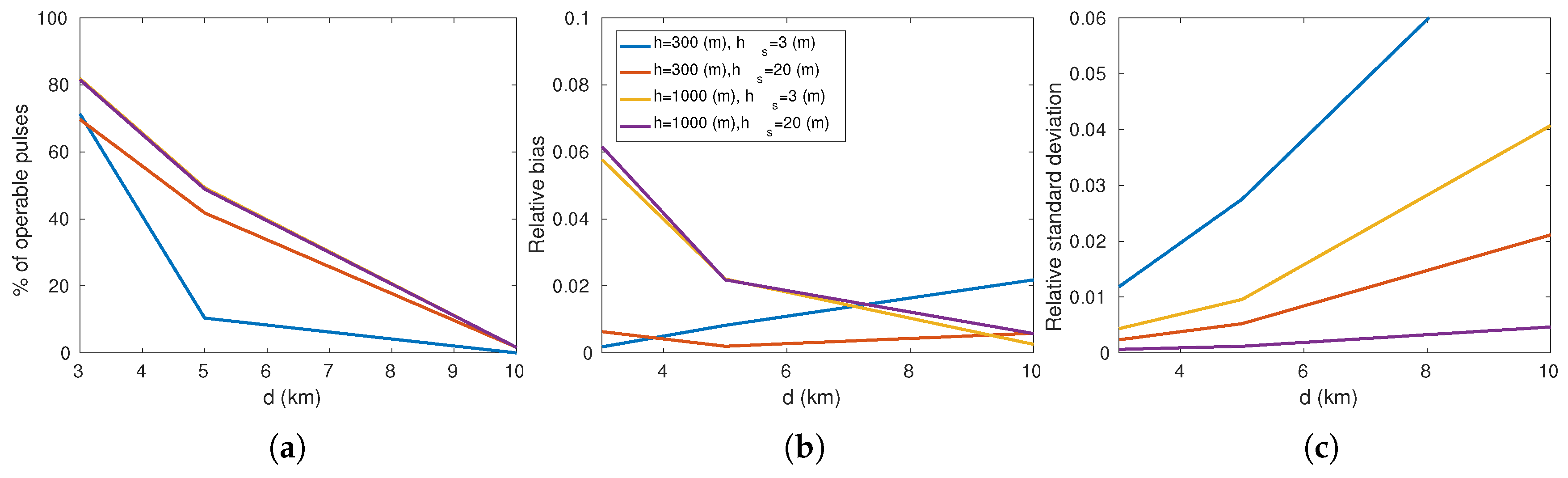
Figure 11.
Examples of Inverse Fourier transform of for two point scatterers (VV a, HH b) = 3 m and = 20 m.
Figure 11.
Examples of Inverse Fourier transform of for two point scatterers (VV a, HH b) = 3 m and = 20 m.


Table 1.
Radar/ship/sea parameters used in 2-D profile simulation.
| Notation | Name | Value |
|---|---|---|
| Central frequency | 0.1 0.5 1 (GHz) | |
| Sampling frequency | 0.5 1 2 (GHz) | |
| Radar resolution | 0.5 5 10 (m) | |
| Polarization | HH VV | |
| PRF | Pulse Repetition Frequency | 50 Hz |
| Sea surface propagation direction | 0 45 90 (degrees) | |
| Wind speed | 5 10 (m) | |
| d | Projected distance between the radar and the point scatterer | 1 3 5 10 (km) |
| Height of the radar | 10, 300, 1000 (m) | |
| Height of scatterer | 3, 20 (m) | |
| Sea surface height at the reflection point | ||
| Sea surface height at the scatterer location |
Table 2.
Parameter values for the different geometric models (for spherical earth model, , and are detailed in Appendix A), where , the Earth radius (6371 Km) and as said in Section 2.1, .
Table 2.
Parameter values for the different geometric models (for spherical earth model, , and are detailed in Appendix A), where , the Earth radius (6371 Km) and as said in Section 2.1, .
| Geometric Model | D | Reference | |
|---|---|---|---|
| Smooth sea surface and spherical earth | [47] | ||
| Smooth sea surface and flat earth | 1 | ||
| Rough sea surface and flat earth | 1 | [11] |
Table 3.
Monostatic and bistatic RCS for three kinds of scatterer: and are the incident and scattering angles (with regard to the horizontal plane), a is the sphere radius, r and H are the cylinder radius and height, b is the trihedral side length, and see [58].
Table 3.
Monostatic and bistatic RCS for three kinds of scatterer: and are the incident and scattering angles (with regard to the horizontal plane), a is the sphere radius, r and H are the cylinder radius and height, b is the trihedral side length, and see [58].
| Point Scatterer | Monostatic RCS | Bistatic RCS |
|---|---|---|
| Sphere | ||
| Cylinder | ||
| Trihedral |
Table 4.
Results for different features.
| Percentage | Relative | Relative | |
|---|---|---|---|
| of Operable Pulses | Bias | Standard Deviation | |
| HH | 66.75 | 12.2 | 1.76 |
| VV | 54.45 | 11.5 | 2.24 |
| Sphere ( m) | 54.49 | 6.97 | 1.72 |
| Sphere ( m) | 75.55 | 14.56 | 2.39 |
| Cylinder ( m, m) | 36.14 | 10.10 | 1.39 |
| Cylinder ( m, m) | 72.62 | 14.01 | 2.48 |
| Trihedral ( m) | 53.86 | 12.02 | 1.81 |
| Trihedral ( m) | 71.08 | 12.15 | 1.88 |
| m | 43.54 | 18.74 | 2.51 |
| m | 54.75 | 8.30 | 1.09 |
| m | 58.17 | 17.20 | 3.65 |
| m | 63.03 | 6.68 | 0.34 |
© 2019 by the authors. Licensee MDPI, Basel, Switzerland. This article is an open access article distributed under the terms and conditions of the Creative Commons Attribution (CC BY) license (http://creativecommons.org/licenses/by/4.0/).
Share and Cite
MDPI and ACS Style
Le Caillec, J.-M.; Habonneau, J.; Khenchaf, A. Ship Profile Imaging Using Multipath Backscattering. Remote Sens. 2019, 11, 748. https://doi.org/10.3390/rs11070748
AMA Style
Le Caillec J-M, Habonneau J, Khenchaf A. Ship Profile Imaging Using Multipath Backscattering. Remote Sensing. 2019; 11(7):748. https://doi.org/10.3390/rs11070748
Chicago/Turabian StyleLe Caillec, Jean-Marc, Jérôme Habonneau, and Ali Khenchaf. 2019. "Ship Profile Imaging Using Multipath Backscattering" Remote Sensing 11, no. 7: 748. https://doi.org/10.3390/rs11070748
Note that from the first issue of 2016, this journal uses article numbers instead of page numbers. See further details here.